Lattice study on scattering with moving wall source
Abstract
The -wave pion-kaon () scattering lengths at zero momentum are calculated in lattice QCD with sufficiently light quarks and strange quark at its physical value by the finite size formula. The light quark masses correspond to GeV. In the “Asqtad” improved staggered fermion formulation, we measure the four-point correlators for both isospin and channels, and analyze the lattice simulation data at the next-to-leading order in the continuum three-flavor chiral perturbation theory, which enables us a simultaneous extrapolation of scattering lengths at physical point. We adopt a technique with the moving wall sources without gauge fixing to obtain the substantiable accuracy, moreover, for channel, we employ the variational method to isolate the contamination from the excited states. Extrapolating to the physical point yields the scattering lengths as and for and channels, respectively. Our simulation results for scattering lengths are in agreement with the experimental reports and theoretical predictions, and can be comparable with other lattice simulations. These simulations are carried out with MILC flavor gauge configurations at lattice spacing fm.
pacs:
12.38.GcI Introduction
Pion-kaon () scattering at low energies is the simplest reactions including a strange quark, and it allows for an explicit exploration of the three-flavor structure of the low-energy hadronic interactions, which is not directly probed in the scattering. The measurement of scattering lengths is one of the cleanest processes and a decisive test for our understanding of the chiral symmetry breaking of the quantum chromodynamics (QCD). In the present study, we will concentrate on the -wave scattering lengths of system, which have two isospin eigenchannels () in the isospin limit, and the low-energy interaction is repulsive for channel, and attractive for case, respectively.
Experimentally, scattering lengths are obtained through scattering phases using the Roy-Stainer equations. The experiments at low energies are an important method in the study of the interactions among mesons matison74:Kpi_exp_a ; johannesson73:Kpi_exp_b ; shaw80:Kpi_exp_c , and these experiments have reported that the -wave scattering length () in the channel, has a small negative value, namely, . Moreover, the on-going experiments proposed by the DIRAC collaboration dirac to examine atoms will provide the direct measurements or constraints on scattering lengths.
At present, theory predicts scattering lengths with a precision of about , and it will be significantly improved in the near future. Through the scalar form factors in semi-leptonic pseudo-scalar-to-pseudo-scalar decays, Flynn et al. Fly07 extracted the scattering length in the channel as = +0.179(17)(14). Three-flavor Chiral Perturbation Theory (PT) Bernard:1990kw ; Ber91b ; Kubis:2001bx ; Bue03 has been used to predict the scattering lengths in the study of the low-energy scattering, and small negative value was claimed as . However, if the scattering hadrons contain strange quarks, PT predictions usually suffer from considerable corrections due to the chiral flavor symmetry breaking, as compared with the case of the scattering. Therefore, a lattice QCD calculation is needed to offer an alternative important consistent check of the validity of PT in the presence of the strange quarks.
To date, four lattice studies of scattering length have been reported Miao:2004gy ; Beane:2006gj ; Nagata:2008wk ; Sasaki:2010zz . The first lattice calculation of scattering length in channel was explored by Miao et al. Miao:2004gy using the quenched approximation, and the value of was found to be . The first fully-dynamical calculation using flavors of the Asqtad-improved Orginos:1998ue ; Orginos:1999cr staggered sea quark Bernard:2010fr ; Bazavov:2009bb was carried out Beane:2006gj to calculate the scattering length for GeV, and further indirectly evaluate the scattering length on the basis of PT. They obtained a small negative value of for channel and a positive value of for channel, respectively. Nagata et al. fulfilled first direct lattice calculation on channel Nagata:2008wk using the quenched approximation. They investigated all quark diagrams contributing to both isospin eigenstates, and found that the scattering amplitudes can be expressed as the combinations of only three diagrams in the isospin limit. This work greatly inspires us to study scattering. However, they did not observe the repulsive interaction even for channel at their simulation points, and their lattice calculations are relatively cheaper. Sasaki et al. observed the correct repulsive interaction for channel and attractive for case, and they obtained the scattering lengths of and for the and channels, respectively Sasaki:2010zz . Moreover, to isolate the contamination from the excited states, they construct a matrix of the time correlation function and diagonalize it Sasaki:2010zz , this method will guide us to study scattering for channel in a correct manner. It should be stressed that, to reduce the computational cost, they employed a technique with a fixed kaon sink operator for the calculation of scattering length for channel and then an exponential factor is introduced to drop the unnecessary -dependence appearing due to the fixed kaon sink time Sasaki:2010zz . In this work, we will improve this technique by using a “moving” wall source without gauge fixing where the exponential factor is not needed any more. Thus, there is no satisfactory direct lattice calculation for channel until now.
In the present study, we will use the MILC gauge configurations generated in the presence of flavors of the Asqtad improved Orginos:1998ue ; Orginos:1999cr staggered dynamical sea quarks Bernard:2010fr ; Bazavov:2009bb to study the -wave scattering lengths for both and channels. Inspired by the exploratory study of scattering for channel in Ref. Kuramashi:1993ka , we will adopt almost same technique but with moving kaon wall source operator without gauge fixing for and channels to obtain the reliable accuracy. We calculated all the three diagrams categorized in Ref. Nagata:2008wk , and observed a clear signal of attraction for channel and that of repulsion for case. Moreover, for channel, we employ the variational method to isolate the contamination from the excited states. Most of all, we only used the lattice simulation data of our measured scattering lengths for both isospin eigenstates to simultaneously extrapolate toward the physical point using the continuum three-flavor PT at the next-to-leading order. Our lattice simulation results of the scattering lengths for both isospin eigenchannels are in accordance with the experimental reports and theoretical predictions, and can be comparable with other lattice simulations.
This article is organized as follows. In Sec. II we describe the formalism for the calculation of scattering lengths including the Lüscher’s formula Luscher:1991p2480 ; Luscher:1990ck ; Lellouch:2001p4241 and our computational technique of the modified wall sources for the measurement of four-point functions. In Sec. III we will show the simulation parameters and our concrete lattice calculations. We will present our lattice simulation results in Sec. IV, and arrive at our conclusions and outlooks in Sec. V.
II Method of measurement
In this section, we will briefly review the formulas of the -wave scattering length from two-particle energy in a finite box, with emphasis on the formulae for isospin system. Also we will present the detailed procedure for extracting the the energies of system. Here we follow the original derivations and notations in Refs. Nagata:2008wk ; Sharpe:1992pp ; Kuramashi:1993ka ; Fukugita:1994na ; Fukugita:1994ve .
II.1 four-point functions
Let us consider the scattering of one Nambu-Goldstone pion and one Nambu-Goldstone kaon in the Asqtad-improved staggered dynamical fermion formalism. Using operators for pions at points , and operators for kaons at points , respectively, with the pion and kaon interpolating field operators defined by
| (1) | |||||
| (2) | |||||
| (3) | |||||
| (4) |
we then represent the four-point functions as
| (5) |
where represents the expectation value of the path integral, which we evaluate using the lattice QCD simulations.
After summing over spatial coordinates , , and , we obtain the four-point function in the zero-momentum state,
| (6) |
where , , , and , and stands for the time difference, namely, .
To avoid the complicated Fierz rearrangement of the quark lines, we choose the creation operators at the time slices which are different by one lattice time spacing as is suggested in Ref. Fukugita:1994ve , namely, we select , and . In system, there are two isospin eigenstates, namely, and , we construct the operators for these isospin eigenchannels as Nagata:2008wk
| (7) | |||||
| (8) |
where
| (9) | |||||
| (10) |
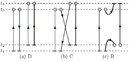
If we assume that the and quarks have the same mass, only three diagrams contribute to scattering amplitudes Nagata:2008wk . The quark line diagrams contributing to four-point function denoted in Eq. (6) are displayed in Figure 1, labeling them as direct (D), crossed (C) and rectangular (R), respectively. The direct and crossed diagrams can be easily evaluated by constructing the corresponding four-point amplitudes for arbitrary values of the time slices and using only two wall sources placed at the fixed time slices and . However, the rectangular diagram (R) requires another quark propagator connecting the time slices and , which make the reliable evaluation of this diagram extremely difficult.
Sasaki et al. solve this problem through the technique with a fixed kaon sink operator to reduce the computational cost Sasaki:2010zz . Encouraged by the exploratory works of the scattering at channel in Refs. Kuramashi:1993ka ; Fukugita:1994ve , similarly, we handle this problem by evaluating quark propagators on a lattice, each propagator, which corresponds to a wall source at the time slice , is denoted by
| (11) |
where is the quark matrix for the staggered Kogut-Susskind quark action. The combination of which we apply for four-point functions is schematically shown in Figure 1, where short bars stand for the position of wall source, open circles are sinks for local pion or kaon operators, and the thinker lines represent the strange quark lines. Likely, the subscript in the quark propagator represents the position of the wall source. , , and , are schematically displayed in Figure 1, and we can also expressed them in terms of the quark propagators , namely,
| (12) | |||||
| (13) | |||||
| (14) |
where daggers mean the conjugation by the even-odd parity for the staggered Kogut-Susskind quark action, and stands for the trace over the color index. The hermiticity properties of the propagator are used to eliminate the factors of .
For rectangular diagram in Figure 1(c), it creates the gauge-variant noise Kuramashi:1993ka ; Fukugita:1994ve . One can reduce the noise by fixing gauge configurations to some gauge ( e.g., Coulomb gauge), and select a special wall source to emit only the Nambu-Goldstone pion Gupta:1990mr , however, the gauge non-invariant states may contaminate the four-point function. Alternatively, we perform the gauge field average without gauge fixing since the gauge dependent fluctuations should neatly cancel out among the lattice configurations. Besides these cancelations, the summation of the gauge-variant terms over the spatial sites of the wall source further suppresses the gauge-variant noise. In our current lattice simulation we found that this method works pretty well.
All three diagrams in Figure 1 are needed to be calculated to study the scattering in both and channels. Three types of the propagators can be combined to construct the physical correlation functions for states with definite isospin. As it is investigated in Ref. Nagata:2008wk , in the isospin limit, the correlation function for and channels can be expressed as the combinations of three diagrams, namely,
| (15) | |||||
| (16) |
where the operator denoted in Eq. (7) creates a state with total isospin and the staggered-flavor factor is inserted to correct for the flavor degrees of freedom of the Kogut-Susskind staggered fermion Sharpe:1992pp . For the pion and kaon operators it is most natural to choose the one in the Nambu-Goldstone channel. This is the choice for our current study.
To calculate the scattering lengths for hadron-hadron scattering on the lattice, or the scattering phase shifts in general, one usually resorts to Lüscher’s formula which relates the exact energy level of two hadron states in a finite box to the scattering phase shift in the continuum. In the case of scattering, the -wave scattering length in the continuum is defined by
| (17) |
is the magnitude of the center-of-mass scattering momentum which is related to the total energy of the system with isospin in a finite box of size by
| (18) |
where the is the pion mass, and is the kaon mass. We can rewrite Eq. (18) to an elegant form as
| (19) |
In the absence of the interactions between the and particles, , and the energy levels occur at momenta , ( is a integer), corresponding to the single-particle modes in a cubic box. is the -wave scattering phase shift, which can be evaluated by the Lüscher’s finite size formula Luscher:1991p2480 ; Lellouch:2001p4241 ,
| (20) |
where the zeta function is denoted by
| (21) |
here is no longer an integer, and can be efficiently calculated by the method described in Ref. Yamazaki:2004qb . We also discussed this technique in Appendix A, where we extend this discussion to the case with the negative . In the case of the attractive interaction, on the bound state has a negative value, therefore is pure imaginary, and is no longer physical scattering phase shift Sasaki:2010zz . , however, still have a real value even for this case, hence obtained by Eq. (20) is also real. If is enough small, we can consider as the physical scattering length at threshold Sasaki:2010zz .
The energy of system with isospin can be obtained from four-point function denoted in Eq. (15) with the large . At large these correlators will behave as Mihaly:1997 ; Mihaly:Ph.D
| (23) | |||||
where is the energy of the lightest state with isospin . The terms alternating in sign are a peculiarity of the Kogut-Susskind formulation of the lattice fermions and correspond to the contributions from intermediate states with opposite parity Mihaly:1997 ; Mihaly:Ph.D . The ellipsis suggests the contributions from excited states which are suppressed exponentially.
We should bear in mind that, for the staggered Kogut-Susskind quark action, there are further complications in itself stemming from the non-degeneracy of pions and kaons in the Goldstone and other channels at a finite lattice spacing. Briefly speaking, the contributions of non-Nambu-Goldstone pions and kaons in the intermediate states is exponentially suppressed for large times due to their heavier masses compared to these of the Nambu-Goldstone pion and kaon Sharpe:1992pp ; Kuramashi:1993ka ; Fukugita:1994ve . Thus, we suppose that interpolator does not couple significantly to other tastes, and neglect this systematic errors.
In our concrete calculation, we calculated the pion mass and kaon mass through the methods discussed by the MILC collaboration in Refs. Bernard:2001av ; Aubin:2004wf in our previous study fzw:2011cpc12 . In this work we evaluate total energy of system with isospin from Eq. (23).
In the current study we also evaluate the energy shift from the ratios
| (24) |
where and are the pion and kaon two-point functions, respectively. Considering Eq. (15), we can write the amplitudes which project out the and isospin eigenstates as
| (25) | |||||
| (26) |
Following the discussions in Ref. Sharpe:1992pp , we now then can extract the energy shift from the ratios
| (27) |
where stands for wave function factor, which is the ratio of two amplitudes from the four-point function and the square of the pion two-point correlator and the kaon two-point correlator, and the ellipsis indicates the terms suppressed exponentially. In , some of the fluctuations which contribute to both the two-point and four-point correlation functions neatly cancel out, hence, improving the quality of the extraction of the energy shift as compared with what we can obtain from an analysis through the individual correlation functions Beane:2006gj .
For channel, we can use Eq. (23) or Eq. (27) to extract the energy shifts . We have numerically compared the fitting values from two methods, and found well agreement within statistical errors. In fact, using Eq. (27) to extract the energy shift has been extensively employed for the study of scattering at case in Ref. Beane:2006gj . Hence, in this work, we will only present the energy shifts calculated by Eq. (27), and then its corresponding scattering lengths.
On the other hand, for channel, the presence of the kappa resonance is clearly shown in the low energy Sasaki:2010zz , and therefore it should be necessary for us to separate the ground state contribution from the contamination stemming from the excited states to achieve the reliable scattering length as it is investigated in Ref. Sasaki:2010zz . For this purpose, we will construct a correlation matrix of the time correlation function and diagonalize it to extract the energy of the ground state.
II.2 Correlation matrix
For channel, to separate the contamination from the excited states, we construct a matrix of the time correlation function,
| (28) |
where is an interpolating operator for the meson with zero momentum, and is an interpolating operator for system which is extensively discussed in section II.1. The interpolating operator employed here is exactly the same as these in our previous studies in Refs. fzw:2011cpc12 ; Fu:2011xb ; Fu:2011xw , the notations adopted here are also the same, but to make this paper self-contained, all the necessary definitions will be also presented below.
II.2.1 sector
In our previous studies fzw:2011cpc12 ; Fu:2011xb ; Fu:2011xw , we have presented a detailed procedure to measure kappa correlator . To simulate the correct number of quark species, we use the fourth-root trick Aubin:2003mg , which automatically performs the transition from four tastes to one taste per flavor for staggered fermion at all orders. We employ an interpolation operator with isospin and at the source and sink,
| (29) |
where is the indices of the taste replica, is the number of the taste replicas, is the color indices, and we omit the Dirac-Spinor index. The time slice correlator for the meson in the zero momentum state can be evaluated by
where are the spatial points of the state at source and sink, respectively. After performing Wick contractions of fermion fields, and summing over the taste index, for the light quark Dirac operator and the quark Dirac operator , we obtain fzw:2011cpc12
| (30) |
where Tr is the trace over the color index, and is the lattice position.
For the staggered quarks, the meson propagators have the generic single-particle form,
| (31) |
where the oscillating terms correspond to a particle with opposite parity. For meson correlator, we consider only one mass with each parity in Eq. (31), namely, in our concrete calculation, our operator is the state with spin-taste assignment and its oscillating term with fzw:2011cpc12 . Thus, the correlator was fit to the following physical model,
| (32) |
where and are two overlap factors. In Figure 6, we clearly note this oscillating term.
We should bear in mind that, for the staggered Kogut-Susskind quark action, our interpolating operator couples to various tastes as we examined the scalar and mesons in Refs. Bernard:2007qf ; Bernard:2006gj , where we investigated two-pseudoscalar intermediates states (namely, bubble contribution). In Ref. Fu:2011xb , we investigated the extracted masses with and without bubble contribution for kappa correlators. We found that there are only about differences in masses, although the bubble contributions are dominant in the correlators at large time region. Thus, in the current study, we can reasonably assume that the interpolator does not couple remarkably to other tastes, and ignore this systematic errors for the sector Fu:2011xw .
II.2.2 Off-diagonal sector
The calculations of the off-diagonal elements in correlation matrix in Eq. (28), namely, and are exactly the same as these in our previous study for non-zero momenta in Ref. Fu:2011xw , the notations adopted here are also the same, but to make this paper self-contained, all the necessary definitions will be also presented below.
To avoid the complicated Fierz rearrangement of the quark lines, we choose the creation operators at the time slices which are different by one lattice time spacing as suggested in Ref. Fukugita:1994ve , namely, we select , and for three-point function, and choose , and for three-point function.

The quark line diagrams contributing to the and three-point function are plotted in Figure 2(a) and Figure 2(b), respectively, where short bars stand for the position of wall source, open circles are sinks for local pion or kaon operators, and the thinker lines represent the strange quark lines. Likely, the subscript in the quark propagator represents the position of the wall source.
The three-point function can be easily evaluated by constructing the corresponding three-point amplitudes for arbitrary values of the time slice using only two wall sources placed at the fixed time slices and . However, the calculation of three-point function is almost the same difficult as that of the rectangular diagram for four-point correlator function, since it requires another quark propagator connecting time slices and . The and three-point functions are schematically shown in Figure 2, and we can also express them in terms of the quark propagators , namely,
| (33) | |||||
| (34) |
II.3 Extraction of energies
Through calculating the matrix of correlation function denoted in Eq. (28), we can separate the ground state from first excited state in a clean way. It is very important to map out “avoided level crossings” between the resonance and its decay products (namely, and ) in a finite box volume, because the first excited state is potentially close to the ground state. This makes the extraction of the ground state energy unfeasible if we only utilize a single exponential fit ansatz. Since we can not predict a priori whether our energy eigenvalues are near to the resonance region or not, we find it always safe in practice to adopt the correlation matrix to analyze our lattice simulation data for isospin channel. To extract the ground state, we follow the variational method Luscher:1990ck and construct a ratio of correlation function matrices as
| (35) |
with some reference time slice Luscher:1990ck , which is assumed to be large enough such that the contributions to correlation matrix from the excited states can be neglected, and the lowest two eigenstates dominate the correlation function. The two lowest energy levels can be extracted by a proper fit to two eigenvalues () of matrix . Because here we work on the staggered fermions, and we can easily prove that () behaves as Fu:2011xw
| (37) | |||||
for a large , which mean to suppress the excited states and the unwanted thermal contributions. This equation explicitly contains an oscillating term. For the current study, we are only interested in eigenvalue , here non-degenerate eigenvalues are assumed. In practice, we found that the oscillating term in is not appreciable for some , we can also adopt following simple fitting model Fu:2011xw ,
| (38) |
and the difference between the fitting models of Eq. (37) and Eq. (38) is small. However, to make our extracted ground energy for isospin channel always reliable, in this work, we will present the ground energy calculated by Eq. (37), and then its corresponding -wave scattering lengths.
III Lattice calculation
III.1 Simulation parameters
We used the MILC lattices with dynamical flavors of the Asqtad-improved staggered dynamical fermions, the detailed description of the simulation parameters can be found in Refs. Bernard:2010fr ; Bazavov:2009bb . One thing we must stress that the MILC configurations are generated using the staggered formulation of lattice fermions Kaplan:1992bt ; Shamir:1993zy ; Shamir:1998ww with rooted staggered sea quarks Bernard:2001av which are hypercubic-smeared (HYP-smeared) Hasenfratz:2001hp ; DeGrand:2002vu ; DeGrand:2003in ; Durr:2004as . As it was shown in Refs. Renner:2004ck ; Edwards:2005kw that HYP-smearing gauge links significantly improves the chiral symmetry.
We analyzed four-point functions on the fm MILC lattice ensemble of gauge configurations with bare quark masses and and bare gauge coupling , which has a physical volume approximately fm. The inverse lattice spacing GeV Bernard:2010fr ; Bazavov:2009bb . The mass of the dynamical strange quark is near to its physical value, and the masses of the and quarks are degenerate. To avoid the contamination from pions and kaons propagating backward in time, periodic boundary condition is applied to the three spatial directions while in the temporal direction, Dirichlet boundary condition is imposed, which reduce the original time extent of down to , moreover, it avoids the “fake effects” discussed in Ref. Sasaki:2010zz .
III.2 Sources for isospin channel
To calculate the correlation functions, we use the standard conjugate gradient method (CG) to obtain the required matrix element of the inverse fermion matrix. The calculation of the correlation function for the rectangular diagrams naturally requires us to compute the propagators on all the time slices of both source and sink, which requires the calculation of separate propagators in our lattice simulations. After averaging the correlator over all possible values, the statistics are greatly improved since we can put the pion source and kaon source at all possible time slices, namely, the correlator is calculated through
| (39) | |||||
| (40) |
The best-effort to generate the propagators on all time slices enables us to obtain the correlators with high precision, which is vital to extract the desired scattering phase shifts reliably.
For each time slice, six fermion matrix inversions are required corresponding to the possible color choices for the pion source and kaon source, respectively, and each inversion takes about one thousand iterations during the CG calculation. Therefore, all together we carry out inversions on a full QCD configuration. As shown follow, this large number of inversions, performed on configurations, provides the substantial statistics needed to resolve the real parts of the and amplitudes with reliable accuracy.
In the calculation of the off-diagonal correlator, , the quark line contractions results in a three-point diagram. Since in this three-point diagram the pion field and kaon field are located at the source time slice , , respectively. We calculate the off-diagonal correlator through
| (41) | |||||
| (42) |
where, again, we sum the correlator over all time slices and average it. As for the second off-diagonal correlator , the pion field and kaon field are placed at the sink time slices and , respectively, which make the computation of difficult. However, using the relation , we can obtain the matrix element for free. As it is studied in Ref. Aoki:2007rd , since the sink and source operators are identical for a large number of configurations, is a Hermitian matrix. The component agrees with within the error, but the statistical errors of the matrix element should be larger than that of matrix element for a large . Therefore, in the following analyses we substitute matrix element by the complex conjugate of matrix element , which is not only to save about computation time, but also significantly to reduce statistical errors.
For the correlator, , we have measured the point-to-point correlators with high precision in our previous work fzw:2011cpc12 . Therefore, we can exploit the available propagators to construct the -correlator
| (43) |
where, also, we sum the correlator over all time slices and average it.
One thing we must stress that, in the calculation of the correlator , we make our best-efforts to reliably measure the rectangular diagram, since the other two diagrams are relatively easy to evaluate. We found that the rectangular diagram plays a major role in this correlator. Therefore, we get it properly for the sector for isospin channel.
In this work, we also measure two-point correlators for pion and kaon, namely,
| (44) | |||||
| (45) |
where the is correlation function for the pion with zero momentum, and the is correlation function for the kaon with zero momentum.
IV Simulation results
In our previous work fzw:2011cpl , we have measured the pion and kaon point-to-point correlators. Using these correlators, we can precisely extract the pion mass () and kaon mass () fzw:2011cpl , which are summarized in Table 1. Using the same method discussed in Ref. Aubin:2004fs and the MILC code for calculating the pion decay constants , we precisely extract the pion decay constants Fu:2011bz , which are in agreement with the previous MILC determinations at this same lattice ensemble in Ref. Bazavov:2009bb . Here we used all the lattice configurations of this ensemble. We also recapitulated these fitted values in Table 1.
IV.1 Diagrams , and
The four-point functions are calculated with same lattice configurations using six valence quarks, namely, , , , , and , where is the light valence quark mass. They all have the same strange sea quark mass , which is fixed at its physical value Bazavov:2009bb .
In Figure 3 the individual ratios, which are defined in Eq. (24) corresponding to the diagrams in Figure 1, ( and ) are displayed as the functions of for . We can note that diagram makes the biggest contribution, then diagram , and diagram makes the smallest contribution. The calculation of the amplitudes for the rectangular diagram stands for our principal work. Clear signals observed up to for the rectangular amplitude demonstrate that the method of the moving wall source without gauge fixing used here is practically applicable.
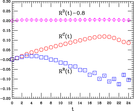
The values of the direct amplitude are quite close to unity, indicating that the interaction in this channel is very weak. The crossed amplitude, on the other hand, increases linearly, which implies a repulsion in channel. After an initial increase up to , the rectangular amplitude exhibits a roughly linear decrease up to , which suggests an attractive force between the pion and kaon in channel. Furthermore, the magnitude of the slope is similar to that of the crossed amplitude but with opposite sign. These features are what we eagerly expected from the theoretical predictions Bernard:1990kw ; Sharpe:1992pp . We can observe that the crossed and rectangular amplitudes have the same value at , and the close values for small . Because our analytical expressions in Eq. (12) for the two amplitudes coincide at , they should behave similarly until the asymptotic state is reached.
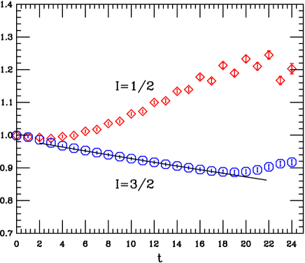
In Figure 4, we display the ratio projected onto the isospin and channels for , which are denoted in Eq. (25). A decrease of the ratio of indicates a positive energy shift and hence a repulsive interaction for channel, while an increase of suggests a negative energy shift and hence an attraction for channel. A dip at for channel can be clearly observed Fukugita:1994ve . The systematically oscillating behavior for channel in the large time region is also clearly observed, which is a typical characteristic of the Kogut-Susskind formulation of lattice fermions and corresponds to the contributions from the intermediate states of the opposite parity Mihaly:1997 ; Mihaly:Ph.D , this also clearly indicates the existence of the contaminations from other states rather than the pion-kaon scattering state Sasaki:2010zz . Therefore, to isolate the potential contaminations, we will use the variational method Luscher:1990ck to analyze the lattice simulation data. As for channel, this oscillating characteristic is not appreciable, we will use the traditional method, namely, using Eq. (27) to compute the energy shift and then calculate the corresponding scattering length.
IV.2 Fitting analyses for channel
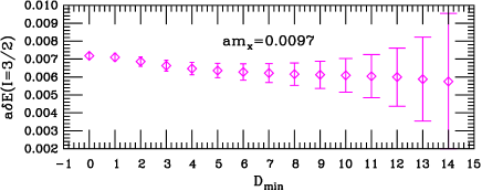

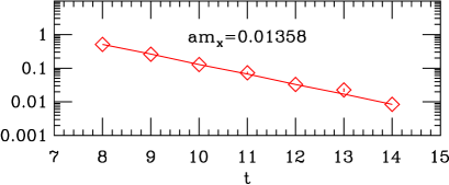
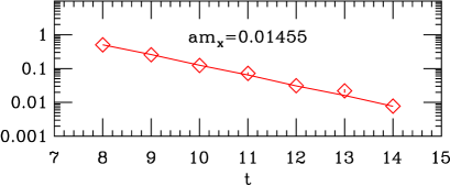
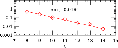
According to our discussions in Section II, in this work, we will make use of Eq. (27) to extract the energy shift for channel. Then we insert these energy shifts into the Eqs. (17) and (20) to obtain the corresponding -wave scattering lengths. Therefore, properly extracting the energy shifts is a crucial step to our final results in this paper. A convincing way to analyze our lattice simulation data is with the “effective energy shift” plots, a variant of the effective mass plots, where the propagators were fit with varying minimum fitting distances , and with the maximum distance either at the midpoint of the lattice or where the fractional statistical errors exceeded about for two successive time slices. For each valence quark , the effective energy shift plots as a function of minimum fitting distance for channel are shown in Figure 5. The central value and uncertainty of each parameter was determined by the jackknife procedure over the ensemble of gauge configurations.
The energy shifts of system for channel are extracted from the “effective energy shift” plots, and the energy shifts were selected by looking for a combination of a “plateau” in the energy as a function of the minimum distance , and a good confidence level (namely, ) for the fit. We found that the effective energy shifts for channel have only relative small errors within broad minimum time distance region and are taken to be quite reliable.
We utilize the exponential physical fitting model in Eq. (27) to extract the desired energy shifts for channel. In Figure 4 we display the ratio projected onto the and channels for , where we can watch the fitted functional form as compared with the lattice simulation data for channel. For the other five light valence quarks, we obtain the similar results, therefore we do not show these ratio plots here. The fitted values of the energy shifts, in lattice units and wave function factor for channel are summarized in Table 2. The wave function factors are pretty close to unity and the is quite small for channel, indicating the values of the extracted scattering lengths are substantially reliable.
| Isospin | Range | ||||
|---|---|---|---|---|---|
Now we can insert these energy shifts in Table 2 into the Eqs. (17) and (20) to obtain the corresponding -wave scattering lengths. The center-of-mass scattering momentum in GeV calculated by Eq. (19), from which we can easily estimate its statistcal errors. Once we obtain the values of , the -wave scattering lengths in lattice units can be obtained through Eqs. (17) and (20). All of these values are summarized in Table 3. Here we utilize pion masses and kaon masses given in Table 1. The errors of the center-of-mass scattering momentum and the -wave scattering lengths come from the statistical errors of the energy shifts energies , pion mass and kaon mass .
| Isospin | [] | |||
|---|---|---|---|---|
IV.3 Fitting analyses for channel
In Figure 6, we show the real parts of the diagonal components ( and ) and the real part of the off-diagonal component of the correlation function denoted in Eq. (28). Since is a Hermitian matrix, we will substitute the off-diagonal component by to reduce statistical errors in the following analyses.
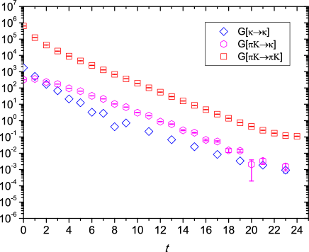
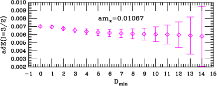
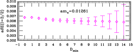
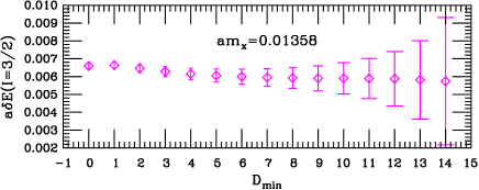
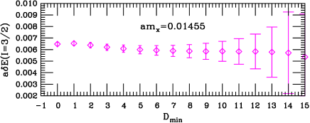
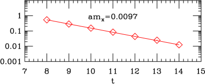
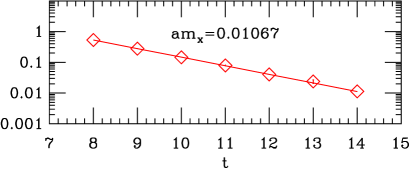
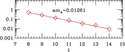
We calculate two eigenvalues () for the matrix in Eq. (35) with the reference time . In this work, we are only interested in the eigenvalue 111 In our previous study Fu:2011xw , we have preliminarily examined the behavior of . . In Figure 7 we plot our lattice results for for each valence quark in a logarithmic scale as the functions of together with a correlated fit to the asymptotic form given in Eq. (37). From these fits we then extract the energies that will be used to determine the -wave scattering lengths.
To extract the energies reliably, we must take two major sources of the systematic errors into consideration. One arises from the excited states which affect the correlator in low time slice region. The other one stems from the thermal contributions which distort the correlator in high time slice region. By denoting a fitting range and varying the values of the and , we can control these systematic errors. In our concrete fitting, we take to be and increase the reference time slice to suppress the excited state contaminations. Moreover, we select to be sufficiently far away from the time slice to avoid the unwanted thermal contributions. The fitting parameters , and are tabulated in Table 4. The corresponding fitting results in the reasonable values of . The together with the fit results for the energies for the ground state are also listed in Table 4.
| Isospin | ||||||
|---|---|---|---|---|---|---|
Now we can insert these energies in Table 4 into the Eqs. (17) and (20) to obtain the scattering lengths. The center-of-mass scattering momentum in GeV calculated by Eq. (19) and thence the corresponding -wave scattering lengths in lattice units obtained through Eqs. (17) and (20) are summarized in Table 5. Here we use the pion masses and kaon masses given in Table 1. The errors of the center-of-mass scattering momentum and the -wave scattering lengths are calculated from the statistic errors of the energy shifts energies , pion mass and kaon mass .
| Isospin | [] | |||
|---|---|---|---|---|
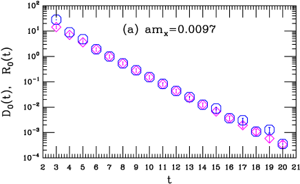
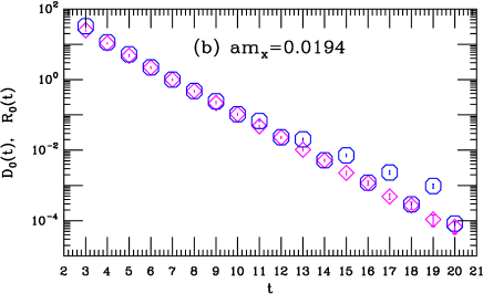
To examine the effects of the contaminations from the excited states for channel, we denote the ratios of and which is the lowest eigenvalue of , to the correlator Sasaki:2010zz ,
| (46) | |||||
| (47) |
In the upper panel of Figure 8, we show (magenta diamonds) and (blue octagons) at GeV. We can note that the difference of two ratios is small. This suggests that the contamination from the excited states is negligible at this light quark mass. However, from the bottom panel of Figure 8, we observe that the contamination from the excited states is not negligible at GeV, and the diagonalization obviously changes the characteristics of the ratio, since the interpolative operator for channel has a large overlap with the excited states Sasaki:2010zz . Therefore, we further confirmed that the separation of the contamination from the excited states is absolutely necessary for the heavy quark masses Sasaki:2010zz when we study the scattering for channel.
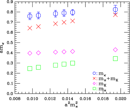
Using the fitting models discussed in Ref. Aubin:2004wf , we extract the pion and kaon masses fzw:2011cpl . And using the fitting model in Eq (32), we calculate the kappa mass Fu:2011xb . In Figure 9, we display , and threshold in lattice units as the functions of the pion mass . We observe that, as the valence quark mass increases, threshold grows faster than mass and, as a consequence, for the heavy quark masses, threshold is close to the mass. In Figure 9, we can clearly note that threshold is very close to the mass for light quark mass . This can be in part explained why the separation of the contamination from the excited states is indispensable for the large quark masses Sasaki:2010zz .
IV.4 Chiral extrapolations and scattering length
In the present study, we employ a reasonable small pion masses , namely, GeV, which are still considerably larger than its physical ones, therefore, we need to extrapolate the -wave scattering lengths toward the physical point. For this purpose, we employ the formula predicted by chiral perturbation theory to next-to-leading order (NLO) Bernard:1990kw ; Kubis:2001bx ; Beane:2006gj ; Sasaki:2010zz ; Chen:2006wf . In chiral perturbation theory at NLO, we provide the continuum PT forms of and , which can be directly constructed from Refs. Kubis:2001bx ; Beane:2006gj ; Sasaki:2010zz ,
| (48) | |||||
| (49) |
where we plugged in the pion mass , the kaon mass , and the pion decay constant , which are summarized Table 1. and are low energy constants defined in Ref. Gasser:1984gg at the chiral symmetry breaking scale . We should bear in mind that the expressions in Eq. (48) are written in terms of full , and not its chiral limit value. The and are the known functions at NLO which clearly depend upon the chiral scale with chiral logarithm terms, namely,
| (50) | |||||
| (51) | |||||
| (52) |
with
| (53) | |||||
| (54) | |||||
| (55) | |||||
| (56) | |||||
| (57) | |||||
| (58) | |||||
| (59) | |||||
| (60) |

In this work, we did not measure the mass (), alteratively, we utilize the Gell-Mann-Okubo mass-relation to determine -mass. To improve the PT fit, in principle, we can include all the lattice simulation data of the scattering lengths for both and channels to perform the simultaneous fitting. However, the fit with the data of the scattering lengths for channel in GeV significantly increases , so we only use the scattering lengths for channel in GeV. The fitting results of scattering lengths, and are plotted by the dotted lines as the functions of in Figure 10. The dotted lines are the chiral extrapolation of the scattering lengths for both isospin eigenstates. The fit parameters , and the scattering lengths at the physical points (namely, GeV, GeV) Nakamura:2010zzi are also summarized in Table 6, where the chiral scale is taken as the physical mass, namely, GeV Nakamura:2010zzi as it is done in Ref. Aubin:2004fs . The cyan diamond points in Figure 10 shows the values of the physical scattering lengths. From Figure 10, we note that our lattice simulation results for scattering length agrees well with the one-loop formula, while scattering lengths for channel have a large error, and is in reasonable agreement with the PT at NLO.
The fitted value of the is reasonable consistent with the value evaluated by PACS-CS collaboration Aoki:2008sm , and is smaller than the corresponding result evaluated by MILC collaboration Aubin:2004fs and NPLQCD collaboration Beane:2006gj . The fitted value of is also smaller than the result evaluated by NPLQCD collaboration Beane:2006gj . The -wave scattering lengths for both and channels are in agreement with the other lattice studies Miao:2004gy ; Beane:2006gj ; Nagata:2008wk ; Sasaki:2010zz .
V Summary and outlook
In the present study, we carried out a direct lattice QCD calculation of the -wave scattering lengths for both isospin and channels, where the rectangular diagram plays a crucial role, for the MILC “medium” coarse ( fm) lattice ensemble in the presence of flavors of the Asqtad improved staggered dynamical sea quarks, generated by the MILC collaboration. We employed almost same technique in Ref. Kuramashi:1993ka but with the moving wall sources without gauge fixing to obtain the reliable precision. We calculated all the three diagrams categorized in Ref. Nagata:2008wk , and observed a clear signal of the attraction for channel and that of repulsion for channel, respectively. Moreover, for channel, we employed the variational method to isolate the contamination from the excited states. We further confirmed that the separation of the contamination is absolutely necessary for the heavy quark masses Sasaki:2010zz when we study scattering in channel. Simultaneously extrapolating our lattice simulation data of the -wave scattering lengths for both isospin eigenstates to the physical point gives the scattering lengths and for the and channels, respectively, which are in accordance with the current theoretical predictions to one-loop levels and the present experimental reports, and can be comparable with the other lattice studies Miao:2004gy ; Beane:2006gj ; Nagata:2008wk ; Sasaki:2010zz .
A clear signal can be seen for long time separation range in the rectangular diagram of the scattering. Reducing the noise by performing the calculation on a larger volume or the smaller pion mass could further improve the signal to noise ratio for the rectangular diagram, and therefore obtain better results for the scattering length in channel Sasaki:2010zz . Moreover, the behavior near the chiral limit is strongly affected by the chiral logarithm term, so giving an evaluation without the long chiral extrapolation is highly desirable to ensure the convergence of the chiral expansion Sasaki:2010zz . Furthermore, in the low-momentum limit must be evaluated by the systematic studies with the different volumes and boundary conditions Sasaki:2010zz . For these purposes, we are planning a series of lattice simulations on MILC coarse, fine, and superfine lattice ensembles with concentrating on the lightest accessible values of the quark masses, namely, in MeV. We anticipate that these future tasks should make the calculation of the rectangular diagram more reliable.
It is well-known that scattering at channel is a more challenging and interesting channel phenomenologically due to the existence of kappa resonance. The study of the -wave scattering at zero momentum is just first step in the study of the hadron interactions including -quarks. However, it is particularly encouraging that scattering for channel can be reliably calculated by the moving wall sources without gauge fixing in spite of the essential difficulties of the calculation of the four-point functions, especially rectangular diagram. It raises a prospect that this technique can be successfully employed to investigate the resonance, and so on.
In our previous work fzw:2011cpc12 , we have precisely evaluated the mass, and found that the decay is only allowed kinematically for enough small quark mass. This work and our preliminary lattice simulation reported here for scattering lengths will encourage the researchers to study the resonance. We are beginning a series of lattice investigations on the resonance parameters with isospin representation of , and the preliminary results are already reported in Refs. Fu:2011xw ; Fu:2011xz .
Acknowledgments
This work is supported in part by Fundamental Research Funds for the Central Universities (2010SCU23002) and the Startup Grant from the Institute of Nuclear Science and Technology of Sichuan University. The author thanks Carleton DeTar for kindly providing us the MILC gauge configurations used for this work and the fitting software to analyze the lattice data. We are indebted to the MILC collaboration for using the Asqtad lattice ensemble and MILC codes. We are grateful to Hou Qing for his comprehensive supports. The computations for this work were carried out at AMAX, CENTOS and HP workstations in the Institute of Nuclear Science and Technology, Sichuan University.
Appendix A The calculation method of zeta function
In this appendix we briefly discuss one method for numerical evaluation of zeta function in the center-of-mass system for any value of . Here we follow the original derivations and notations in Ref. Yamazaki:2004qb .
The definition of zeta function in Eq. (21) is
| (61) |
The zeta function takes a finite value for , and , is defined by the analytic continuation from the region .
First we consider the case of , and we separate the summation in into two parts as
| (62) |
The second term can be written in an integral form,
| (63) | |||||
| (64) |
The second term neatly cancels out the first term in Eq. ( 62). Next we rewrite the first term in Eq. (64) by the Poisson’s resummation formula as,
| (66) | |||||
The divergence at comes from the part of the integrand on the right-hand side, therefore we divide the integrand into a divergent part () and a finite part (). The divergent part can be evaluated for as
| (67) |
The right hand side of this equation takes a finite value at .
After gathering all terms we obtain the representation of the zeta function in the center-of-mass system at ,
| (68) |
where stands for a summation without .
References
- (1) M.J. Matison et al., Phys. Rev. D, 9, 1872 (1974).
- (2) N.O. Johannesson and J.L. Petersen, Nucl. Phys. B68, 397, 1973.
- (3) A. Karabouraris and G. Shaw, J. Phys. G, 6, 583, 1980.
- (4) http://dirac.web.cern.ch/DIRAC/future.html.
- (5) J. M. Flynn and J. Nieves, Phys. Rev. D 75, 074024 (2007).
- (6) V. Bernard, N. Kaiser, U. G. Meissner, Nucl. Phys. B357, 129 (1991).
- (7) V. Bernard, N. Kaiser, U. G. Meissner, Phys. Rev. D 43, 2757 (1991).
- (8) B. Kubis and U. G. Meissner, Phys. Lett. B 529, 69 (2002).
- (9) P. Buettiker, S. Descotes-Genon, and B. Moussallam, hep-ph/0310283, 2003.
- (10) C. Miao, X. Du, G. Meng, C. Liu, Phys. Lett. B 595, 400 (2004).
- (11) S. R. Beane, P. F. Bedaque, T. C. Luu, K. Orginos, E. Pallante, A. Parreno and M. J. Savage, Phys. Rev. D 74, 114503 (2006).
- (12) J. Nagata, S. Muroya, A. Nakamura, Phys. Rev. C 80, 045203 (2009).
- (13) K. Sasaki, N. Ishizuka, T. Yamazaki and M. Oka, Prog. Theor. Phys. Suppl. 186, 187 (2010).
- (14) K. Orginos and D. Toussaint [MILC Collaboration], Phys. Rev. D 59, 014501 (1998).
- (15) K. Orginos, D. Toussaint and R. L. Sugar [MILC Collaboration], Phys. Rev. D 60, 054503 (1999).
- (16) C. Bernard et al., Phys. Rev. D 83, 034503 (2011).
- (17) A. Bazavov et al., Rev. Mod. Phys. 82, 1349 (2010).
- (18) Y. Kuramashi, M. Fukugita, H. Mino, M. Okawa and A. Ukawa, Phys. Rev. Lett. 71, 2387 (1993).
- (19) M. Luscher, Nucl. Phys. B354, 531 (1991).
- (20) M. Luscher, U. Wolff, Nucl. Phys. B339, 222 (1990).
- (21) L. Lellouch and M. Luscher, Commun. Math. Phys. 219, 31 (2001).
- (22) M. Fukugita, Y. Kuramashi, H. Mino, M. Okawa, A. Ukawa, Phys. Rev. Lett. 73, 2176 (1994).
- (23) M. Fukugita, Y. Kuramashi, M. Okawa, H. Mino and A. Ukawa, Phys. Rev. D 52, 3003 (1995).
- (24) S. R. Sharpe, R. Gupta and G. W. Kilcup, Nucl. Phys. B383, 309 (1992).
- (25) R. Gupta, G. Guralnik, G. W. Kilcup, S. R. Sharpe, Phys. Rev. D 43, 2003 (1991).
- (26) T. Yamazaki et al., Phys. Rev. D 70, 074513 (2004)
- (27) A. Mihály, H. R. Fiebig, H. Markum and K. Rabitsch, Phys. Rev. D 55, 3077 (1997).
- (28) A. Mihály, “Studies of Meson-Meson Interactions within Lattice QCD”, PhD thesis, Lajos Kossuth University, Debrecen, 1998.
- (29) C. Aubin et al., Phys. Rev. D 70, 094505 (2004).
- (30) C. W. Bernard et al., Phys. Rev. D 64, 054506 (2001).
- (31) Z. Fu, Chin. Phys. C 37, 1079 (2011).
- (32) Z. Fu, arXiv:1111.1835 [hep-lat] (Accepted for publication in Chin. Phys. C).
- (33) Z. Fu, JHEP 01, 017 (2012) [arXiv:1110.5975 [hep-lat]].
- (34) C. Aubin and C. Bernard, Phys. Rev. D 68, 034014 (2003).
- (35) C. Bernard, C. E. DeTar, Z. Fu and S. Prelovsek, Phys. Rev. D 76, 094504 (2007).
- (36) C. W. Bernard, C. E. DeTar, Z. Fu and S. Prelovsek, PoS LAT2006, 173 (2006).
- (37) D. B. Kaplan, Phys. Lett. B 288, 342 (1992).
- (38) Y. Shamir, Nucl. Phys. B406, 90 (1993).
- (39) Y. Shamir, Phys. Rev. D 59, 054506 (1999).
- (40) A. Hasenfratz and F. Knechtli, Phys. Rev. D 64, 034504 (2001).
- (41) T. A. DeGrand, A. Hasenfratz and T. G. Kovacs, Phys. Rev. D 67, 054501 (2003).
- (42) T. A. DeGrand [MILC Collaboration], Phys. Rev. D 69, 014504 (2004).
- (43) S. Durr, C. Hoelbling and U. Wenger, Phys. Rev. D 70, 094502 (2004).
- (44) D. B. Renner et al. [LHP Collaboration], Nucl. Phys. Proc. Suppl. 140, 255 (2005).
- (45) R. G. Edwards et al. [LHPC Collaboration], PoS LAT2005, 056 (2006).
- (46) S. Aoki et al. [CP-PACS Collaboration], Phys. Rev. D 76, 094506 (2007).
- (47) Z. Fu, Chin. Phys. Lett. 28, 081202 (2011).
- (48) C. Aubin et al., Phys. Rev. D 70, 114501 (2004).
- (49) Z. Fu, Commun. Theor. Phys. 57, 78 (2012).
- (50) J. W. Chen, D. O’Connell and A. Walker-Loud, Phys. Rev. D 75, 054501 (2007).
- (51) J. Gasser and H. Leutwyler, Nucl. Phys. B250, 465 (1985).
- (52) K. Nakamura et al. (Particle Data Group), J. Phys. G 37, 075021 (2010).
- (53) S. Aoki et al., Phys. Rev. D 79, 034503 (2009).
- (54) Z. Fu, Phys. Rev. D 85, 014506 (2012).
- (55) E. Elizalde, Commun. Math. Phys. 198, 83 (1998).