Spectral imaging of the Central Molecular Zone in multiple 3-mm molecular lines

Abstract

We have mapped 20 molecular lines in the Central Molecular Zone (CMZ) around the Galactic Centre, emitting from 85.3 to 93.3 GHz. This work used the 22-m Mopra radio telescope in Australia, equipped with the 8-GHz bandwidth UNSW–MOPS digital filter bank, obtaining $\sim 2$ km s^-1 spectral and $\sim 40$ arcsec spatial resolution. The lines measured include emission from the c-C₃H₂, CH₃CCH, HOCO⁺, SO, H¹³CN, H¹³CO⁺, SO, H¹³NC, C₂H, HNCO, HCN, HCO⁺, HNC, HC₃N, ¹³CS and N₂H⁺ molecules. The area covered is Galactic longitude $-0.7$ to $1.8$ deg. and latitude $-0.3$ to $0.2$ deg., including the bright dust cores around Sgr A, Sgr B2, Sgr C and G1.6-0.025. We present images from this study and conduct a principal component analysis on the integrated emission from the brightest 8 lines. This is dominated by the first component, showing that the large-scale distribution of all molecules are very similar. We examine the line ratios and optical depths in selected apertures around the bright dust cores, as well as for the complete mapped region of the CMZ. We highlight the behaviour of the bright HCN, HNC and HCO⁺ line emission, together with that from the ¹³C isotopologues of these species, and compare the behaviour with that found in extra-galactic sources where the emission is unresolved spatially. We also find that the isotopologue line ratios (e.g. HCO⁺/H¹³CO⁺) rise significantly with increasing red-shifted velocity in some locations. Line luminosities are also calculated and compared to that of CO, as well as to line luminosities determined for external galaxies.

1 Introduction

The Central Molecular Zone (CMZ) is the region within about 300 parsec (2 degrees) of the Galactic Centre (Morris & Serabyn, 1996) with a strong concentration of molecular gas. The molecular distribution is most clearly traced by CO (e.g. Bally et al., 1987, 1988; Bitran et al., 1997; Oka et al., 1998; Dahmen et al., 1997; Oka et al., 2007; Martin et al., 2004), which shows high gas densities, large shear velocities in the Galactic Centre potential well with non-circular motions, large internal velocity dispersions within the clouds and high gas temperatures. The molecular mass in the CMZ is estimated as $(3^{+2}_{-1})\times 10^{7}$ M_☉ by Dahmen et al. (1998) from a range of tracers.

Some of the most prominent features (Palmer & Goss, 1996) of the CMZ are Sagittarius A (Sgr A) the Galactic Centre cloud, Sagittarius B2 (Sgr B2) and Sagittarius C (Sgr C), named from the radio and near infrared peaks (Piddington & Minnett, 1951; Lequeux, 1962; Hoffmann, Frederick & Emery, 1971).

The CMZ is asymmetric about the Galactic Centre, with the molecular distribution biased towards positive longitudes, with Sgr B2 a major feature at $l=+0.68^{\circ}$. The three-dimensional shape has been modelled as an elongated structure e.g. by Sawada et al. (2004) using constraints from the CO emission and OH absorption, with the positive longitude end closer to us.

The CMZ is prominent in far-infrared and sub-millimetre dust emission, e.g. JCMT SCUBA observations at 850 and 450 $\mu$m (Pierce-Price et al., 2000), APEX ATLASGAL at 870 $\mu$m (Schuller et al., 2009), Bolocam at 1100 and 350 $\mu$m (Bally et al., 2010) and HiGAL at 70, 170, 250, 350 and 500 $\mu$m. This traces the $T\sim$20 K dust associated with the molecular gas with Pierce-Price et al. (2000) estimating the total gas mass in the CMZ as $(5.3\pm 1.0)\times 10^{7}$ M_☉ from the dust emission.

The CMZ is a site of recent star formation (Yusef-Zadeh et al., 2009) and very high stellar densities. Because of the very high extinction and crowding, the stellar objects are best studied in the infrared and with high resolution, e.g. see Spitzer studies at 24 $\mu$m (Hinz et al., 2009) and 3.6 to 8.0 $\mu$m (Ramírez et al., 2008).

The molecular medium of the CMZ has a surprisingly rich chemistry. The Sgr B2 region is well-studied (e.g. Jones et al., 2008a, 2011, and references therein) and known to have rich organic chemistry, particularly the Sgr B2 (N) and (M) hot cores (Herbst & van Dishoeck, 2009). However, complex molecules are extended over the larger CMZ area as shown by widespread CH₃OH (methanol) at 834 MHz detected by Gottlieb et al. (1979), HNCO (isocyanic acid) at 110 GHz imaged by Dahmen et al. (1997) and complex organic molecules detected in individual clouds by Requena-Torres et al. (2008). The chemistry in the CMZ is similar to that in hot molecular cores (HMCs, hot star-forming dense cores within giant molecular cloud complexes) but over a much larger scale (Requena-Torres et al., 2006).

Other molecules imaged in the CMZ include SiO (Martin-Pintado et al., 1997), which traces extensive shocks, CS (Tsuboi, Handa & Ukita, 1999), NH₃ (Nagayama et al., 2009), HCN (Jackson et al., 1996), HCO⁺ and H¹³CO⁺ (Riquelme et al., 2010a) and OH (Boyce & Cohen, 1994) in absorption against the continuum.

It was argued by Hüttemeister (1998) that “large scale surveys in as many molecules, isotopomers and transitions as possible are essential to understand the structure of the CMZ” preferably with resolution $<2$ pc ($<50$ arcsec). The reason is that the distribution of a particular line depends on the excitation, optical depth and abundance. The ¹²CO 1 – 0 line, in particular, does not trace the density structure well. To obtain the density and temperature distribution of the gas, multilevel studies, isotope studies and surveys in rarer, weaker molecular species are required.

We aim, in part, to fill this need. We present here observations of the CMZ of 20 lines in the 3-mm band (including two hydrogen recombination lines), with resolution around 40 arcsec. Some preliminary results from this project have been presented in Jones, Burton, & Cunningham (2008b) and Jones, Burton, & Lowe (2008c).

This is part of a larger project in which we are also observing the CMZ area in multiple lines in the 7-mm band, with resolution around 65 arcsec. Additionally we have imaged the CMZ area in multiple lines in the 12-mm band, with resolution around 120 arcsec, as part of the wider H₂O southern Galactic Plane Survey (HOPS) (Walsh et al., 2008, 2011).

Due to the particular chemical complexity, and line strength, of the Sgr B2 region, we have multi-line spectral images of this smaller sub-area of the CMZ over the full 3-mm band from 82 to 114 GHz, and 7-mm band from 30 to 50 GHz, presented in Jones et al. (2008a) and Jones et al. (2011) respectively.

We use the distance to the Galactic Centre of 8.0 kpc (Reid et al., 2009), so 1 arcmin corresponds to 2.3 pc.

2 Observations and Data Reduction

The observations were made with the 22-m Mopra radio telescope, of the Australia Telescope National Facility (ATNF) using the MOPS digital filterbank. The Mopra MMIC (Monolithic Microwave Integrated Circuit) receiver has a bandwidth of 8 GHz, and the MOPS backend can cover the full 8-GHz range simultaneously in the broad band mode. This gives four 2.2-GHz sub-bands each with 8192 channels of 0.27 MHz. The lines in the CMZ are broad, so that the 0.27 MHz channels, corresponding to around 0.9 km s^-1, are quite adequate.

The Mopra receiver covers the range 77 to 117 GHz in the 3-mm band. We chose the tuning centred at 89.3 GHz, to cover the range 85.3 to 93.3 GHz, giving the spectral lines summarised in Table 1. This range was chosen to include the strong lines of HCN, HCO⁺ and HNC, which are some of the strongest lines in the 3-mm band (after ¹²CO and ¹³CO), plus a good range of other lines.

The area was observed with on-the-fly (OTF) mapping, in blocks of $5.1\times 5.1$ arcmin², in a similar way to that described in Jones et al. (2008a). We used position switching for bandpass calibration with the off-source reference position observed before each 5 arcmin long source scan. The reference position (($\alpha,\delta)_{\rm J2000}=17^{\rm h}51^{\rm m}03\hbox to0.0pt{.\hss}$ ^s $6,-28^{\circ}22^{\prime}47^{\prime\prime}$, or $l=1.093$ deg., $b=-0.735$ deg.), was carefully selected. It is hard to balance the compromise of positions which are relatively emission free, in the Galactic Centre area, without too large a position offset for good spectral baselines. The OTF maps used scan rate 4 arcsec/second, with 12 arcsec line spacing, taking a little over an hour per block. We made pointing observations of SiO maser positions (AH Sco or VX Sgr), before every map, to correct the pointing to within about 10 arcsec accuracy. The system temperature was calibrated with a continuous noise diode, and ambient-temperature load (paddle) about every 30 minutes. The system temperatures were mean 210 to 225 K across the 85 to 93 GHz band, with standard deviation 50 K, depending on elevation and weather conditions, and extremes 155 to 410 K.

The $5\times 5$ arcmin² blocks were observed twice each with Galactic latitude and longitude scan directions, slightly offset, to reduce scanning direction stripes, and to improve the signal to noise. The overall $2.5\times 0.5$ deg² area was covered with a $30\times 6$ grid of blocks, separated by 5 arcmin steps, making 360 OTF observations required. In practice close to 400 OTF observations were used, including some areas with OTF maps stopped by weather or other problems, and re-observed. The area covered is between -0.72 to 1.80 degrees Galactic longitude, and -0.30 to 0.22 degrees Galactic latitude.

The observations were spread over three southern winter seasons, in 2007, 2008 and 2009. Although the blocks worst affected by poor weather were re-observed, the range of conditions during the different observations means that there are inevitably some blocks with greater noise level than others.

The OTF data were turned into FITS data cubes with the livedata and gridzilla packages. The raw spectra in RPFITS format, were bandpass corrected and calibrated using the off-source reference spectra with livedata, then a robust second order polynomial fitted to the baseline and subtracted, with the data output formatted as SDFITS (Garwood, 2000) spectra. These spectra were then gridded into datacubes using gridzilla, with a median filter for the interpolation, and combination of data over-sampled in position. The median was used, as this is more robust to the outliers caused by bad data. The scripts used for gridding allowed the lines (Table 1) to be specfied, with their rest frequencies, so the gridzilla output was FITS cubes with velocity coordinates, combining data for the whole mapped area.

The FITS cubes were then read into the miriad package for further processing and analysis. In particular, as the emission is typically of low surface brightness, the data were smoothed in velocity, with a 7-point hanning kernel, to make a version of the data cubes with improved surface brightness sensitivity. This gives around 1.07 MHz, or 3.6 km s^-1 effective spectral resolution, which we use as a reduced size data cube by dropping every second original pixel to make a Nyquist sampled version with 0.54 MHz or 1.8 km s^-1 pixels. This is still quite adequate spectral resoution for the broad lines in the CMZ, which are $>10$ km s^-1 wide, but for the rare narrow spectral feature, we use the data cubes in the original 0.27 MHz or 0.9 km s^-1 pixel versions.

The resolution of the Mopra beam varies between 36 arcsec at 86 GHz and 33 arcsec at 115 GHz (Ladd et al., 2005), so the resolution in the final data is around 39 arcsec, after the effect of the median filter convolution in the gridzilla interpolation. The main beam efficiency of Mopra varies between 0.49 at 86 GHz and 0.44 at 100 GHz (Ladd et al., 2005). However, the Mopra beam has substantial sidelobes (Ladd et al., 2005) so that the extended beam efficiency, appropriate for the extended emission we are mostly studying here, is quite different (0.65 at 86 GHz). Since we are largely concerned in this paper with the spatial and velocity structure, we have mostly left the intensities in the T${}_{A}^{*}$ scale, without correction for the beam efficiency onto the T_MB scale, except for some of the quantitative analysis sections.

Table 1: The lines imaged here in the 85.3 to 93.3 GHz range. The multiple components listed here are, in general, blended due the large velocity widths in the CMZ area. The observations covered the whole 85.3 to 93.3 GHz range, so do include many more weaker lines, particularly in Sgr B2, as listed in Jones et al. (2008a).

Rough	line ID		Exact
Freq.	molecule	transition	Rest Freq.
GHz	or atom		GHz
85.34	c-C3H2	2(1,2) – 1(0,1)	85.338906
85.46	CH3CCH	5(3) – 4(3)	85.442600
		5(2) – 4(2)	85.450765
		5(1) – 4(1)	85.455665
		5(0) – 4(0)	85.457299
85.53	HOCO+	4(0,4) – 3(0,3)	85.531480
85.69	H	RRL H 42 $\alpha$	85.68839
86.09	SO	2(2) – 1(1)	86.093983
86.34	H13CN	1 – 0 F=1-1	86.338735
		1 – 0 F=2-1	86.340167
		1 – 0 F=0-1	86.342256
86.75	H13CO+	1 – 0	86.754330
86.85	SiO	2 – 1 v=0	86.847010
87.09	HN13C	1 – 0 F=0-1	87.090735
		1 – 0 F=2-1	87.090859
		1 – 0 F=1-1	87.090942
87.32	C2H	1 – 0 3/2-1/2 F=2-1	87.316925
		1 – 0 3/2-1/2 F=1-0	87.328624
87.40	C2H	1 – 0 1/2-1/2 F=1-1	87.402004
		1 – 0 1/2-1/2 F=0-1	87.407165
87.93	HNCO	4(0,4) – 3(0,3)	87.925238
88.63	HCN	1 – 0 F=1-1	88.6304157
		1 – 0 F=2-1	88.6318473
		1 – 0 F=0-1	88.6339360
89.19	HCO+	1 – 0	89.188526
90.66	HNC	1 – 0 F=0-1	90.663450
		1 – 0 F=2-1	90.663574
		1 – 0 F=1-1	90.663656
90.98	HC3N	10 – 9	90.978989
91.99	CH3CN	5(3) – 4(3) F=6-5	91.971310
		5(3) – 4(3) F=4-3	91.971465
		5(2) – 4(2) F=6-5	91.980089
		5(1) – 4(1)	91.985316
		5(0) – 4(0)	91.987089
92.03	H	RRL H 41 $\alpha$	92.034434
92.49	13CS	2 – 1	92.494303
93.17	N2H+	1 – 0 F1=1-1 F=0-1	93.171621
		1 – 0 F1=1-1 F=2-2	93.171917
		1 – 0 F1=1-1 F=1-0	93.172053
		1 – 0 F1=2-1 F=2-1	93.173480
		1 – 0 F1=2-1 F=3-2	93.173777
		1 – 0 F1=2-1 F=1-1	93.173967
		1 – 0 F1=0-1 F=1-2	93.176265

3 Results

3.1 Line data cubes

We have data cubes for the twenty strongest lines in the 85.3 to 93.3 GHz range, as listed in Table 1. The line identifications with rest frequencies and transitions are taken from the online NIST catalogue of lines known in the interstellar medium (Lovas & Dragoset, 2004) and the splatalogue compilation.

The root-mean-square (RMS) noise level and peak brightness are listed in Table 2. The RMS noise is around 50 mK, except for the two lines of C₂H at 87.32 and 87.40 GHz which are close to the edge of the sub-band at 87.3 GHz, where there is poor data.

The velocity range listed in Table 2 indicates the range of significant emission detected in the data cubes, and was the range over which we integrated to get images of the total line emission. We show the spectrum of HCN averaged over the whole CMZ area in Fig. 1, which has strong emission, seen over the largest velocity range. The range of velocities is large, due to the large line widths in the CMZ and the large velocity gradient across the CMZ in the deep potential well of the Galactic Centre. This makes the integrated emission image quite sensitive to low level baselevel offsets, which while small in terms of brightness (e.g. of order 10 mK) becomes significant (e.g. of order K km s^-1) when integrated over the velocity range (order 100 km s^-1). See section 3.4 for discussion of the integrated emission.

Table 2: Statistics of the data cubes. The RMS noise values are from the hanning smoothed data with 1.07 MHz pixels: the original 0.27 MHz pixel data have noise a factor of 2 greater. Both the RMS noise and peak brightness temperature are in $T_{A}^{*}$. The velocity range is that with line emission significantly above the noise level, and is the range used to integrate to get total line emission images. We also quote the position and velocity of the peak pixel.

Line	Molecule	RMS	Velocity	Peak	Peak		Peak
Freq.	or atom ID	noise	range		lat.	long.	vel.
GHz		mK	km s-1	K	deg.	deg.	km s-1
85.34	c-C3H2	54	$-$80, 140	0.74	359.874	-0.081	13
85.46	CH3CCH	48	$-$80, 140	0.75	0.663	-0.036	65
85.53	HOCO+	48	$-$100, 120	0.89	0.684	-0.013	69
85.69	H 42 $\alpha$	44	$-$100, 100	0.40	0.668	-0.036	70
86.09	SO	49	$-$10,  90	1.32	0.668	-0.035	58
86.34	H13CN	54	$-$160, 200	1.02	359.987	-0.074	44
86.75	H13CO+	54	$-$120, 180	0.90	0.663	-0.035	52
86.85	SiO	58	$-$100, 200	1.42	359.883	-0.078	13
87.09	HN13C	56	$-$50, 100	0.72	0.665	-0.029	53
87.32	C2H	83	$-$160, 80*	1.45	0.674	-0.022	76
87.40	C2H	80	$-$180, 120	0.73	359.875	-0.086	14
87.93	HNCO	56	$-$140, 170	5.07	0.692	-0.022	71
88.63	HCN	42	$-$220, 220	4.74	0.108	-0.084	61
89.19	HCO+	43	$-$200, 220	3.79	359.618	-0.246	19
90.66	HNC	46	$-$200, 200	3.36	359.873	-0.073	52
90.98	HC3N	50	$-$130, 180	3.90	0.663	-0.033	57
91.99	CH3CN	45	$-$120, 160	1.48	0.663	-0.033	58
92.03	H 41 $\alpha$	45	$-$80, 80	0.42	0.670	-0.036	66
92.49	13CS	44	$-$100, 140	0.70	0.666	-0.033	53
93.17	N2H+	52	$-$200, 200	2.63	359.882	-0.074	14

* = line wing coincides with bad data at sub-band edge.

Figure 1: Spectrum of HCN 1-0 averaged over the whole $2.5\times 0.5$ deg² CMZ area observed.

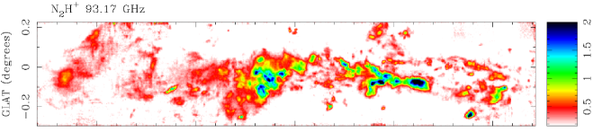
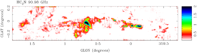
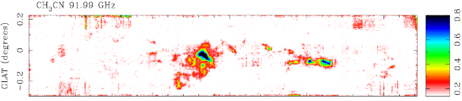
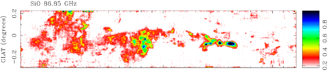
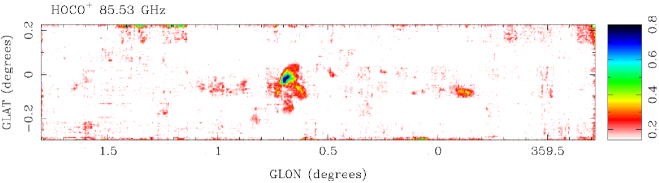
3.2 Peak emission images

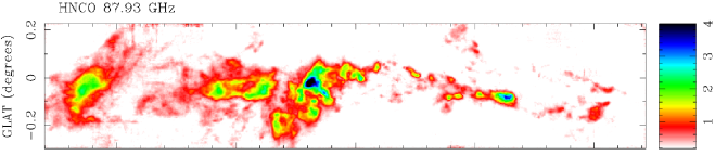
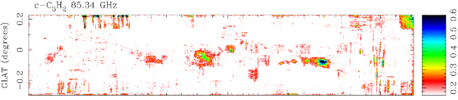
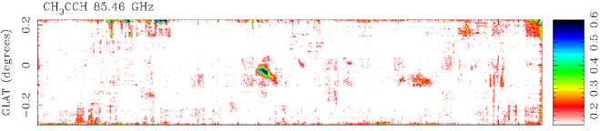
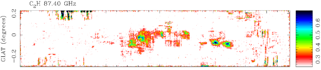
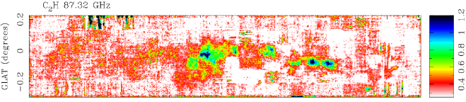
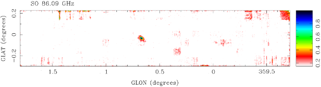
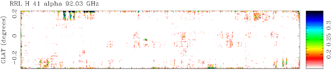
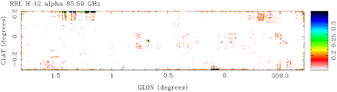
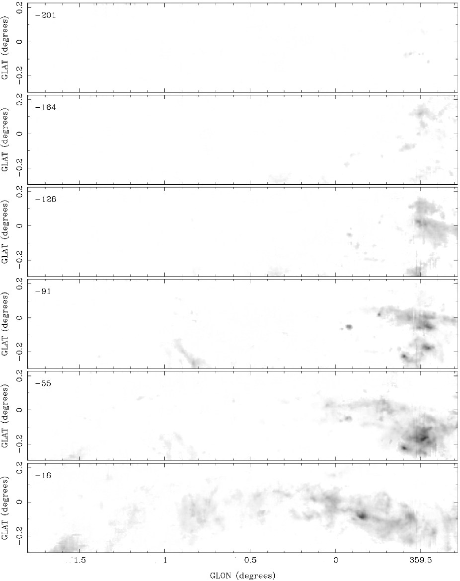
We show the 2-dimensional distribution of the line emission (as listed in Table 1, with quantum numbers) using images of the peak emission in Figs 2 to 5. These images are much more robust to the effect of low level baseline problems than the integrated emission images. They also have the advantage of showing fine structure, being less affected by multiple velocity components. We use the peak brightness within the velocity ranges listed in Table 2. The grey-scale displays start at the 3 $\sigma$ brightness level, so that the display suppresses areas without significant line emission. However, it should be noted that there is emission outside the areas highlighted in these plots, below the 3 $\sigma$ level for individual pixels, which is found to be significant when the data are integrated over larger areas than the beam. That is, when averaging over larger areas, the noise is reduced in terms of brightness, so that weak emission is then clearer above the reduced noise.

We also note that there are some artifacts in some of these peak brightness images, notably stripes in the latitude scanning direction due to data taken in the poorest weather, around $l=1.4$ deg., $b=0.2$ deg. and $l=359.5$ deg., $b=-0.1$ deg.

The peak emission images do not show the line absorption. There is absorption in some stronger lines (e.g HCN, HCO⁺ and HNC) at the strong continuum of Sgr B2 (Jones et al., 2008a) and over a wider area, see subsection 3.3 and Fig. 7. However, the peak emission is mostly not sensitive to this absorption, as the velocities of peak emission are offset from that of the absorbing clouds.

Figure 2: Peak brightness images, for the lines of HCN, HCO⁺, HNC, HNCO, N₂H⁺ and HC₃N. These are the six brightest lines we observed. The grey-scale is peak brightness as $T_{A}^{*}$ in K here and in Figs 3 to 5.

Figure 3: Peak brightness images, for the lines of H¹³CN, H¹³CO⁺, HN¹³C, CH₃CN, SiO and HOCO⁺.

Figure 4: Peak brightness images, for the lines of ¹³CS, c-C₃H₂, CH₃CCH, C₂H and SO.

Figure 5: Peak brightness images, for the H recombination lines.

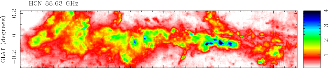
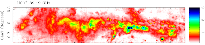
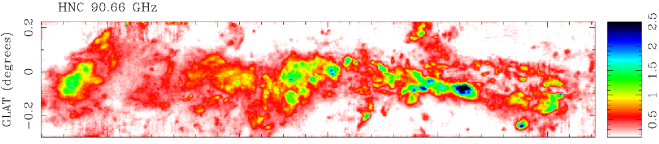
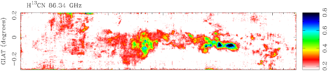
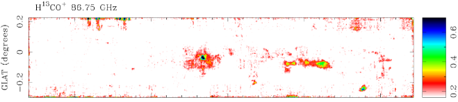
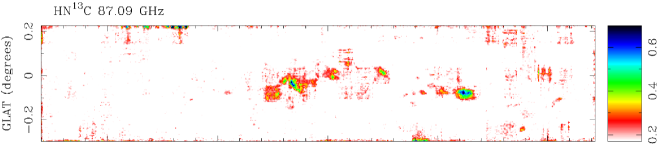
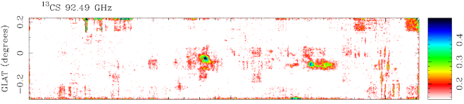
The lines of HCN, HCO⁺ and HNC (Fig. 2) are strong and detected over most of the imaged area. The ¹³C isotopologues, H¹³CN, H¹³CO⁺ and HN¹³C (Fig. 3) are detected in the densest cores, mostly around Sgr B2 and Sgr A. The ratio between these and the HCN, HCO⁺ and HNC lines shows that the latter are optically thick in the densest cores (subsection 3.6). This optical depth effect explains why the position of the brightest peak of HCN, and the velocity of the brightest peak of H¹³CN are different to that of other lines.

Other strong lines that are detected over a large fraction of the CMZ are HNCO, N₂H⁺, HC₃N (Fig. 2), CH₃CN and SiO (Fig. 3). The HNCO and HC₃N peaks are particularly strong around Sgr B2 (Table 2).

Weaker lines that are detected mostly around Sgr B2 and Sgr A are HOCO⁺, ¹³CS, c-C₃H₂,CH₃CCH and C₂H (Fig. 4). The data for the two lines of the C₂H molecule show noise and greater artifacts due to the line frequencies being at the edge of the sub-band, giving poor sensitivity and baseline stability.

The line of SO (Fig. 4) is concentrated at Sgr B2, as are the two radio recombination lines, H 41 $\alpha$ and H 42 $\alpha$ (Fig. 5). These recombination lines indicate significant free-free emission at 3 mm at Sgr B2, as the cascade through Rydberg states of H of recombining electrons occurs under similar conditions to the thermal bremsstrahlung of the free electrons in the ionised gas (Wilson, Rohlfs, Hüttemeister, 2009). The free-free emission component of the Sgr B2 spectrum at 3 mm is also shown by the overall spectral energy distribution (SED) in Jones et al. (2011).

The area around Sgr B2 has interesting differences in the line distributions, which are not well shown at the scale of Figs 2 to 5, but which are shown and discussed in the previous paper Jones et al. (2008a).

3.3 Velocity structure

The line emission in the CMZ spans a large range of velocities (Fig. 1), which, as we note in subsection 3.1, is due to both the large gradient in velocity across the CMZ in the deep potential well of the Galactic Centre and large line widths in the CMZ. We show in Fig. 6 images of the HCN line emission as a function of velocity, integrated over 36 km s^-1 ranges. This demonstrates the large velocity gradient across the Galactic Centre, with negative velocities at more negative longitudes, and positive velocities at more positive longitudes.

The molecular line emission in the CMZ is not symmetrically distributed around the Galactic Centre, so the strongest emission appears at positive longitudes (dominated by Sgr B2 at around longitude $0.7$ degrees) giving an asymmetric distribution in velocity (about $V_{LSR}=0$ km s^-1) in Fig. 6 and the profile in Fig. 1. The area we have observed to cover the strongest emission is longitude $-0.7$ to $1.8$ deg., so there is also some observational selection in this bias to positive longitudes and velocities.

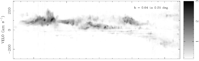
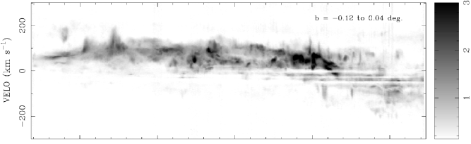
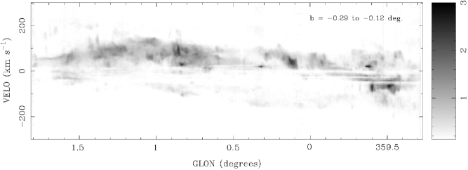
Another way to show the velocity structure is with a position-velocity diagram, as in Fig. 7 for the peak brightness of HCN as a function of velocity and longitude, within three latitude ranges 10 arcmin thick covering -0.29 to 0.21 deg. This shows both the velocity gradient across the region, as well as large velocity widths at some locations.

Also shown in Fig. 7 are absorption features at velocities around $-52$, $-28$ and $-3$ km s^-1, which are also seen in the integrated emission spectrum (Fig.1). These absorption features are clear in the channel images of the HCN data cube, but are not obvious in Fig. 6 because of the large velocity range (36 km s^-1) summed in this plot. Considering the overall Galactic rotation with roughly circular motions around the Galactic Centre, gas along the line of sight to the Galactic Centre will be moving transverse to the line of sight, with zero radial velocity. However, the motions within the Galaxy are not exactly circular, and the absorption features at different velocities are associated with intervening Galactic features (Greaves & Williams, 1994; Wirström et al., 2010). The lines are in absorption, as this intervening low density gas has lower excitation temperature than the background brightness temperature, with excitation temperature $T_{ex}$ of a few K found for CS in sightlines to Sgr B2 by Greaves & Williams (1994).

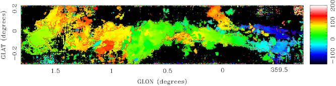
We show in Fig. 8 the image of the peak velocity from N₂H⁺ emission data cube. This line generally shows a well defined peak (see also Fig. 12) and so provides a representation of the principal kinematic velocity at each position in the CMZ. The bulk of the emission peaks at $V_{LSR}\sim+50$ km s^-1, however there is a clear gradient in Galactic longitude of $\sim 200$ km s^-1 evident, extending from $\sim+100$ km s^-1 at $l=+1.5^{\circ}$ to $\sim-100$ km s^-1 at $l=-0.5^{\circ}$. More complex kinematics is also evident. In particular, the twisted cold dust ring noted by Molinari et al. (2011) is apparent in the N₂H⁺ peak velocity image. This elliptical dust ring, $\sim 100\times 60$ pc across, has been hypothesised to trace the location of the system of stable $x_{2}$ orbits in the barred Galactic potential. It is apparent in a dust column density image (see fig. 4 Molinari et al., 2011), and shows a coherent velocity structure as traced in the emission range of the CS 1-0 line (Tsuboi et al., 1999). The kinematics of this ring are more clearly shown in the N₂H⁺ peak velocity image shown in Fig. 8, however. At $l=-0.5^{\circ}$ the western end of the ring is most clearly seen, with velocities smoothly changing from $-20$ to $-100$ km s^-1 around the ring’s extremity. The twist in the ring occurs around $l\sim+0.1^{\circ}$ as it crosses over itself. The eastern side, around $l\sim 0.5-0.8^{\circ}$, is less readily identified in the velocity images, but the emission velocity nevertheless varies smoothly across it, from $20-50$ km s^-1 across the centre of the ring, to $\sim+100$ km s^-1 at its eastern end. The ring twists about the Galactic plane, rising above and below it twice, for one complete orbit. Molinari et al. (2011) propose that this ring is rotating about the centre of the Galaxy with an orbital velocity of 80 km s^-1, tracing the stable, non-intersecting $x_{2}$ orbits whose major axis is perpendicular to that of the Galactic bar, and precesses as the the bar does.

Figure 6: The velocity structure in the CMZ as shown by the HCN line channel images, in 12 panels over 2 pages, averaged over 36 km s^-1 ranges, with the central velocity noted in the top left of each panel. The greyscale range is 0 to 2 K in T${}_{A}^{*}$.

Figure 6 (continued)

Figure 7: Position-velocity diagram of the CMZ, from HCN data, shown as peak brightness temperature, within the three latitude ranges -0.29 to -0.12 deg. (bottom), -0.12 to 0.04 deg. (middle) and 0.04 to 0.21 deg. (top). Note the velocity gradient, and the absorption features at around $-52$, $-28$ and $-3$ km s^-1.

Figure 8: The peak velocity image, from the N₂H⁺ line, with the scale in km s^-1, showing the overall velocity gradient in longitude, but also more complex kinematics. The 0.25 K contour from N₂H⁺ peak brightness is plotted as a guide to the features.

3.4 Integrated line emission

For quantitative analysis of the line data cubes, it is useful to integrate the emission over the velocity range. As the velocity range is large (Table 2 and subsection 3.3 above), the integrated emission images are sensitive to noise and problems with the spectral baselines, as noted in subsection 3.1. This is a well known problem in the analysis of spectral-line data, as discussed for example by van Gorkom & Ekers (1989) and Rupen (1999).

The major problem of simply integrating the emission is spurious stripes, in the longitude and latitude scanning directions, caused by spectral baseline ripples, dominated by the small fraction of data taken during the worst weather. A further problem is that extra noise is added from including parts of the spectra where there is no signal.

A simple method that we adopt here is to integrate the emission above a fixed cutoff level at which the emision is significant. We use a 3-$\sigma$ cutoff, the same used in the peak emission plots (Figs. 2 to 5) to define significant emission. This is quite effective in removing the spurious features in the integrated emission, but not totally effective as the non-gaussian statistics of the baseline errors means there is still a small tail to the distribution of spurious features above the 3 $\sigma$ level. Some of these artifacts can be seen in Figs. 2 to 5.

However, a major problem with this simple method of integration above a cutoff level is a bias in the integrated emission (van Gorkom & Ekers, 1989; Rupen, 1999), with real emission below the cutoff being missed. Because of this, we have investigated two other methods of processing to obtain integrated emission.

An alternative to the fixed cutoff level, is to integrate the emission within a mask defined by the data smoothed spatially and/or over velocity (van Gorkom & Ekers, 1989; Rupen, 1999). We have used as the mask a wavelet reconstruction of the cube, implemented as part of the Duchamp source finding package (Whiting, 2008). This gives a model spectrum at each pixel which contains a range of velocity scales, but not the smallest scale, so has reduced noise, and so can be extended to lower brightness levels than the original data. This gave quite similar results in integrated emission images to the 3-$\sigma$ cutoff version, with slighly more integrated emission, but also slightly more artifacts. It was decided that any improvement was not worth the extra complexity of the processing.

We have also tested different methods of processing the data cubes, with a spectral baseline correction, to give a filtered version, to help the problematic low level ripples. The baseline was determined by an iterative process that clips the data above the 3 $\sigma$ level, replaces these clipped pixels with zero, and then smooths the data with a boxcar filter of width 19 pixels (around 34 km s^-1). The baselines in parts of the data cube with significant emission (above the 3 $\sigma$ level) are unaffected. For parts of the data cube without significant emission, the filtering removes low level offsets to make the mean zero. This is similar to a high order polynomial fit to the spectral baselines (after the exclusion of significant line emission). The baseline corrections are a few times 10 mK, or around half the noise level in the original cubes (Table 2). In practice, the integrated emission determined from the filtered cubes (after a 3-$\sigma$ cutoff, with the reduced level of $\sigma$) was less than that from the unfiltered cubes with the original 3-$\sigma$ cutoff. That is, the effect of integrating to a lower level is overwhelmed by the effect of the filtering biasing the spectra down.

In practice, then, we use the simple integration of emission above a fixed 3-$\sigma$ cutoff level, with the caveat that this will miss some flux from low-level emission. This is a tradeoff to remove the obvious artifiacts. However, since the baseline stability in the data is a limitation, such very low-level broad emission is not measured accurately anyway, so this a limit to the original data, rather than just a problem introduced by the processing.

The integrated emission images show similar features to the the peak emission images Figs. 2 to 5, and look to the eye much like the peak emission images, but with less contrast due to overlapping structures, so are not plotted here.

3.5 Principal Component Analysis

The different spectral lines in the CMZ show similarities as well as differences (Figs. 2 to 5). It would be useful to identify and quantify these features of the data, in a simple objective manner. One useful technique to do so is Principal Component Analysis (PCA), see e.g Heyer & Schloerb (1997).

This describes the multi-dimensional data set by linear combinations of the data that describe the largest variance (the most significant common feature) and successively smaller variances (the next most significant features).

In the context here of integrated emission images, we can use PCA to describe the images, with a smaller set of images which contain the most significant features. This has been used by Ungerechts et al. (1997) for the OMC-1 ridge, and more recently by us for the G333 molecular cloud (Lo et al., 2009) and the Sgr B2 area with 3-mm and 7-mm molecular lines (Jones et al., 2008c, 2011).

We have implemented the PCA processing in a python script, with the PCA module, and pyFITS to read and write the FITS images.

Since the PCA finds features in normalised versions of the different input data sets, it does not work well with low signal to noise data, as the noisy data is scaled up, and the PCA will be dominated by spurious features. So, we restrict our PCA analysis to the strongest eight lines (HCN, HCO⁺, HNC, HNCO, N₂H⁺, SiO, CH₃CN and HC₃N) out of the total twenty lines, and an area around Sgr B2 and Sgr A with the strongest emission. This area was defined by a mask where the integrated emission of the N₂H⁺ line was stronger than 10 K km s^-1. The normalisation of the integrated images makes versions that are mean zero and variance unity.

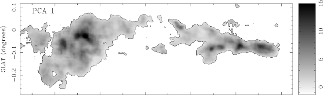
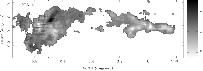
The images of the four most significant components of the integrated emission are shown in Fig. 9. These four components describe respectively 82.6, 10.6, 2.8 and 1.7 percent of the variance in the data. These components are statistical descriptions of the integrated line images, not necessarily physical components of the CMZ. However, they do highlight the physical features in a useful way. The normalised projection of the molecules onto the principal components are shown in Fig. 10 with successive pairs of components.

The first principal component (Fig. 9) shows emission common to all eight strong lines, or a weighted average integrated emission. It describes a large fraction (82.6 percent) of the variance, which means that all eight lines are quite similar in overall morphology. The major features are the ridge of emission in Sgr B2 (Jones et al., 2008a, c) and the dense cores in Sgr A.

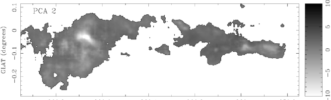
The second principal component (Figs. 9 and 10) shows the major difference (10.6 percent of the variance) among the eight lines, which is differences in the ridge of emission in Sgr B2 and the dense cores in Sgr A, relative to that in the first component. The lines of HCN, HCO⁺, HNC and (to a lesser extent) N₂H⁺ show a relative lack of emission, which we attribute (see below, subsection 3.6) to the brightest areas being optically thick. The other lines (SiO, HNCO, HC₃N and CH₃CN) are, relative to the first component, enhanced at these peaks, which is partly because they are less likely to be optically thick, but it is also likely that these molecules are preferentially found in dense cores.

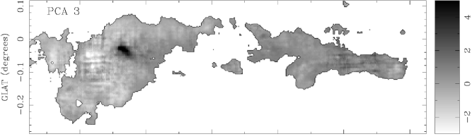
The third principal component (Figs. 9 and 10) shows small differences (2.8 percent of the variance) in the Sgr B2 ridge, between most significantly SiO and HNCO compared to CH₃CN. The fourth principal component shows small differences (1.7 percent of the variance), most significantly between HNCO and SiO. Although the fourth component describes only a small amount of the variance, it is striking that it still appears to have physical significance, as the positive feature corresponds well to the north cloud of Sgr B2 (Jones et al., 2008a, c), where HNCO is enhanced (Minh et al., 1998).

As Sgr B2 is one of the strongest features in the CMZ, and also a chemically complex region, some of the most significant structure in the PCA components here at is in the Sgr B2 region. For PCA analysis of the Sgr B2 area with more lines at 3-mm and 7-mm see Jones et al. (2008c) and Jones et al. (2011) respectively.

Fig. 10 shows the values of the PCA component vectors, for the first four components, plotted as pairs (for convenience of plotting multi-dimensional vectors in two dimensions). These vectors describe how the normalised integrated images of different lines are composed of the sum of different scalar amounts (the components PC 1, PC 2 etc) of the principal component images (Fig. 9). All eight lines have distributions which are made up of positively scaled amounts (PC 1, $\sim$ 0.3) of the first principal component, and further made up of positive or negative amounts (PC 2, etc) of the further principal components.

We also note that the results from PCA analysis (Figs. 9 and 10) are robust to the potential problems of integrating the emission discussed above in subsection 3.4. The PCA components found are almost identical using integrated emission with the 3-$\sigma$ cutoff here, to that from the integrated emission of the baselevel-filtered cubes.

Figure 9: The first four principal component images derived from the eight strongest lines (HCN, HCO⁺, HNC, HNCO, N₂H⁺, SiO, CH₃CN and HC₃N), which describe 82.6, 10.6, 2.8 and 1.7 percent of the variance respectively. The first principal component describes the common features of the eight lines, and the second principal component describes the most significant differences between the lines. The further principal components describe successively smaller differences. As the PCA requires good signal-to-noise data, we have restricted the lines used to the brightest and the area to that defined by the N₂H⁺ emission (see text), as shown by the contour.

Figure 10: The component vectors of the integrated line images in the decomposition of the data into the PCA images, shown with successive pairs of PCA images. HCN, HCO⁺ and HNC have similar vectors so the labels overlap. These vectors describe how the normalised integrated images of different lines are composed of the sum of different scalar amounts of the principal component images (Fig. 9). For example, all eight lines have distributions which are made up of positively scaled amounts (PC 1, $\sim$ 0.3) of the first principal component, but are further made up of positive or negative amounts (PC 2) of the second principal component etc.

3.6 Line Intensities and Line Ratios

The previous subsection (3.5) on PCA shows there are significant differences between the morphology shown by the integrated emission of different lines (at least for the eight strongest lines used for the PCA). One of the most commonly used analysis tools for spectral lines is to consider their line ratios, which we do in this sub-section in order to quantify the behaviour of the principal emitting species further across the CMZ.

The ratio of the integrated emission of the ¹²C to ¹³C isotopologues of HCN, HCO⁺ and HNC lines confirms that the emission of the ¹²C isotopologue is generally optically thick. It is usually much less than 24, the isotopic ratio for [¹²C/¹³C] at the Galactic Centre (Langer & Penzias, 1990), and the value that would be found for optically thin emission. This suggests that the differences in integrated line distribution of HCN, HCO⁺ and HNC, as shown by the second principal component (subsection 3.5, Fig. 9), are related to optical depth effects.

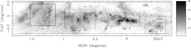
In order to present an analysis for a manageable part of this extensive data set we have obtained on the CMZ we have selected representative regions within the CMZ and examined the line emission through averaged profiles for these apertures. The apertures chosen are listed in Table 3 and plotted in Fig. 11. They include the entire region of the CMZ we have mapped, and the four main emission ‘cores’; Sgr A, Sgr B2, Sgr C and G1.3. We also include a smaller region around the core of Sgr B2. Table 3 lists the centres and sizes of these apertures as well as the velocity ranges chosen for determining the integrated line emission and the line ratios from each aperture. These apertures also provide a basis for comparing the molecular emission from the centre of the Galaxy to that from the central regions of other galaxies, where generally the emission is spatially unresolved and often only the very brightest molecular lines (i.e. from HCN, HNC and HCO⁺) can be seen. We can compare the equivalent parameters found for the entire CMZ, and with the distinct emission regions within it, to examine how they might vary across the central regions of the Galaxy. We can also determine the same parameters in the optically thin isotopologue lines in the CMZ (i.e. H¹³CN, HN¹³C and H¹³CO⁺) to examine whether the optical depth of particular lines may be distorting any interpretation being placed upon a given line ratio.

Table 3: Apertures selected for analysis. The areas are rectangles in Galactic coordinates, centred on $l$ and $b$, and using the velocity ranges indicated to include significant line emission. The projected area on the sky assumes a distance of 8.0 kpc.

Source	$l$	$b$	Width	Height	Area	Area	Min. vel.	Max. vel.
	deg	deg	arcmin	arcmin	arcmin2	pc2	km s-1	km s-1
CMZ	0.545	-0.035	151.0	29.8	4 500	24 400	-220	220
Sgr A	0.040	-0.055	30.8	13.4	413	2 240	-170	220
Sgr B2	0.735	-0.045	29.0	18.2	528	2 860	-130	210
Sgr C	-0.460	-0.145	20.0	17.0	340	1 840	-200	170
G1.3	1.325	0.015	24.2	20.6	499	2 700	-90	220
Sgr B2 Core	0.675	-0.025	6.2	6.2	38	210	-20	200

Figure 11: The six areas selected for analysis: around Sgr A, Sgr B2, Sgr C, G1.3, a smaller area at the Sgr B2 core, and the larger CMZ area, plotted on the peak HCN emission.

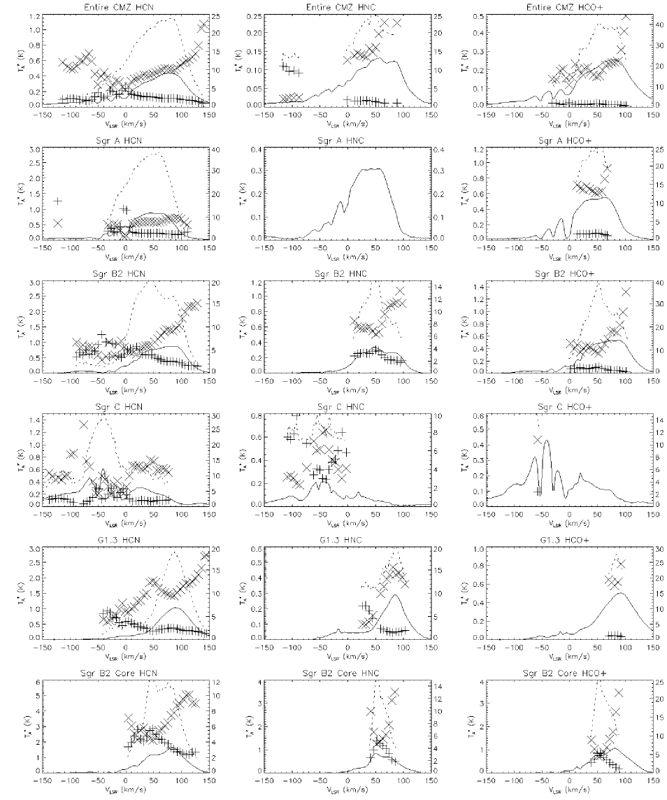
In addition to the HCN, HNC and HCO⁺ lines, as listed in Table 1, there are other bright lines whose distribution is extended across the CMZ. We show the profiles for the CH₃CN, HNCO, HC₃N, N₂H⁺ and SiO lines in Fig. 12, together with those for HCN, HNC and HCO⁺ (and their isotopologues) in Fig. 13. For each aperture the profiles of all lines are rather similar and are very broad (over 100 km s^-1 wide). Some profiles show several absorption features, for instance at $-52$, $-28$ and $-3$ km s^-1 attributable to absorption by cold, foreground gas, likely in spiral arms along the sight line (e.g. as also seen in the AST/RO CO 4–3 datacube of the CMZ; Martin et al. (2004)). The brightest of the lines is HCN, but in some instances other lines are comparably bright (e.g. HNCO in the Sgr B2 Core). The brightness of HCN is generally twice as strong as HCO⁺, the second brightest of these lines, and three times stronger than HNC. Their isotopologue lines are significantly weaker, and we use the ratios with the main lines to derive optical depths in subsection 3.7.

Figure 12: Profiles of five molecular lines in six selected apertures in the CMZ, as defined in Table 3 and Fig. 11. From left to right, the lines are (see Table 1) from the CH₃CN, HNCO, HC₃N, N₂H⁺ and SiO molecules. The apertures run from top to bottom and are: the entire CMZ, Sgr A, Sgr B2, Sgr C, G1.3 and the Sgr B2 Core. Intensities are the averaged pixel values in each aperture, in Kelvin, and are $T_{A}^{*}$ (i.e. without beam efficiency correction). The $x$-axis is the velocity, $V_{LSR}$, running from -200 to +200 km s^-1.

Figure 13: Profiles of the three bright molecular transitions, the HCN, HNC and HCO⁺ J=1-0 lines in the Central Molecular Zone (left, middle and right columns, respectively). Overplotted as dashed lines are the corresponding isotopologues; H¹³CN, HN¹³C and H¹³CO⁺ J=1-0, multiplied by a factor of 3 for clarity. From top to bottom are the six selected apertures (see Table 3 and Fig. 11): the entire CMZ, Sgr A, Sgr B2, Sgr C, G1.3 and Sgr B2 Core. Intensities ($T_{A}^{*}$) are the averaged values over each aperture and velocities are $V_{LSR}$ and run from -250 to +250 km s^-1.

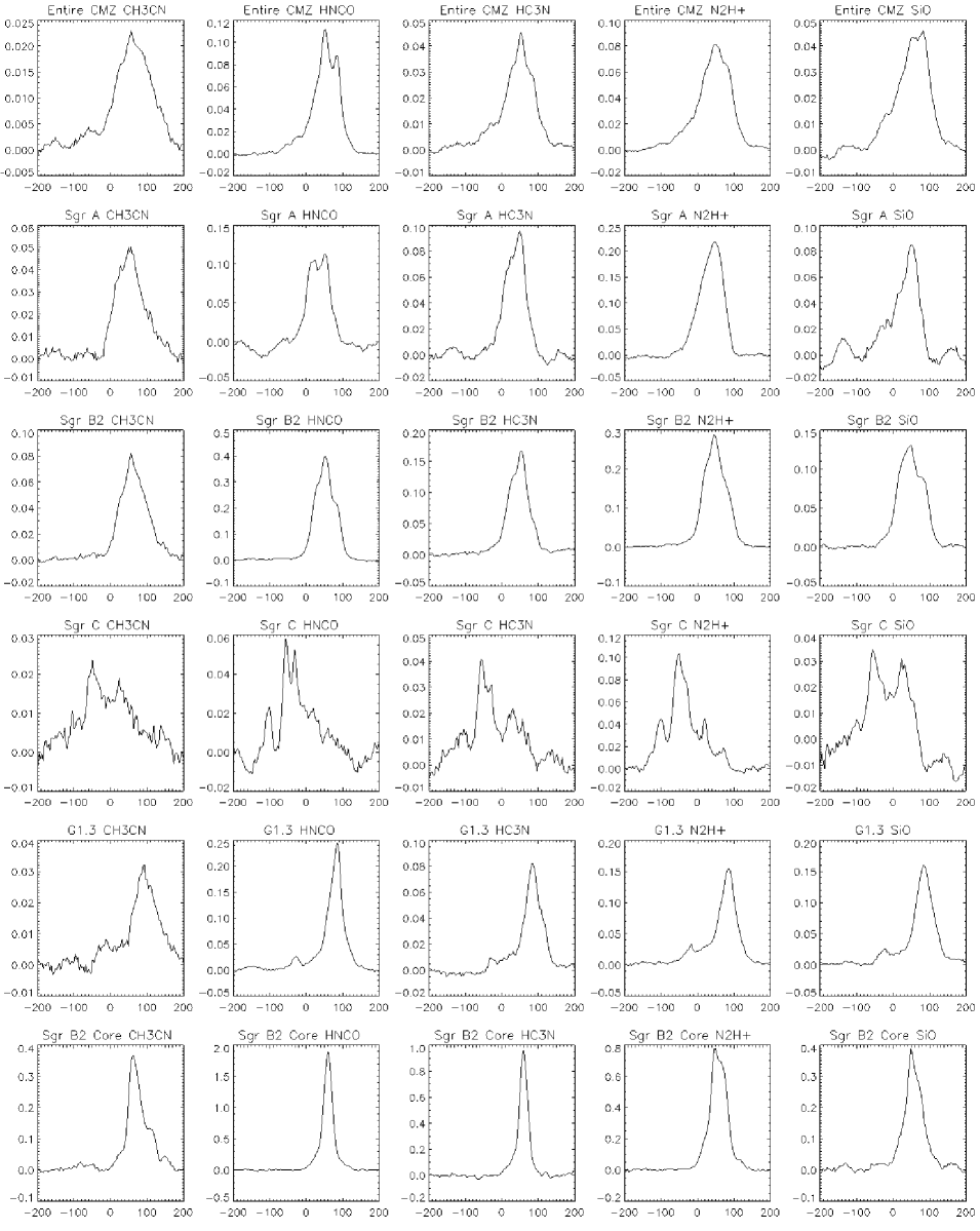
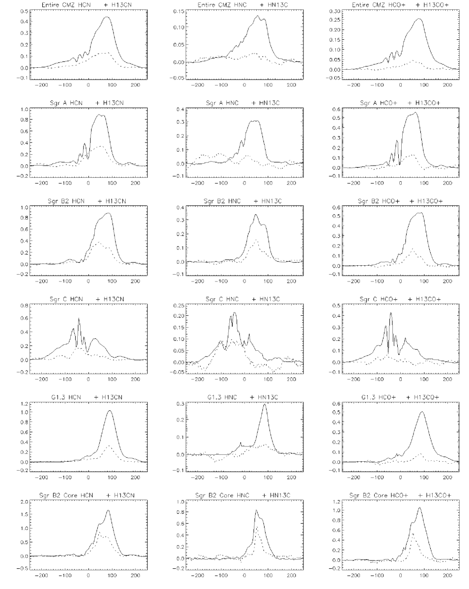
Table 4 presents the integrated line fluxes for these apertures, in K km s^-1 and corrected for the extended aperture efficiency of 0.65 (Ladd et al., 2005). For comparison with extragalactic line luminosities $L^{\prime}$, we integrated the brightness temperatures spatially and spectrally to obtain values in units of K km s^-1 pc² in the different apertures listed in Table 5. As a reference, we also derived $L^{\prime}_{\rm CO}$ using the integrated intensity map of the Columbia survey (Dame, Hartmann, & Thaddeus, Dame et al.). Over the entire CMZ, $L^{\prime}_{\rm CO}$ amounts to $2.2\times 10^{7}$ K km s^-1 pc². Relative to CO, the dense gas tracers exhibit $L^{\prime}_{\rm dense}/L^{\prime}_{\rm CO}$ luminosity ratios of 0.095 (HCN), 0.010 (H¹³CN), 0.029 (HNC), 0.002 (HN¹³C), 0.057 (HCO⁺), 0.002 (H¹³CO⁺), 0.005 (CH₃CN), 0.014 (HNCO), 0.007 (HC₃N), 0.014 (N₂H⁺), and 0.008 (SiO).

Table 6 then presents the relative line ratios with respect to the (brightest) HCN line. The HCN, HNC and HCO⁺ lines may be optically thick, and so to determine whether this influences the derived line ratios we also calculate the isotopologue ratios with H¹³CN in Table 7, alongside the main line ratios with HCN. While the HNC/HCN ratio is found to be roughly the same as HN¹³C/H¹³CN ($\sim$0.3) we find that the HCO⁺/HCN ratio ($\sim$0.6) is typically 2-3 times as high as the H¹³CO⁺/H¹³CN ratio ($\sim$ 0.2-0.3). As we will see below in the analysis of the optical depths, this arises because the HCN line is moderately optically thick (with a similar value to HNC) while the HCO⁺ line has optical depth around unity.

Table 4: Mean integrated line fluxes (K km s^-1), as $\int T_{MB}dV$ (i.e. corrected for aperture efficiency) averaged over the apertures and integrated over the velocity ranges given in Table 3. For each molecule the first line gives the integrated flux and the second line its statistical 1 $\sigma$ error. Note that for the weaker lines the uncertainty in where to place the baseline across the wide line profile means that the formal S/N for the integrated flux is often low, even though the lines themselves are clearly detected. The CO fluxes are obtained from 2001 (Dame et al.).

Source	CO	HCN	H13CN	HNC	HN13C	HCO+	H13CO+	CH3CN	HNCO	HC3N	N2H+	SiO
CMZ	914	87	9	26	2	52	2	4	13	6	13	7
		1	1	1	1	1	1	1	1	1	1	1
Sgr A	1 200	140	18	48	4	85	4	8	10	10	25	9
		1	2	2	4	2	3	2	4	2	2	4
Sgr B2	1 170	142	19	45	5	86	5	11	40	18	33	17
		1	1	2	2	1	1	1	2	1	1	2
Sgr C	1 060	100	9	35	3	61	1	5	5	6	13	3
		2	1	2	3	2	3	1	3	2	1	4
G1.3	1 270	132	12	30	3	73	2	4	20	8	17	17
		1	1	1	1	1	2	1	2	1	1	2
Sgr B2 Core	1 610	199	31	76	11	123	10	33	101	48	68	34
		3	3	5	3	2	4	3	3	3	2	2

Table 5: Line luminosities ($\times 10^{4}$ K km s^-1 pc²), $\int T_{MB}dVdA$ integrated over each aperture and the velocity ranges given in Table 3. For each molecule the first line gives the line luminosity and the second line its statistical 1 $\sigma$ error. Note that for the some lines the uncertainty in where to place the baseline across the wide line profile means that the formal S/N for the luminosity is poor, even though the lines themselves are clearly detected. The CO luminosities are obtained from 2001 (Dame et al.).

Source	CO	HCN	H13CN	HNC	HN13C	HCO+	H13CO+	CH3CN	HNCO	HC3N	N2H+	SiO
CMZ	2 230	212	22	64	5	128	5	11	32	16	32	17
		1	1	2	2	1	2	2	2	1	2	3
Sgr A	268	31.4	4.1	10.8	0.8	19.1	0.9	1.7	2.3	2.1	5.7	2.1
		0.2	0.4	0.5	0.9	0.5	0.8	0.4	0.8	0.3	0.5	0.8
Sgr B2	335	40.6	5.4	12.9	1.5	24.6	1.5	3.1	11.4	5.2	9.3	4.8
		0.3	0.3	0.5	0.5	0.3	0.3	0.3	0.5	0.4	0.2	0.4
Sgr C	195	18.4	1.7	6.4	0.6	11.3	0.2	0.9	1.0	1.1	2.4	0.6
		0.3	0.2	0.3	0.5	0.4	0.5	0.3	0.6	0.3	0.2	0.8
G1.3	343	35.6	3.4	8.0	0.7	19.6	0.5	1.2	5.3	2.2	4.5	4.7
		0.4	0.2	0.3	0.4	0.2	0.5	0.2	0.5	0.3	0.3	0.5
Sgr B2 Core	33.4	4.14	0.64	1.59	0.24	2.56	0.20	0.68	2.09	1.00	1.42	0.71
		0.06	0.06	0.11	0.06	0.05	0.08	0.06	0.06	0.06	0.05	0.05

Table 6: Ratios of integrated lines fluxes with HCN. For each molecule the first line gives the ratio of that line and the HCN 1-0 flux and the second line the 1 $\sigma$ error. For HCN itself the errors indicate the flux error range for that molecule.

Source	HCN	H13CN	HNC	HN13C	HCO+	H13CO+	CH3CN	HNCO	HC3N	N2H+	SiO
CMZ	1.00	0.10	0.30	0.03	0.60	0.03	0.05	0.15	0.07	0. 15	0.08
	0.01	0.01	0.01	0.01	0.01	0.01	0.01	0.01	0.01	0. 01	0.02
Sgr A	1.00	0.13	0.34	0.03	0.61	0.03	0.05	0.08	0.07	0. 18	0.07
	0.01	0.01	0.02	0.03	0.02	0.02	0.01	0.03	0.01	0. 02	0.03
Sgr B2	1.00	0.13	0.32	0.04	0.61	0.04	0.08	0.28	0.13	0. 23	0.12
	0.02	0.01	0.02	0.01	0.01	0.01	0.01	0.01	0.01	0. 01	0.01
Sgr C	1.00	0.09	0.35	0.03	0.61	0.01	0.05	0.05	0.06	0. 13	0.03
	0.04	0.01	0.02	0.03	0.03	0.03	0.01	0.03	0.02	0. 02	0.04
G1.3	1.00	0.09	0.22	0.02	0.55	0.01	0.03	0.15	0.06	0. 13	0.13
	0.02	0.01	0.01	0.01	0.01	0.01	0.01	0.02	0.01	0. 01	0.02
Sgr B2 Core	1.00	0.16	0.38	0.06	0.62	0.05	0.16	0.51	0.24	0. 34	0.17
	0.03	0.02	0.03	0.02	0.02	0.02	0.02	0.02	0.02	0. 02	0.01

Table 7: Ratios of integrated line fluxes for HNC and HCO⁺ with HCN, together with the same ratios measured for their isotopologues.

Source	HNC / HCN	HN13C / H13CN	HCO+ / HCN	H13CO+ / H13CN
CMZ	0.30 $\pm$ 0.01	0.25 $\pm$ 0.10	0.60 $\pm$ 0.01	0.25 $\pm$ 0.09
Sgr A	0.34 $\pm$ 0.02	0.20 $\pm$ 0.24	0.61 $\pm$ 0.02	0.23 $\pm$ 0.22
Sgr B2	0.32 $\pm$ 0.02	0.28 $\pm$ 0.11	0.61 $\pm$ 0.01	0.27 $\pm$ 0.08
Sgr C	0.35 $\pm$ 0.02	0.35 $\pm$ 0.34	0.61 $\pm$ 0.03	0.11 $\pm$ 0.29
G1.3	0.22 $\pm$ 0.01	0.22 $\pm$ 0.12	0.55 $\pm$ 0.01	0.15 $\pm$ 0.17
Sgr B2 Core	0.38 $\pm$ 0.03	0.37 $\pm$ 0.13	0.62 $\pm$ 0.02	0.31 $\pm$ 0.15

Molecules like CH₃CN, HNCO and HC₃N and N₂H⁺ are generally found in dense molecular cores or cold dust cores where massive star formation has recently been initiated. The ratios of the lines from these molecules to HCN (Table 6) is seen to be more variable between the apertures than they are for HNC and HCO⁺, with, in particular, Sgr B2 showing significantly larger values of the ratios than the other locations (typically 3-5 times larger). SiO, which is more sensitive to the presence of shocks, shows less variation between the apertures, but still has a ratio twice as large for Sgr B2 as in Sgr A and Sgr C. However G1.3 has a similar ratio to Sgr B2, suggesting the influence of shocks in this region too.

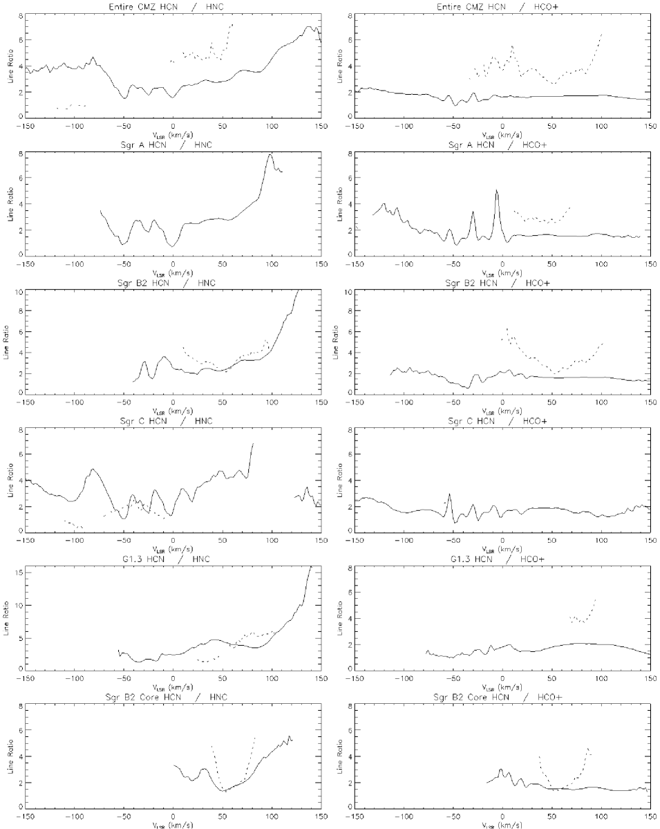
Table 8 lists the maximum and minimum line ratios found for HCN, HNC and HCO⁺, as well as for their ¹³C isotopologues, as a function of velocity between the apertures, as opposed to the integrated line fluxes. The variations between these extrema can be seen in Fig. 14 (note that line ratios are only shown when the individual lines have S/N $>5$ for a given velocity channel). Within the core of each line the ratios are generally constant, aside from the velocity ranges where foreground absorption is evident (see above). The isotopologue line ratios are generally similar for H¹³CN / HN¹³C compared to HCN/HNC. However for H¹³CN / H¹³CO⁺ the isotopologue line ratio is typically twice the value of HCN/HCO⁺, as the velocity varies. This result, for the variation in ratio as a function of velocity, is also consistent with behaviour found for the ratio of the integrated fluxes of these lines.

However, at the highest red-shifted velocities for emission ($>100$ km s^-1), the behaviour changes, with the ratio HCN / HNC increasing significantly, from a value of $\sim 2$ over most of the profile, to $\sim 10$ at its high-velocity limit. This trend is also apparent in the ¹³C forms, H¹³CN/HN¹³C, though lower S/N limits the velocity range over which the comparison may be made. We note, however, that the HCN / HCO⁺ ratio does not show any evidence for increasing at these high red-shifted velocities, suggesting that this variation is a result of the relative strength of the HNC line decreasing with increasing velocity, while the relative intensity of the HCN and HCO⁺ lines remains constant.

Table 8: Maximum and minimum values of selected line ratios with the velocities ($V_{LSR}$) at which these extrema occur. Note that line intensities need to be $>5\sigma$ per channel to be used for this analysis. No data meets this criteria for HN¹³C in Sgr A.

Source	HCN / HNC				H13CN / HN 13C				HCN / HCO+				H13CN / H13CO+
	Max.	Vel.	Min.	Vel.	Max.	Vel.	Min.	Vel.	Max.	Vel.	Min.	Vel.	Max.	Vel.	Min.	Vel.
	ratio	kms-1	ratio	kms-1	ratio	kms-1	ratio	kms-1	ratio	kms-1	ratio	kms-1	ratio	kms-1	ratio	kms-1
CMZ	7.5	183	1.5	-49	8.2	77	0.7	-116	2.5	-192	0. 9	223	6.6	101	2.6	52
Sgr A	7.8	97	0.7	-1	-	-	-	-	5.1	-7	0. 9	-47	3.8	68	2.6	45
Sgr B2	9.9	127	1.2	-41	5.3	94	2.2	54	2.6	-94	0. 6	-36	6.3	4	2.0	54
Sgr C	6.8	81	1.1	-50	2.5	-39	0.4	-92	3.0	-54	0. 7	-49	2.5	-56	2.3	-59
G1.3	15.9	139	1.3	-34	6.2	101	1.4	34	2.1	75	1. 0	212	5.4	94	3.7	70
Sgr B2 Core	5.6	117	1.4	50	5.5	86	1.3	54	3.0	-1	1. 3	143	4.7	86	1.4	52

Figure 14: Line ratios, as a function of velocity, for HCN/HNC (left) and HCN/HCO⁺ (right), for the six selected apertures in Table 3 (the entire CMZ, Sgr A, Sgr B2, Sgr C, G1.3 and the Sgr B2 Core). The main line is shown in solid and the ¹³C–isotopologue ratios (H¹³CN/HN¹³C and H¹³CN/H¹³CO⁺) are dashed. Line ratios are only shown when the intensities of both lines are $>5~{}\sigma$ in the relevant velocity channel. Note that for HN¹³C in Sgr A this results in no useable isotopologue data (and just 2 data points for H¹³CO⁺ in Sgr C). The $x$-axis is the $V_{LSR}$ velocity, running from -150 to +150 km s^-1. Note that the $y$-axis ranges are the same in all plots except for Sgr B2 and G1.3 (left column).

3.7 Optical Depth Analysis

Table 9: Maximum and minimum values of the ratios of the line intensities, per velocity channel, for HCN, HNC and HCO⁺ with their ¹³C isotopologues, together with the velocities ($V_{LSR}$) at which these extrema occur. Note that all line intensities need to be $>5\sigma$ per channel to be used for this analysis. No data meets this criteria for HN¹³C in Sgr A.

Source	HCN / H13CN				HNC / HN13C				HCO+ / H13CO+
	Max.	Vel.	Min.	Vel.	Max.	Vel.	Min.	Vel.	Max.	Vel.	Min.	Vel.
	ratio	km s-1	ratio	km s-1	ratio	km s-1	ratio	km s-1	ratio	km s-1	ratio	km s-1
CMZ	22.3	139	4.6	-1	23.3	77	2.1	-114	44.1	101	1 0.1	-28
Sgr A	11.1	-37	1.5	-1	-	-	-	-	20.3	68	1 2.4	46
Sgr B2	15.8	127	2.6	-47	14.1	94	6.2	52	38.6	103	8.4	52
Sgr C	29.9	-78	2.9	-54	8.9	-39	2.2	-83	14.2	-59	7.0	-56
G1.3	18.9	143	3.3	-36	16.4	81	3.1	26	27.4	94	1 6.6	83
Sgr B2 Core	10.4	110	4.1	46	13.9	83	4.4	54	22.3	86	4.0	52

Where the H¹³CN, HN¹³C and H¹³CO⁺ lines are well detected (S/N $>5$) we may use the ratio with the main isotopologue to determine the optical depth of the emission, as a function of velocity across the line ratio. We list in Table 9 the maximum and minimum values of the ratios found for the isotopologue pairs (i.e. HCN/H¹³CN, HNC/HN¹³C and HCO⁺/H¹³CO⁺) across their line profiles, together with the velocities at which these extrema occur. Again, these numbers are filtered to require the S/N in each velocity channel to be $>5\sigma$. The variation of each line ratio with velocity can be followed in Fig. 15. The ratios are generally well less than 24, the abundance ratio for ¹²C to ¹³C determined for the centre of the Galaxy (Langer & Penzias, 1990), indicating that the ¹²C isotopologues of these species must be optically thick. However, the isotopologue ratios are also significantly greater than unity, which also implies that the ¹³C lines cannot be strongly optically thick. We make use of this behaviour to provide an approximate solution of the radiation transfer equation below. We apply a standard analysis technique, which we summarise here.

The radiative transfer equation has the general solution for the intensity of a velocity channel in a spectral line known as the detection equation (e.g. Stahler & Palla, 2005):

$$T_{A}=T_{A}^{*}/\eta=f[J_{\nu}(T_{ex})-J_{\nu}(T_{BG})](1-\exp(-\tau_{\nu}))$$

where $T_{A}^{*}$ is the measured intensity, $\eta$ the extended beam efficiency (taken as 0.65, Ladd et al., 2005). $f$ is the beam filling factor for the emission, $J_{\nu}(T)=[h\nu/k]/[\exp(h\nu/kT)-1]$, with $T_{ex}$ being the excitation temperature and $T_{BG}$ being the temperature of the CMBR (i.e. 2.726 K). $\tau_{\nu}$ is the optical depth of the emission.

For a line isotopologue pair, say HCN and H¹³CN, we assume the former is optically thick, but the latter is optically thin, as inferred above. We also assume they have the same excitation temperature and beam filling factor. Furthermore,

$$\tau_{HCN}/\tau_{H^{13}CN}=N(HCN)/N(H^{13}CN)=X_{{}^{12}C/^{13}C}$$

the abundance ratio of the ¹²C isotope to ¹³C, which we have taken to be 24 (Langer & Penzias, 1990), assuming no isotope fractionation in the molecules.

Then we see, from application of the detection equation to HCN and H¹³CN, that $\tau_{H^{13}CN}=T_{A}^{*}(H^{13}CN)/T_{A}^{*}(HCN)$, with $\tau_{HCN}$ then determined by the preceding formula.

We hence apply this analysis to determine the optical depth of the HCN, HNC and HCO⁺ lines, as a function of velocity. Furthermore, from standard molecular radiative transfer theory (e.g. Goldsmith & Langer, 1999) we may show that the column density of the upper level of each transition is given by

$$N_{u}=[8\pi k/Ah][\nu^{2}/c^{3}]T_{A}[\tau/1-\exp(-\tau)]\delta V$$

where $k$, $h$ and $c$ are the well-known physical constants, $\nu$ is the frequency of the transition, $A$ its radiative decay rate (Einstein coefficient) and $\delta V$ the channel velocity spacing. The optically thin case ($\tau\ll 1$) simply has the optical depth correction factor $\tau/(1-\exp(-\tau))$ set to unity.

Once $N_{u}$ has been determined the total molecular column density $N$ can be found by applying $N=(N_{u}Q(T)/g_{u})\exp(E/kT_{ex})$ with $g_{u}=2J+1=3$, the partition function $Q(T)=2kT/h\nu$, $E$ the energy of the upper level and an assumed excitation temperature, $T_{ex}$. We take the later as 24 K, based on the dust temperature of the Sgr B2 envelope (Jones et al., 2011). Nagayama et al. (2009) determined that $T_{ex}$ has the range 20 to 35 K in the CMZ from LVG modelling of the CO lines. To check the sensitivity of this assumption we also repeated our calculations by halving and doubling the temperature. For the former (i.e. $T=12$ K) the column densities (and masses) decrease by a factor $\sim 0.6$. For the latter (i.e. $T=48$ K) they increase by a factor $\sim 1.8$. While undoubtedly variations in the excitation temperature across the CMZ could result in relative variations in these calculated quantities by factors of a few, the absolute determinations for the column density in each aperture are not likely to be in error by more than a factor 2 due to this assumption of a constant temperature $T=24$ K

Similarly the molecule mass $M$ can then be determined from the column density $N$ knowing the aperture size (Table 3), molecular masses $m_{mol}$, and the source distance ($D=8.0$ kpc) as $M=Nm_{mol}\Omega D^{2}$.

In Table 10 we list the derived optical depths for each aperture for HCN, HNC and HCO⁺. We list both the maximum value of the optical depth found at each position (together with the relevant emission velocity) and the weighted mean optical depth. This is determined from the value of the correction factor $\tau/(1-\exp(-\tau))$ needed to convert the integrated line flux from that for an optically thin line to the measured integrated line flux after applying the optical depth correction at each velocity channel. This number thus provides a representative value of the optical depth for each line. For HCN and HNC this is typically 2-3, whereas for HCO⁺ it is around unity. On the other hand, the maximum values of the optical depth for each line are several times their mean values. These are illustrated graphically in Fig. 15. This shows, for each source and line, both the measured and the optical-depth corrected line profile. Also shown, with the right-axis as the numerical value, are the measured value of the isotopologue line ratio (i.e. HCN/H¹³CN etc.) and the value determined for the optical depth at each velocity. The optical depth is found to be fairly constant over each line though note that it is higher where the absorption features are seen; however by applying the optical depth correction these features are removed from the line profiles, as can be seen by their smoothly passing across the affected velocities in Fig. 15.

Table 10: Optical depths, for HCN, HNC, and HCO⁺, derived from the isotopologue ratios assuming [¹²C/¹³C] = 24, given as the maximum and the weighted mean. The velocity listed is that at which the maximum optical depth occurs. See the text for the definition of the weighted mean value of the optical depth.

Source	HCN	HCN	HCN	HNC	HNC	HNC	HCO+	HCO+	HCO+
	Max.	Vel.	Mean	Max.	Vel.	Mean	Max.	Vel.	Mea n
	$\tau$	km s-1	$\tau$	$\tau$	km s-1	$\tau$	$\tau$	km s-1	$\tau$
CMZ	5.2	-1.1	2.4	11.7	-114.1	1.0	2.4	-28.4	0.9
Sgr A	16.5	-1.1	3.0	-	-	-	1.9	46.3	1.0
Sgr B2	9.1	-46.6	3.2	3.9	51.8	2.5	2.9	51.8	1.4
Sgr C	8.2	-52.1	2.2	11.0	-83.1	2.9	3.4	-55.8	0.1
G1.3	7.4	-35.7	2.2	7.6	26.3	1.6	1.4	82.8	0.4
Sgr B2 Core	5.9	46.3	3.6	5.5	53.6	2.6	5.9	51.8	2.0

Figure 15: Optical depth-corrected line intensities, together with the optical depth and isotopologue ratios, as a function of velocity. From left to right are the HCN, HNC and HCO⁺ measured line profiles (solid line) and optically-depth corrected profile (dashed line). The intensity, $T_{A}^{*}$, in Kelvin is shown on the left-hand axis, and the $x$-axis shows the velocity in $V_{LSR}$ from $-150$ to $+150$ km s^-1. The symbol $\times$ shows the measured isotopologue line ratio for each molecule (i.e. HCN/H¹³CN, HNC/HN¹³C and HCO⁺/H¹³CO⁺) and the $+$ sign shows the calculated optical depth for the HCN, HNC and HCO⁺ J=1-0 lines, respectively (see text). The right-hand axis indicates the numerical value for the line ratio and optical depth. The six selected apertures (see Table 3) are, from top to bottom, the entire CMZ, Sgr A, Sgr B2, Sgr C, G1.3 and the Sgr B2 Core. Note that optical depths and line ratios are only calculated when the corresponding lines are $>5~{}\sigma$ (i.e. HCN and H¹³CN $>5~{}\sigma$, etc.). For some lines/sources (e.g. HN¹³C in Sgr A) there are few, or no, data for which this condition is met. Also, for clarity, every three data points in the $x$-direction are binned together to provide a single point on the plots.

While the isotopologue line ratios are not found to vary much over the cores or blue-wings of each line, this is not the case for the red-shifted gas, however. For several apertures (especially the entire CMZ, Sgr B2 and G1.3; see Fig. 15) these ratios rise steeply for velocities $>+50$ km s^-1, from values of $\sim 5$ to reach 20–40 for the most red-shifted emission (see also Table 9; note that this analysis has only been applied to data with S/N $>5$ per channel so this is not an artifact of low S/N at the profile edges). This is as expected if the optical depth is falling with increasing velocity, with the line ratio tending towards the optically thin value given by the [¹²C/¹³C] isotope ratio. However, we note that the ratios determined for the entire CMZ and Sgr B2 for the HCO⁺ isotopologues at the highest velocities are $>30$, greater than the assumed isotope abundance ratio of 24 for the CMZ. We discuss this further in subsection 4.3.

Finally Table 11 presents the derived column density and masses for each aperture and molecule. Presented here are the upper level column density, without any optical depth correction, and the total molecule column density, correcting for optical depth and assuming an excitation temperature of 24 K. The molecule masses are then derived for each aperture from the total column density for that molecule. The column densities for each molecule vary little with aperture, though of course the masses do as they are summed over the aperture. Around 50 M_⊙ of [HCN+HNC+HCO⁺] exists in the CMZ, 60 percent of this being HCN and 20 percent each HNC and HCO⁺. Furthermore, 10-15 percent of the total mass of the CMZ is associated with each of the regions Sgr A, Sgr B2 and G1.3.

We end this section by noting that we have considered calculating the molecule abundances by making use of the sub-millimetre dust data to provide total column densities in each aperture, and then ratioing these values with the relevant molecular column densities. Three such data sets have been published, at 1.1 mm (BOLOCAM, Bally et al., 2010), at 450 and 850$\mu$m (SCUBA, Pierce-Price et al., 2000) and at 870$\mu$m (LABOCA, Schuller et al., 2009). However close examination of these data sets reveals issues with the determination of the baseline in an extended emission region such as the CMZ, given the data acquisition methods applied. Significant levels of low-level emission are missing in the final images, so yielding incorrect dust column determinations, even before other uncertainties such as dust temperature and opacities are considered. We have therefore not attempted to determine molecular abundances from our data set, which await further work on the analysis of the extended dust emission across the CMZ before reliable values can be calculated.

Table 11: Column density and mass for HCN, HNC and HCO⁺. The column densities are the mean over each aperture, and calculated as $N_{J=1}$, in the $J=1$ level without the correction for optical depth and, as $N$ the sum over all levels, with the correction for optical depth ($\tau/(1-\exp(-\tau))$), applied per velocity channel and assuming $T_{ex}=24$ K. The mass, $M$, is the sum over the aperture defined in Table 3, calculated including the correction for optical depth. Note if $T_{ex}$ is halved $N$ and $M$ decrease by 0.6 times, while if $T_{ex}$ is doubled they increase by 1.8 times.

Source	$N_{J=1}$	$N$	$M$	$N_{J=1}$	$N$	$M$	$N_{J=1}$	$N$	$M$
	HCN	HCN	HCN	HNC	HNC	HNC	HCO+	HCO+	HCO+
	no corr.	corr.	corr.	no corr.	corr.	corr.	no corr.	corr.	corr.
	1014 cm-2	1014 cm-2	M☉	1014 cm-2	1014 cm-2	M☉	1014 cm-2	1014 cm-2	M☉
CMZ	1.5	17	29	1.0	7.0	11	0.74	5.0	8.8
Sgr A	1.6	23	3.5	0.96	4.2	0.64	0.72	5.1	0.81
Sgr B2	1.7	25	4.8	0.84	9.9	1.9	0.74	6.3	1.3
Sgr C	1.4	15	1.9	0.90	12	1.5	0.60	2.8	0.37
G1.3	1.4	16	2.9	0.61	5.4	0.98	0.65	3.5	0.68
Sgr B2 Core	1.8	31	0.43	0.84	11	0.15	0.76	7.9	0.12

4 Discussion

4.1 CMZ Line Luminosities Compared to External Galaxies

Gao & Solomon (2004) surveyed 52 galaxies in HCN(1-0) that were selected to cover a large range of FIR luminosities. Their sample galaxies show $L^{\prime}_{\rm CO}$ values in the $5\times 10^{8}$ to $1.5\times 10^{10}$ K km s^-1 pc² range. This is considerably more than what is measured in the CMZ. Even galaxies that are considered Milky Way equivalents, such as IC 342, show over an order of magnitude larger $L^{\prime}_{\rm CO}$ luminosities. The reason for the difference is likely the edge-on orientation of the CMZ, the sample selection that picks galaxies with rather large FIR fluxes, as well as the fact that the physical size of their single dish beam projects to kpc size scales at the distances of the sample galaxies – much larger than the $\sim$350 pc of our CMZ image. The ratio of $L^{\prime}_{\rm HCN}/L^{\prime}_{\rm CO}$ in the Gao & Solomon (2004) sample, however, is in the range 0.03 - 0.18, which is very similar to what we find in the CMZ (0.095). This is also in agreement with the more recent observation of Krips et al. (2008). They observed a sample of 12 nearby, starburst and active galaxies and derive $L^{\prime}_{\rm HCN}/L^{\prime}_{\rm CO}$ luminosity ratios of 0.1-0.5 for the bulk of their sample of 12 galaxies. The CMZ is at the lower end of that range and may indicate that the star formation activity correlates with the availability of dense gas relative to CO, a trend established by Solomon, Downes & Radford (1992) and Gao & Solomon (2004) and interpreted, e.g., by Krumholz, McKee & Tumlinson (2009). Krips et al. (2008) also measure HCO⁺ and they derive $L^{\prime}_{\rm HCO^{+}}/L^{\prime}_{\rm HCN}$ ratio in the 0.5 to 1.6 range. Our value for the CMZ is with 0.6, at the lower end of that distribution.

4.2 Interpreting Line Ratio Variations for HCN, HNC and HCO⁺ in External Galaxies

The ratios of the fluxes of the HCO⁺, HCN and HNC lines are often measured in studies of extra-galactic sources, where they may provide the only readily accessible probe of the dense molecular environment across the entire central regions of a Galaxy (e.g. Loenen et al., 2008). In particular, the ratios of these lines have been used to distinguish X-ray-dominated regions (XDRs) from photodissociation regions (PDRs) (Meijerink, Spaans, & Israel, Meijerink et al.2007), and applied to starburst galaxies (Baan et al., 2008).

The spatially resolved ratios for these lines that we have determined from the CMZ are therefore useful in providing a Galactic analogue to compare such results with. Within the CMZ it is possible to study how the ratio may change with position, due to changing excitation conditions, as well as to see how it appears when blended together in a single pixel as in an external galactic nucleus. We may also examine the effects of opacity on the diagnostic line ratios by comparing them to the ratio obtained using their optically thin isotopologues. The isotopologues may not be measurable in an external galaxy due to their weakness, yet excitation conditions may be also mis-diagnosed if the measured line ratios do not reflect the intrinsic line ratio due to one line of a pair being more affected by optical depth than the other.

In such analyses of external galaxies generally the logarithm of the line ratios (e.g. log[I(HCO⁺)/I(HCN)] etc.) is presented. To aid this comparison we have therefore re-calculated the line ratios in Table 7 into their logarithm values and present these in Table 12, together with the errors. For completeness we have also included HCO⁺/HNC in this table although it can be calculated from the other two ratios. The value for the ¹³C line ratios in Table 12 can be interpreted as providing the optically thin ratio for the corresponding ¹²C line ratios across the CMZ.

For log(HNC/HCN) the line ratio varies from $-0.4$ to $-0.6$ between the apertures. The ¹³C line ratios are consistent with those for the corresponding ¹²C value, within the errors of measurement. However, this is not the case for log(HCO⁺/HCN). This varies little between the 6 apertures we have chosen for the ¹²C line ratios, from $-0.21$ to $-0.26$. Yet for the ¹³C isotopologues the corresponding value is typically a factor 2 higher (i.e. ranging from $-0.5$ to $-0.6$). For log(HCO⁺/HNC) there is a factor of 2 variation measured between the apertures, from 0.2 to 0.4. However, while the measured ¹³C isotopologue ratios for these species may appear to differ from this in Table 12, the relevant lines are too weak to discern any significant difference from the corresponding ¹²C ratios. To summarise, the empirical result from the CMZ data presented here is that the HCO⁺/HCN ratio needs to be determined from measurements of the ¹³C isotopologues, but the HNC/HCN ratio can be determined using the main ¹²C lines. We cannot determine whether the ¹³C isotopologues are necessary to measure the true HCO⁺/HNC ratios. However the analysis given earlier, showing that the HCO⁺ optical depth is generally less than that for HNC, suggests that this is likely to be the case.

Loenen et al. (2008) examine the HCN, HNC and HCO⁺ line ratios in a number of IR-luminous galaxies and present plots of their variation for the three ¹²C-species ratios considered in Table 12. They discriminate in these plots between excitation regimes dominated by PDRs from XDRs; HNC and HCO⁺ are found to be relatively stronger, compared to HCN, in XDRs than PDRs. They find that nearly all the sources they studied lie clearly in the PDR-regime; indeed they need to invoke an additional heating source (“mechanical heating”) even to explain the ratios under the PDR regime.

Applying the results from our CMZ study actually exacerbates this situation. All points for the CMZ also lie clearly in the PDR regime in these plots (see Fig. 1 of Loenen et al., 2008), which is not unexpected given the $\rm 10^{7}L_{\odot}$ IR luminosity of the CMZ is dominated by re-processed dust emission. The CMZ data points lie in the same region of the phase space in these diagrams as the majority of the galaxies in the study. However, applying the H¹³CO⁺/H¹³CN ratio as a diagnostic, instead of HCO⁺/HCN, moves the CMZ points even further from the dividing line between the PDR and XDR regimes. By analogy, this suggests that this is also likely to be the case for the majority of galaxies where these diagnostic ratios have been measured.

Table 12: Logarithm of line ratios, for the integrated flux through each aperture, for HCN, HNC and HCO⁺, together with same ratios measured for the ¹³C isotopologue. Statistical errors are also listed for each ratio.

Source	log(HCO+/HCN)	log(H13CO+/H13CN)	log(HNC/HCN)	log(HN13C/H13CN)	log(HCO+/HNC)	log(H13CO+/HN13C)
CMZ	$-0.22\pm 0.01$	$-0.59\pm 0.13$	$-0.52\pm 0.02$	$-0.61\pm 0.16$	$+0.30\pm 0.02$	$+0.02\pm 0.21$
Sgr A	$-0.22\pm 0.02$	$-0.64\pm 0.29$	$-0.46\pm 0.03$	$-0.70\pm 0.35$	$+0.25\pm 0.04$	$+0.06\pm 0.47$
Sgr B2	$-0.22\pm 0.01$	$-0.57\pm 0.11$	$-0.50\pm 0.03$	$-0.54\pm 0.14$	$+0.28\pm 0.03$	$-0.02\pm 0.20$
Sgr C	$-0.21\pm 0.04$	$-0.97\pm 0.57$	$-0.46\pm 0.04$	$-0.45\pm 0.30$	$+0.25\pm 0.05$	$-0.52\pm 0.65$
G1.3	$-0.26\pm 0.02$	$-0.83\pm 0.33$	$-0.65\pm 0.03$	$-0.67\pm 0.21$	$+0.39\pm 0.03$	$-0.15\pm 0.42$
Sgr B2 Core	$-0.21\pm 0.03$	$-0.50\pm 0.18$	$-0.42\pm 0.05$	$-0.43\pm 0.14$	$+0.21\pm 0.05$	$-0.07\pm 0.22$

4.3 Isotopologue Line Ratio Variations with Velocity

As can be seen in Fig. 15 and was discussed in subsection 3.7 the line ratios for the three isotopologue pairs increase significantly with red-shifted velocity in several locations (CMZ, Sgr B2, G1.3). The trend is particularly noticeable for HCO⁺ and HCN, and less so for HNC. This can be caused by decreasing optical depth of the ¹²C species with increasing velocity, with the line ratio then tending towards the [¹²C/¹³C] isotope ratio (at least in the absence of fractionation effects). However we note that there is no trend of increasing ratio (or decreasing optical depth) seen to the blue-shifted side of the line profiles.

Of the three line ratio pairs, the HCO⁺/H¹³CO⁺ ratio is generally the highest. This is also consistent with the average optical depth of the HCO⁺ line being lower than HCN or HNC (see Table 10). HCO⁺ provides, therefore, the best probe of the optically thin ratio; i.e. of the [¹²C/¹³C] isotope ratio.

For the Sgr B2 and integrated CMZ apertures the HCO⁺/H¹³CO⁺ ratio rises as high as $\sim 40$ at the high-velocity edge of the profile, considerably in excess of the [¹²C/¹³C] average isotope ratio of 24 for the centre of the Galaxy. Taken by itself, the rising ratio with decreasing HCO⁺ intensity in the red-shifted wing could be a result of a systematic error in the baseline subtraction of the ¹³C species, making the calculated flux relatively fainter compared to the ¹²C species than it should be. However a similar result has also been reported by Riquelme et al. (2010b) in the Galactic Centre from observations using the IRAM 30m telescope. They find similarly high HCO⁺/H¹³CO⁺ ratios ($\sim 40$) at several selected positions in the central $5^{\circ}$ of the Galaxy, with the ratio also highest for the most red-shifted gas. Riquelme et al. (2010b) also measure lower values for the HCN and HNC isotopologue ratios, similar to our results.

If these inferred isotope ratios of $>24$ are correct then this red-shifted gas has undergone a different degree of nuclear processing that the bulk of the CMZ gas, which has a [¹²C/¹³C] isotope ratio of 24. ¹²C is primarily produced in first generation, massive stars on a rapid timescale. ¹³C arises from CNO processing of ¹²C in lower mass stars, on a slower time-scale (e.g. Prantzos, Aubert, & Audouze, 1996). There is also a gradient in [¹²C/¹³C] observed with distance from the centre of the Galaxy, rising from $\sim 24$ there to reach 80-90 in the solar neighbourhood (Wilson, 1999). Riquelme et al. (2010b) interpret these elevated isotope ratios resulting from infall of material to the centre of the Galaxy. Positions observed associated with $x_{1}$ orbits (which are parallel to the Bar) had higher inferred values of [¹²C/¹³C] than those positions associated with $x_{2}$ orbits (which are inside and orthogonal to the $x_{1}$ orbits; see Stark et al. (2004)).

There is limited overlap between the positions observed by Riquelme et al. (2010b) and ourselves; moreover the large apertures we have used for our analysis are in contrast to the single beams used by Riquelme et al. (2010b). Nevertheless, the Sgr B2 aperture we applied includes both a position at high-velocity associated with an $x_{1}$ orbit where Riquelme et al. (2010b) measured [¹²C/¹³C]$\sim 56$ and the Sgr B2 core where they measured $\sim 4$. These are similar to the ratios we measure; in the extended Sgr B2 aperture [¹²C/¹³C]is $\sim 40$ at $V_{LSR}=+100$ km s^-1, and in the Sgr B2 core is $\sim 4$ at $V_{LSR}=+50$ km s^-1. The high ¹²C/¹³C ratio we measure at the most red-shifted velocities is thus consistent with the CMZ being fed with gas with [¹²C/¹³C] ratios typical of those found at larger distances from the Galactic Centre. A future investigation will be to examine the isotopologue line ratios at positions across the CMZ where less nuclear-processed material may be falling into the Galactic Centre onto the $x_{1}$ and $x_{2}$ orbits, so as to determine whether the above result is spread throughout the region, or if it is simply a special example.

It would also be of interest to examine the CO isotopologue (i.e. $\rm{}^{12}C^{16}O$, $\rm{}^{13}C^{16}O$ and $\rm{}^{12}C^{18}O$) ratios as a function of velocity to determine whether this behaviour is seen for these lines in $\rm[^{12}C/^{13}C]$. Furthermore, the $\rm{}^{12}C^{16}O/^{12}C^{18}O$ ratio would provide a measure of whether the same behaviour occurs for $\rm[^{16}O/^{18}O]$, as might be expected if infall of less nuclear processed material is occurring. This is because the $\rm[^{16}O/^{18}O]$ gradient has also been found to increase with distance from the centre of the Galaxy (Wilson, 1999), similarly to that of the $\rm[^{12}C/^{13}C]$ ratio. On the other hand, if the $\rm[^{12}C/^{13}C]$ variation arises due to another mechanism (e.g. differential chemical fractionation), then the $\rm[^{16}O/^{18}O]$ might not be found to increase with increasing velocity.

5 Summary

We have mapped a $2.5^{\circ}\times 0.5^{\circ}$ region of the centre of the Galaxy using the Mopra radio telescope in 18 molecular lines emitting from 85 to 93 GHz. This incorporates most of the region known as the Central Molecular Zone (CMZ). The molecular maps have $\sim 40$ arcsec spatial resolution and 2 km s^-1 spectral resolution, with emission extending to $V_{LSR}\sim\pm 220$ km s^-1. For eight species the emission is particularly strong and is widespread across the CMZ: HCN, HNC, HCO⁺, HNCO, N₂H⁺, SiO, CH₃CN and HC₃N. For the other molecules mapped the emission is generally confined to the bright dust cores around Sgr A, Sgr B2, Sgr C and G1.3. This includes the isotopologues H¹³CN, HN¹³C and H¹³CO⁺, as well as c-C₃H₂, CH₃CCH, HOCO⁺, SO and C₂H.

As seen in several other studies of the CMZ, the molecular emission in all these species, while widespread, is asymmetric about the centre of the galaxy, with roughly three-quarters coming from positive longitudes and one-quarter from negative longitudes. 35–45 percent of the total molecular emission also arises from the vicinity of the four brightest dust cores. The overall emission morphology is also remarkably similar between all molecules. Line profiles are both very wide and complex, and do vary considerably across the CMZ. While turbulence contributes to the $\sim 30-50$ km s^-1 width of the profiles, there are also clearly several components along many of the sight lines. Absorption from colder, foreground gas is also apparent at three velocities ($-52,-28$ and $-3$ km s^-1) for several locations and most strongly in HCN, HNC, and HCO⁺ – attributable to the sight line passing through spiral arms.

To quantify the overall emission morphology, and its variation between molecules, we conducted a principal component analysis (PCA) of the integrated emission from 8 brightest species (as above). The first 4 components are significant, with the first component dominant, contributing 83 percent of the total variance measured. It essentially provides an average integrated emission map of the CMZ and demonstrates that these lines are indeed similar in overall appearance. The second component contributes 11 percent to the total variance and highlights some differences in the bright cores of Sgr A and Sgr B2 between the HCN, HNC and HCO⁺ lines and the other species. This is attributable to these three lines being optically thick in these regions (which we later quantify through an optical depth analysis). The third and fourth components (3 and 2 percent of the variance) highlight smaller differences between SiO, HNCO and CH₃CN, reflecting the relative importance of shocks and hot molecular core emission between some locations.

We have selected apertures around the bright dust cores, as well as for the total region mapped, in order to study line ratio variations and to calculate optical depths so that column densities and molecule masses may be determined. Dense cores species like CH₃CN, HNCO, HC₃N and N₂H⁺ are also found to be more variable with position, compared to HCN, than are HCO⁺ and HNC.

We also compare the line intensity ratios of HCN, HNC and HCO⁺ to the same ratios measured for their ¹³C isotopologues. This has application to the interpretation of these line ratios measured in extra-galactic sources for determining the excitation conditions, where the spatial structure remains unresolved. Of note is that the HCO⁺/HCN ratio ($\sim 0.6$) is found to typically be 2–3 times the ratio of H¹³CO⁺/H¹³CN. This is as a result of different optical depth in the two lines in the ¹²C ratio and indicates that without measurement of the isotopologues the diagnostic ratio obtained may be in error. However, in all cases for the CMZ the diagnostic ratios are found to lie well away from the XDR-excitation region, and within the PDR region – as expected given our knowledge of the overall molecular environment in the centre of the Galaxy.

An optical depth analysis using the ¹³C to ¹²C isotopologue line ratios finds modest optical depth for HNC and HCN, with $\tau~{}\sim~{}1$ for HCO⁺. Correcting the optical depth allows column densities and molecular masses to be determined for the CMZ. Around 50 M_⊙ of [HCN+HNC+HCO⁺] exists with the region, for instance.

The ratios of the ¹²C to ¹³C isotopologues are found to increase with red-shifted velocity in several locations, indicating a decreasing optical depth in the line wing. This is particularly noticeable for HCO⁺. However at the extreme red-end ($V_{LSR}>+100$ km s^-1) the ratio exceeds 24, the value determined for the $\rm{}^{12}C/^{13}C$ isotope ratio in the centre of the Galaxy. This result has also been found by Riquelme et al. (2010b) for other selected locations in the centre of the Galaxy. We discuss whether this provides evidence for infall of less nuclear-processed gas (where the isotope ratio is higher) onto the $x_{1}$ and $x_{2}$ orbits in the central regions, so refueling the gas reservoir in the CMZ.

Line luminosities, relative to that of CO, vary from $\sim 10$ percent for HCN to $\sim 1$ percent for SiO. The luminosities are also typically $0.1-10$ percent of the corresponding values that have been measured in other galaxies, though this comparison is biased by the selection of the external galaxies studied, as well as the comparison of the CMZ to regions several kpc in extent in those galaxies. However, the relative line luminosities (to CO) are not dissimilar, with the CMZ lying towards the lower end of the range in HCN/CO ratios observed. This might be attributable to a somewhat lower star formation rate, related to the availability of dense gas, than in the comparison galaxies.

The full data set, comprising the data cubes for the 20 emission lines, is publicly available for further analysis and may be obtained by contacting the authors. It will also be made available through the Australia Telescope National Facility archives (www.atnf.csiro.au). A further data set, comprising 24 lines measured in the 7 mm band between 42–50 GHz with the Mopra telescope, is also being prepared for publication. It includes several lines from lower energy levels of the same molecules as presented here, so allowing an excitation analysis to be conducted.

References

- Baan et al. (2008) Baan W. A., Henkel C., Loenen A. F., Baudry A., Wiklind T., 2008, A&A, 477, 747
- Bally et al. (1987) Bally J., Stark A. A., Wilson R. W., Henkel C., 1987, ApJS, 65, 13
- Bally et al. (1988) Bally J., Stark A. A., Wilson R. W., Henkel C., 1988, ApJ, 324, 223
- Bally et al. (2010) Bally J., et al., 2010, ApJ, 721, 137
- Bitran et al. (1997) Bitran M., Alvarez H., Bronfman L., May J., Thaddeus P., 1997, A&AS, 125, 99
- Boyce & Cohen (1994) Boyce P. J., Cohen R. J., 1994, A&AS, 107, 563
- Dahmen et al. (1997) Dahmen G., et al. 1997, A&AS, 126, 197
- Dahmen et al. (1998) Dahmen G., Huttemeister S., Wilson T. L., Mauersberger R., 1998, A&A, 331, 959
- 2001 (Dame et al.) Dame T. M., Hartmann D., Thaddeus P., 2001, ApJ, 547, 792
- Garwood (2000) Garwood R. W., 2000, in Manset N., Veillet C., Crabtree D., eds, ASP Conf. Ser. Vol. 216, Astronomical Data Analysis Software and Systems IX. Astron. Soc. Pac., San Francisco, p. 243
- Gao & Solomon (2004) Gao Y., Solomon P. M., 2004, ApJS, 152, 63
- Goldsmith & Langer (1999) Goldsmith P. F., Langer W. D., 1999, ApJ, 517, 209
- Gottlieb et al. (1979) Gottlieb C. A., Ball J. A., Gottlieb E. W., Dickinson D. F., 1979, ApJ, 227, 422
- Greaves & Williams (1994) Greaves J. S., Williams P. G., 1994, A&A, 290, 259
- Herbst & van Dishoeck (2009) Herbst E., van Dishoeck E. F., 2009, ARA&A, 47, 427
- Heyer & Schloerb (1997) Heyer M. H., Schloerb F. P., 1997, ApJ, 475, 173
- Hinz et al. (2009) Hinz J. L., Rieke G. H., Yusef-Zadeh F., Hewitt J., Balog Z., Block M., 2009, ApJS, 181, 227
- Hoffmann, Frederick & Emery (1971) Hoffmann W. F., Frederick C. L., Emery R. J., 1971, ApJ, 164, L23
- Hüttemeister (1998) Hüttemeister, S., 1998, Galactic Center Newsletter, 7, 3
- Jackson et al. (1996) Jackson J. M., Heyer M. H., Paglione T. A. D., Bolatto A. D., 1996, ApJ, 456, L91
- Jones et al. (2008a) Jones P. A., et al., 2008a, MNRAS, 386, 117
- Jones et al. (2008b) Jones P. A., Burton M. G., Cunningham M. R., 2008b, in Kramer C., Aalto S., Simon R., eds, Far-Infrared Workshop 2007, EAS Publ. Ser. 31, EDP Sciences, Les Ulis, p. 77
- Jones et al. (2008c) Jones P. A., Burton M. G., Lowe V., 2008c, in Kwok S., Sandford S, eds, Organic Matter in Space, Proc. IAU Symp., 251, Cambridge Univ. Press, Cambridge, p. 257
- Jones et al. (2011) Jones P. A., Burton M. G., Tothill N.F.H., Cunningham M. R., 2011, MNRAS, 411, 2293
- Krips et al. (2008) Krips M., Neri R., García-Burillo S., Martín S., Combes F., Graciá-Carpio J., Eckart A., 2008, ApJ, 677, 262
- Krumholz et al. (2009) Krumholz M. R., McKee C. F., Tumlinson J., 2009, ApJ, 699, 850
- Ladd et al. (2005) Ladd N., Purcell C., Wong T., Robertson S., 2005, PASA, 22, 62
- Langer & Penzias (1990) Langer W. D., Penzias A. A., 1990, ApJ, 357, 477
- Lequeux (1962) Lequeux J., 1962, Ann. d’Astrophysique, 25, 221
- Lo et al. (2009) Lo N., et al., 2009, MNRAS, 395, 1021
- Loenen et al. (2008) Loenen A. F., Spaans M., Baan W. A., Meijerink R., 2008, A&A, 488, L5
- Lovas & Dragoset (2004) Lovas F.J., Dragoset R.A., 2004, J. Phys. Chem. Ref. Data 33, 177
- Martin et al. (2004) Martin C. L., Walsh, W. M., Xiao, K., Lane, A. P., Walker, C. K., Stark, A. A., 2004, ApJS, 150, 262
- Martin-Pintado et al. (1997) Martin-Pintado J., de Vicente P., Fuente A., Planesas P., 1997, ApJ, 482, L45
- (35) Meijerink R., Spaans M., Israel F. P., 2007, A&A, 461, 793
- Minh et al. (1998) Minh Y. C., Haikala L., Hjalmarson A., Irvine W. M., 1998, ApJ, 498, 261
- Molinari et al. (2011) Molinari S., et al., 2011, ApJ, 735, L33
- Morris & Serabyn (1996) Morris M., Serabyn E., 1996, ARA&A, 34, 645
- Nagayama et al. (2009) Nagayama T., Omodaka T., Handa T., Toujima H., Sofue Y., Sawada T., Kobayashi H., Koyama Y., 2009, PASJ, 61, 1023
- Oka et al. (1998) Oka T., Hasegawa T., Sato F., Tsuboi M., Miyazaki A., 1998, ApJS, 118, 455
- Oka et al. (2007) Oka T., Nagai M., Kamegai K., Tanaka K., Kuboi N., 2007, PASJ, 59, 15
- Palmer & Goss (1996) Palmer P., Goss W. M., 1996, Galactic Cent. Newsletter, 2, 3
- Piddington & Minnett (1951) Piddington J. H., Minnett H. C., 1951, Aust. J. Sc. Res. A, 4, 459
- Pierce-Price et al. (2000) Pierce-Price D., et al., 2000, ApJ, 545, L121
- Prantzos, Aubert, & Audouze (1996) Prantzos N., Aubert O., Audouze J., 1996, A&A, 309, 760
- Ramírez et al. (2008) Ramírez S. V., Arendt R. G., Sellgren K., Stolovy S. R., Cotera A., Smith H. A., Yusef-Zadeh F., 2008, ApJS, 175, 147
- Reid et al. (2009) Reid M. J., Menten K. M., Zheng X. W., Brunthaler A., Xu Y., 2009, ApJ, 705, 1548
- Requena-Torres et al. (2006) Requena-Torres M. A., Martín-Pintado J., Rodríguez-Franco A., Martín S., Rodríguez-Fernández N. J., de Vicente P., 2006, A&A, 455, 971
- Requena-Torres et al. (2008) Requena-Torres M. A., Martín-Pintado J., Martín S., Morris M. R., 2008, ApJ, 672, 352
- Riquelme et al. (2010a) Riquelme D., Bronfman L., Mauersberger R., May J., Wilson T. L., 2010a, A&A, 523, A45
- Riquelme et al. (2010b) Riquelme D., Amo-Baladrón M. A., Martín-Pintado J., Mauersberger R., Martín S., Bronfman L., 2010b, A&A, 523, A51
- Rupen (1999) Rupen M. P., 1999, in Taylor G. B., Carrili C. L., Perley R.A., Synthesis Imaging in Radio Astronomy II, Astron. Soc. Pac. Conf. Ser. 180, Astron. Soc. Pac., San Francisco, p. 229
- Sawada et al. (2004) Sawada T., Hasegawa T., Handa T., Cohen R. J., 2004, MNRAS, 349, 1167
- Schuller et al. (2009) Schuller F., et al., 2009, A&A, 504, 415
- Solomon et al. (1992) Solomon P. M., Downes D., Radford S. J. E., 1992, ApJL, 387, L55
- Stahler & Palla (2005) Stahler S. W., Palla F., 2005, The Formation of Stars, Wiley
- Stark et al. (2004) Stark A. A., Martin C. L., Walsh W. M., Xiao K., Lane A. P., Walker C. K., 2004, ApJ, 614, L41
- Tsuboi et al. (1999) Tsuboi M., Handa T., Ukita N., 1999, ApJS, 120, 1
- Ungerechts et al. (1997) Ungerechts H., Bergin E. A., Goldsmith P. F., Irvine W. M., Schloerb F. P., Snell R. L., 1997, ApJ, 482, 245
- van Gorkom & Ekers (1989) van Gorkom J. H., Ekers R. D., 1989, in Perley R.A., Schwab F.R., Bridle A.H., eds., Synthesis imaging in radio astronomy, Astron. Soc. Pac Conf. Ser. 6, Astron. Soc. Pac., San Francisco, p. 341
- Walsh et al. (2008) Walsh A. J., Lo N., Burton M. G., White G. L., Purcell C. R., Longmore S. N., Phillips C. J., Brooks K. J., 2008, PASA, 25, 105
- Walsh et al. (2011) Walsh A. J., et al., 2011, MNRAS, in press
- Whiting (2008) Whiting M. T., 2008, in Jerjen H., Koribalski B. S., eds, Galaxies in the Local Volume, Astrophys. and Space Sci. Proc., Springer Netherlands, p.343
- Wilson (1999) Wilson T. L., 1999, Rep. of Progr. in Phys., 62, 143
- Wilson et al. (2009) Wilson T. L., Rohlfs K., Hüttemeister S., 2009, Tools of Radio Astronomy, Springer-Verlag, Berlin
- Wirström et al. (2010) Wirström E. S., et al., 2010, A&A, 522, A19
- Yusef-Zadeh et al. (2009) Yusef-Zadeh F., et al., 2009, ApJ, 702, 178