Smooth blockwise iterative thresholding:
a smooth fixed point estimator based on
the likelihood’s block gradient

The proposed smooth blockwise iterative thresholding estimator (SBITE) is a model selection technique defined as a fixed point reached by iterating a likelihood gradient-based thresholding function. The smooth James-Stein thresholding function has two regularization parameters $\lambda$ and $\nu$, and a smoothness parameter $s$. It enjoys smoothness like ridge regression and selects variables like lasso. Focusing on Gaussian regression, we show that SBITE is uniquely defined, and that its Stein unbiased risk estimate is a smooth function of $\lambda$ and $\nu$, for better selection of the two regularization parameters. We perform a Monte-Carlo simulation to investigate the predictive and oracle properties of this smooth version of adaptive lasso.

The motivation is a gravitational wave burst detection problem from several concomitant time series. A nonparametric wavelet-based estimator is developed to combine information from all captors by block-thresholding multiresolution coefficients. We study how the smoothness parameter $s$ tempers the erraticity of the risk estimate, and derive a universal threshold, an information criterion and an oracle inequality in this canonical setting.

Keywords: adaptive lasso, information criterion, iterative block thresholding, James-Stein estimator, multivariate time series, sparse model selection, universal threshold, wavelet smoothing

1 Introduction

Assuming a simple Gaussian model ${\bf Y}\sim{\rm N}({\boldsymbol{\alpha}},I)$ with ${\boldsymbol{\alpha}}\in\rm{I\!R}^{P}$, the James and Stein (1961) estimator $\hat{\boldsymbol{\alpha}}^{{\rm JS}}=c\hat{\boldsymbol{\alpha}}^{\rm MLE}$ with $c=1-(P-2)/\|\hat{\boldsymbol{\alpha}}^{\rm MLE}\|_{2}^{2}$ proved that the maximum likelihood estimate $\hat{\boldsymbol{\alpha}}^{\rm MLE}$ is not admissible when $P>2$, since James Stein’s mean squared error is smaller for all coefficients. This gave birth to a class of shrinkage or thresholding estimators of the form

$$\hat{\boldsymbol{\alpha}}=\eta_{\lambda}(\hat{\boldsymbol{\alpha}}^{\rm MLE}),$$ (1)

where $\lambda$ controls the regularization. Shrinkage means that $\|\hat{\boldsymbol{\alpha}}\|\leq\|\hat{\boldsymbol{\alpha}}^{\rm MLE}\|$, and thresholding means that entries of $\hat{\boldsymbol{\alpha}}$ are set to zero to achieve variable selection. When applied coordinatewise to $\hat{\boldsymbol{\alpha}}^{\rm MLE}$, thresholding sets some entries of $\hat{\boldsymbol{\alpha}}$ to zero, and when applied blockwise, then all entries are set to zero at once. The original James-Stein estimator neither shrink nor threshold, but its truncated version $\hat{\boldsymbol{\alpha}}^{{\rm JS+}}=c_{+}\hat{\boldsymbol{\alpha}}^{\rm MLE}$ does both blockwise by taking the positive part (i.e., $c_{+}=\max(c,0)$) of the multiplicative factor. Waveshrink (Donoho and Johnstone, 1994) is a famous example of coordinatewise thresholding for wavelet smoothing.

Consider now generalized linear models (Nelder and Wedderburn, 1972) with observed response $y_{n}$ and $P$ corresponding covariates $\tilde{\boldsymbol{x}}_{n}=(\tilde{x}_{n,1},\ldots,\tilde{x}_{n,P})$ organized in a matrix $\tilde{X}$ for $n=1,\ldots,N$, negative log-likelihood $-l$ (including a possible link function) and coefficients ${\boldsymbol{\alpha}}$. In the following, covariates have been mean-centered and $\Sigma$-rescaled into a matrix $X$ with corresponding coefficients ${\boldsymbol{\beta}}$, so that $\hat{\boldsymbol{\beta}}^{\rm MLE}$ is homoscedastic in the rescaled basis (Sardy, 2008). In that general regression setting, another class of regularization defines the estimate as a minimizer to a penalized likelihood function,

$$\hat{{\boldsymbol{\beta}}}={\rm arg}\min_{{\boldsymbol{\beta}}\in{\cal B}}-l(X{\boldsymbol{\beta}};{\bf y})+\lambda\|{\boldsymbol{\beta}}\|,$$ (2)

where $\|\cdot\|$ is a norm or a semi-norm, and $\lambda$ is the regularization parameter. Famous examples of such methods are ridge regression (Hoerl and Kennard, 1970), nonparametric smoothing splines (Wahba, 1990), waveshrink, nonnegative garrote (Breiman, 1995) or lasso (Tibshirani, 1996). The last three are variable selection estimators. There exist exact links between (1) and (2), for example waveshrink.

One goal of this paper is to achieve variable selection with a new class of estimators called smooth blockwise iterative thresholding estimators (SBITE), that iteratively apply a new thresholding function called smooth James-Stein, which is governed by a thresholding parameter $\lambda$, a shrinkage parameter $\nu$ and a smoothness parameter $s$. We will see this class of estimators can minimize penalized likelihood functions (2) by iteratively applying smooth James-Stein thresholding for $(\lambda,\nu,s)$ set to specific values. In that sense iterative thresholding encompasses existing variable selection methods of the type (1) and (2) as particular cases. Iterative thresholding goes beyond these methods by adding flexibility, stability, smoothness and uniqueness properties. Iterative thresholding can be done coordinatewise or blockwise. As far as flexibility is concerned, recent estimators are governed by several regularization parameters, for example, bridge (Fu, 1998), SCAD (Fan and Li, 2001a), the penalized least squares estimator of Antoniadis and Fan (2001), EBayesThresh (Johnstone and Silverman, 2004, 2005), fused lasso (Tibshirani et al., 2005), elastic net (Zou and Hastie, 2005), adaptive lasso (Zou, 2006) and $\ell_{\nu}$-regularization (Sardy, 2009). It is often believed that, although these estimators are more flexible, their risk may be worse in some situations because selection of more than one regularization parameter is unstable. A smooth estimation of the risk with SBITE will allow a more stable selection of the regularization parameters. SBITE also owes its stability (Breiman, 1996) to its smoothness like ridge regression. As far as uniqueness and smoothness are concerned, we will see that smooth James-Stein iterative thresholding smoothly and uniquely extends lasso, which otherwise is not smooth and not necessarily uniquely defined.

This paper is organized as follows. Section 2 presents our original motivation, the detection of gravitational wave bursts using information from several simultaneously recorded time series. It motivates the need for a wavelet-based smoother that thresholds blocks of multiresolution coefficients across captors. Section 3 presents the new SBIT estimator for generalized linear regression, discusses its links to existing estimators, presents uniqueness and smoothness properties, and derives its Stein unbiased risk estimate. A Monte-Carlo experiment investigates its finite sample properties. Section 4 focuses on block canonical regression, where we study tempering of the erratic behavior of the Stein unbiased risk estimate by means of the smoothness coefficient of SBITE, and derive a universal threshold, an information criterion and an oracle inequality. Finally the estimator is applied to gravitational wave bursts and simulated data. Section 5 discusses two extensions.

2 Motivation

Gravitational wave bursts are produced by energetic cosmic phenomena such as the collapse of a supernova. They are rare, highly oscillating and of small intensity compared to the instrumental noise, so only the concomitant recording by $Q$ captors (typically $Q=3$) of the cosmic phenomena may help prove the existence of such wave bursts. The captors are located far apart from each other to avoid recording local earth phenomena (such as an earthquake) on all $Q$ captors. Another difficulty is the non-white nature of the noise, possibly non-Gaussian. The measurements are recorded at a high frequency of $5$ KHz: one minute of recording has $3Q\cdot 10^{5}$ noisy measurements. A good model for these data is

$$\tilde{S}_{t}^{(q)}=\mu^{(q)}(t)+\tilde{\epsilon}_{t}^{(q)},\quad t=1,\ldots,T,\ q=1\ldots,Q$$ (3)

where the noises $\tilde{\epsilon}^{(q)}$ and $\tilde{\epsilon}^{(q^{\prime})}$ are independent between captors $q\neq q^{\prime}$, but where the noise is temporally correlated for a given captor. Importantly, most of the time the underlying signal $\mu^{(q)}(t)=0$ for all $q$, and, if $\mu^{(q)}(t)\neq 0$ for a given time $t$ and captor $q$, then the same is true for all the other captors. Finally because the incoming wave burst may not hit the captors with the same angle, we may not have $\mu^{(q)}(t)=\mu^{(q^{\prime})}(t)$, but only a proportionality constant relates them.

Like Klimenko and Mitselmakher (2004), we assume each underlying signal $\mu^{(q)}$ expands on $T=N$ orthonormal approximation $\phi$ and fine scale $\psi$ wavelets:

$$\mu^{(q)}(t)=\sum_{k=0}^{2^{j_{0}}-1}{\beta_{0}}_{k}^{(q)}\phi_{j_{0},k}(t)+\sum_{j=j_{0}}^{J}\sum_{n=0}^{N_{j}-1}{\beta}_{j,n}^{(q)}\psi_{j,n}(t),$$ (4)

where the wavelets are obtained by dilation $j$ and translation $n$, $J=\log_{2}(N)$ and $N_{j}=2^{j}$; see Donoho and Johnstone (1994). One can extract an orthonormal regression matrix $W=[\Phi_{0}\Psi_{j_{0}}\dots\Psi_{J}]$ from this representation such that (3) becomes $\tilde{\boldsymbol{S}}^{(q)}=W{\boldsymbol{\beta}}^{(q)}+\tilde{\boldsymbol{\varepsilon}}^{(q)}$. Applying the orthonormal wavelet decomposition $W^{\rm T}$, the model can also be written as ${\boldsymbol{S}}^{(q)}={\boldsymbol{\beta}}^{(q)}+{\boldsymbol{\varepsilon}}^{(q)}$, where ${\boldsymbol{S}}^{(q)}=W^{\rm T}\tilde{\boldsymbol{S}}^{(q)}$ and ${\boldsymbol{\varepsilon}}^{(q)}=W^{\rm T}\tilde{\boldsymbol{\varepsilon}}^{(q)}$.

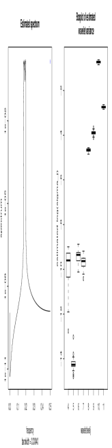
Figure 1: EDA from 26 seconds recording: (left) estimated spectrum and (right) boxplots of estimated wavelet variances on a log-scale for level 4 to 11.

This latter model is interesting in three aspects. First Johnstone and Silverman (1997) show that stationary correlated noise $\tilde{\boldsymbol{\varepsilon}}_{q}$ is well decorrelated by a wavelet transform within and between levels. And for a given level $j$, the nearly white noise process has its own wavelet variance $\sigma_{j}^{2,(q)}$ (Percival, 1995; Serroukh et al., 2000) that can be estimated from the data (Donoho and Johnstone, 1995). The right plot of Figure 1 represents boxplots of such wavelet variances estimated from $31$ disjoint signals of length $N=4096$ for $j=4,\ldots,11$. The left plot of Figure 1 shows an estimated spectrum from 26 seconds of recording: the noise of the captor is a band-pass filtered colored noise process. Second, the data are Gaussianized by the linear wavelet transformation. Third, owing to sparse wavelet representation, the vectors ${\boldsymbol{\beta}}^{(q)}$ are sparse, and the amount of sparsity varies between levels, so the selection of hyperparameters should be level dependent. Hence organizing the coefficients of captor $q$ by levels, model (3) and (4) can be well approximated at a given level $j$ by

$${\boldsymbol{Y}}_{j}^{(q)}={\boldsymbol{\alpha}}_{j}^{(q)}+{\boldsymbol{z}}_{j}^{(q)}\quad{\rm with}\quad{\boldsymbol{Y}}_{j}^{(q)}={\boldsymbol{S}}_{j}^{(q)}/\sigma_{j}^{(q)}\quad{\rm and}\quad{\boldsymbol{\alpha}}_{j}^{(q)}={\boldsymbol{\beta}}_{j}^{(q)}/\sigma_{j}^{(q)},$$ (5)

where ${\boldsymbol{\alpha}}_{j}^{(q)}=(\alpha_{j,1}^{(q)},\ldots,\alpha_{j,N_{j}}^{(q)})$ is a sparse vector and ${\boldsymbol{z}}_{j}^{(q)}\stackrel{{\scriptstyle{\rm i.i.d.}}}{{\sim}}{\rm N}(0,1)$. Importantly, given a dilation $j$ and a translation $n$, then ${\boldsymbol{\alpha}}_{j,n}=(\alpha_{j,n}^{(1)},\ldots,\alpha_{j,n}^{(Q)})$ is either null or, when ${\boldsymbol{\alpha}}_{j,n}\neq{\bf 0}$, then its entries are different. Our goal is to derive an estimator that adapts levelwise to block sparsity.

3 Smooth blockwise iterative thresholding

3.1 Review of block coordinate relaxation

Recent estimators consider the situation where the coefficients are blocked into $J$ groups ${\boldsymbol{\beta}}=({\boldsymbol{\beta}}_{1},\ldots,{\boldsymbol{\beta}}_{J})$ of respective sizes $p_{1},\ldots,p_{J}$ with $\sum_{j=1}^{J}p_{j}=P$. Correspondingly, let $X=[X_{1}\ldots X_{J}]$. For instance, for gravitational wave burst detection, wavelet coefficients are grouped into blocks of size $Q$, the number of captors, and $X_{j}$ is the $Q\times Q$ identity matrix for all $j=1,\ldots,J$.

We recall an optimization technique upon which we elaborate a new estimator in the following section. Suppose for now we want to calculate $\hat{\boldsymbol{\beta}}^{\rm MLE}$ solution to (2) for $\lambda=0$. Block coordinate relaxation (BCR) works as follows: start with any initial guess ${\boldsymbol{\beta}}$, choose a block $j\in\{1,\ldots,J\}$ and update only the $j$th block ${\boldsymbol{\beta}}_{j}$ conditional on the values of the other blocks ${\boldsymbol{\beta}}_{i}$ for all $i\neq j$, that is

$${\boldsymbol{\beta}}_{j}^{\mid{\rm MLE}}={\rm arg}\min_{{\boldsymbol{\beta}}_{j}\in{\cal B}_{j}}-l(\sum_{i\neq j}X_{i}{\boldsymbol{\beta}}_{i}+X_{j}{\boldsymbol{\beta}}_{j};{\bf y}),$$ (6)

and leave the other unchanged to obtain the next iterate

$${\boldsymbol{\beta}}^{(j)}=({\boldsymbol{\beta}}_{1},\ldots,{\boldsymbol{\beta}}_{j-1}, {\boldsymbol{\beta}}_{j}^{\mid{\rm MLE}} ,{\boldsymbol{\beta}}_{j+1},\ldots,{\boldsymbol{\beta}}_{J}).$$ (7)

Note that $j$ is the index of the updated block, but not of the iteration.

Property 1: Assuming that ${\boldsymbol{\beta}}\in{\cal B}$, where ${\cal B}={\cal B}_{1}\times\ldots\times{\cal B}_{J}$ is a product of closed convex sets, that (6) has a unique solution and that the log-likelihood is continuously differentiable, then the algorithm converges to a stationary point (Bertsekas, 1999, Proposition 2.7.1). If the negative log-likelihood is also strictly convex, then the algorithm finds the MLE.

Property 2: After updating ${\boldsymbol{\beta}}$ with ${\boldsymbol{\beta}}^{(j)}$ according to (7), the gradient of the likelihood with respect to the $j$th block is null, that is $\nabla_{{\boldsymbol{\beta}}_{j}}l(X{\boldsymbol{\beta}}^{(j)};{\bf y})={\bf 0}$.

3.2 Smooth blockwise iterative thresholding estimator

The MLE does not achieve variable selection however. To do so, one can test the significance of the $j$th block based on the likelihood and its gradient in the following way. Suppose we are at the MLE where the entire gradient vector is null. The covariates have been $\Sigma$-rescaled for all MLE coefficients to have unit variance as discussed in Section 1. So if after thresholding the $j$th block of the MLE to zero the gradient with respect to the $j$th block remains small (compared to a threshold $\lambda$), then we declare this block not significant. This suggests calculating the likelihood’s block gradient at each BCR iteration:

• at the current iterate ${\boldsymbol{\beta}}^{(j)}$ defined by (7). According to Property 2, the gradient with respect to the $j$th block is null;

• at the current iterate with ${\boldsymbol{\beta}}_{j}^{\mid{\rm MLE}}$ thresholded to ${\bf 0}$, namely at

  $${\boldsymbol{\beta}}^{(j)\rightarrow 0}=({\boldsymbol{\beta}}_{1},\ldots,{\boldsymbol{\beta}}_{j-1}, {\bf 0} ,{\boldsymbol{\beta}}_{j+1},\ldots,{\boldsymbol{\beta}}_{J}).$$ (8)

  The gradient with respect to the $j$th block is $\nabla_{{\boldsymbol{\beta}}_{j}}l(X{\boldsymbol{\beta}}^{(j)\rightarrow 0};{\bf y})$.

A difference larger than a threshold $\lambda$ between the two likelihood’s block gradient norms, that is, $\|\nabla_{{\boldsymbol{\beta}}_{j}}l(X{\boldsymbol{\beta}}^{(j)\rightarrow 0};{\bf y})\|\geq\lambda$, shows that the $j$th block is significant given the value of the other blocks. This leads to the following estimator.

Smooth block iterative thresholding estimator (SBITE) (algorithmic definition). Choose a threshold $\lambda\geq 0$, a shrinkage parameter $\nu\geq 1$ and a smoothness parameter $s\geq 1$. Let $\tilde{\boldsymbol{\beta}}^{*}$ be a root-$N$-consistent estimate of ${\boldsymbol{\beta}}$.

1. Start with any initial value;

2. Choose a block $j$, and calculate ${\boldsymbol{\beta}}_{j}^{\mid{\rm MLE}}$ according to (6) and the gradient $\nabla_{{\boldsymbol{\beta}}_{j}}l(X{\boldsymbol{\beta}}^{(j)\rightarrow 0};{\bf y})$;

3. Update the $j$th block according to

   $${\boldsymbol{\beta}}_{j}^{\rm update}=(1-\frac{\lambda^{\nu}}{\|\tilde{\boldsymbol{\beta}}_{j}^{*}\|^{\nu-1}\|\nabla_{{\boldsymbol{\beta}}_{j}}l(X{\boldsymbol{\beta}}^{(j)\rightarrow 0};{\bf y})\|})^{s}_{+}{\boldsymbol{\beta}}_{j}^{\mid{\rm MLE}};$$ (9)

4. Go back to step 2 until convergence.

The thresholding function (9) is called smooth James-Stein: when $\|\tilde{\boldsymbol{\beta}}_{j}^{*}\|^{\nu-1}$ and $\|\nabla_{{\boldsymbol{\beta}}_{j}}l(X{\boldsymbol{\beta}}^{(j)\rightarrow 0};{\bf y})\|$ are small, thresholding sets the $j$th block to zero. We study the advantage of the smoothness parameter $s$ later. For $s=1$ and certain values of $\nu$, SBITE is linked to existing estimators, as established in the following property.

Property 3 (Gaussian case with a smoothness parameter $s=1$): The SBITE iterations converge at the limit to the estimate of:

1. lasso (Tibshirani, 1996) for $s=\nu=1$ and blocks of size one. Lasso is not an oracle procedure (Fan and Li, 2001b).

2. group lasso (Bakin, 1999; Yuan and Lin, 2006) for $s=\nu=1$, with blocks.

3. adaptive lasso, which is oracle (Zou, 2006), for $s=1$ and $\nu>1$ and blocks of size one. Adaptive lasso is the motivation for including the norm $\|\tilde{\boldsymbol{\beta}}_{j}^{*}\|$ in (9). Hence not only a larger gradient but also a larger root-$N$-consistent estimate of the $j$th block leads to milder shrinkage.

4. waveshrink for $s=1$ and $X$ an orthonormal wavelet matrix: soft-waveshrink for $\nu=1$ and hard-waveshrink when $\nu\rightarrow\infty$.

5. truncated James-Stein for $\nu=2$, $\lambda=\sqrt{P-2}$ and a block of size $P>2$.

6. block thresholding for wavelet smoothing for $s=1$, $\nu=2$, groups of size $L>1$ and $X$ an orthonormal wavelet matrix (Cai, 1999).

For a proof, observe that the SBITE algorithm corresponds to the shooting algorithm (Fu, 1998) for lasso, the BCR algorithm (Sardy et al., 2000) for basis pursuit (Chen et al., 1999) and to the iterative algorithm of Yuan and Lin (2006) to minimize penalized least squares problems of the form

$$\min_{{\boldsymbol{\beta}}}\frac{1}{2}\|{\bf Y}-X{\boldsymbol{\beta}}\|_{2}^{2}+\lambda\sum_{j=1}^{J}\frac{1}{\|\tilde{\boldsymbol{\beta}}_{j}^{*}\|^{\nu-1}}\|{\boldsymbol{\beta}}_{j}\|_{2}.$$ (10)

Note that the last three estimators above (4, 5, 6) converge after one iteration, and (10) can also be solved by another class of iterative algorithms developed for inverse problems (Daubechies et al., 2004).

Hence SBITE provides a new interpretation of lasso as a sequence of tests based on the block gradient of the likelihood evaluated at successive null hypothesis $H_{0}:{\boldsymbol{\beta}}_{j}={\bf 0}$ given the values of the other coefficients, until an equilibrium is reached. A legitimate question addressed in the following section is whether such an equilibrium can be reached at a unique point. If so, SBITE is defined uniquely.

3.3 Uniqueness

Lasso ($s=1$) does not necessarily define a unique estimate if the kernel of the regression matrix $X$ is not the ${\bf 0}$ singleton (Sardy, 2009). On the contrary SBITE is uniquely defined under a milder condition when $s>1$, as stated in Theorem 1 below. We first give its fixed point definition.

Smooth block iterative thresholding estimator (SBITE) (fixed point definition). Choose a threshold $\lambda\geq 0$, a shrinkage parameter $\nu\geq 1$ and a smoothness parameter $s\geq 1$. Let $\tilde{\boldsymbol{\beta}}^{*}$ be a root-$N$-consistent estimate of ${\boldsymbol{\beta}}$. SBITE is a fixed point to the SBITE algorithm, which is the solution to the set of $P$ nonlinear equations

$${\boldsymbol{\beta}}_{j}=(1-\frac{\lambda^{\nu}}{\|\tilde{\boldsymbol{\beta}}_{j}^{*}\|^{\nu-1}\|\nabla_{{\boldsymbol{\beta}}_{j}}l(X{\boldsymbol{\beta}}^{(j)\rightarrow 0};{\bf y})\|})^{s}_{+}{\boldsymbol{\beta}}_{j}^{\mid{\rm MLE}},\quad j=1,\ldots,J,$$ (11)

where ${\boldsymbol{\beta}}_{j}^{\mid{\rm MLE}}$ is defined by (6), and each ${\boldsymbol{\beta}}_{j}$ is a vector of length $p_{j}$ with $P=\sum_{j=1}^{J}p_{j}$.

Despite being highly non-linear and employing a non-convex thresholding function, these equations define SBITE uniquely in the Gaussian case when $s>1$.

Theorem 1: For the Gaussian likelihood, the solution to (11) with smoothness parameter $s>1$ is uniquely defined for all matrices $X=[X_{1}\ldots X_{J}]$ such that $X_{j}^{\rm T}X_{j}$ are positive definite matrices for all $j=1,\ldots,J$. It is moreover continuously differentiable with respect to the data.

Note that the condition is milder than $X^{\rm T}X$ being positive definite; for unit block size, its means that each column of $X$ must be different from the zero-vector. Convergence of the SBITE algorithm is proved when $s=1$ for the Gaussian likelihood (Fu, 1998; Sardy et al., 2000) and for more general likelihoods (Sardy and Tseng, 2004). Convergence to the unique fixed point has always been observed when $s>1$, but remains to be proved.

3.4 Equivalent degrees of freedom

SBITE is governed by two regularization parameters $\lambda$ and $\nu$, and a smoothness parameter $s$. For $s=1$ and for the Gaussian linear model with mean ${\boldsymbol{\mu}}=X{\boldsymbol{\alpha}}$ and $P$ variables grouped into blocks of unit size, Zou (2006) selects the two regularization parameters $\lambda$ and $\nu$ of adaptive lasso by cross-validation, a rule known for its high computational cost and instability. This section derives instead the Stein unbiased risk estimate for any combination of the three parameters $(\lambda,\nu,s)$.

Stein (1981) showed that for an estimator of the form $\hat{\boldsymbol{\mu}}=g({\bf Y})+{\bf Y}$ and unit variance, then the quadratic risk can be estimated unbiasedly if $g$ is almost differentiable. For SBITE with blocks of unit size, we have $g({\bf Y};\lambda,\nu,s)=\bar{\bf Y}{\bf 1}+X\hat{\boldsymbol{\beta}}_{\lambda,\nu;s}({\bf Y})-{\bf Y}$, where $\hat{\boldsymbol{\beta}}_{\lambda,\nu;s}({\bf Y})$ is the solution to (11) for Gaussian likelihood. SBITE is almost differentiable for $s=1$ and differentiable for $s>1$, so the Stein unbiased risk estimate (SURE) for SBITE is

$${\rm SURE}(\lambda,\nu;s)={\rm RSS}(\hat{\boldsymbol{\mu}}_{\lambda,\nu,s})+N+2\sum_{n=1}^{N}\partial g_{n}({\bf Y};\lambda,\nu,s)/\partial Y_{n},$$ (12)

where the last term is the so-called equivalent degrees-of-freedom. SURE involves the partial derivatives $\partial g_{n}({\bf Y};\lambda,\nu,s)/\partial Y_{n}=1/N+{\bf x}_{n}^{\rm row}\cdot\nabla_{n}\hat{\boldsymbol{\beta}}_{\lambda,\nu,s}({\bf Y})-1$, for $n=1,\ldots,N$, where $\nabla_{n}\hat{\boldsymbol{\beta}}_{\lambda,\nu,s}({\bf Y})$ are the derivatives of $\hat{\boldsymbol{\beta}}_{\lambda,\nu,s}({\bf Y})$ with respect to $Y_{n}$, and ${\bf x}_{n}^{\rm row}$ is the $n$th row of $X$. The following theorem states that $\nabla_{n}\hat{\boldsymbol{\beta}}_{\lambda,\nu,s}({\bf Y})$ is explicitly defined as solution to a full rank system of linear equations when $s>1$. Hence the risk of SBITE can be estimated unbiasedly for all regression matrix.

Theorem 2: For a given pair $\lambda>0$ and $\nu\geq 1$ and for a linear estimate $\tilde{\boldsymbol{\beta}}^{*}=A{\bf Y}$ (e.g., least squares or ridge regression) where the entries of $A$ are noted $a_{pn}$, the gradient of the SBITE estimate $\hat{\boldsymbol{\beta}}_{\lambda,\nu,s}({\bf Y})$ with respect to $Y_{n}$ is the solution to a system of linear equations (30) that is full rank when $s>1$, regardless of the existence of a kernel for $X$, for $n=1,\ldots,N$.

Interestingly also from Theorem 2, letting the smoothness parameter $s$ tend to one leads to the equivalent degrees of freedom of adaptive lasso; if moreover $\nu=1$, then the solution to (30) is ${\bf h}_{n}^{\bar{\cal I}_{0}}=((X^{\bar{\cal I}_{0}})^{\rm T}X^{\bar{\cal I}_{0}})^{-1}({\bf x}_{n}^{\rm row})^{\rm T}$. Hence, we see that

$$\sum_{n=1}^{N}\partial g_{n}({\bf Y};\lambda,\nu,s)/\partial Y_{n} = 1+\sum_{n=1}^{N}{\bf x}_{n}^{\rm row}\cdot((X^{\bar{\cal I}_{0}})^{\rm T}X^{\bar{\cal I}_{0}})^{-1}({\bf x}_{n}^{\rm row})^{\rm T}-N$$

$$= 1+{\rm trace}(((X^{\bar{\cal I}_{0}})^{\rm T}X^{\bar{\cal I}_{0}})^{-1}((X^{\bar{\cal I}_{0}})^{\rm T}X^{\bar{\cal I}_{0}}))-N$$

$$= 1+|\bar{\cal I}_{0}|-N,$$

where $|\bar{\cal I}_{0}|$ is lasso’s degrees of freedom previously found by Zou et al. (2007).

The smoothness parameter should not be considered as a third regularization parameter like $\lambda$ and $\nu$, but more like a device to bring smoothness to the estimator and combat the increasing erraticity of the two-dimensional SURE function as $\nu$ grows. Section 4.1 quantifies SURE’s erraticity tempered with the smoothness parameter $s$. The smoothness parameter should not be too large however, since it contradicts the goal of a large $\nu$ to approach hard thresholding, and since the constant of the oracle inequality (21) of Theorem 4 increases with $s$. A good trade-off is for instance $s(\nu)=2\log\nu+1$ (see Theorem 3 below). Figure 2 illustrates the gain in smoothness by calculating SURE for the prostate cancer data with $P=8$ covariates (Tibshirani, 1996), and by comparing the smoothness of the estimated risk either with adaptive lasso (left) or with its smooth extension (right). Both risk estimates are unbiased, but the second is less erratic thanks to $s>1$.

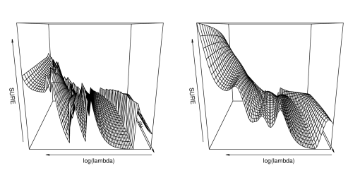
Figure 2: Prostate cancer data: Stein unbiased risk estimate as a function of $\lambda$ and $\nu$ for adaptive lasso (left, $s=1$) and smooth adaptive lasso (right, $s=2\log\nu+1$).

We have assumed unit variance. In practice, one can either estimate the variance and rescale responses to have approximate unit variance, or, in the spirit of generalized cross validation (Golub et al., 1979), one can use generalized SURE

$${\rm GSURE}(\lambda,\nu;s)=\frac{{\rm RSS}(\hat{\boldsymbol{\mu}}_{\lambda,\nu;s})/N}{(1-\frac{1}{N}\sum_{n=1}^{N}\partial g_{n}({\bf Y};\lambda,\nu,s)/\partial Y_{n})^{2}}.$$ (13)

To minimize SURE or GSURE over $(\lambda,\nu)$ for $s=2\log\nu+1$, our strategy consists in minimizing it first for $s=1$ (i.e., adaptive lasso) which can be done efficiently on a fine grid thanks to lars (Efron et al., 2004). This provides a neighborhood for $\lambda$, namely $[\hat{\lambda}^{(s=1)}/10,10\hat{\lambda}^{(s=1)}]$, over which we then minimize SURE on a more local grid for smooth adaptive lasso ($s>1$) calculated with the SBITE algorithm. This strategy provides a good and efficient selection of the pair of hyperparameters $(\lambda,\nu)$, as demonstrated by Monte-Carlo below.

3.5 Monte-Carlo simulation

We replicate the Monte-Carlo simulation of Zou (2006) with $P=8$ covariates with corresponding coefficients either sparse ${\boldsymbol{\alpha}}=(3,1.5,0,0,2,0,0,0)$ for Model 1 with $N\in\{20,60\}$, or not sparse ${\boldsymbol{\alpha}}=(.85,.85,.85,.85,.85,.85,.85,.85)$ for Model 2 with $N\in\{40,80\}$. The covariates $\tilde{\bf x}_{n}$ are i.i.d. Gaussian vectors with pairwise correlation between $\tilde{x}_{n,i}$ and $\tilde{x}_{n,j}$ given by ${\rm cor}(i,j)=(.5)^{|i-j|}$. The noise is Gaussian with standard error $\sigma\in\{1,3,6\}$. Like Zou (2006), we consider the relative prediction error ${\rm RPE}={\rm E}[\tilde{\bf x}_{\rm test}^{\rm T}\{\hat{\boldsymbol{\alpha}}([\tilde{X},{\bf Y}]_{\rm training})-{\boldsymbol{\alpha}}\}]/\sigma^{2}$, where the expectation is taken over training and test sets, and response. Note that we exactly calculate RPE given the training set by using knowledge of the distribution of the covariates (Zou relies on 10,000 test observations instead). This predictive measure is reported in Table 1 to compare lasso, adaptive lasso and smooth adaptive lasso. To compare estimators fairly, we consider the same selection rule for all, here two-fold cross-validation. Since the estimators are used on the same 100 training sets, then the numbers we see in the tables reveal significant differences, even though marginal standard errors are large. We observe that SBITE improves significantly over lasso and adaptive lasso when the underlying model is sparse and the noise is small; the estimation is slightly worse for the non-sparse model.

Table 1: Zou’s Monte-Carlo simulation with 100 training sets: median RPE using two-fold cross-validation to select the hyperparameter(s).

	$\sigma=1$		$\sigma=3$		$\sigma=6$
Model 1	$N=20$	$N=60$	$N=20$	$N=60$	$N=20$	$N=60$
lasso	$0.367_{(0.048)}$	$0.089_{(0.009)}$	$0.419_{(0.069)}$	$0.089_{(0.008)}$	$0.369_{(0.021)}$	$0.096_{(0.010)}$
adaptive lasso	$0.360_{(0.051)}$	$0.052_{(0.009)}$	$0.435_{(0.057)}$	$0.085_{(0.009)}$	$0.308_{(0.021)}$	$0.097_{(0.011)}$
SBITE	$0.328_{(0.046)}$	$0.054_{(0.009)}$	$0.424_{(0.056)}$	$0.085_{(0.009)}$	$0.330_{(0.020)}$	$0.098_{(0.010)}$
Model 2	$N=40$	$N=80$	$N=40$	$N=80$	$N=40$	$N=80$
lasso	$0.238_{(0.014)}$	$0.104_{(0.005)}$	$0.231_{(0.020)}$	$0.108_{(0.005)}$	$0.163_{(0.010)}$	$0.087_{(0.005)}$
adaptive lasso	$0.238_{(0.015)}$	$0.104_{(0.005)}$	$0.233_{(0.021)}$	$0.108_{(0.005)}$	$0.181_{(0.010)}$	$0.091_{(0.005)}$
SBITE	$0.238_{(0.015)}$	$0.104_{(0.005)}$	$0.240_{(0.021)}$	$0.109_{(0.005)}$	$0.172_{(0.010)}$	$0.090_{(0.005)}$

We also consider SURE as a selection rule for lasso and its smooth adaptive version SBITE, that we compare based on their relative prediction error conditional on the covariates of the training set, namely ${\rm RPE}\mid\tilde{X}=\sum_{n=1}^{N}{\rm E}[\tilde{\bf x}_{{\rm training},n}^{\rm T}\{\hat{\boldsymbol{\alpha}}([\tilde{X},{\bf Y}]_{\rm training})-{\boldsymbol{\alpha}}\}]/\sigma^{2}$, where the expectation is taken over the response only. Although less useful in practice unless prediction is sought at the same locations as the training set, this measure helps quantify the improvement of using smooth James-Stein thresholding. Table 2 reports the results, which shows a systematic gain of SBITE over adaptive lasso. Lasso is often better for the non-sparse model.

Table 2: Zou’s Monte-Carlo simulation with 100 training sets: median RPE $\mid X$ at the training covariates $X$ using SURE to select the hyperparameter(s).

	$\sigma=1$		$\sigma=3$		$\sigma=6$
Model 1	$N=20$	$N=60$	$N=20$	$N=60$	$N=20$	$N=60$
lasso	$0.264_{(0.021)}$	$0.082_{(0.008)}$	$0.258_{(0.020)}$	$0.082_{(0.008)}$	$0.219_{(0.017)}$	$0.082_{(0.007)}$
adaptive lasso	$0.231_{(0.023)}$	$0.075_{(0.008)}$	$0.280_{(0.023)}$	$0.090_{(0.008)}$	$0.289_{(0.019)}$	$0.096_{(0.007)}$
SBITE	$0.228_{(0.023)}$	$0.065_{(0.008)}$	$0.279_{(0.025)}$	$0.084_{(0.008)}$	$0.255_{(0.019)}$	$0.097_{(0.007)}$
Model 2	$N=40$	$N=80$	$N=40$	$N=80$	$N=40$	$N=80$
lasso	$0.187_{(0.010)}$	$0.092_{(0.004)}$	$0.187_{(0.010)}$	$0.090_{(0.004)}$	$0.137_{(0.008)}$	$0.075_{(0.003)}$
adaptive lasso	$0.191_{(0.011)}$	$0.092_{(0.004)}$	$0.237_{(0.013)}$	$0.127_{(0.006)}$	$0.172_{(0.009)}$	$0.105_{(0.004)}$
SBITE	$0.191_{(0.011)}$	$0.092_{(0.004)}$	$0.219_{(0.013)}$	$0.113_{(0.006)}$	$0.164_{(0.008)}$	$0.099_{(0.004)}$

Finally Table 3 reports the number $C$ of selected nonzero components and the number $I$ of zero components incorrectly selected. We observe that the selection is correct when the noise is small ($\sigma=1$) with SBITE and adaptive lasso using SURE, but that false detection grows with noise.

Table 3: Median number of Selected Variables for Model 1 with $n=60$

	$\sigma=1$			$\sigma=3$
	C	I		C	I
Truth	3	0		3	0
Lasso†	3	2		3	2
Adaptive lasso†	3	1		3	1
SCAD†	3	0		3	1
Garotte†	3	1		3	1.5
Adaptive lasso SURE	3	0		4	1
SBITE SURE	3	0		5	2

^† Results taken from the Monte-Carlo simulation of Zou (2006).

4 Block canonical regression

We consider block canonical regression, that is when the regression matrix is the identity and the coefficients are organized in blocks of size $Q$, namely,

$${\bf Y}_{n}={\boldsymbol{\alpha}}_{n}+{\boldsymbol{\epsilon}}_{n}\quad{\rm with}\quad{\bf Y}_{n}=\left(\begin{array}[]{c}Y_{n}^{(1)}\\ \vdots\\ Y_{n}^{(Q)}\end{array}\right),\ {\boldsymbol{\alpha}}_{n}=\left(\begin{array}[]{c}\alpha_{n}^{(1)}\\ \vdots\\ \alpha_{n}^{(Q)}\end{array}\right)\ {\rm and}\ {\boldsymbol{\epsilon}}_{n}=\left(\begin{array}[]{c}\epsilon_{n}^{(1)}\\ \vdots\\ \epsilon_{n}^{(Q)}\end{array}\right)$$ (14)

for $n=1,\ldots,N$, where the noise is i.i.d. Gaussian (independent between and within sequences). If the standard deviation is not known, then Donoho and Johnstone (1994) proposed an efficient estimate based on the median absolute deviation; another possibility is to use generalized SURE (13). This setting applies to the gravitational wave bursts detection problem (5) of Section 2 with $Q$ captors. Since $X$ is the identity, rescaling has no impact, that is $\tilde{X}=X$ and $\beta=\alpha$.

Block sparsity assumes most blocks ${\boldsymbol{\alpha}}_{n}$ are the ${\bf 0}$-vector. SBITE (11) achieves block sparsity and has the closed form expression

$$(\hat{\boldsymbol{\alpha}}_{n})_{\lambda,\nu;s} = (1-\frac{\lambda^{\nu}}{\|{\bf Y}_{n}\|_{2}^{\nu}})_{+}^{s}{\bf Y}_{n},\quad n=1,\ldots,N.$$ (15)

in this canonical setting.

4.1 Total variation of SURE

The Stein unbiased risk estimate also has the closed form expression ${\rm SURE}(\lambda,\nu,s)=\sum_{n=1}^{N}\hat{\rho}_{n}((\lambda,\nu,s),{\boldsymbol{\alpha}}_{n})$ with

$$\hat{\rho}_{n}((\lambda,\nu,s),{\boldsymbol{\alpha}}_{n})=\{1-(1-\frac{\lambda^{\nu}}{\|{\bf Y}_{n}\|_{2}^{\nu}})_{+}^{s}\}^{2}\|{\bf Y}_{n}\|_{2}^{2}-Q+2\sum_{q=1}^{Q}\frac{\partial(\hat{\boldsymbol{\alpha}}_{n})_{\lambda,\nu;s}}{\partial Y_{n}^{(q)}},$$

where

$$\frac{\partial(\hat{\boldsymbol{\alpha}}_{n})_{\lambda,\nu;s}}{\partial Y_{n}^{(q)}}=\left\{\begin{array}[]{ll}0&{\rm if}\ \|{\bf Y}_{n}\|_{2}<\lambda\\ (1-\frac{\lambda^{\nu}}{\|{\bf Y}_{n}\|_{2}^{\nu}})^{s-1}(\nu s\lambda^{\nu}\frac{(Y_{n}^{(q)})^{2}}{\|{\bf Y}_{n}\|_{2}^{\nu+2}}+1-\frac{\lambda^{\nu}}{\|{\bf Y}_{n}\|_{2}^{\nu}})&{\rm if}\ \|{\bf Y}_{n}\|_{2}\geq\lambda\end{array}\right..$$ (16)

For thresholding functions employing no smoothness, that is $s=1$ here, SURE has $N$ discontinuity points as a function of $\lambda$ for a fixed $\nu$. Indeed (16) is discontinuous at $\lambda=\|{\bf Y}_{n}\|_{2}$ for all $n=1,\ldots,N$ when $s=1$, and the size of each jump is equal to $2\nu$. We had already observed on the left graph of Figure 2 that the larger $\nu$ the more erratic the SURE surface for the prostate cancer data when $s=1$. There are two negative consequences for the selection of $\lambda$ and $\nu$. First the SURE two-dimensional surface will have minima that will be difficult to localize from an optimization point-of-view. Second, the location of the global minima will be sensitive, in particular with large $\nu$, to changes in the data ${\bf Y}_{n}$.

Donoho and Johnstone (1995) studied the asymptotic properties of selecting $\lambda$ by minimizing SURE for $\nu=s=1$. To show their SureShrink estimator is optimally smoothness adaptive, a key ingredient is the deviation of SURE around its mean when $\nu=1$.

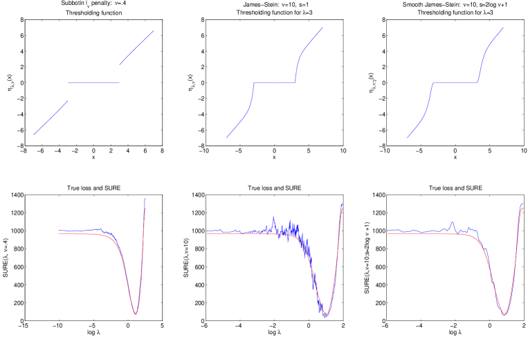
Figure 3: Thresholding functions and corresponding SURE for $Q=1$ and $\nu=10$ on simulated data of length $N=1000$. Left: Subbotin $\ell_{\nu}$ penalized least squares; Middle: James-Stein ($s=1$); Right: smooth James-Stein ($s=2\log\nu+1$). Top: thresholding functions with parameters chosen to approximate hard thresholding. The left one is discontinuous at the threshold, but with a small slope at the threshold; the middle one has a discontinuous derivative at the threshold; and the right one has a smooth change of derivative at the threshold. Bottom: corresponding Stein unbiased risk estimate (least smooth curve) and true loss (smoothest curve).

Theorem 3 below shows that the total variation of SURE grows when $\nu$ increases, and that employing smooth James-Stein thresholding with a smoothness parameter larger than one tempers this erratic effect by removing the jumps and decreasing the erraticity of SURE. Figure 3 illustrates the advantage of increasing $s$ when $\nu$ gets large on simulated data. We observe that while the two thresholding functions for $s=1$ and $s>1$ only differ slightly, the latter is smoother near the threshold value and the corresponding SURE curve is less wiggly around the true loss. Section 4.5 reports results of a Monte-Carlo simulation that quantifies the improvement in mean squared error obtained by adding smoothness.

A measure of erraticity of SURE that is defined not only for $s>1$ but also for $s=1$ is its total variation as a function of $\lambda$. The total variation of a function $f$ in the space of functions of bounded variation (that is, not necessarily continuous) is ${\rm TV}(f)=\sup\sum_{j}|f(\lambda_{j+1})-f(\lambda_{j})|$, where the supremum is taken over all possible partitions $[\lambda_{j},\lambda_{j+1}]$, $j=1,\dots,M$, of the domain of $f$. (If $f$ is moreover absolutely continuous, then TV reduces to the more conventional smoothness measure ${\rm TV}(f)=\int_{\Lambda}|f^{\prime}(\lambda)|d\lambda$.) The following theorem quantifies the erraticity of SURE and shows the tempering effect of the smoothness parameter $s$.

Theorem 3: Consider ${\rm SURE}(\lambda;\nu,s)=\sum_{n=1}^{N}\hat{\rho}_{n}((\lambda;\nu,s),{\boldsymbol{\alpha}}_{n})$ as a function of $\lambda$ for $Q=1$. Its total variation for a given $\nu\geq 1$ satisfies

$${\rm TV}^{(s=1)}({\rm SURE})=\sum_{n=1}^{N}{\rm TV}^{(s=1)}(\hat{\rho}_{n})>\sum_{n=1}^{N}{\rm TV}^{(s>1)}(\hat{\rho}_{n})\geq{\rm TV}^{(s>1)}({\rm SURE}).$$

Moreover erraticity increases less with $s>1$ when $\nu$ or $|Y_{n}|$ grows since $\frac{\partial}{\partial\nu}{\rm TV}^{(s>1)}(\hat{\rho}_{n})\leq\frac{\partial}{\partial\nu}{\rm TV}^{(s=1)}(\hat{\rho}_{n})$ and $\frac{\partial}{\partial Y_{n}}{\rm TV}^{(s>1)}(\hat{\rho}_{n})\leq\frac{\partial}{\partial Y_{n}}{\rm TV}^{(s=1)}(\hat{\rho}_{n})$ for ${Y_{n}\geq 0}$. In particular when $Y_{n}\rightarrow 0$ and for $\nu$ large, then $\frac{\partial}{\partial\nu}{\rm TV}^{(s>1)}(\hat{\rho}_{n})\rightarrow 4(1-1/s)^{s-1}\geq 4\exp(-1)$ for $s$ fixed. Letting $s$ grow slowly with $\nu$, for instance $s(\nu)=2\log\nu+1$, then the lower bound $4\exp(-1)$ is reached to lower erraticity most.

4.2 Universal threshold and information criterion

To derive a universal threshold (Donoho and Johnstone, 1994) and an information criterion for SBITE, we approximate below the distribution of the smallest threshold $\lambda_{{\cal Y}}$ that, for a sample ${\cal Y}=({\bf Y}_{1},\ldots,{\bf Y}_{N})$ of size $N$, sets to zero all $N$ blocks of length $Q$ when the true underlying model is made of zero vectors. Controlling the maximum of $\lambda_{{\cal Y}}$ then leads to a finite sample $\tilde{\lambda}_{N,Q}$ and asymptotic $\lambda_{N,Q}$ universal thresholds, and a prior distribution $\pi_{\lambda}$ for $\lambda$.

Assuming ${\bf Y}_{n}\stackrel{{\scriptstyle{\rm i.i.d.}}}{{\sim}}{\rm N}_{Q}({\bf 0},I_{Q})$ for $n=1,\ldots,N$, we seek the smallest threshold $\lambda_{N,Q}$ such that SBITE estimates the right model with a probability tending to one:

$${\rm P}((\hat{\boldsymbol{\alpha}}_{1})_{\lambda_{N,Q},\nu;s}={\bf 0},\ldots,(\hat{\boldsymbol{\alpha}}_{N})_{\lambda_{N,Q},\nu;s}={\bf 0})={\rm P}(\max_{n=1,\ldots,N}\|{\bf Y}_{n}\|_{2}^{2}\leq\lambda_{N,Q}^{2})\stackrel{{\scriptstyle N\rightarrow\infty}}{{\longrightarrow}}1.$$ (17)

The distribution of $M_{N}=\max_{n=1}^{N}\|{\bf Y}_{n}\|_{2}^{2}$, where $\|{\bf Y}_{n}\|_{2}^{2}\stackrel{{\scriptstyle\rm i.i.d.}}{{\sim}}\chi_{Q}^{2}=\Gamma(Q/2,1/2)$, is degenerate. Extreme value theory provides proper rescaling of $M_{N}$ for $c_{N}^{-1}(M_{N}-d_{N}(Q))\longrightarrow_{d}G_{0}(x)$, where $G_{0}(x)=\exp(-\exp(-x))$ is the Gumbel distribution, $c_{N}=2$ and $d_{N}(Q)$ is the root in $\xi$ to

$$\log N-\log\Gamma(Q/2)=(1-Q/2)\log(\xi/2)+\xi/2.$$ (18)

The normalizing constant $d_{N}(Q)=2(\log N+(Q/2-1)\log\log N-\log\Gamma(Q/2))$ given by Embrechts et al. (1997, p.156) for the Gamma distribution is the asymptotic root of (18), which provides a good Gumbel approximation when $N$ is large compared to $\Gamma(Q/2)$. In that case we define the asymptotic universal threshold $\lambda_{N,Q}=\sqrt{2(\log N+(Q/2)\log\log N-\log\Gamma(Q/2))}$, for which (17) is satisfied since

$${\rm P}(\max_{n=1,\ldots,N}\|{\bf Y}_{n}\|_{2}^{2}\leq\lambda_{N,Q}^{2})\stackrel{{\scriptstyle\cdot}}{{=}}G_{0}(\log\log N)\approx 1-1/\log N\stackrel{{\scriptstyle N\rightarrow\infty}}{{\longrightarrow}}1.$$ (19)

Note that we get back the standard universal threshold $\sqrt{2\log N}$ up to a small term for $Q=1$, and the universal threshold of Sardy (2000) for denoising complex-valued signals for $Q=2$. When $Q$ gets large however, the proposed normalizing constant $d_{N}(Q)$ is too far from the exact root to provide a useful approximation, so we find the root $d_{N}(Q)$ of (18) numerically. The finite sample universal threshold is then defined as

$$\tilde{\lambda}_{N,Q}=\sqrt{d_{N}(Q)+c_{N}\log\log N}\quad\mbox{ with }\quad d_{N}(Q)\mbox{ root of }(\ref{eq:rootdN})$$ (20)

to have the same rate of convergence for all $Q$ with $\tilde{\lambda}_{N,Q}$ in place $\lambda_{N,Q}$ in (19).

More than a bound the asymptotic Gumbel pivot for $M_{N}$ leads to a prior distribution $F_{\lambda}(\lambda)=G_{0}((\lambda^{2}-d_{N}(Q))/2)$ of the threshold $\lambda$ to reconstruct true zero vectors from noisy measurements. When $s=1$, Bayes theorem provides the joint posterior distribution of the coefficients and the hyperparameters. Taking its negative logarithm leads to the following information criterion in the spirit of the sparsity $\ell_{\nu}$ information criterion SL_νIC (Sardy, 2009).

Definition. Suppose model (14) or model (3.1) of Cai (1999) holds. The sparsity weighted $\ell_{2}$ information criterion for the estimation of $({\boldsymbol{\alpha}}_{1},\ldots,{\boldsymbol{\alpha}}_{N})$ and the selection of $(\lambda,\nu)$ with SBITE (15) for $s=1$ is defined as

$${\rm SL}_{2}^{w}{\rm IC}({\boldsymbol{\alpha}}_{1},\ldots,{\boldsymbol{\alpha}}_{N},\lambda,\nu) = \frac{1}{2}\sum_{n=1}^{N}\|{\bf Y}_{n}-{\boldsymbol{\alpha}}_{n}\|_{2}^{2}+\lambda^{\nu}\sum_{n=1}^{N}\frac{1}{\|{\bf Y}_{n}\|_{2}^{\nu-1}}\|{\boldsymbol{\alpha}}_{n}\|_{2}$$

$$-N\log(\frac{\Gamma(Q/2)}{2\pi^{Q/2}\Gamma(Q)})+Q(\nu-1)\sum_{n=1}^{N}\log\|{\bf Y}_{n}\|_{2}$$

$$-QN\nu\log\lambda-\log\pi_{\lambda}(\lambda;\tau_{N,Q})-\log\pi_{\nu}(\nu),$$

where $\pi_{\nu}$ is a prior for $\nu$ that we choose Uniform on $[1,\infty)$, $\pi(\lambda;\tau)=F^{\prime}(\lambda;\tau)$ with $F_{\lambda}(\lambda;\tau)=G_{0}((\lambda^{2}/\tau^{2}-d_{N}(Q))/2)$ and $\tau$ is calibrated to $\tau_{N,Q}^{2}=\tilde{\lambda}_{N,Q}^{2}/(QN\nu+1)$ to match the asymptotic model consistency when ${\boldsymbol{\alpha}}_{n}={\bf 0}$ for $n=1,\ldots,N$.

In practice, one minimizes SL${}_{2}^{w}$IC like AIC or BIC to both select the hyperparameters $(\lambda,\nu)$ and estimate the sequences ${\boldsymbol{\alpha}}_{n}$, $n=1,\ldots,N$. The information criterion could also be derived for $s>1$ if we knew the definition of SBITE as a penalized least squares, which is an open problem.

4.3 Oracle inequality

Candès (2005) provides an interesting review on oracle inequalities. Here we derive an oracle inequality for SBITE employing smooth James-Stein thresholding when the block size $Q\geq 2$ is fixed. Cai (1999) derived an oracle inequality for block sizes increasing with the sample size. The $\ell_{2}$ risk for model (14) is ${\rm R}(\hat{\boldsymbol{\alpha}},{\boldsymbol{\alpha}})=\sum_{n=1}^{N}\rho_{n}({\boldsymbol{\alpha}}_{n})=\sum_{n=1}^{N}{\rm E}\|\hat{\boldsymbol{\alpha}}_{n}-{\boldsymbol{\alpha}}_{n}\|_{2}^{2}$. Following Donoho and Johnstone (1994), the oracle predictive performance of the block diagonal projection estimator $\hat{\boldsymbol{\alpha}}_{n}=\delta_{n}{\bf Y}_{n}$, where $\delta_{n}\in\{0,1\}$ is

$$\rho_{n}(\delta_{n},{\boldsymbol{\alpha}}_{n})=\left\{\begin{array}[]{ll}\|{\boldsymbol{\alpha}}_{n}\|_{2}^{2},&{\rm if}\ \delta_{n}=0,\\ Q,&{\rm if}\ \delta_{n}=1.\end{array}\right.$$

Hence the oracle hyperparameters are $\delta_{n}^{*}=1_{\{\|{\boldsymbol{\alpha}}_{n}\|_{2}^{2}>Q\}}$ for $n=1,\ldots,N$, and the corresponding oracle overall risk is ${\rm R}^{*}({\boldsymbol{\delta}},{\boldsymbol{\alpha}})=\sum_{n=1}^{N}\min(\|{\boldsymbol{\alpha}}_{n}\|^{2},Q)$. The following theorem extends the oracle inequality obtained by Donoho and Johnstone (1994) and Zou (2006) for $Q=s=1$ to block thresholding with $Q\geq 2$ and $s>1$.

Theorem 4: For any fixed $Q\geq 2$, there exists a sample size $N_{0}$ such that, for all $N\geq N_{0}$ and with the universal threshold $\tilde{\lambda}_{N,Q}$ defined in (20), then SBITE defined by (15) for $\nu\geq 1$ and $s\geq 1$ achieves the oracle inequality

$${\rm R}(\hat{\alpha}^{{\rm SBITE}}_{\tilde{\lambda}_{N,Q},\nu;s},{\boldsymbol{\alpha}})\leq(Q+1+2\nu s+c_{\nu,s,Q}\lambda_{N,Q}^{2})(Q+{\rm R}^{*}({\boldsymbol{\delta}},{\boldsymbol{\alpha}})),$$ (21)

where $c_{\nu,s,Q}=\max(1+\frac{\nu s}{Q},s^{2})$ and $\lambda_{N,Q}^{2}=2\log N+Q\log\log N-2\log\Gamma(Q/2)$.

This result shows we can mimic the overall oracle risk achieved with $N$ oracle hyperparameters within a factor of essentially $\lambda_{N,Q}^{2}$ with the single hyperparameter $\tilde{\lambda}_{N,Q}$. The smallest sample size $N_{0}$ for which the inequality holds is quite small in practice; more work is needed to get a tight expression. Note that for $s=1$, the inequality differs from Zou (2006) which had the $\nu$-term in the denominator (this seems to be due to an error in $d\hat{\mu}_{i}^{*}(\lambda)/dy_{i}$ right above (A.13) p. 1427). This result shows that increasing $\nu$ or $s$ increases the oracle inequality constant. But this does not prevent the estimator with $\nu>1$ to be oracle (Zou, 2006), which is not true for lasso with $\nu=1$. Likewise using a larger $s$ improves predictive performance in practice although the oracle inequality constant increases.

4.4 Application to wave burst detection and estimation

We employ SBITE blockwise and levelwise to $Q=3$ concomitant time series of length $T=2^{14}$ (about 3.27 seconds of recording) to detect gravitational wave bursts, as described in Section 2.

Figure 4: A wave burst injection at time $t=1500$ added on three real captors noise (columnwise). Top: Time series of length $T=2^{14}$. Middle: SBITE employing SURE levelwise and blockwise. Bottom: univariate smoothing per captor levelwise.

Taking $J=4$ in the wavelet expansion (4), SBITE has a total of $22$ hyperparameters to select (11 levels with two hyperparameters each). Data are pure electronic noise, so we add three proportional so-called “injections” at time $t=1500$, to mimic a wave burst.

Figure 4 shows the data (first line) for each captor (columnwise), the SBIT estimate (second line) and estimates employing a univariate smoothing per captor (third line). We observe that, as opposed to univariate smoothing, blockwise smoothing detects the injection and has no false detection except right before time $t=10^{\prime}000$. Figure 5 zooms around the injections that are three times larger on the second captor, and five times smaller on the third captor. We see that blockwise estimation of the injections is better than coordinatewise.

Figure 5: Zooming on the “injection” represented by the dotted line (the $y$-scales differs between captors). The estimates are plotted with a continuous line: blockwise smoothing (first line), and a univariate smoothing per captor (second line).

4.5 Monte-Carlo simulation

We reproduce the Monte-Carlo simulation of Johnstone and Silverman (2004) for $Q=1$ captor to estimate a sparse sequence of length $N=1000$ and of varying degrees of sparsity, as measured by the number of nonzero terms taken in $\{5,50,500\}$ and by the value of the nonzero terms $\mu$ taken in $\{3,4,5,7\}$. Table 4 reports estimated risks of four estimators: SBITE with ($s>1$) and without ($s=1$) smoothness, Subbotin $\ell_{\nu}$ penalized likelihood (Sardy, 2009) and EBayesThresh (Johnstone and Silverman, 2004). The results clearly show the superiority of SBITE with SURE thanks to more smoothness. In case of extreme sparsity, only SBITE using the SL${}_{2}^{w}$IC information criterion and EBayesThresh perform better; this drawback of SURE has been explained by Donoho and Johnstone (1995, Section 2.4).

Table 4: Monte-Carlo simulation for a sequence of length $N=1000$. Average total squared loss of: SBITE using smooth SURE; SBITE with smoothness parameter fixed to $s=1$ using SURE or SL${}_{2}^{w}$IC; the Subbotin$(\lambda,\nu)$ posterior mode estimator using SURE or SL_νIC; and the EBayesThresh estimator with Cauchy-like prior.

Number nonzero	5					50					500
Value nonzero $\mu=$	3	4	5	7		3	4	5	7		3	4	5	7
$Q=1$ captor
SBITE $s>1$
SURE	37	37	26	15		202	165	109	65		826	752	614	521
SBITE $s=1$
SURE	45	42	31	24		213	174	119	77		848	760	624	551
SL${}_{2}^{w}$IC	39	41	23	6		380	389	213	54		3350	2688	1532	532
Subbotin
SURE	39	35	27	25		232	167	107	97		1239	794	607	533
SLνIC	38	36	19	9		356	296	132	59		849	831	839	859
EBayesThresh	37	36	19	8		268	177	104	77		924	899	831	743
$Q=3$ captors
SBITE $s>1$	18	17	14	8.7		106	94	75	56		615	615	558	510
SBITE $s=1$
SURE	22	21	18	16		110	98	80	63		612	613	563	516
SL${}_{2}^{w}$IC	19	18	11	5.7		181	168	109	52		1600	1350	807	548

We also perform a Monte-Carlo simulation with now $Q=3$ concomitantly observed sequences: all three underlying sequences are identical in the location of the non zero entries, but not in their amplitude. Since three sequences carry more information than a single one, we may hope to distinguish noise from signal with a smaller signal-to-noise ratio, so we consider value of the nonzero terms fixed to $\mu_{1}=1$, $\mu_{2}=2$ and $\mu_{3}=\mu$ taken in $\{3,4,5,7\}$. The estimated risks (divided by $Q$ to allow some comparison with $Q=1$) are reported in Table 4. SBITE with smoothness ($s>1$) again performs best overall, while the SL${}_{2}^{w}$IC selection rule performs better than for $Q=1$, even more so with very sparse sequences.

5 Further extensions

Smooth James-Stein thresholding (15) relies on the $\ell_{2}$ norm, like most block thresholding we are aware of. This measure may not be appropriate in certain applications. Indeed if one wants to measure departure from the zero vector in a sense that all entries must be different from zero, then $\|{\bf Y}_{n}\|_{2}$ in (15) should be replaced by $\min_{q=1,\ldots,Q}|Y_{n}^{(q)}|$ leading to robust SBITE:

$$(\hat{\boldsymbol{\alpha}}_{n})_{\lambda,\nu;s}=(1-\frac{\lambda^{\nu}}{\min_{q=1,\ldots,Q}|Y_{n}^{(q)}|^{\nu}})_{+}^{s}{\bf Y}_{n};$$

a simple calculation leads to $\lambda_{N,Q}=\sqrt{2/Q\log N}$ for its corresponding universal threshold. Other quantiles, or a norm like the $\ell_{1}$ norm, could also be considered. Importantly also, the use of a common threshold $\lambda$ for each block implicitly assumes blocks of equal size; if not, then the threshold $\lambda(p_{j})$ must grow with block size $p_{j}$.

For the group lasso, Yuan and Lin (2006) provided an approximate degrees of freedom. One can instead follow the derivation of Theorem 2 to derive the exact one, as we did in Section 3.4 for adaptive lasso. Consider the smooth generalization of adaptive group lasso (10), defined as solution to

$$\hat{\boldsymbol{\beta}}_{j}({\bf Y}) = (c_{j})_{+}^{s}{\bf s}_{j}\quad{\rm with}\quad\left\{\begin{array}[]{l}c_{j}=1-\lambda^{\nu}/(\|\tilde{\boldsymbol{\beta}}_{j}^{*}\|_{2}^{\nu-1}\|{\bf s}_{j}\|_{2})\\ {\bf s}_{j}=X_{j}^{\rm T}{\bf Y}-\sum_{k\neq j}X_{j}^{T}X_{k}\hat{\boldsymbol{\beta}}_{k}\end{array}\right.j=1,\ldots,J,$$ (24)

where the coefficients vector is segmented as ${\boldsymbol{\beta}}=({\boldsymbol{\beta}},\ldots,{\boldsymbol{\beta}}_{J})\in\rm{I\!R}^{P}$ in $J$ blocks of respective size $p_{j}$ such that $\sum_{j=1}^{J}p_{j}=P$. Note that (24) is the smooth extension of Yuan and Lin (2006, (2.4)) taking $K_{j}=I_{p_{j}}$ using their notation. Deriving SURE in that setting requires calculating the nonzero elements of the block gradient $\nabla_{n}\hat{\boldsymbol{\beta}}({\bf Y})$ of the estimated vector defined by (24) with respect to the data $Y_{n}$ for $n=1,\ldots,N$. Following similar derivation as in Appendix B, one finds they are defined by a set of linear equations of the form (30), that has a unique solution when $s>1$. Hence the exact equivalent degrees of freedom of smooth adaptive group lasso can be calculated, and in particular for adaptive lasso by letting the smoothness parameter tend to one.

6 Conclusions

We developed SBITE variable selection defined as the fixed point of an iterative sequence employing the smooth James-Stein thresholding function. SBITE can be employed blockwise or coordinatewise, and can control sparsity, shrinkage and smoothness by means of three parameters. For any combination of these three parameters, we have derived the Stein unbiased risk estimate that is smoother the larger $s$ for a better selection of the regularization parameters. Letting the smoothness parameter tend to one, we obtained the equivalent degrees of freedom of lasso, adaptive lasso and group lasso. For block canonical regression, we derived a universal rule, an information criterion and an oracle inequality. The estimator is promising for gravitational wave burst detection and estimation: we are currently conducting an analysis with physicists on several months of recordings to quantify type I and type II errors, as well as false discovery rate. Also, in the spirit of Park and Hastie (2007), generalized linear models could be regularized via smooth James-Stein thresholding. More generally, SBITE can be employed in other settings than regression to provide both sparsity and smoothness.

7 Acknowledgements

I would like to thank C. Giacobino, L. Lang and Y. Velenik for helpful discussions, and S. Foffa, R. Terenzi and the ROG group for providing a sample of the astrophysics data. Partially supported through Swiss National Science Foundation.

Appendix A Proof of theorem 1

Let $s>1$ and $\nu\geq 1$ be fixed. Let $b_{j}=\|\tilde{\boldsymbol{\beta}}_{j}^{*}\|^{\nu-1}>0$, $C_{j,k}=X_{j}^{T}X_{k}$, ${\bf r}_{j}=X_{j}^{\rm T}{\bf Y}-\sum_{k\neq j}C_{j,k}{\boldsymbol{\beta}}_{k}$ for all blocks $j=1,\ldots,J$. For the Gaussian likelihood, (11) is given by ${\boldsymbol{\beta}}_{j}=\{1-\frac{\lambda^{\nu}}{b_{j}\|{\bf r}_{j}\|}\}_{+}^{s}C_{j,j}^{-1}{\bf r}_{j}$ for $j=1,\ldots,J$. Let $F:\rm{I\!R}^{P}\rightarrow\rm{I\!R}^{P}$ defined by $F=(f_{1},\ldots,f_{J})$ with $f_{j}({\boldsymbol{\beta}})={\boldsymbol{\beta}}_{j}-\{1-\frac{\lambda^{\nu}}{b_{j}\|{\bf r}_{j}\|}\}_{+}^{s}C_{j,j}^{-1}{\bf r}_{j}$, where $f_{j}:\rm{I\!R}^{P}\rightarrow\rm{I\!R}^{p_{j}}$ for $j=1,\ldots,J$. For $s>1$, $F$ is differentiable on $\rm{I\!R}^{P}$, which is a rectangular region. The fundamental global univalence theorem of Gale and Nikaido (1965) states that $F$ is globally univalent on $\rm{I\!R}^{P}$ provided its Jacobian $J({\boldsymbol{\beta}})$ is a P-matrix (here “P” stands for “positive”) for every ${\boldsymbol{\beta}}\in\rm{I\!R}^{P}$. A (not necessarily symmetric) real square matrix is a P-matrix if all of its principal minors are positive. If so, then the ${\bf 0}$-vector in particular has at most one preimage by $F$ and the smooth block iterative thresholding estimate $\hat{\boldsymbol{\beta}}^{\rm SBITE}=F^{-1}({\bf 0})$ is unique.

To prove the Jacobian $J({\boldsymbol{\beta}})$ of $F$ is a P-matrix, let us determine its entries. Clearly $J({\boldsymbol{\beta}})$ has ones on its diagonal since ${\bf r}_{j}$ does not depend on ${\boldsymbol{\beta}}_{j}$. For its other entries, consider any point ${\boldsymbol{\beta}}\in\rm{I\!R}^{P}$, and let ${\cal I}_{0}$ be the set of indices $j$ for which the inequality $b_{j}\|{\bf r}_{j}\|\leq\lambda^{\nu}$ is true; let $p_{0}=\sum_{j\in{\cal I}_{0}}p_{j}$ and $j_{0}=|{\cal I}_{0}|$. Permuting variables if necessary, the satisfied inequalities are for $j=1,\ldots,j_{0}$. Hence, the first $p_{0}$ lines of the Jacobian at ${\boldsymbol{\beta}}$ are the $p_{0}\times P$ matrix $[I_{p_{0}}\ 0_{p_{0}\times(P-p_{0})}]$. For the remaining blocks $j\in\{j_{0}+1,\ldots,J\}$, the Jacobian is a block matrix with blocks

$$J_{j,k}=\left\{\begin{array}[]{ll}\frac{1}{d_{j}}C_{j,j}^{-1}C_{j,k},&\ j\neq k\\ I_{p_{j}}=C_{j,j}^{-1}C_{j,j},&j=k\end{array}\right.{\rm for}\ k=j_{0}+1,\ldots,J,$$

where $d_{j}=\frac{w_{j}^{s}}{1-s+sw_{j}}$ with $1/w_{j}=1-\frac{\lambda^{\nu}}{b_{j}\|{\bf r}_{j}\|}\in(0,1)$. It is straightforward to show that $1<d_{j}<\infty$ when $s>1$. Hence the Jacobian is

$$J({\boldsymbol{\beta}})=\left(\begin{array}[]{cc}I_{p_{0}}&0_{p_{0}\times(P-p_{0})}\\ B&D^{\bar{\cal I}_{0}}C^{\bar{\cal I}_{0}}_{>1}\end{array}\right),$$ (25)

where $B$ is some $(P-p_{0})\times p_{0}$ matrix, $D^{\bar{\cal I}_{0}}={\rm diag}(C_{j,j}^{-1}/d_{j},j=j_{0}+1,\ldots,J)$, and $C^{\bar{\cal I}_{0}}_{>1}=(X^{\bar{\cal I}_{0}})^{\rm T}X^{\bar{\cal I}_{0}}+H$. Since $H={\rm diag}((d_{j}-1)C_{j,j},j=j_{0}+1,\ldots,J)$ is positive definite if $C_{j,j}=X_{j}^{\rm T}X_{j}>0$ (recall that $d_{j}>1$ when $s>1$) for all $j=1,\ldots,J$, then $C^{\bar{\cal I}_{0}}_{>1}$ is a positive definite matrix when $s>1$. Consequently, $|J({\boldsymbol{\beta}})|=|D^{\bar{\cal I}_{0}}||C^{\bar{\cal I}_{0}}_{>1}|>0$; positivity is also verified for all principal minors of $J({\boldsymbol{\beta}})$ that have the same structure as (25). So $F$ is an injective function and ${\bf 0}$ has a unique preimage. The Jacobian being invertible, the implicit function theorem guarantees the preimage is also continuously differentiable with respect to the data.

Appendix B Proof of theorem 2

For Gaussian likelihood, the solution to (11) is the system of nonlinear equations:

$$\hat{\beta}_{p} = \{1-\frac{\lambda^{\nu}}{|\tilde{\beta}_{p}^{*}|^{\nu-1}|r_{p}|}\}_{+}^{s}r_{p}/\|{\bf x}_{p}\|_{2}^{2}$$

$${\rm with} r_{p}={\bf x}_{p}^{\rm T}{\bf Y}-\sum_{q\neq p}{\bf x}_{p}^{T}{\bf x}_{q}\hat{\beta}_{q},\quad p=1,\ldots,P.$$

Hence one finds

$$\frac{\partial\hat{\beta}_{p}({\bf Y})}{\partial Y_{n}} = \left\{\begin{array}[]{ll}0&{\rm if}\ \hat{\beta}_{p}({\bf Y})=0,\\ \frac{1}{\|{\bf x}_{p}\|_{2}^{2}}(v_{p}(x_{np}-{\bf x}_{p}^{\rm T}X_{-p}\nabla_{n}\hat{\boldsymbol{\beta}}({\bf Y}))+u_{p})&{\rm else,}\end{array}\right.$$ (29)

where

$$u_{p}=\frac{s(\nu-1)a_{pn}(w_{p}-1)r_{p}}{\tilde{\beta}_{p}^{*}w_{p}^{s}},\ v_{p}=\frac{1-s+sw_{p}}{w_{p}^{s}}\quad{\rm and}\quad 1/w_{p}=1-\frac{\lambda^{\nu}}{|\tilde{\beta}_{p}^{*}|^{\nu-1}|r_{p}|}.$$

Let ${\cal I}_{0}=\{p\in\{1,\ldots,P\}:\hat{\beta}_{p}({\bf Y})=0\}$, and let $X^{\bar{\cal I}_{0}}$ be the columns of $X$ with an index in $\bar{\cal I}_{0}$. Rewriting (29), the entries of $\nabla_{n}\hat{\boldsymbol{\beta}}({\bf Y})=:{\bf h}_{n}$ are

$$(\nabla_{n}\hat{\boldsymbol{\beta}}({\bf Y}))_{p}=\left\{\begin{array}[]{ll}0&p\in{\cal I}_{0}\\ h_{n,p}&p\in\bar{\cal I}_{0}\end{array}\right.,$$

where ${\bf h}_{n}^{\bar{\cal I}_{0}}$ are solution to the following system of $|{\bar{\cal I}_{0}}|$ linear equations:

$${\bf x}_{p}^{\rm T}X^{\bar{\cal I}_{0}}D_{p}^{\bar{\cal I}_{0}}{\bf h}_{n}^{\bar{\cal I}_{0}}=x_{n,p}+\frac{u_{p}}{v_{p}}\quad\mbox{for all}\ p\in\bar{\cal I}_{0}.$$ (30)

Here $D_{p}^{\bar{\cal I}_{0}}$ is the identity matrix except that its $p$th diagonal element is $D_{p,p}^{\bar{\cal I}_{0}}=v_{p}^{-1}$

The matrix of the linear system (30) is $(X^{\bar{\cal I}_{0}})^{\rm T}X^{\bar{\cal I}_{0}}$ which diagonal elements are multiplied by $D_{p,ii}^{\bar{\cal I}_{0}}$. Moreover $w_{p}>1$, so all $D_{p,ii}^{\bar{\cal I}_{0}}>1$ since $f(w)=w^{s}/(1-s+sw)$ satisfies $f(1)=1$ and $f^{\prime}(w)>0$ for $w>1$. This guarantees existence of a solution ${\bf h}_{n}^{\bar{\cal I}_{0}}$ when $s=1$ if the column of $X$ are linearly independent, and when $s>1$ otherwise (i.e., $s$ plays the role of a ridge parameter).

Appendix C Proof of theorem 3

For $s=1$, each $\hat{\rho}_{n}$ is strictly increasing from $\lambda=0$ to $\lambda=|Y_{n}|$, and is then constant after a jump of size $2\nu$. So ${\rm TV}^{(s=1)}(\hat{\rho}_{n})=Y_{n}^{2}+4\nu-2$ and ${\rm TV}^{(s=1)}({\rm SURE})=\sum_{n=1}^{N}{\rm TV}^{(s=1)}(\hat{\rho}_{n})$. For $s>1$, the triangular inequality gives ${\rm TV}^{(s>1)}({\rm SURE})\leq\sum_{n=1}^{N}{\rm TV}^{(s>1)}(\hat{\rho}_{n})$, and simple calculations lead to ${\rm TV}^{(s>1)}(\hat{\rho}_{n})=2\hat{\rho}_{n}((\tilde{\lambda}_{n},\nu,s),\alpha_{n})-Y_{n}^{2}$, where $\tilde{\lambda}_{n}$ is solution to $\tilde{x}_{n}=(1-\tilde{\lambda}_{n}^{\nu}/|Y_{n}|^{\nu})$ with $\tilde{x}_{n}\in(0,1)$ the unique root to

$$\frac{\partial}{\partial x}\hat{\rho}_{n}((x;\nu,s),\alpha_{n})\propto-sY_{n}^{2}(1-x^{s})x^{s-1}+(s-1)x^{s-2}(\nu s(1-x)+x)+x^{s-1}(-\nu s+1)\equiv 0$$

i.e., $Y_{n}^{2}x(1-x^{s})=\nu(s-1)+x(1-\nu s)$. Hence ${\rm TV}^{(s>1)}(\hat{\rho}_{n})=Y_{n}^{2}+4\nu\tilde{x}^{s-1}-2-2Y_{n}^{2}\tilde{x}^{2s}\leq{\rm TV}^{(s=1)}(\hat{\rho}_{n})$. Moreover $\frac{\partial}{\partial Y_{n}}{\rm TV}^{(s>1)}(\hat{\rho}_{n})=4Y_{n}(1-\tilde{x}_{n}^{s})^{2}-2Y_{n}\leq\frac{\partial}{\partial Y_{n}}{\rm TV}^{(s=1)}(\hat{\rho}_{n})=2Y_{n}$ for ${Y_{n}\geq 0}$, and $\frac{\partial}{\partial\nu}{\rm TV}^{(s>1)}(\hat{\rho}_{n})=4s\tilde{x}_{n}^{s-1}(1-\tilde{x}_{n})\leq 4(1-1/s)^{s-1}\leq\frac{\partial}{\partial\nu}{\rm TV}^{(s=1)}(\hat{\rho}_{n})=4$. At the limit when $Y_{n}$ tends to zero and for large $\nu$, we have $\frac{\partial}{\partial\nu}{\rm TV}^{(s>1)}(\hat{\rho}_{n})\stackrel{{\scriptstyle\cdot}}{{=}}4(1-\frac{1}{s})^{s-1}\geq 4\exp(-1)$ and the lower bound is reached as $\nu$ grows if for instance $s=2\log\nu+1$.

Appendix D Proof of theorem 4

The SBIT estimator $(\hat{\boldsymbol{\alpha}}_{n})_{\lambda,\nu;s}$ defined in (15) with $Q$ fixed has risk

$$\rho_{n}((\lambda,\nu,s),{\boldsymbol{\alpha}}_{n}) = {\rm E}\|(\hat{\boldsymbol{\alpha}}_{n})_{\lambda,\nu;s}-{\boldsymbol{\alpha}}_{n}\|_{2}^{2}$$ (31)

$$= Q+{\rm E}\|(\hat{\boldsymbol{\alpha}}_{n})_{\lambda,\nu;s}-{\bf Y}_{n}\|_{2}^{2}-2Q+2{\rm E}({\bf Y}_{n}-{\boldsymbol{\alpha}}_{n})^{\rm T}(\hat{\boldsymbol{\alpha}}_{n})_{\lambda,\nu;s}$$

$$= -Q+{\rm E}\|(\hat{\boldsymbol{\alpha}}_{n})_{\lambda,\nu;s}-{\bf Y}_{n}\|_{2}^{2}+2\sum_{q=1}^{Q}{\rm E}\frac{\partial(\hat{\boldsymbol{\alpha}}_{n})_{\lambda,\nu;s}}{\partial Y_{n}^{(q)}},$$

for all $n=1,\ldots,N$, where we used Stein’s lemma for the last term, and where

$$\{(\hat{\boldsymbol{\alpha}}^{(q)}_{n})_{{\lambda,\nu;s}}-Y_{n}^{(q)}\}^{2}=\left\{\begin{array}[]{ll}(Y^{(q)}_{n})^{2}&{\rm if}\ \|{\bf Y}_{n}\|_{2}<\lambda\\ (Y^{(q)}_{n})^{2}\{1-(1-\frac{\lambda^{\nu}}{\|{\bf Y}_{n}\|_{2}^{\nu}})^{s}\}^{2}&{\rm if}\ \|{\bf Y}_{n}\|_{2}\geq\lambda\end{array}\right.$$

and $\partial(\hat{\boldsymbol{\alpha}}_{\lambda,\nu;s})_{n}/\partial Y_{n}^{(q)}$ is given by (16). From (31) and using the inequality $(1-(1-\epsilon)^{s}))^{2}\leq s^{2}\epsilon^{2}$ for $0\leq\epsilon\leq 1$ and $s\geq 1$, one gets two inequalities. First we have

$$\rho_{n}((\lambda,\nu,s),{\boldsymbol{\alpha}}_{n}) \leq -Q+\lambda^{2}{\rm P}(\|{\bf Y}_{n}\|_{2}<\lambda)+s^{2}\lambda^{2}{\rm P}(\|{\bf Y}_{n}\|_{2}>\lambda)+2(\nu s+Q){\rm P}(\|{\bf Y}_{n}\|_{2}>\lambda)$$ (34)

$$\leq Q+2\nu s+s^{2}\lambda^{2}$$

$$\leq \left\{\begin{array}[]{ll}(Q+2\nu s+s^{2}\lambda^{2})(Q/N+Q)&{\rm if}\ Q\geq 1\\ (Q+2\nu s+s^{2}\lambda^{2})(Q/N+\|{\boldsymbol{\alpha}}_{n}\|_{2}^{2})&{\rm if}\ \|{\boldsymbol{\alpha}}_{n}\|_{2}^{2}\geq 1\end{array}\right..$$

Second, we show below that

$$\rho_{n}((\lambda,\nu,s),{\boldsymbol{\alpha}}_{n})\leq(1+Q+\lambda_{N,Q}^{2})(\frac{Q+\nu s}{Q})(Q/N+\|{\boldsymbol{\alpha}}_{n}\|_{2}^{2})\quad{\rm if}\ \|{\boldsymbol{\alpha}}_{n}\|_{2}^{2}\leq 1$$ (35)

for $N$ large enough. So putting (34) and (35) together, and summing over all $n=1,\ldots,N$ leads to the oracle inequality (21).

To show (35) and complete the proof, note that

$$\rho_{n}((\lambda,\nu,s),{\boldsymbol{\alpha}}_{n}) = {\rm E}\|{\bf Y}_{n}\|_{2}^{2}-Q+\sum_{q=1}^{Q}{\rm E}\{(Y_{n}^{(q)})^{2}[\{1-(1-\frac{\lambda^{\nu}}{\|{\bf Y}_{n}\|_{2}^{\nu}})^{s}\}^{2}-1]1(\|{\bf Y}_{n}\|_{2}>\lambda)\}$$ (36)

$$+2\sum_{q=1}^{Q}{\rm E}\{(1-\frac{\lambda^{\nu}}{\|{\bf Y}_{n}\|_{2}^{\nu}})^{s-1}(\nu s\lambda^{\nu}\frac{(Y_{n}^{(q)})^{2}}{\|{\bf Y}_{n}\|_{2}^{\nu+2}}+1-\frac{\lambda^{\nu}}{\|{\bf Y}_{n}\|_{2}^{\nu}})1(\|{\bf Y}_{n}\|_{2}>\lambda)\}$$

$$\leq \|{\boldsymbol{\alpha}}_{n}\|_{2}^{2}+2(\nu s+Q){\rm P}(\|{\bf Y}_{n}\|_{2}>\lambda)=:\|{\boldsymbol{\alpha}}_{n}\|_{2}^{2}+\frac{\nu s+Q}{Q}g(\mu;\lambda)$$

with $g(\mu;\lambda)=2Q\{1-\exp(-\mu^{2}/2)\sum_{j=0}^{\infty}\frac{(\mu^{2}/2)^{j}}{j!}\frac{s(j+Q/2,\lambda^{2}/2)}{\Gamma(j+Q/2)}\}$ since $\|{\bf Y}_{n}\|_{2}^{2}$ is noncentral chi-square with $Q$ degrees of freedom and noncentrality parameter $\mu^{2}=\|{\boldsymbol{\alpha}}_{n}\|_{2}^{2}<1$. Considering even $Q$’s for simplicity, Taylor’s expansion gives $g(\mu;\lambda)\leq g(0;\lambda)+\mu g^{\prime}(0;\lambda)+\mu^{2}/2\sup_{x\in[0,1)}|g^{\prime\prime}(x;\lambda)|$. First

$$g(0;\tilde{\lambda}_{N,Q}) = 2Q(1-\frac{s(Q/2,\tilde{\lambda}_{N,Q}^{2}/2)}{\Gamma(Q/2)})$$

$$= 2Q\exp(-{\tilde{\lambda}}_{N,Q}^{2}/2)\sum_{j=0}^{Q/2-1}\frac{({\tilde{\lambda}_{N,Q}}^{2}/2)^{j}}{\Gamma(j+1)}$$

$$\leq 2Q\exp(-\lambda_{N,Q}^{2}/2)\sum_{j=0}^{Q/2-1}\frac{(\lambda_{N,Q}^{2}/2)^{j}}{\Gamma(j+1)}$$

$$= \frac{2Q}{N}\frac{\Gamma(Q/2)}{(\log N)^{Q/2}}(1+\lambda_{N,Q}^{2}/2+\sum_{j=2}^{Q/2-1}\frac{(\lambda_{N,Q}^{2}/2)^{j}}{\Gamma(j+1)}),$$

where the inequality stems from the fact that $\tilde{\lambda}_{N,Q}^{2}\geq\lambda_{N,Q}^{2}$ for all $Q\geq 2$ and all $N\geq N_{0}=\exp(\Gamma(Q/2)^{1/(Q/2-1)})$, and $\tilde{\lambda}_{N,Q}^{2}\stackrel{{\scriptstyle\cdot}}{{\sim}}\lambda_{N,Q}^{2}$ as $N\rightarrow\infty$. Then

$$g(0;\tilde{\lambda}_{N,Q}) \leq \frac{Q}{N}(1)[2+\lambda_{N,Q}^{2}+2\sum_{j=2}^{Q/2-1}e(j,Q,N)]$$

$$\leq \frac{Q}{N}[2+\lambda_{N,Q}^{2}+2(Q/2-2)(1)]\leq\frac{Q}{N}[Q+\lambda_{N,Q}^{2}],$$

since $\frac{\Gamma(Q/2)}{(\log N)^{Q/2}}\leq 1$ and $e(j,Q,N)=(1+\frac{Q/2\log\log N-\log\Gamma(Q/2)}{\log N})^{j}\frac{\Gamma(Q/2)}{(\log N)^{Q/2-j}\Gamma(j+1)}\leq 1$ for $N$ large enough. Second, note that

$$g^{\prime}(x;\lambda) = 2Qx\exp(-x^{2}/2)\exp(-\lambda^{2}/2)\sum_{j=0}^{\infty}\frac{(x^{2}/2)^{j}}{\Gamma(j+1)}\frac{(\lambda^{2}/2)^{j+Q/2}}{\Gamma(j+Q/2+1)}]$$

so $g^{\prime}(0;\lambda)=0$. Finally

$$g^{\prime\prime}(x;\lambda) = 2Q\exp(-\lambda^{2}/2)\exp(-x^{2}/2)(1-x^{2})\sum_{j=0}^{\infty}\frac{(x^{2}/2)^{j}}{\Gamma(j+1)}\frac{(\lambda^{2}/2)^{j+Q/2}}{\Gamma(j+Q/2+1)}$$

$$+2Q\exp(-\lambda^{2}/2)\exp(-x^{2}/2)x^{2}\sum_{j=0}^{\infty}\frac{(x^{2}/2)^{j}}{\Gamma(j+1)}\frac{(\lambda^{2}/2)^{j+Q/2+1}}{\Gamma(j+Q/2+2)}$$

$$\leq 2Q+2Qx^{2}S(\frac{\lambda^{2}/2}{Q/2}-1)\leq 2Q+2\lambda^{2}$$

with $S=\exp(-\lambda^{2}/2)\exp(-x^{2}/2)\sum_{j=0}^{\infty}\frac{(x^{2}/2)^{j}}{\Gamma(j+1)}\frac{(\lambda^{2}/2)^{j+Q/2}}{\Gamma((j+Q/2+1)}\leq 1$. The same inequality holds for $-g^{\prime\prime}(x;\lambda)$. Consequently for $N$ larger than $N_{0}$, we have $g(\mu,\lambda)\leq Q/N(Q+\lambda_{N,Q}^{2})+\mu^{2}/2(2Q+2\lambda_{N,Q}^{2})$ for $\mu=\|{\boldsymbol{\alpha}}_{n}\|_{2}<1$.

References

- Antoniadis and Fan (2001) Antoniadis, A. and Fan, J. (2001). Regularization of wavelet approximations (with discussion). Journal of the American Statistical Association 96, 939–967.
- Bakin (1999) Bakin, S. (1999). Adaptive regression and model selection in data mining problems. Ph. D. thesis, Australian National University, Canberra.
- Bertsekas (1999) Bertsekas, D. P. (1999). Nonlinear Programming. Belmont, MA: Athena Scientific.
- Breiman (1995) Breiman, L. (1995). Better subset regression using the nonnegative garrote. Technometrics 37, 373–384.
- Breiman (1996) Breiman, L. (1996). Heuristics of instability and stabilization in model selection. Annals of Statistics 24, 2350–2383.
- Cai (1999) Cai, T. T. (1999). Adaptive wavelet estimation: a block thresholding and oracle inequality approach. The Annals of Statistics 27(3), 898–924.
- Candès (2005) Candès, E. (2005). Modern statistical estimation via oracle inequalities. Acta Numerica 15, 257–325.
- Chen et al. (1999) Chen, S. S., Donoho, D. L., and Saunders, M. A. (1999). Atomic decomposition by basis pursuit. SIAM Journal on Scientific Computing 20(1), 33–61.
- Daubechies et al. (2004) Daubechies, I., Defrise, M., and Mol, C. D. (2004). A iterative thresholding algorithm for linear inverse problems with a sparsity constraint. Communications on Pure and Applied Mathematics 57, 1413–1457.