Effects of time reversal symmetry in dynamical decoupling

Abstract

Dynamical decoupling (DD) is a technique for preserving the coherence of quantum mechanical states in the presence of a noisy environment. It uses sequences of inversion pulses to suppress the environmental perturbations by periodically refocusing them. It has been shown that different sequences of inversion pulses show vastly different performance, in particular also concerning the correction of experimental pulse imperfections. Here, we investigate specifically the role of time-reversal symmetry in the building-blocks of the pulse sequence. We show that using time symmetric building blocks often improves the performance of the sequence compared to sequences formed by time asymmetric building blocks. Using quantum state tomography of the echoes generated by the sequences, we analyze the mechanisms that lead to loss of fidelity and show how they can be compensated by suitable concatenation of symmetry-related blocks of decoupling pulses.

1 Introduction

Dynamical decoupling (DD) [1, 2] is becoming an established technique for preserving quantum states from decoherence with possible applications in quantum information [3, 4, 5, 6, 7] and magnetic resonance [8, 9, 10, 11, 12, 13, 14]. The technique was devised to increase decoherence times by refocusing the system-environment interactions with a sequence of control pulses periodically applied to the system. Recent experiments have successfully implemented DD methods and demonstrated the resulting increase of coherence times in different systems [15, 16, 17, 18, 19, 20, 21, 22, 23]. These works also showed that the performance of DD sequences can be limited or even counterproductive if the accumulated effect of pulse imperfections becomes too strong [18, 20, 22, 23]. One approach to compensate the effect of these errors is to combine one basic decoupling cycle with a symmetry-related copy into a longer cycle. The resulting cycle can be more robust, i.e. less susceptible to pulse imperfections than its building blocks, provided the basic blocks are well chosen and combined in a suitable way.

In the field of nuclear magnetic resonance (NMR), symmetry-related arguments have often been used for constructing supercycles [24, 25, 26, 27]. Using the symmetry properties of specific interactions, it is possible to remove them selectively while retaining or restoring others [28, 29]. Symmetrization is widely used to eliminate unwanted odd-order average Hamiltonian terms [30]. This approach has been instrumental in the design of high-performance decoupling and recoupling sequences [28, 29]. Besides sequence development, symmetry arguments have also been used extensively in the design of individual pulses with reduced sensitivity to experimental imperfections [31, 32].

The main goal of this paper is to investigate differences between otherwise identical DD cycles, in which the timing of the pulses is either symmetric with respect to time reversal, or not. As the basic block we consider the XY-4 sequence [33]. We compare the performance of the basic sequences as well as compensated higher-order sequences and analyze their imperfections theoretically by average Hamiltonian theory [24, 34] and experimentally by applying quantum state tomography [35, 36] to the system after the end of each decoupling cycle.

This paper is organized as follows. In Section 2 we introduce the basic idea of dynamic decoupling and demonstrate the relevance of time reversal symmetry in this context. In the subsequent sections 3 and 4 we compare different sequences based on symmetric or asymmetric building blocks. In the last section we draw some conclusions.

2 Symmetrization in DD

Dynamical decoupling is a technique in which the coherence of qubits is dynamically protected by refocusing the qubit-environment interaction [1, 2]. Within this technique, a sequence of $\pi$ rotations is periodically applied to the system. For a purely dephasing environment, i.e. one that couples only to the $z$-component of the system qubit, this can be achieved simply by a train of identical $\pi$-pulses, the so-called Carr-Purcell (CP)- [37] or Carr-Purcell-Meiboom-Gill (CPMG)-sequence [38]. The shortest DD sequence that cancels the zero-order average Hamiltonian for a general system- environment interaction [1, 39] is the XY-4 sequence [33] (see figures 1a and 1b). This sequence also has the advantage of being much less sensitive to pulse imperfections than the CP-sequence [33, 40].

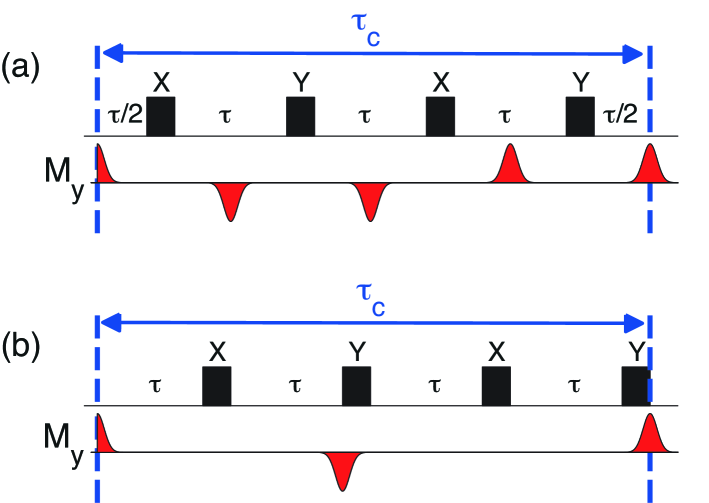
Figure 1: Schematic representation of dynamical decoupling sequences: (a) time symmetric XY-4 and (b) asymmetric XY-4.

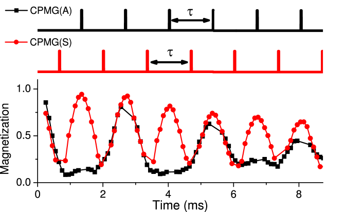
Figure 2: Experimentally observed evolution of the ¹³C nuclear spin magnetization of adamantane during the symmetric (red circles) and asymmetric (black squares) CPMG pulse sequences.

In the spectroscopy and quantum computing communities, two versions of the XY-4 sequence are used that differ by a seemingly minor detail. As shown in Fig. 1a, the basic cycle originally introduced in NMR [33, 40] starts with a delay of duration $\tau/2$ and ends with another delay of the same duration. It therefore shows reflection symmetry in the time domain with respect to the center of the cycle. In contrast to that, the sequence used in the quantum information community [1, 39, 41, 42, 43] starts with a delay of duration $\tau$ and ends after the fourth pulse (see Fig. 1b). Clearly, this cycle is not symmetric in time. One consequence of this small difference is that in the case shown in Fig. 1a, the echoes are formed in the center of the windows between any two pulses, while in Fig. 1b, the echoes coincide with every second pulse. The separation in time between the echoes is therefore twice as long in this case.

Figure 2 illustrates this difference with an experimental example. Here, we measured the time evolution of the ¹³C nuclear spin polarization during a CPMG sequence, using in one case a time-symmetric and in the other case a non time-symmetric cycle. The sample used for this experiment was polycrystalline adamantane. The dephasing of the nuclear spin signal originates from the interaction with an environment consisting of ¹H nuclear spins. To make this environment appear static and generate a long train of echoes, we applied a homonuclear decoupling sequence to the protons [21]. As expected, in the symmetric case, the echoes appear with half the separation of the asymmetric case.

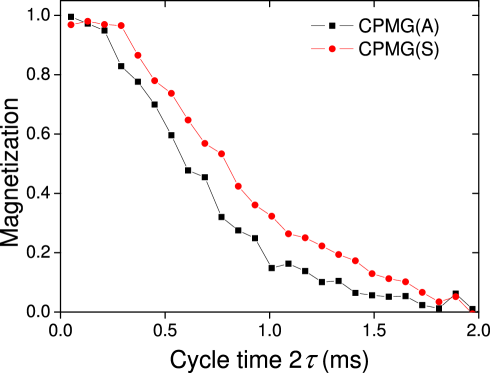
Figure 3: ¹³C nuclear spin magnetization after one cycle of symmetric and asymmetric CPMG sequences for different cycle times 2 $\tau$.

The larger separation of the echoes also can lead to a faster decay of the echo amplitude if the environment is not static. This is illustrated in Fig. 3, which shows the decay of the echo amplitude as a function of time. In this case, we did not apply homonuclear decoupling and the system-environment interaction is therefore modulated by the homonuclear magnetic dipole-dipole interaction between the environmental protons [21]. The plotted signal shows the echo amplitude measured after a single CPMG cycle for the symmetric and asymmetric case, as a function of the cycle time $2\tau$. Clearly the symmetric cycle is more efficient in preserving the state of the system - in agreement with findings from multiple pulse NMR [28, 29].

Since any multiple pulse cycle suffers from imperfections and non-ideal properties, it is often desirable to construct longer cycles that have better properties than simply repeating the basic cycle. Examples of DD sequences that can be constructed from the XY-4 cycle include the XY-8 and XY-16 [40] sequences shown in Table 1. Here, the XY-8 sequence concatenates an XY-4 cycle with its time-reversed version [40, 41, 42, 43], thus generating a new cycle, which is inherently time-symmetric, independent of which version of the XY-4 sequence was used for the building blocks.

In the following sections 3 and 4 we show that two symmetric sequences, constructed according to the same rules from a basic XY-4 block can have different behaviors depending if the basic block is chosen to be symmetric or not.

	Asymmetric	Symmetric
$XY-4$	$[\tau-X-\tau-Y]^{2}$	$[\tau/2-X-\tau-Y-\tau/2]^{2}$
$XY-8$	$(XY-4)(XY-4)^{T}$
$XY-16$	$(XY-8)\overline{(XY-8)}$

Table 1: Dynamical decoupling sequences. The top line shows the time symmetric and asymmetric versions of XY-4, which can be used as building blocks for other sequences. $X$ and $Y$ represent $\pi$-pulses around the $x$ and $y$ axes respectively. $U^{T}$ is the time-reversed sequence and $\overline{U}$ stands for the sequence with inverted phases.

3 Average Hamiltonian Theory

In this section we compare DD sequences constructed from time symmetric and asymmetric building blocks in the framework of average Hamiltonian theory [24, 34]. While the zero-order average Hamiltonian of the asymmetric sequence is the same as that of the symmetric sequence, this is no longer the case for the higher order terms. In particular, if a cycle is symmetric, that is if $\tilde{H}(t)=\tilde{H}(\tau_{c}-t)$ for $0\leq t\leq\tau_{c}$, where $\tilde{H}(t)$ represents the Hamiltonian in the toggling frame [24, 34], it can be shown that all odd order terms of the average Hamiltonian vanish [30]. Clearly, this condition can only be fulfilled, if the timing of the sequence is symmetric, as in the example of Fig. 1a.

We first consider the sequence XY-4, which is our basic building block. Our system consists of a single qubit, which we describe as a spin 1/2, and an environment, which consists of a spin-bath. The Hamiltonian describing the system plus environment is then

$$H=H_{S}+H_{SE}+H_{E},$$ (1)

where $H_{S}=\omega_{S}S_{z}$ is the system Hamiltonian, $\mathbf{S}=(S_{x},S_{y},S_{z})$ is the spin vector operator of the system qubit and $\omega_{S}$ is the Zeeman frequency of the system. $H_{E}$ is the environment Hamiltonian, which does not commute with $H_{SE}$ in general but is not specified further. $H_{SE}$ is the system-environment interaction:

$$H_{SE} = \sum_{k}b_{k}S_{z}I_{z}^{k}.$$ (2)

In the following, we work in a resonant rotating frame, where $\omega_{S}=0$ and therefore $H_{S}=0$. $\mathbf{I^{k}}=(I^{k}_{x},I^{k}_{y},I^{k}_{z})$ is the spin vector operator of the $k^{th}$ environment spin, $b_{k}$ is the coupling constant between the system and the $k^{th}$ spin of the environment.

In our case, the dominant source of experimental imperfections are flip-angle errors. The actual pulse propagator for a nominal $\pi$ rotation around an axis defined by $\phi$ is then

$$R(\phi) = e^{-i(1+\epsilon)\pi S_{\phi}}$$ (3)

where $\epsilon$ is the relative flip angle error, $S_{\phi}=cos\phi S_{x}+sin\phi S_{y}$, and $\phi$ is the phase of the pulse. We can write the zeroth ($\overline{H_{0}}$) and first ($\overline{H_{1}}$) order terms of the average Hamiltonian for the time symmetric XY-4 sequence

$$\overline{H_{0}^{S}} = H_{E}$$ (4)

$$\overline{H_{1}^{S}} = \frac{5\epsilon^{2}\pi^{2}}{16\tau}S_{z}-\sum_{k}b_{k}{\frac{\epsilon\pi}{32}(S_{x}+S_{y})I_{z}^{k}}.$$ (5)

Details of the calculation are given in the appendix. The zeroth order average Hamiltonian matches exactly the target Hamiltonian, and for perfect pulses ($\epsilon=0$), the first order term vanishes, $\overline{H_{1}^{S}}=0$, as expected for any symmetric sequence. For finite pulse errors, the first-order term contains a rotation of the spin qubit around the $z$ axis by an angle $5\epsilon^{2}\pi^{2}/4$. This term results from the accumulated flip angle errors and is independent of the environment. Since this term is proportional to the square of the flip angle error $\epsilon$, it generates a rotation in the same direction for all spins, independent of the actual field that they experience.

The second term in eq. (5), in contrast, is linear in $\epsilon$. For an optimal setting of the pulse, $\epsilon$ is distributed symmetrically around zero and the resulting evolution due to this term does not lead to an overall precession, but to a loss of amplitude. This term combines pulse errors and the system-bath interaction. It arises from the fact that pulses that do not implement a $\pi$ rotation cannot properly refocus the system-environment interaction.

Now we compare these results with the average Hamiltonian of the time asymmetric form of XY-4:

$$\overline{H_{0}^{A}} = H_{E}$$ (6)

$$\overline{H_{1}^{A}} = \frac{5\epsilon^{2}\pi^{2}}{16\tau}S_{z}-\sum_{k}b_{k}\frac{\epsilon\pi}{16}S_{x}I_{z}^{k}$$ (7)

$$+i\tau S_{z}\sum_{k}b_{k}[I_{z}^{k},H_{E}],$$

The most striking difference from the symmetric case is the appearance of a new term which is a commutator between the internal Hamiltonian of the environment $H_{E}$ and the system-environment interaction Hamiltonian $H_{SE}$.

Under ideal conditions, the first-order average Hamiltonian vanishes for the symmetric building block, but not for the asymmetric case. For the asymmetric case the third term, which is proportional to $[H_{SE},H_{E}]$ remains. The commutator describes the time dependence of the system-environment interaction due to the environmental Hamiltonian $H_{E}$. This difference from the symmetric case may be understood in terms of the different positions of the echoes shown in Fig. 1 and Fig. 2: In the asymmetric sequence, the time between echoes is twice as long as in the symmetric sequence, which means that a time-dependent environment has a bigger effect. In the symmetric sequence, the effect of the time-dependent environment appears only in the next-higher order term.

Rules for improving the performance of multiple pulse sequences were discussed, e.g., in the context of broadband heteronuclear decoupling [44] or for the compensated Carr-Purcell sequences [40]. If we combine a XY-4 cycle with its time-reversed image to an XY-8 cycle, we obtain a time-symmetric cycle, even if we start from the non-time symmetric block. Nevertheless, we expect different results for the two cases. An explicit calculation of the average Hamiltonian for the combined cycle shows that $\overline{H_{0}^{S}}=\overline{H_{0}^{A}}=H_{E}$ and $\overline{H_{1}^{S}}=\overline{H_{1}^{A}}=0$, i.e. all deviations from the ideal Hamiltonian vanish to first order. This remains true for finite pulse errors: the symmetry of the sequence cancels the effect of pulse errors in all odd-order average Hamiltonian terms.

We therefore proceed to calculate the second order terms. For simplicity, we do not calculate the general expression, but consider two limiting cases. First, we assume that the environmental Hamiltonian vanishes, $H_{E}=0$. The second order term then becomes

$$\overline{H_{2}^{S}} = \frac{13\epsilon^{3}\pi^{3}}{1536\tau}(S_{x}+S_{y})+\sum_{k}\frac{\epsilon^{2}\pi^{2}b_{k}}{384}S_{z}I_{z}$$ (8)

$$\overline{H_{2}^{A}} = \overline{H_{2}^{S}}+\sum_{k}\frac{\epsilon b_{k}^{2}\tau}{368}S_{y}.$$ (9)

Again, the average Hamiltonian for the sequence built from asymmetric blocks contains an additional error term, which depends on the pulse error and the square of the system-environment interaction.

As the second limiting case, we assume ideal pulses but non-vanishing environmental Hamiltonian, $H_{E}\neq 0$. The second order terms then become

$$\overline{H_{2}^{S}} = \frac{\tau^{2}}{8}[[H_{E},H_{SE}],H_{E}-\frac{1}{3}H_{SE}]$$ (10)

$$\overline{H_{2}^{A}} = \overline{H_{2}^{S}}+\frac{\tau^{2}}{8}[[H_{E},H_{SE}],7H_{E}-H_{SE}].$$ (11)

As for the XY-4 sequence, the time-dependence of the environment, represented by the commutator $[H_{E},H_{SE}]$ has the bigger effect if the sequence uses an asymmetric building block and therefore generates echoes with bigger time delays between them.

4 experimental Results

4.1 Setup and system

For the experimental tests we used natural abundance ¹³C nuclear spins in the CH₂ groups of a polycrystalline adamantane sample as the system qubit. The carbon spins are coupled to nearby ¹H nuclear spins by heteronuclear magnetic dipole interaction corresponding to $H_{SE}$. The protons are coupled to each other by the homonuclear dipolar interaction, which corresponds to $H_{E}$ and does not commute with $H_{SE}$. The system environment interaction is therefore not static and the carbon spins experience a fluctuating environment [18]. Under our conditions, the interaction between the carbon nuclei can be neglected and the decoherence mechanism is a pure dephasing process [18], the evolution of the system and environment is thus described by the Hamiltonian (1).

The experiments were performed on a homebuilt 300 MHz solid-state NMR spectrometer. The basic experimental scheme consisted of: a state preparation period, during which we prepared the carbon spins in a superposition state oriented along the $y$ direction, a variable evolution period, where DD sequences were applied, and the final read out period where we determine the final state by quantum state tomography [35, 36].

Figure 4: Decay of the $M_{y}$-magnetization for the symmetric version of XY-4 and different delays ($\tau$) between pulses.

Figure 4 shows the signal decay for the symmetric version of XY-4 and different delays $\tau$ between the refocusing pulses. For the shortest cycle times, we observe shorter decays and oscillations. As discussed in Ref. [18], this is an indication that in this regime pulse imperfections play the dominant role. From the decay curves, we extract decay times as the times where the magnetization has decayed to $1/e$ of the initial value.

4.2 Measured decay times

Figure 5 shows the decay times of the $M_{y}$-magnetization as a function of the delay $\tau$ between the pulses. For delays between 200 $\mu$s and 50 $\mu$s, the decoupling performance improves as the delays between the pulses are reduced. However, as the delay between the pulses becomes shorter than 50 $\mu$s, the decay time decreases again, in agreement with what was observed in [18, 22]: in this region, pulse errors become more important than the coupling to the environment. This occurs equally for both, the symmetric and the asymmetric XY-4 sequence.

If we concatenate the XY-4 sequence with its time-reversed version to the XY-8 sequence, we obtain qualitatively different behavior for the two different versions of XY-4: If we start from the symmetric form of XY-4, the resulting XY-8(S) sequence shows improved decoupling performance for increasing pulse rate, without saturating. This is a clear indication that in this case, the concatenation eliminates the effect of pulse imperfections and generates a robust, well-compensated sequence. In strong contrast to this, concatenation of the asymmetric version of XY-4 to XY-8(A) does not lead to a significant improvement: the decay times for XY-8(A) are identical to those of the two XY-4 sequences, within experimental uncertainty. A further concatenation to XY-16 does not change this behavior. The qualitatively different behavior of the sequences using symmetric versus asymmetric building blocks clearly shows that for the asymmetric versions, the pulse errors dominate, while the symmetric ones compensate for the effect of pulse errors.

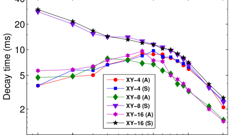
Figure 5: Decay time of the $M_{y}$-magnetization for different XY-$n$ sequences.

4.3 Tomographic analysis

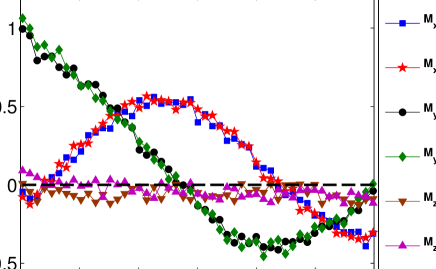
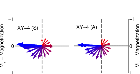
Figure 6: Evolution of the magnetization during the symmetric (A) and asymmetric (S) versions of the XY-4 sequence for pulse spacings of $\tau=10\mu s$. The top panel shows the evolution of the magnetization components as a function of time. The bottom panel represents the Bloch vector in the $xy$ plane at different times. The color code in the lower panel denotes the time evolution, blue for the initial state and red for the final state.

For a more detailed picture of the process that reduces the signal for high pulse rates, we applied state tomography of the evolving qubit by measuring all three components along the $x$, $y$ and $z$-direction. Figure 6 shows the observed data for both versions of the XY-4 sequence. The oscillation of the $x$- and $y$ components and the constantly small value of the $z$-component are a clear indication of a precession around the $z$-axis, in addition to the loss of signal amplitude. This combination of precession and reduction of amplitude is also shown in the lower part of Fig. 6, where the arrows show the xy-components of the magnetization for different times during the sequence. According to eqs (5) and (7), the precession around the $z$-axis originates from the pulse error term $5\epsilon^{2}\pi^{2}/(16\tau)S_{z}$, which is proportional to $\epsilon^{2}$ and is the same for the symmetric and the asymmetric sequence, in excellent agreement with the observed behavior.

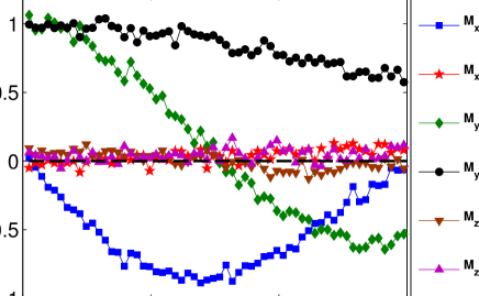
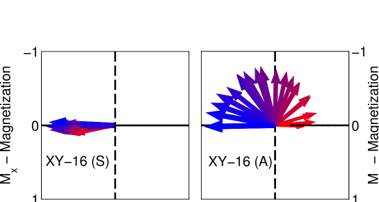
Figure 7: Evolution of the magnetization during the symmetric (A) and asymmetric (S) versions of the XY-16 sequence for pulse spacings of $\tau=10\mu s$. The top panel shows the evolution of the magnetization components as a function of time. The bottom panel represents the Bloch vector in the $xy$ plane at different times. The color code is the same as in Fig. 6.

Figure 7 shows the corresponding data for the two XY-16 sequences. Here, as well as in the case of XY-8 (data not shown), we also observe a precession for the XY-16(A) sequence, but for the sequence with symmetric building blocks, the oscillation is not observed. Again, these results indicate that the sequences built from symmetric XY-4 blocks have smaller average Hamiltonians and therefore show better performance than those built from asymmetric blocks.

If we change the spacing between the pulses, the behavior remains the same. In Fig. 8, we show the measured precession angle around the $z$-axis divided by the number of pulses. The precession is indistinguishable from zero for the compensated XY-8(S) and XY-16(S) sequences. For other sequences, it is significant and independent of the delay between the pulses.

The precession of the magnetization around the $z$-axis that we observe for some of the sequences causes a deviation of the system from the desired evolution and reduces therefore the fidelity of the process. However, compared to a dephasing process, it is easier to correct and can in principle be compensated if it is known. We therefore compared not only the reduction of the magnetization amplitude along the initial direction, but also the total magnetization left in the system, which eliminates the effect of the precession. Figure 9 shows the decay times of the total magnetization for different XY-$n$ sequences. For short delays between the pulses, the difference between sequences built by symmetric and asymmetric building blocks is small, indicating that the main difference is related to the precession originating from the pulse errors, which is better compensated by concatenating symmetric building blocks. For pulse delays longer than $\tau\approx 15\mu$s, we start to see again that the symmetric versions of XY-8(S) and XY-16(S) are superior to the asymmetric versions. At this point, the time dependence of the environment plays a bigger role and reduces the efficiency of the refocusing [18, 22]. In agreement with eqs (9) and (11), these effects are bigger for those sequences that use asymmetric building blocks.

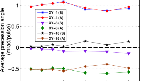
Figure 8: Average precession angle of the transverse magnetization during the different XY-$n$ sequences.

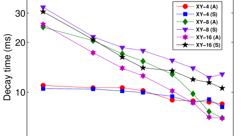
Figure 9: Decay time of the total magnetization for XY-$n$ sequences.

5 Discussion and Conclusions

Dynamical decoupling is becoming a standard technique for extending the lifetime of quantum mechanical coherence. Many different sequences have been put forward for reducing the effect of the environmental noise on the system. Since the number of possible sequences is infinite, a relatively straightforward approach for designing improved sequences consists in concatenating different building blocks in such a way that the resulting cycle has a smaller overall average Hamiltonian than that of its component blocks. In this paper we consider the XY-4 sequence as a basic building block. Since different versions of the XY-4 sequence were proposed in the literature, some of them symmetric in time, others asymmetric, we compare these two versions and in particular the different sequences that result when they are concatenated with time-inverted and phase-shifted copies. Since time-symmetric sequences generate average Hamiltonians in which all odd-order terms vanish for ideal pulses, it is expected that they perform better than non-symmetric but otherwise identical sequences. Experimentally, we could not verify this for the XY-4 sequence, since pulse errors dominate the behavior under our experimental conditions. However, in the case of the CPMG sequence, where pulse errors are insignificant, we could clearly verify this expectation.

The symmetry of the basic building blocks is also important when they are concatenated to higher order sequences, such as the XY-8 and XY-16 sequences [40]. In this case, the odd order terms vanish in the average Hamiltonians of both sequences, but the second order terms of the sequences that are built from asymmetric blocks contain additional unwanted terms. The experimental data are in agreement with this observation: sequences consisting of time symmetric building blocks perform significantly better than the corresponding sequences formed by time asymmetric blocks.

In order to understand the decay processes during the DD sequences, we performed quantum state tomography as a function of time. The results from these measurements show two different contributions to the overall fidelity loss: A precession around the $z$-axis, which we could attribute to the combined effect of flip-angle errors and an overall reduction of the amplitude, which results from the system-environment interaction. For short delays between the pulses and correspondingly large number of pulses, the pulse error term is the dominating effect. Again, the symmetric and asymmetric version of the XY-4 sequence show similar performance. However, as we use them as building blocks of the higher-order XY-8 and XY-16 sequences, we find that the effect of the pulse errors is almost perfectly compensated if we use the symmetric building blocks, while a significant effect remains when asymmetric blocks are concatenated.

While we have analyzed the effect of symmetry mostly for the XY-$n$ sequences, this can clearly be generalized. As we showed in Fig. 3, the symmetric version of the CPMG sequence shows significantly better decoupling performance than the asymmetric version. The same concept can also be applied to the CDD sequences, which are generated by inserting XY-4 sequences inside the delays of a lower-order CDD sequence [39]. The conventional concatenation scheme [39] uses asymmetric building blocks. Here, we used the symmetric XY-4 sequence as the building-blocks, and we modified the concatenation scheme in such a way that the symmetry is preserved and the delays between the pulses are identical at all levels of concatenation. The conventional (asymmetric) version CDD_n(A) is iterated as $[CDD_{n-1}-X-CDD_{n-1}-Y]^{2}$. In contrast to that, we construct the symmetrized version CDD_n(S) as $[\sqrt{CDD_{n-1}}-X-CDD_{n-1}-Y-\sqrt{CDD_{n-1}}]^{2}$ [22]. For $n=1$, we have $CDD_{1}$ = XY-4. In Fig. 10 we compare the process fidelities [45, 46] for the two versions of the CDD-2 sequence. Clearly, the symmetrized version CDD₂(S) shows a significantly improved performance, compared to the standard, asymmetric version CDD₂(A).

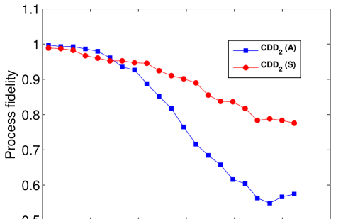
Figure 10: Process fidelities of the symmetric vs. asymmetric version of CDD-2 as a function of time for an average delay $\tau=12.5\mu\mathrm{s}$ between the refocusing pulses.

The results presented in this paper show clearly that it is time reversal symmetry is a useful tool for improving dynamic decoupling sequences. The symmetric sequences often perform better and never worse than non-symmetric sequences, at no additional cost.

References

Appendix A Average Hamiltonian Calculation

In this Appendix we show how the average Hamiltonian was calculated. The essence of average-Hamiltonian theory is that a cyclic evolution, $U(t)$, can be described by an effective evolution governed by a time-independent Hamiltonian $\overline{H}$. When $U$ is comprised by a sequence of unitary operations, i.e. $U=e^{O_{n}}\cdots e^{O_{2}}e^{O_{1}}$, the average Hamiltonian can be approximately computed by recursive applications of the Baker-Campbell-Hausdorff formula

$$log(e^{A}e^{B}) \approx A+B+\frac{1}{2}[A,B]+$$ (12)

$$\frac{1}{12}\left([A,[A,B]]+[[A,B],B]\right)$$

To approximate the average Hamiltonian of the XY-4 sequence, consider the following sequence:

$$[\tau_{i}-R_{1}-\tau-R_{2}-\tau-R_{3}-\tau-R_{4}-\tau_{f}],$$ (13)

where $R_{1}=R_{3}=R(X)$, $R_{2}=R_{4}=R(Y)$ and $R({\phi})$ is a the pulse propagator defined in Eq. 3. In the asymmetric form of XY-4, $\tau_{i}=\tau$ and $\tau_{f}=0$. For $\tau_{i}=\tau_{f}=\tau/2$, we obtain the symmetric form of XY-4. The total sequence propagator is

$$U = e^{-iH\tau_{f}}\left(\prod_{k=2}^{4}R_{k}e^{-iH\tau}\right)R_{1}e^{-iH\tau_{i}},$$ (14)

where $H$ is the Hamiltonian of Eq. (1).

To account for flip angle errors, we decompose the propagator into a product of the ideal pulse propagator sandwiched between two additional evolutions:

$$R_{\phi} = e^{-i(1+\epsilon)\pi S_{\phi}}$$ (15)

$$= e^{-iH_{\phi}\frac{t_{p}}{2}}e^{-i\pi S_{\phi}}e^{-iH_{\phi}\frac{t_{p}}{2}}$$

where $H_{\phi}=\frac{\epsilon\pi}{t_{p}}S_{\phi}$ and $t_{p}$ is pulse length. Substituting equation (15) in (14) and using the following approximation:

$$e^{-iH_{\phi}\frac{t_{p}}{2}}e^{-iH\tau} \approx e^{-i(H\tau+H_{\phi}\frac{t_{p}}{2})}$$ (16)

$$\approx e^{-i(H+\frac{1}{2\tau}\epsilon\pi S_{\phi})\tau}$$

$$\approx e^{-iH^{{}^{\prime}}\tau},$$

the new sequence propagator is then rewritten as

$$U = e^{-iH_{5}^{{}^{\prime}}\tau_{f}}\left(\prod_{k=2}^{4}R_{k}e^{-iH_{k}^{{}^{\prime}}\tau}\right)R_{1}e^{-iH_{1}^{{}^{\prime}}\tau_{i}},$$ (17)

where

$$\tau_{i}H_{1}^{{}^{\prime}} = \tau_{i}H+\frac{t_{p}}{2}H_{X}$$ (18)

$$\tau H_{k=2,3,4}^{{}^{\prime}} = \tau H+\frac{t_{p}}{2}\left(H_{X}+H_{Y}\right)$$ (19)

$$\tau_{f}H_{5}^{{}^{\prime}} = \tau_{i}H+\frac{t_{p}}{2}H_{Y}.$$ (20)

The calculation can be simplified by transforming the Hamiltonians to a new frame after each pulse, the so-called toggling frame. The Hamiltonians $\widetilde{H_{k}}$ in this new frame are given by:

$$\tau_{i}\widetilde{H_{1}} = \tau_{i}(H_{E}+H_{SE})+\frac{t_{p}}{2}H_{X}$$ (21)

$$\tau\widetilde{H}_{k=2,3,4} = \tau[H_{E}+(-1)^{k+1}H_{SE}]$$ (22)

$$-t_{p}[(2\delta_{k,2}+1)H_{X}+(2\delta_{k,4}+1)H_{Y}]$$

$$\tau_{f}\widetilde{H_{5}} = \tau_{f}(H_{E}+H_{SE})+\frac{t_{p}}{2}H_{Y}$$ (23)

and the sequence propagator is:

$$U\approx\prod_{k=1}^{5}e^{-i\widetilde{H_{k}}\tau_{k}}$$ (24)

The final step consists of the recursive applications of eq. (12) to eq. (24). An explicit calculation of the zeroth and first order terms leads to the equations (4) and (5) for the symmetric case and (6) and (7) for the asymmetric case. The calculation for XY-8 follows the same procedure as described for XY-4. Here the sequence is comprised by eight pulses and nine delays (see table 1), this leads to the total propagator analog to 17:

$$U = e^{-iH_{9}^{{}^{\prime}}\tau_{f}}\left(\prod_{k=2}^{8}R_{k}e^{-iH_{k}^{{}^{\prime}}\tau}\right)R_{1}e^{-iH_{1}^{{}^{\prime}}\tau_{i}},$$ (25)

Transforming the Hamiltonians $H_{k}^{{}^{\prime}}$ to the toggling frame, one can show that $\widetilde{H_{k}}=\widetilde{H}_{1-k}$, the Hamiltonians $\widetilde{H}_{k=1,2,3,4}$ are the same as in Eqs. (21) - Eqs. (22) and $\tau\widetilde{H_{5}}=\tau(H_{E}+H_{SE})+t_{p}H_{Y}$.

References

- [1] L. Viola, E. Knill, and S. Lloyd. Dynamical decoupling of open quantum systems. Phys. Rev. Lett., 82:2417, 1999.
- [2] Wen Yang, Zhen-Yu Wang, and Ren-Bao Liu. Preserving qubit coherence by dynamical decoupling. Front. Phys., 6:1, 2010.
- [3] K. Khodjasteh and L. Viola. Dynamically error-corrected gates for universal quantum computation. Phys. Rev. Lett., 102:080501, Feb 2009.
- [4] K. Khodjasteh, D. A. Lidar, and L. Viola. Arbitrarily accurate dynamical control in open quantum systems. Phys. Rev. Lett., 104:090501, Mar 2010.
- [5] J. R. West, D.A. Lidar, B. H. Fong, and M. F. Gyure. High fidelity quantum gates via dynamical decoupling. Phys. Rev. Lett., 105:230503, Dec 2010.
- [6] H .K. Ng, D. A. Lidar, and J. Preskill. Combining dynamical decoupling with fault-tolerant quantum computation. Phys. Rev. A, 84:012305, Jul 2011.
- [7] Sergio Boixo and Rolando D. Somma. Parameter estimation with mixed-state quantum computation. Phys. Rev. A, 77:052320, May 2008.
- [8] J. Bylander, S. Gustavsson, F. Yan, F. Yoshihara, K. Harrabi, G. Fitch, D. G. Cory, Y. Nakamura, J-S Tsai, and W. D. Oliver. Noise spectroscopy through dynamical decoupling with a superconducting flux qubit. Nat. Phys., 7:565, 2011.
- [9] I. Almog, Y. Sagi, G. Gordon, G. Bensky, G. Kurizki, and N. Davidson. Direct measurement of the system-environment coupling as a tool for understanding decoherence and dynamical decoupling. J. Phys. B: At. Mol. Opt. Phys., 44(15):154006, 2011.
- [10] G. A. Alvarez and D. Suter. Dynamical decoupling noise spectroscopy. arXiv:1106.3463 (2011) (Submitted).
- [11] J. M. Taylor, P. Cappellaro, L. Childress, L. Jiang, D. Budker, P. R. Hemmer, A. Yacoby, R. Walsworth, and M. D. Lukin. High-sensitivity diamond magnetometer with nanoscale resolution. Nat. Phys., 4:810, 2008.
- [12] C. A. Meriles, L. Jiang, G. Goldstein, J. S. Hodges, J. Maze, M. D. Lukin, and P. Cappellaro. J. Chem. Phys., 133:124105, 2010.
- [13] L. T. Hall, C. D. Hill, J. H. Cole, and L. C. L. Hollenberg. Ultrasensitive diamond magnetometry using optimal dynamic decoupling. Phys. Rev. B, 82:045208, Jul 2010.
- [14] G. de Lange, D. Ristè, V. V. Dobrovitski, and R. Hanson. Single-spin magnetometry with multipulse sensing sequences. Phys. Rev. Lett., 106:080802, Feb 2011.
- [15] J. Du, X. Rong, N. Zhao, Y. Wang, J. Yang, and R. B. Liu. Preserving electron spin coherence in solids by optimal dynamical decoupling. Nature, 421:1265, 2009.
- [16] M. J. Biercuk, H. Uys, A. P. VanDevender, N. Shiga, W. M. Itano, and J. J. Bollinger. Optimized dynamical decoupling in a model quantum memory. Nature, 458:996, 2009.
- [17] E. R. Jenista, A. M. Stokes, R. T. Branca, and W. S. Warren. Optimized, unequal pulse spacing in multiple echo sequences improves refocusing in magnetic resonance. J. Chem. Phys., 131:204510, 2009.
- [18] G. A. Álvarez, A. Ajoy, X. Peng, and D. Suter. Performance comparison of dynamical decoupling sequences for a qubit in a rapidly fluctuating spin bath. Phys. Rev. A, 82:042306, 2010.
- [19] G. deLange, Z. H. Wang, D. Risté, V. V. Dobrovitski, and R. Hanson. Universal dynamical decoupling of a single solid-state spin from a spin bath. Science, 330:60, 2010.
- [20] C. A. Ryan, J. S. Hodges, and D. G. Cory. Robust decoupling techniques to extend quantum coherence in diamond. Phys. Rev. Lett., 105:200402, 2010.
- [21] Ashok Ajoy, Gonzalo A. Álvarez, and Dieter Suter. Optimal pulse spacing for dynamical decoupling in the presence of a purely dephasing spin bath. Phys. Rev. A, 83(3):032303, Mar 2011.
- [22] A. M. Souza, G. A. Álvarez, and D. Suter. Robust dynamical decoupling for quantum computing and quantum memory. Phys. Rev. Lett., 106:240501, 2011.
- [23] Z-H. Wang and V. Dobrovitski. Aperiodic dynamical decoupling sequences in the presence of pulse errors. J. Phys. B: At. Mol. Opt. Phys., 44:154004, 2011.
- [24] U. Haeberlen and J. S. Waugh. Coherent averaging effects in magnetic resonance. Phys. Rev., 175:453–467, Nov 1968.
- [25] P. Mansfield. Symmetrized pulse sequences in high resolution nmr in solids. J. Phys. C: Solid State Phys., 4(11):1444, 1971.
- [26] W. K. Rhim, D. D. Elleman, and R. W. Vaughan. Analysis of multiple pulse nmr in solids. J. Chem. Phys., 59:3740, 1973.
- [27] D. P. Burum and W. K. Rhim. Analysis of multiple pulse nmr in solids ii. J. Chem. Phys., 71:944, 1979.
- [28] M. H. Levitt. J. Chem. Phys., 128:052205, 2008.
- [29] M. H. Levitt. Symmetry-based pulse sequences in magic-angle spinning solid-state nmr. In Encyclopedia of NMR (Wiley, 2002).
- [30] D. P. Burum. Magnus expansion generator. Phys. Rev. B, 24:3684, 1981.
- [31] A. J. Shaka and A. Pines. J. Magn. Reson., 71:495, 1987.
- [32] J. T. Ngo and P. G. Morris. J. Magn. Reson., 74:122, 1987.
- [33] A.A Maudsley. Modified carr-purcell-meiboom-gill sequence for nmr fourier imaging applications. J. Magn. Reson., 69(3):488, 1986.
- [34] R. R. Ernst, G. Bodenhausen, and A. Wokaum. Principles of nuclear magnetic resonance in one and two dimensions. Clarendon Press, United Kingdom, 1987.
- [35] I. L. Chuang, N. Gershenfeld, M. G. Kubinec, and D. W. Leung. Bulk quantum computation with nuclear magnetic resonance: theory and experiment. Proc. R. Soc. Lond. A, 454:447, 1998.
- [36] I. S. Oliveira, R. S. Sarthour, E. R. deAzevedo, T. J. Bonagamba, and J. C. C. Freitas. NMR Quantum information processing. Elsevier, Netherland, 2007.
- [37] H. Y. Carr and E. M. Purcell. Effects of diffusion on free precession in nuclear magnetic resonance experiments. Phys. Rev., 94:630–638, May 1954.
- [38] S. Meiboom and D. Gill. Modified spin echo method for measuring nuclear relaxation times. Rev. Sci. Instrum., 29:688, 1958.
- [39] K. Khodjasteh and D. A. Lidar. Fault-tolerant quantum dynamical decoupling. Phys. Rev. Lett., 95:180501, 2005.
- [40] T. Gullion, D. B. Baker, and M. S. Conradi. New compensated carr-purcell sequences. J. Magn. Reson., 89:479, 1990.
- [41] K. Khodjasteh and D. A. Lidar. Performance of deterministic dynamical decoupling schemes: Concatenated and periodic pulse sequences. Phys. Rev. A, 75:062310, 2007.
- [42] L. F. Santos and L. Viola. New J. Phys., 10:083009, 2008.
- [43] H. K. Ng, D. A. Lidar, and J. Preskill. Combining dynamical decoupling with fault-tolerant quantum computation. Phys. Rev. A, 84:012305, Jul 2011.
- [44] M. H. Levitt, R. Freeman, and T. Frenkiel. J. Magn. Reson., 50:157, 1982.
- [45] I. L. Chuang and M. A. Nielsen. Prescription for experimental determination of the dynamics of a quantum black box. J. Mod. Opt., 44:2455, 1997.
- [46] M. A. Nielsen and I. L. Chuang. Quantum Computation and Quantum Information. Cambridge University Press, Cambridge, 2000.