Bending of bilayers with general initial shapes

Abstract

We present a simple discrete formula for the elastic energy of a bilayer. The formula is convenient for rapidly computing equilibrium configurations of actuated bilayers of general initial shapes. We use maps of principal curvatures and minimum-curvature direction fields to analyze configurations. We find good agreement between the computations and an approximate analytical solution for the case of a rectangular bilayer. For more general shapes (simple polyiamonds), we find a range of typical bending behaviors: overall bending directions along longest and shortest dimensions, inward bending at corners, curvature intensification near boundaries, and conical bending and partitioned bending zones in some cases.

I Introduction

A bilayer is a thin sheet consisting of two layers, each composed of a different material. When the environment external to the bilayer undergoes a change in temperature or chemical composition, the equilibrium strains of the two layers change by different amounts due to their different material properties timoshenko1925analysis . In one common type of bilayer smela1993electrochemical , one layer, called the substrate, has an equilibrium strain of zero throughout the external environmental change. The other layer, called the actuated layer, has an equilibrium strain which changes from zero to a (possibly nonuniform) value $\epsilon_{a}$. Because the layers are bonded, they undergo the same strain at their interface, and thus both layers cannot simultaneously be uniformly at their equilibrium strains. However, each layer can be brought closer to its equilibrium strain, on average, when the bilayer bends. Then the layer along the outer circumference is stretched relative to the inner layer, so the average strain in each layer is different.

Bilayers are a widely-used technology for producing precisely-controllable motions and shape changes for solid bodies. A common application is the household thermostat timoshenko1925analysis , and newer applications include self-assembling containers smela1995controlled ; leong2008thin , biomedical devices smela2003conjugated , and radio-frequency switches for wireless communications guerre2010wafer . Bilayers can be considered as a method for making new three-dimensional structures by inducing in-plane stress. Recent work has used imposed stresses in deformable membranes to create wrinkled patterns sharon2007geometrically ; huang2010smooth and other buckled and twisted shapes klein2007shaping ; armon2011geometry .

In this study we extend a model for thin homogeneous elastic sheets to bilayers. The previous model has been used to study a wide range of physical problems, including elastic strains due to defects in materials Seung:1988 , the crumpling of paper Lobkovsky:1997 , the self-assembly of elastic sheets under magnetic forces alben2007self , and the bending and buckling of spheroidal pollen grains under osmotic pressure katifori2010foldable . The simplicity of the model has made it very easy to apply to a wide range of problems.

The present model represents the bending of a bilayer in terms of a mesh for just a single surface—the central surface of the substrate layer. In terms of the shape of this surface, we derive a discrete local formula for the strain in the central surface of the actuated layer. Simple formulas for the elastic energy and its gradient are then obtained, which can be used to find bilayer shapes as energy minima using standard optimization methods. The computational cost of simulating a bilayer in this way is only slightly higher than that of simulating a homogeneous elastic sheet, because the strain in the central surface of the actuated layer is proportional to the curvature of the substrate.

The organization of the paper is as follows. In section II, we derive the bilayer model. In section III we present sample simulations of a rectangular bilayer, and compare with an approximate analytical solution. Section IV presents examples of bilayer bending for various bilayer shapes, most of which are simple polyiamonds. Section V summarizes the results.

II Model

We represent a bilayer in discretized form using a triangular mesh. The mesh is an equilateral triangular lattice in the undeformed state. The substrate layer has stretching and bending energies which approximate those of a uniform, isotropic elastic sheet. Both energies may be obtained by summing simple quantities over the edges of the lattice Seung:1988 . The stretching energy is

$$E_{s}=\frac{1}{2}C_{s}\sum_{i,j}\left(|{\mathbf{r}}_{i}-{\mathbf{r}}_{j}|-d_{eq}\right)^{2}.$$ (1)

Here $C_{s}$ is a stretching stiffness constant, $d_{eq}$ is the length of the edges in the undeformed mesh, and the sum is over distinct nearest-neighbor pairs of points. The bending energy is

$$E_{b}=C_{b}\sum_{\alpha,\beta}(1-{\mathbf{n}}_{\alpha}\cdot{\mathbf{n}}_{\beta}).$$ (2)

$C_{b}$ is a bending stiffness constant, and the sum is over distinct nearest-neighbor pairs of triangles, with the unit normal vectors to each triangle given by ${\mathbf{n}}_{\alpha}$ and ${\mathbf{n}}_{\beta}$. In the undeformed state, the mesh lies in the $x$-$y$ plane, and all of the normal vectors are $\mathbf{\hat{e}}_{z}$ (i.e. pointing upwards in the $z$ direction). The normal vector maintains the same direction with respect to its triangle during deformations.

Seung and Nelson showed that when the stretching strain is small and the radii of curvature of the sheet are large relative to $d_{eq}$, $E_{s}$ and $E_{b}$ converge to the stretching and bending energies of a uniform isotropic elastic sheet with Poisson ratio $\nu$ = 1/3 landau1986te ; Seung:1988 . If the (3D) Young’s modulus of the sheet is $E$ and its thickness is $h$, then $C_{s}$ and $C_{b}$ are proportional to the 2D Young’s modulus and the bending modulus of the sheet:

$$C_{s}=\frac{\sqrt{3}}{2}Eh\,;\quad C_{b}=\frac{2}{\sqrt{3}}\frac{Eh^{3}}{12(1-\nu^{2})}.$$ (3)

The substrate and actuated layers are assumed to have uniform thicknesses which are both equal to $h$, and the same stretching and bending stiffness constants, for simplicity. In the initial configuration, the lower surface of the substrate layer lies in the plane $z=-h/2$ and the upper surface lies in the plane $z=h/2$. The lower surface of the actuated layer is bonded to the upper surface of the substrate layer at $z=h/2$, and the upper surface of the actuated layer lies in the $z=3h/2$ plane. Throughout the bilayer in its initial, flat configuration, there are planar and parallel surfaces of material, lying in the planes of constant $z$ between $-h/2$ and $3h/2$. As the bilayer bends, these surfaces of material are no longer planar, but are assumed to remain parallel. This assumption underlies the classical theories of the bending of thin plates and bilayers (including the continuum versions of (1) and (2)), and allows the configuration of the bilayer to be expressed entirely in terms of the configuration of the central surface of the substrate (i.e. the material initially lying in the plane $z=0$). The central surfaces of the substrate and actuated layers may be assumed to remain parallel under large deformations, as long as the thickness of the bilayer is small compared to its radii of curvature at all points, in all directions.

The aforementioned triangular mesh represents the central surface of the substrate (i.e. the material initially lying in the plane $z=0$). The central surface of the actuated layer is parallel to that of the substrate, and displaced from it by a distance $h$ in the direction of the substrate surface normal $\mathbf{n}$.

The actuated layer is actuated by setting its equilibrium stretching strain (uniformly here) to $\epsilon_{a}$, while the equilibrium strain remains zero for the substrate. Bending causes different stretching strains to occur in the central surfaces of the substrate and actuated layers, and thereby allows each surface to move closer to its own equilibrium stretching strain. If the substrate central surface has curvature $\kappa$ in a certain direction at a point, then the strain in the central surface of the actuated layer in that direction is that at the corresponding point in the substrate plus $h\kappa$ (see appendix A). We consider the central surface of the actuated layer to be discretized by a triangular mesh of points, which are those in the substrate mesh plus $h\mathbf{n}$. Then the strain in the actuated layer mesh can be written in terms of that in the substrate mesh. Hence only the substrate mesh is required to characterize the full bilayer geometry. The lengths of edges in the actuated layer mesh are those of the corresponding edges in the substrate mesh, plus the stretching induced by bending in the direction of the edge. This stretching is a discrete approximation of the stretching strain $h\kappa$, times the edge length. In appendix B we derive a discrete formula for the edge stretching by using a locally-quadratic approximation for the bilayer surface centered at midpoint of each edge. The formula is:

$$\mbox{Stretching due to bending}\approx\frac{h\sqrt{3}}{4}\sum_{k=1}^{4}\varphi_{k},$$ (4)

where the angles $\varphi_{k}$ are those between the normals of the four triangles adjacent to the two triangles which share the edge whose stretching is given. These angles are shown schematically in figure 16. The formula for the stretching energy of the actuated layer is then:

$$E_{s,a}=\frac{1}{2}C_{s}\sum_{i,j}\left(|{\mathbf{r}}_{i}-{\mathbf{r}}_{j}|+\frac{h\sqrt{3}}{4}\sum_{k=1}^{4}\varphi_{k}-d_{eq}-\epsilon_{a}d_{eq}\right)^{2}.$$ (5)

Equation (5) is similar to (1), but includes the additional stretching due to bending in the actuated layer (4), and the equilibrium stretching in the actuated layer $\epsilon_{a}d_{eq}$. In the outer sum in $E_{s,a}$, we omit the contribution from edges which are close to the boundary of the mesh, for which not all four of the angles {$\varphi_{k}$} are defined. An alternative would be to use one-sided approximations for the stretching due to bending near the boundary, which may give a higher order of accuracy, at the expense of increased complexity of the scheme. To fully realize the increased accuracy in arbitrary initial planar geometries, an unstructured triangular mesh may be preferred. However, one of the main benefits of our approach is its simplicity.

The bending energy of the actuated layer is close to that of the substrate layer. In appendix A we show that the curvature $\kappa_{a}$ in a given direction along the central surface of the actuated layer is the same as the curvature of the substrate (at the corresponding point and same direction), up to a relative error of $h\kappa$. Since $h\kappa\ll 1$ by assumption in our large deformation plate theory, we take the curvature of the actuated layer to be that of the substrate. The bending energy of the actuated layer is then the same as (2).

The total elastic energy of our model bilayer is then

$$E_{T}=E_{s}+E_{s,a}+2E_{b}.$$ (6)

III Rectangular bilayers

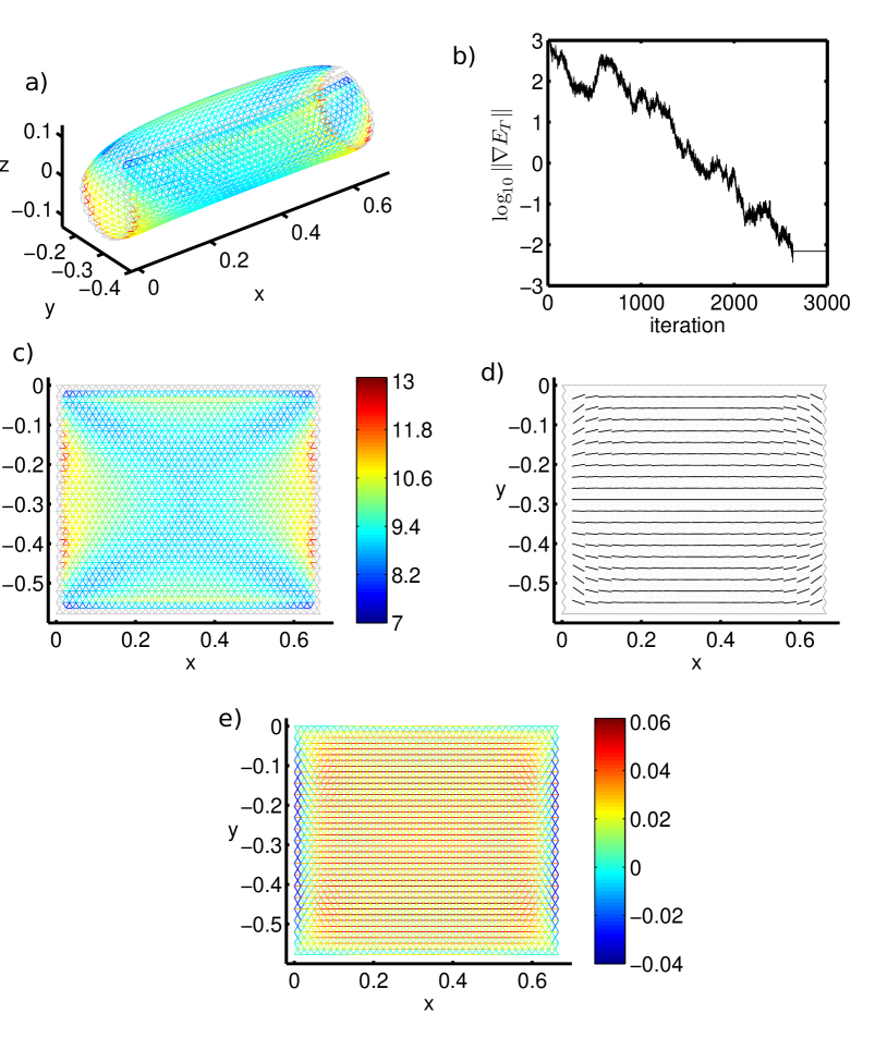
Figure 1: Bending of a rectangular bilayer discretized with 1661 points and 4820 edges. The stretching stiffness $C_{s}$ is $8\times 10^{4}$, and the bending stiffness $C_{b}$ is 1. The thickness is $h$ = 0.01, the initial height (along $y$) is $\sqrt{3}/3$, the initial width (along $x$) is $2/3$. The actuation strain $\epsilon_{a}$ is 10$h$. a, Configuration of rectangular sheet in equilibrium, with bending along the shorter dimension. b, 2-norm of energy gradient versus iteration number in LM-BFGS method, leading up to stagnation, when the equilibrium is reached. c, Color map of maximum principal curvature at the midpoints of edges. Gray edges are too close to the boundary to obtain estimates. d, Direction field showing the directions of minimum principal curvature at the midpoints of edges. e, Color map of stretching strain in each edge of the substrate central surface.

We now test our scheme for perhaps the simplest bilayers—rectangular bilayers—which have been studied previously timoshenko1925analysis ; christophersen2006characterization ; alben2011edge . We first consider a rectangular bilayer which is nearly square—aspect ratio $=\sqrt{3}/2=0.866$. The stretching stiffness $C_{s}$ is $8\times 10^{4}$, and the bending stiffness $C_{b}$ is 1. By (3), we then have that the thickness of each layer $h$ is 0.01. The height and width are of order one ($\sqrt{3}/3$ and $2/3$ respectively), so we have a thin sheet. We set $\epsilon_{a}$ to $10h$. At equilibrium, $h\kappa$ is the strain in the actuated layer due to bending in the substrate, and this should be comparable to $\epsilon_{a}$. Thus we expect $\kappa$ of about 10.

We use a mesh with equilibrium edge length $1/60$, yielding a discretization with 1661 points (4983 degrees of freedom) and 4820 edges. We use a large-scale quasi-Newton scheme to minimize the discrete energy (6), the limited-memory Broyden-Fletcher-Goldfarb-Shanno (LM-BFGS) method with a cubic line search. We use an exact formula for the gradient of $E_{T}$ which can be computed quickly. An exact gradient formula handles large differences in elastic constants better than a finite difference approximation. The initial guess for the minimization routine is the flat state. In figure 1a we show the equilibrium reached by the minimization scheme after it stagnates at about 2500 iterations. The sheet has curled along its shorter dimension, yielding a “cigar” shape, one of two equilibria previously found for rectangular bilayers alben2011edge . The decrease of the 2-norm of $\nabla E_{T}$ with iteration number is shown in panel b, and at stagnation, no further decrease of $E_{T}$ is obtained along the steepest descent direction $-\nabla E_{T}$. At stagnation, the 2-norm of $\nabla E_{T}$ is $7\times 10^{-3}$, and the $\infty$-norm is $4\times 10^{-4}$.

Panel c gives a color map showing the larger of the two principal curvatures at the midpoints of the edges in the equilibrium configuration in ‘a’. Here the bilayer is shown in its initial flat state for clarity. The colors of the edges are the same in ‘a’ and ‘c’, so the correspondence between points on the initial and final shape can be seen. We estimate the principal curvatures using the method described in appendix C. The estimate can be obtained for all edges except those adjacent to the boundary. Over most of the bilayer the maximum principal curvature lies between 8.5 and 10.5. Near the boundary, there is more variation. Panel d gives a field of line segments showing the directions of minimum-magnitude principal curvature at the edge midpoints. For a developable surface, the minimum-magnitude principal curvature is zero at each point. The zero-curvature direction field has integral curves that are straight lines, called generators, which cover the surface struik1988lectures . The shape in panel a (and the other equilbrium shapes in this work) are approximately developable, so the lines in panel d approximate the generators of a developable surface. The lines are mostly horizontal, showing a cylindrical shape, except near the corners, which curl inward.

For cylindrical bending, we can compare our results with an approximate analytical continuum solution. Let us assume that the bilayer bends with uniform curvature $\kappa$ in the $y$ direction, and zero curvature in $x$. Let us also assume uniform strains $\epsilon_{x}$ and $\epsilon_{y}$ in the $x$ and $y$ directions. Then, by landau1986te ; Seung:1988 the elastic energy per unit area over the bilayer is uniform and equal to

$$e_{T} =\frac{\sqrt{3}}{8}C_{s}\left(3\epsilon_{x}^{2}+3\epsilon_{y}^{2}+2\epsilon_{x}\epsilon_{y}\right.$$

$$\left.+3(\epsilon_{x}-\epsilon_{a})^{2}+3(\epsilon_{y}+h\kappa-\epsilon_{a})^{2}+2(\epsilon_{x}-\epsilon_{a})(\epsilon_{y}+h\kappa-\epsilon_{a})\right)+\frac{\sqrt{3}}{2}C_{b}\kappa^{2}.$$ (7)

In (7), the first three of the six terms in the sum multiplying $C_{s}$ correspond to the substrate stretching energy, and the second three correspond to the actuated layer stretching energy. The last term corresponds to the combined bending energy. The equilibrium, found by minimizing $e_{T}$ with respect to $\epsilon_{x}$, $\epsilon_{y}$, and $\kappa$, is

$$\epsilon_{x}=\frac{\epsilon_{a}}{2};\quad\epsilon_{y}=0;\quad\kappa=\frac{\epsilon_{a}}{h}.$$ (8)

For the parameters in this simulation,

$$\epsilon_{x}=0.05;\quad\epsilon_{y}=0;\quad\kappa=10.$$ (9)

In figure 1c, most of the curvature values (at edges away from the boundaries) lie between 8.5 and 10.5, close to the value of $\kappa$ in (9). The curvature is somewhat nonuniform in the simulation, unlike in the analytical approximation. Panel e shows the stretching strain in each of the edges. For the horizontal edges away from the sheet boundaries, the strain lies between 0.045 and 0.055, with an average value close to $\epsilon_{x}$ in (9). For the other edges (at $\pm\pi/3$ radians from horizontal), the strain lies in the range 0.012–0.016, while that predicted by the analytical solution is $\epsilon_{x}\cos^{2}\pi/3+\epsilon_{y}\sin^{2}\pi/3=0.0125$.

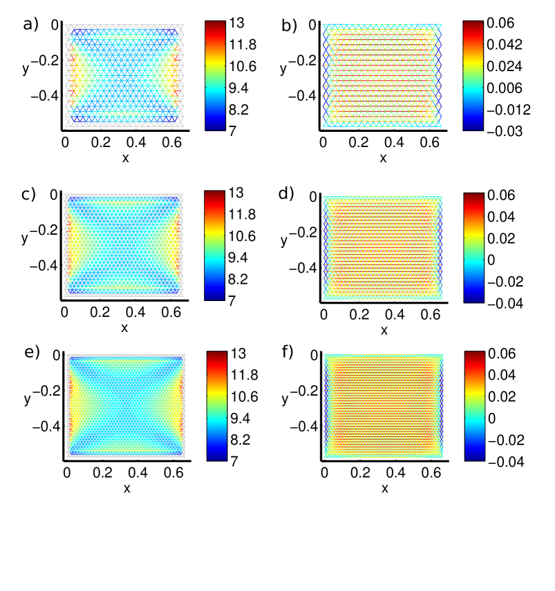
Figure 2: Rectangular bilayer bending with the same parameters as in figure 1 and three values of equilibrium edge length: 1/30 (a,b), 1/45 (c,d) and 1/60 (e,f). Panels a, c, and e show the maximum principal curvatures at the edge midpoints, and panels b, d, and f show the stretching strains in each edge.

In figure 2, we show the results from figure 1c and e together with solutions on two coarser meshes, with equilibrium edge lengths of 1/30 (a,b), 1/45 (c,d), and 1/60 (e,f). Panels a, c, and e compare maximum principal curvatures using the same color scale. Panels b, d, and f compare stretching strains (with nearly the same color scales). The distributions and overall magnitudes of these quantities are quite similar from the finest to the coarsest mesh.

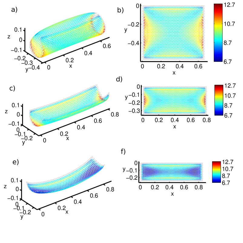
Figure 3: Rectangular bilayer bending with the same parameters as in figure 1 and three initial aspect ratios: (a) Aspect ratio = 1.15 (initial width = 2/3, initial height = $\sqrt{3}/3=0.577$), (b) Aspect ratio = 2.31 (initial width = 0.8, initial height = $\sqrt{3}/5=0.346$) (c) Aspect ratio = 3.46 (initial width = 6/7, initial height = $\sqrt{3}/7=0.247$).

In figure 3, we compare results across three aspect ratios of the initial rectangular shape. All three shapes have maximum curvature along the short direction, although for the largest aspect ratio (panel c) this is difficult to discern since the strip is much shorter in this direction, so it does not show as much overall difference in the $z$ coordinate along this direction. Also, it has larger curvature in the long direction than the shapes in panels a and b. However, for this strip the average curvature along the short direction is 10 times that in the longer direction. The average of the curvature in the short direction decreases from about 9 for the most square shape (a) to about 8 for the most elongated shape (c).

IV General bilayers

We now consider the bending of a set of bilayers with more general planar shapes. Most of the shapes we consider are connected clusters of a small number of equilateral triangles, also called “polyiamonds”, a class of polyforms weisstein1999crc . Such shapes can be represented with equilateral triangular meshes of various levels of refinement, without jagged edges (as occur for the rectangles in figure 3, for example).

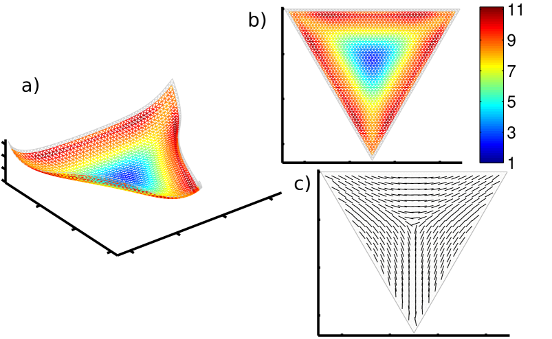
Figure 4: Bending of an equilateral triangular bilayer with the same elastic parameters as in figure 1. The top edge has length 7/9. The values on the color bar indicate the maximum of the principal curvatures at each edge midpoint. a, 3D configuration with coloring given in b, Color map of maximum principal curvatures at each edge midpoint. c, Direction field showing direction of minimum principal curvature at the midpoints of edges.

In figure 4 we show the bending of an equilaterial triangular bilayer with the same elastic parameters as the rectangular bilayer just considered. The maximum curvature, which occurs along the edges, is comparable in magnitude to the maximum curvatures of the rectangles in figure 3, but unlike for the rectangles, here there is a large flattened region at the center. The minimum-curvature direction field (panel c) shows the triangular symmetry of the shape. This equilibrum is not the shape with minimum elastic energy (or global equilibrium), however. Cylindrical bending of the triangle is also an equilbrium, and has smaller total elastic energy.

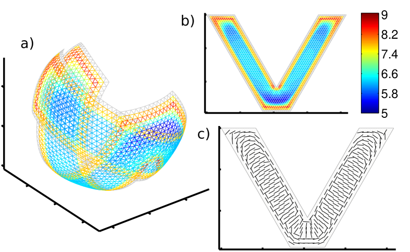
Figure 5: Bending of a V-shaped bilayer with the same elastic parameters as in figure 1. The bottom edge has length 7/9. The values on the color bar indicate the maximum of the principal curvatures at each edge midpoint. a, 3D configuration with coloring given in b, Color map of maximum principal curvatures at each edge midpoint. c, Direction field showing the directions of minimum principal curvature at the midpoints of edges.

Figure 5 shows the bending of a V-shaped bilayer. Here the two arms of the V bend mainly along the longer dimension, in contrast to the rectangular shapes in figure 3, which bend along the shorter dimension. Bending along the longer dimension is also an equilibrium for a rectangle, with slightly lower elastic energy than for bending along the shorter dimension alben2011edge . For the V shape, there is a sharp transition to a region of higher curvature near the boundary, with bending in the opposite direction. The minimum-curvature direction field in panel c shows that near the boundary, there is sharp transition in bending direction. Bending is nearly transverse to the boundary near the edges, and parallel to the boundary further inside.

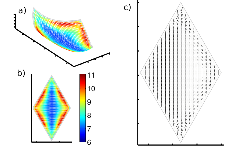
Figure 6: Bending of a bilayer in the shape of a rhombus with the same elastic parameters as in figure 1. The horizontal width is 1/3. The values on the color bar indicate the maximum of the principal curvatures at each edge midpoint. a, 3D configuration with coloring given in b, Color map of maximum principal curvatures at each edge midpoint. c, Direction field showing the directions of minimum principal curvature at the midpoints of edges.

Figure 6 shows the bending of a rhombus. Here the bending is mainly along the shorter dimension, akin to the rectangles of figure 3. The direction of bending does not change except at the farther pair of opposing tips. Near the edges there are regions of increased curvature, larger than those in figure 3.

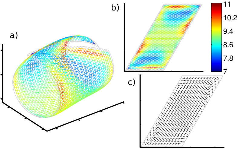
Figure 7: Bending of a tetriamond bilayer with the same elastic parameters as in figure 1. The horizontal width is 1/3. The values on the color bar indicate the maximum of the principal curvatures at each edge midpoint. a, 3D configuration with coloring given in b, Color map of maximum principal curvatures at each edge midpoint. c, Direction field showing the directions of minimum principal curvature at the midpoints of edges.

An oblique strip, a cluster of four equilateral triangles (a tetriamond), is shown in figure 7. The bending is essentially cylindrical, and this time along the longer dimension. The minimum-curvature direction field is almost orthogonal to the longer edges, but there is a noticeable deviation from orthogonality. The curvature is nearly uniform over the middle part of the bilayer, and varies more near the tips with acute angles. The final shape maintains the 180-degree rotational symmetry of the initial shape.

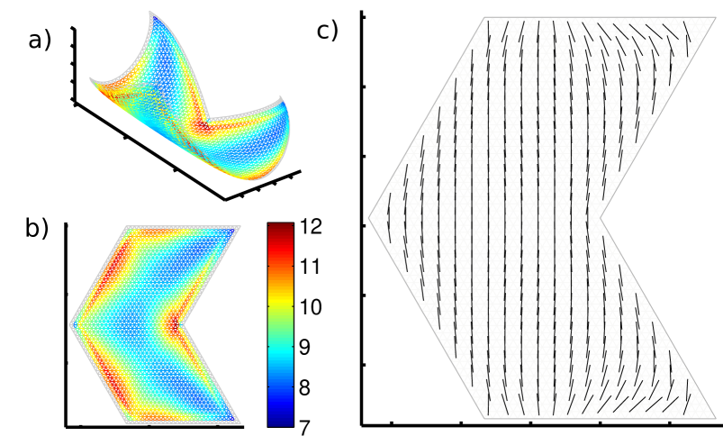
Figure 8: Bending of a tetriamond bilayer with the same elastic parameters as in figure 1. The horizontal width is 1/3. The values on the color bar indicate the maximum of the principal curvatures at each edge midpoint. a, 3D configuration with coloring given in b, Color map of maximum principal curvatures at each edge midpoint. c, Direction field showing the directions of minimum principal curvature at the midpoints of edges.

A different tetriamond is shown in figure 8. The bending is again essentially cylindrical, but this time along the shorter dimension. Now the minimum-curvature direction field is essentially orthogonal to the upper and lower edges, giving a shape with bilateral symmetry.

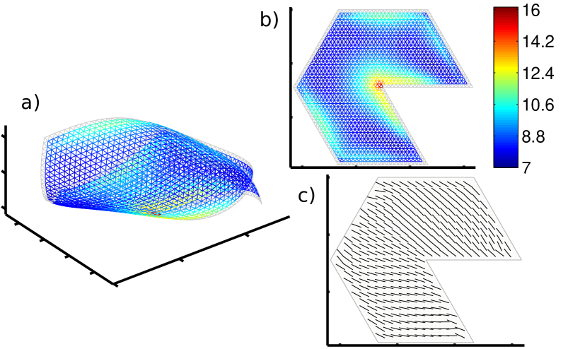
Figure 9: Bending of a pentiamond bilayer with the same elastic parameters as in figure 1. The horizontal width is 1/3. The values on the color bar indicate the maximum of the principal curvatures at each edge midpoint. a, 3D configuration with coloring given in b, Color map of maximum principal curvatures at each edge midpoint. c, Direction field showing the directions of minimum principal curvature at the midpoints of edges.

A pentiamond, or hexagon with a wedge removed, is shown in figure 9. The 3D configuration has a bilateral symmetry inherited from the 2D shape. The bending is not quite cylindrical. The minimum-curvature direction field gradually rotates, moving around the central corner. At the central corner, the curvature is significantly increased, perhaps indicating a smoothed version of a conical singularity.

Figure 10: Bending of a pentiamond bilayer with the same elastic parameters as in figure 1. The top edge has length 1/2. The values on the color bar indicate the maximum of the principal curvatures at each edge midpoint. a, 3D configuration with coloring given in b, Color map of maximum principal curvatures at each edge midpoint. c, Direction field showing the directions of minimum principal curvature at the midpoints of edges.

Figure 10 shows the bending of a different pentiamond. Again, the curvature is largest at the concave angle. The minimum-curvature directions are mainly vertical on the right side of panel c, and transition to an oblique angle on the left side, yielding an approximate partition into two regions of bending. Overall, the bending is mainly along the longest dimension of the shape.

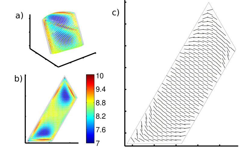
Figure 11: Bending of a pentiamond bilayer with the same elastic parameters as in figure 1. The bottom edge has length 1/4. The values on the color bar indicate the maximum of the principal curvatures at each edge midpoint. a, 3D configuration with coloring given in b, Color map of maximum principal curvatures at each edge midpoint. c, Direction field showing the directions of minimum principal curvature at the midpoints of edges.

A strip-like pentiamond is shown in figure 11, similar to the tetriamond of figure 7. Unlike that shape, here the initial and final shapes have bilateral symmetry. Similarly to the shape of figure 7, the bending is mainly along the longer dimension, and curvature varies most near the two ends.

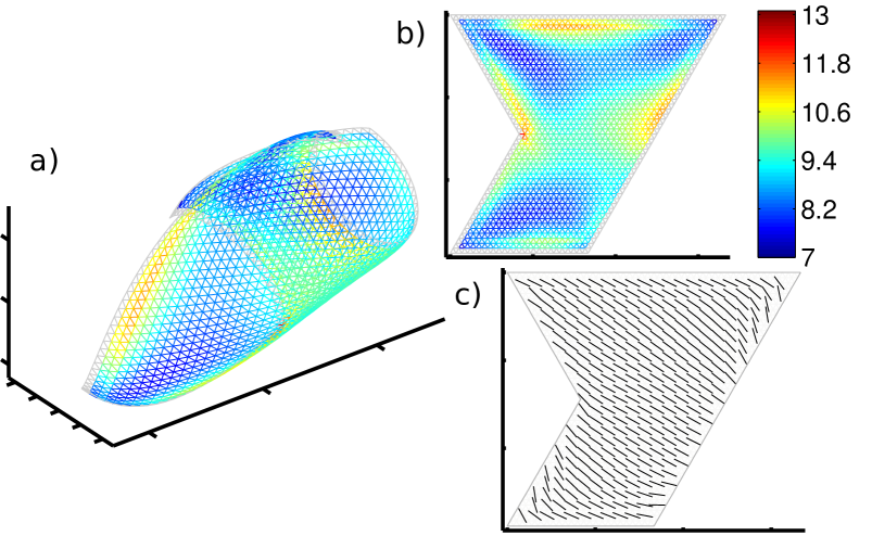
Figure 12: Bending of a pentiamond bilayer with the same elastic parameters as in figure 1. The top edge has length 2/3. The values on the color bar indicate the maximum of the principal curvatures at each edge midpoint. a, 3D configuration with coloring given in b, Color map of maximum principal curvatures at each edge midpoint. c, Direction field showing the directions of minimum principal curvature at the midpoints of edges.

In figure 12, another pentiamond bilayer is shown. The shape has no symmetries, and the overall bending is strip-like, with the minimum-curvature directions mainly orthogonal to the longest linear dimension of the object.

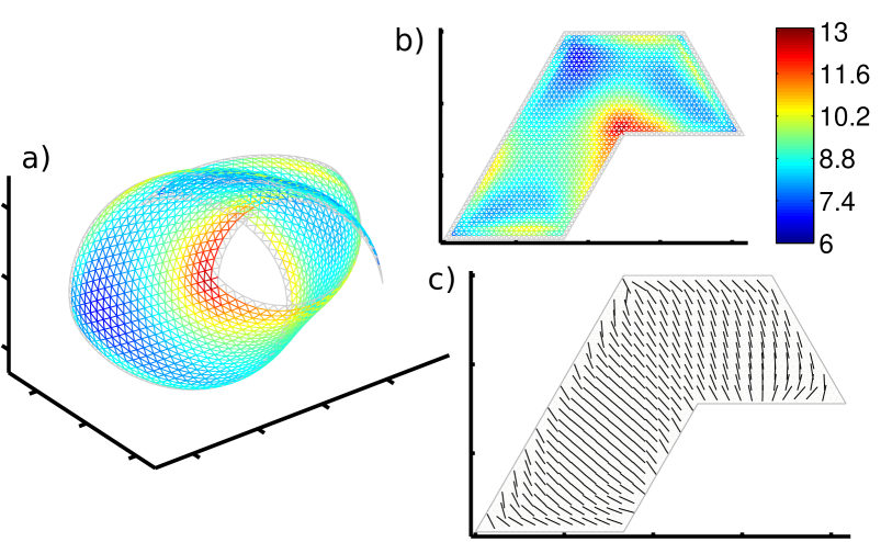
Figure 13: Bending of a pentiamond bilayer with the same elastic parameters as in figure 1. The top edge has length 1/3. The values on the color bar indicate the maximum of the principal curvatures at each edge midpoint. a, 3D configuration with coloring given in b, Color map of maximum principal curvatures at each edge midpoint. c, Direction field showing the directions of minimum principal curvature at the midpoints of edges.

The last of the four pentiamonds is shown in figure 13, another shape without symmetries. The bending is most similar to that of figure 10, with the minimum-curvature direction field again split mainly into two regions, with some amount of convergence at the concave angle. The bending is mainly along the longest dimension.

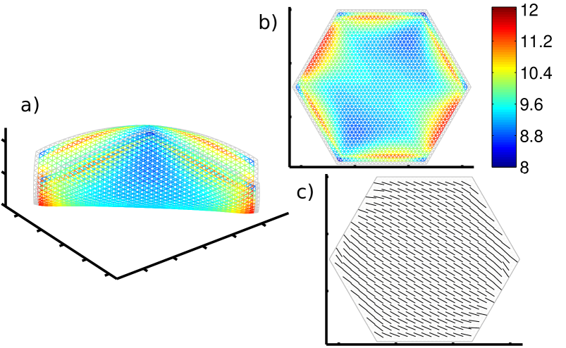
Figure 14: Bending of a hexagonal bilayer with the same elastic parameters as in figure 1. The sides have length 1/3. The values on the color bar indicate the maximum of the principal curvatures at each edge midpoint. a, 3D configuration with coloring given in b, Color map of maximum principal curvatures at each edge midpoint. c, Direction field showing the directions of minimum principal curvature at the midpoints of edges.

We consider only two of the twelve hexiamonds. In figure 14, a hexagonal bilayer is shown. The bending is roughly cylindrical, and nearly along a line connecting two opposite vertices. The curvature distribution has a bilateral symmetry, with the strongest intensification of curvature at the sides parallel to the bending direction.

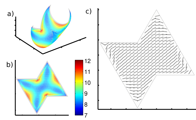
Figure 15: Bending of a hexiamond with the same elastic parameters as in figure 1. The four shorter sides have length 1/3 and the two longer sides have length 2/3. The values on the color bar indicate the maximum of the principal curvatures at each edge midpoint. a, 3D configuration with coloring given in b, Color map of maximum principal curvatures at each edge midpoint. c, Direction field showing the directions of minimum principal curvature at the midpoints of edges.

A second hexiamond, with rotational and reflectional symmetries, is shown in figure 15. The bending is mainly cylindrical here also, but there is a deviation in bending direction near the 60-degree corners, similar to that which has occured in most but not all of the 60-degree corners in the bilayers previously discussed. These corners curl inward toward the center of the shape.

We have presented just a single equilibrium shape for a variety of bilayer shapes, most corresponding to simple polyiamonds. These shapes show how the simple cylindrical bending of figures 1 and 3 are modified for oblique shapes and shapes with different or no symmetries. These examples may be useful test cases from which to abstract the general dependence of bilayer bending on initial shape.

V Conclusion

We have presented a simple discrete formula for the elastic energy of a bilayer, in terms of the geometry of a single mesh representing the central surface of the substrate layer. The formula allows for fast simulations of bending bilayers with general geometries. We have found good agreement between our simulations of a rectangular bilayer, and an approximate analytical solution.

Simulations of a set of shapes composed of clusters of equilateral triangles (polyiamonds) present some generic behaviors of bilayers which may lead to an understanding of the relationship between bending directions and bilayer shapes. Some of the bilayers show cylindrical bending in the same direction over the entire bilayer, and often along either the shortest or longest linear extent of the initial shape. Slight deviations in bending direction occur sometimes but not always near acute-angled corners of the bilayers, where the shape bends inwards towards the center. Larger variations in curvature occur near edges and corners, and the curvature is particularly intensified near obtuse-angled corners, as in the pentiamond which is a hexagon with a sector removed. In this shape and some others, the direction of bending changes gradually, leading to bending which is somewhat conical rather than cylindrical. Some other shapes are nearly partitioned into two regions, with bending along distinct directions in each region.

Because the bilayers are thin, the equilibria are all close to developable surfaces. Unlike thin homogeneous sheets, in bilayers there is always considerable in-plane stretching energy, in the direction of small curvature. The equilibria we have found preserve many of the initial symmetries of the flat bilayer. Performing our simulations with other initial guesses for the equilibria can produce different and possibly less symmetrical equilibria.

Appendix A Extension due to bending

Let us consider a point $\mathbf{X}_{0}$ on the central surface of the substrate. Let the curvature at $\mathbf{X}_{0}$ in a direction $\mathbf{v}$ be $\kappa$, and the radius of curvature be $R=1/\kappa$. Consider the intersection of the surface with the plane spanned by $\mathbf{v}$ and the normal to the surface, $\mathbf{n}$. This is a curved line passing through $\mathbf{X}_{0}$. A short segment of length $l$ near $\mathbf{X}_{0}$ is approximated by an arc of a circle tangent to the surface at $\mathbf{X}_{0}$ with radius $R$. The set of corresponding points on the central surface of the actuated layer is a parallel curve, approximated by a concentric arc with radius $R+h$, and length $l+\delta l$. Because the arcs are concentric,

$$\frac{l+\delta l}{l}=\frac{R+h}{R}\;\;\mbox{and thus}\;\;\frac{\delta l}{l}=h\kappa,$$ (10)

so the strain in the actuated layer is $h\kappa$ plus that in the substrate. Furthermore, the ratio of the curvature of the actuated layer central surface $\kappa_{a}$ to that of the substrate $\kappa$ is

$$\frac{\kappa_{a}}{\kappa}=\frac{R}{R+h}=\frac{1}{1+h\kappa}=1-h\kappa+O\left((h\kappa)^{2}\right).$$ (11)

Appendix B Discrete formula for extension due to bending

In order to derive equation (4), we consider the discretization in the vicinity of a point on the central surface of the substrate, which is assumed to be a smooth surface. Without loss of generality, we can assume that the point is at the origin in $(x,y,z)$, and that, up to quadratic order, the central surface of the subtrate is given by

$$z(x,y)=\frac{1}{2}k_{x}x^{2}+\frac{1}{2}k_{y}y^{2}.$$ (12)

An arbitrary smooth surface can be brought into this form (up to quadratic order), in the vicinity of a point on the surface, by translating the point to the origin and rotating the surface about the point so that the directions of principal curvature lie along the $x$ and $y$ axes.

Figure 16: Schematic diagram of a set of triangles showing the notation used in deriving the formula for the strain in edge ${\tilde{\mathbf{X}}}_{1}$-${\tilde{\mathbf{X}}}_{2}$ due to bending. Here the amount of bending is exaggerated so the differences between vectors are visible.

We now assume that the origin coincides with the midpoint of an edge in our triangulation of the substrate central surface. We determine the stretching of this edge in the actuated layer relative to that in the substrate, under the bending of the substrate given by (12). In figure 16 we show a portion of the triangular mesh consisting of the two triangles which bound the ${\mathbf{X}}_{1}$-${\mathbf{X}}_{2}$ edge, and the four other triangles which share an edge with these triangles. We can approximate the curvatures of the surface simply in terms of the angles between the normals to these triangles. In general the mesh has an arbitrary orientation with respect to the directions of principal curvature (here, the $x$ and $y$ axes). Thus in figure 16 we assume an arbitrary angle $\phi$ between the $x$-axis and the projection of the ${\mathbf{X}}_{1}$-${\mathbf{X}}_{2}$ edge on the $x$-$y$ plane. We first assume that the $x$-$y$ coordinates of the eight points in figure 16 lie on the undeformed equilateral triangular lattice, which is a good approximation for small strains:

$${\mathbf{X}}_{1,x} =\frac{d_{eq}}{2}\cos{\phi},{\mathbf{X}}_{1,y}=\frac{d_{eq}}{2}\sin{\phi},$$ (13)

$$\left({\mathbf{X}}_{2,x},{\mathbf{X}}_{2,y}\right) =-\left({\mathbf{X}}_{1,x},{\mathbf{X}}_{1,y}\right)$$ (14)

$$\left({\mathbf{X}}_{3,x},{\mathbf{X}}_{3,y}\right) =\left({\mathbf{X}}_{1,x},{\mathbf{X}}_{1,y}\right)+d_{eq}\left(\cos{\left(\phi-\frac{\pi}{3}\right)},\sin{\left(\phi-\frac{\pi}{3}\right)}\right)$$ (15)

$$\left({\mathbf{X}}_{4,x},{\mathbf{X}}_{4,y}\right) =\left({\mathbf{X}}_{3,x},{\mathbf{X}}_{3,y}\right)-d_{eq}\left(\cos{\phi},\sin{\phi}\right)$$ (16)

$$\left({\mathbf{X}}_{5,x},{\mathbf{X}}_{5,y}\right) =\left({\mathbf{X}}_{4,x},{\mathbf{X}}_{4,y}\right)-d_{eq}\left(\cos{\phi},\sin{\phi}\right)$$ (17)

$$\left({\mathbf{X}}_{6,x},{\mathbf{X}}_{6,y}\right) =\left({\mathbf{X}}_{1,x},{\mathbf{X}}_{1,y}\right)+d_{eq}\left(\cos{\left(\phi+\frac{\pi}{3}\right)},\sin{\left(\phi+\frac{\pi}{3}\right)}\right)$$ (18)

$$\left({\mathbf{X}}_{7,x},{\mathbf{X}}_{7,y}\right) =\left({\mathbf{X}}_{6,x},{\mathbf{X}}_{6,y}\right)-d_{eq}\left(\cos{\phi},\sin{\phi}\right)$$ (19)

$$\left({\mathbf{X}}_{8,x},{\mathbf{X}}_{8,y}\right) =\left({\mathbf{X}}_{7,x},{\mathbf{X}}_{7,y}\right)-d_{eq}\left(\cos{\phi},\sin{\phi}\right)$$ (20)

The $z$ coordinates of ${\mathbf{X}}_{1}$-${\mathbf{X}}_{8}$ are found by inserting the $x$-$y$ coordinates in (13)-(20) into (12). The points which correspond to ${\mathbf{X}}_{1}$-${\mathbf{X}}_{2}$ in the central surface of the actuated layer are

$${\tilde{\mathbf{X}}}_{1} ={\mathbf{X}}_{1}+h{\mathbf{n}}_{1}$$ (21)

$${\tilde{\mathbf{X}}}_{2} ={\mathbf{X}}_{2}+h{\mathbf{n}}_{2}$$ (22)

where ${\mathbf{n}}_{1}$ and ${\mathbf{n}}_{2}$ are the unit normal vectors to the surface (12) at ${\mathbf{X}}_{1}$ and ${\mathbf{X}}_{2}$, respectively:

$${\mathbf{n}}_{1} =\left(-k_{x}\frac{d_{eq}}{2}\cos{\phi},\,-k_{y}\frac{d_{eq}}{2}\sin{\phi},\,1\right)\left(1+O\left(d_{eq}^{2}\right)\right)$$ (23)

$${\mathbf{n}}_{2} =\left(k_{x}\frac{d_{eq}}{2}\cos{\phi},\,k_{y}\frac{d_{eq}}{2}\sin{\phi},\,1\right)\left(1+O\left(d_{eq}^{2}\right)\right).$$ (24)

We may now determine the length of the edge ${\tilde{\mathbf{X}}}_{1}$-${\tilde{\mathbf{X}}}_{2}$ relative to $d_{eq}$:

$$\left|{\tilde{\mathbf{X}}}_{1}-{\tilde{\mathbf{X}}}_{2}\right|-d_{eq}=-hd_{eq}(k_{x}\cos^{2}\phi+k_{y}\sin^{2}\phi)\left(1+O\left(d_{eq}^{2}\right)\right)\left(1+O\left(h\right)\right).$$ (25)

If the corresponding edge ${\mathbf{X}}_{1}$-${\mathbf{X}}_{2}$ in the substrate has a length $d$ different from $d_{eq}$, then (25) still holds but with $d$ in place of $d_{eq}$. Thus it gives the difference in stretching between the actuated layer central surface and the substrate at corresponding edges.

We now show that (25) is approximately $-h\sqrt{3}$ times the average of the angles between the normals to the four triangles adjacent to the two triangles which share the ${\mathbf{X}}_{1}$-${\mathbf{X}}_{2}$ edge. We define vectors normal to triangles 1-6

$${\mathbf{n}}^{1} =({\mathbf{X}}_{1}-{\mathbf{X}}_{3})\times({\mathbf{X}}_{4}-{\mathbf{X}}_{3})$$ (26)

$${\mathbf{n}}^{2} =({\mathbf{X}}_{4}-{\mathbf{X}}_{2})\times({\mathbf{X}}_{2}-{\mathbf{X}}_{1})$$ (27)

$${\mathbf{n}}^{3} =({\mathbf{X}}_{4}-{\mathbf{X}}_{5})\times({\mathbf{X}}_{2}-{\mathbf{X}}_{5})$$ (28)

$${\mathbf{n}}^{4} =({\mathbf{X}}_{7}-{\mathbf{X}}_{6})\times({\mathbf{X}}_{1}-{\mathbf{X}}_{6})$$ (29)

$${\mathbf{n}}^{5} =({\mathbf{X}}_{7}-{\mathbf{X}}_{1})\times({\mathbf{X}}_{2}-{\mathbf{X}}_{1})$$ (30)

$${\mathbf{n}}^{6} =({\mathbf{X}}_{7}-{\mathbf{X}}_{2})\times({\mathbf{X}}_{8}-{\mathbf{X}}_{2})$$ (31)

The angle between ${\mathbf{n}}^{1}$ and ${\mathbf{n}}^{2}$ is

$$\varphi_{1}=\mbox{Arccos}\left(\frac{{\mathbf{n}}^{1}\cdot{\mathbf{n}}^{2}}{\|{\mathbf{n}}^{1}\|\|{\mathbf{n}}^{2}\|}\right)$$ (32)

Using (26,27) we define a function $a_{1}$ by

$$\frac{4}{3}{\mathbf{n}}^{1}\cdot{\mathbf{n}}^{2}=d_{eq}^{4}(1+d_{eq}^{2}a_{1}(k_{x},k_{y},\phi)),$$ (33)

$a_{1}$ has terms which are quadratic in $k_{x}$ and $k_{y}$ and include trigonometric functions of $\phi$. We also define $b_{1}$ and $c_{1}$ for terms in the denominator of (32):

$$\frac{4}{3}\|{\mathbf{n}}^{1}\|^{2} =d_{eq}^{4}(1+d_{eq}^{2}b_{1}(k_{x},k_{y},\phi))$$ (34)

$$\frac{4}{3}\|{\mathbf{n}}^{2}\|^{2} =d_{eq}^{4}(1+d_{eq}^{2}c_{1}(k_{x},k_{y},\phi))$$ (35)

Thus

$$\frac{{\mathbf{n}}^{1}\cdot{\mathbf{n}}^{2}}{\|{\mathbf{n}}^{1}\|\|{\mathbf{n}}^{2}\|}=1+d_{eq}^{2}\left(a_{1}-\frac{b_{1}}{2}-\frac{c_{1}}{2}\right)\left(1+O\left(d_{eq}^{2}\right)\right).$$ (36)

We define $a_{2}$ and $b_{2}$ in terms of ${\mathbf{n}}^{2}$ and ${\mathbf{n}}^{3}$:

$$\frac{4}{3}{\mathbf{n}}^{3}\cdot{\mathbf{n}}^{2} =d_{eq}^{4}(1+d_{eq}^{2}a_{2}(k_{x},k_{y},\phi))$$ (37)

$$\frac{4}{3}\|{\mathbf{n}}^{3}\|^{2} =d_{eq}^{4}(1+d_{eq}^{2}b_{2}(k_{x},k_{y},\phi))$$ (38)

The angle between ${\mathbf{n}}^{2}$ and ${\mathbf{n}}^{3}$ is

$$\varphi_{2}=\mbox{Arccos}\left(\frac{{\mathbf{n}}^{2}\cdot{\mathbf{n}}^{3}}{\|{\mathbf{n}}^{2}\|\|{\mathbf{n}}^{3}\|}\right)$$ (39)

We expand Arccos in a Taylor series

$$\mbox{Arccos}(1-x)=\sqrt{2x}+O(x^{3/2}).$$ (40)

Thus

$$\frac{1}{2}(\varphi_{1}+\varphi_{2})=\frac{1}{\sqrt{2}}d_{eq}\left(\sqrt{-a_{1}+\frac{b_{1}+c_{1}}{2}}+\sqrt{-a_{2}+\frac{b_{2}+c_{1}}{2}}\right)\left(1+O\left(d_{eq}^{2}\right)\right)$$ (41)

Using trigonometric identities one can show that

$$\frac{1}{\sqrt{2}}\left(\sqrt{-a_{1}+\frac{b_{1}+c_{1}}{2}}+\sqrt{-a_{2}+\frac{b_{2}+c_{1}}{2}}\right)=\frac{1}{\sqrt{3}}\left(k_{x}\cos^{2}\phi+k_{y}\sin^{2}\phi\right).$$ (42)

Therefore by (25),

$$-h\sqrt{3}\,\frac{\varphi_{1}+\varphi_{2}}{2}\left(1+O\left(d_{eq}^{2}\right)\right)\left(1+O\left(h\right)\right)=\left|{\tilde{\mathbf{X}}}_{1}-{\tilde{\mathbf{X}}}_{2}\right|-d_{eq}.$$ (43)

A more symmetrical formula is obtained by using the angles

$$\varphi_{3}=\mbox{Arccos}\left(\frac{{\mathbf{n}}^{4}\cdot{\mathbf{n}}^{5}}{\|{\mathbf{n}}^{4}\|\|{\mathbf{n}}^{5}\|}\right);\quad\varphi_{4}=\mbox{Arccos}\left(\frac{{\mathbf{n}}^{5}\cdot{\mathbf{n}}^{6}}{\|{\mathbf{n}}^{5}\|\|{\mathbf{n}}^{6}\|}\right)$$ (44)

By symmetries of the lattice (13)-(20) and the quadratic surface, $\varphi_{3}=\varphi_{2}$ and $\varphi_{4}=\varphi_{1}$. Thus a more symmetrical alternative to (43) is

$$-h\sqrt{3}\,\frac{\varphi_{1}+\varphi_{2}+\varphi_{3}+\varphi_{4}}{4}\left(1+O\left(d_{eq}^{2}\right)\right)\left(1+O\left(h\right)\right)=\left|{\tilde{\mathbf{X}}}_{1}-{\tilde{\mathbf{X}}}_{2}\right|-d_{eq}.$$ (45)

(45) is more accurate than (43) for surface approximations which are of higher than quadratic order, in which case the principal curvatures have a nonzero gradient at the origin.

Let us now assume that the substrate central surface is strained from the undeformed triangular mesh, given by (13)-(20), with a nonzero in-plane strain tensor $\alpha_{ij}$. The derivation leading to (45) can be repeated, but now there is an additional factor of $1+O(\|\alpha\|)$ multiplying the left side of (45). This error is of the same order as errors already present in the single-plate model represented by (1) and (2) alone. These errors are due to the use of only the linear part of the strain tensor in infinitessimal strain theory, and also due to the discrete approximation (1) (see Seung:1988 ).

Appendix C Estimate of principal curvatures at a point

We now use the framework from appendix B to obtain a discrete estimate for the principal curvatures at the midpoint of an edge in our mesh. We consider the edge shown in figure 16, oriented at an angle $\phi$ with respect to the $x$ axis, and $\pi/2-\phi$ with respect to the $y$ axis. The $x$ and $y$ axes are again assumed to be the directions of principal curvatures, and near the edge midpoint the surface is (12). We can use (45) to estimate the curvature $k_{1}$ in the direction of the edge ${\mathbf{X}}_{1}$-${\mathbf{X}}_{2}$ (i.e. along the angle $\phi$ in figure 16):

$$hk_{1}d_{eq}\approx\frac{\varphi_{1}+\varphi_{2}+\varphi_{3}+\varphi_{4}}{4}.$$ (46)

We can similarly estimate the curvatures along the directions $\phi\pm\pi/3$. Let $k_{2}$ denote the curvature in the direction $\phi+\pi/3$, at the midpoint of ${\mathbf{X}}_{1}$-${\mathbf{X}}_{2}$. We apply formula (46) to the edges ${\mathbf{X}}_{2}$-${\mathbf{X}}_{7}$ and ${\mathbf{X}}_{1}$-${\mathbf{X}}_{4}$ which have angle $\phi+\pi/3$, and take the average as an estimate of the curvature at the midpoint of ${\mathbf{X}}_{1}$-${\mathbf{X}}_{2}$. We take the average of (46) applied to the edges ${\mathbf{X}}_{1}$-${\mathbf{X}}_{7}$ and ${\mathbf{X}}_{2}$-${\mathbf{X}}_{4}$ to estimate $k_{3}$, the curvature in direction $\phi-\pi/3$.

The curvatures $k_{1}$-$k_{3}$ are related to the principal curvatures $k_{x}$ and $k_{y}$ by

$$k_{1} =k_{x}\cos^{2}\phi+k_{y}\sin^{2}\phi.$$ (47)

$$k_{2} =k_{x}\cos^{2}\left(\phi+\frac{\pi}{3}\right)+k_{y}\sin^{2}\left(\phi+\frac{\pi}{3}\right).$$ (48)

$$k_{3} =k_{x}\cos^{2}\left(\phi-\frac{\pi}{3}\right)+k_{y}\sin^{2}\left(\phi-\frac{\pi}{3}\right).$$ (49)

Given our estimates of $k_{1}$-$k_{3}$ at the midpoint of a given edge, we regard (47)-(49) as a system of three nonlinear equations to be solved for three unknowns: the principal curvatures $k_{x}$ and $k_{y}$, and the angle $\phi$ which orients the mesh with respect to the directions of principal curvature. The equations are simpler in terms of the alternate set of three variables

$$\{k_{y},u,A\},\quad u=\cos^{2}\phi,\quad A=k_{x}-k_{y}.$$ (50)

The solutions are

$$u =\frac{1}{2}+\frac{(2k_{1}-k_{2}-k_{3})\,\mbox{sign}(k_{2}-k_{3})}{2\sqrt{3(k_{3}-k_{2})^{2}+(2k_{1}-k_{2}-k_{3})^{2}}},\quad A=\frac{k_{2}-k_{3}}{\sqrt{3u(1-u)}},\quad k_{y}=k_{1}-Au.$$ (51)

Using (51) and (47)-(49) we can estimate the principal curvatures at the midpoints of all the edges in our mesh except those near the boundary, for which not all the edges needed to estimate $k_{1}$, $k_{2}$, and $k_{3}$ exist.

References

- [1] S. Timoshenko et al. Analysis of bi-metal thermostats. J. Opt. Soc. Am, 11(3):233–255, 1925.
- [2] E. Smela, O. Inganäs, Q. Pei, and I. Lundström. Electrochemical muscles: micromachining fingers and corkscrews. Advanced Materials, 5(9):630–632, 1993.
- [3] E. Smela, O. Inganas, and I. Lundstrom. Controlled folding of micrometer-size structures. Science, 268(5218):1735–1738, 1995.
- [4] T.G. Leong, B.R. Benson, E.K. Call, and D.H. Gracias. Thin film stress driven self-folding of microstructured containers. small, 4(10):1605–1609, 2008.
- [5] E. Smela. Conjugated polymer actuators for biomedical applications. Advanced Materials, 15(6):481–494, 2003.
- [6] R. Guerre, U. Drechsler, D. Bhattacharyya, P. Rantakari, R. Stutz, R.V. Wright, Z.D. Milosavljevic, T. Vaha-Heikkila, P.B. Kirby, and M. Despont. Wafer-level transfer technologies for pzt-based rf mems switches. Microelectromechanical Systems, Journal of, 19(3):548–560, 2010.
- [7] E. Sharon, B. Roman, and H.L. Swinney. Geometrically driven wrinkling observed in free plastic sheets and leaves. Physical Review E, 75(4):046211, 2007.
- [8] J. Huang, B. Davidovitch, C.D. Santangelo, T.P. Russell, and N. Menon. Smooth cascade of wrinkles at the edge of a floating elastic film. Physical review letters, 105(3):38302, 2010.
- [9] Y. Klein, E. Efrati, and E. Sharon. Shaping of elastic sheets by prescription of non-euclidean metrics. Science, 315(5815):1116, 2007.
- [10] S. Armon, E. Efrati, R. Kupferman, and E. Sharon. Geometry and mechanics in the opening of chiral seed pods. Science, 333(6050):1726–1730, 2011.
- [11] HS Seung and DR Nelson. Defects in flexible membranes with crystalline order. Phys. Rev. A, 38(2):1005 – 1018, 1988.
- [12] AE Lobkovsky and TA Witten. Properties of ridges in elastic membranes. Phys. Rev. E, 55(2):1577 – 1589, 1997.
- [13] S. Alben and M.P. Brenner. Self-assembly of flat sheets into closed surfaces. Physical Review E, 75(5):056113, 2007.
- [14] E. Katifori, S. Alben, E. Cerda, DR Nelson, and J. Dumais. Foldable structures and the natural design of pollen grains. Proceedings of the National Academy of Sciences of the United States of America, 107(17):7635, 2010.
- [15] ED Landau and EM Lifshitz. Theory of Elasticity. Pergamon Press, 1986.
- [16] M. Christophersen, B. Shapiro, and E. Smela. Characterization and modeling of ppy bilayer microactuators:: Part 1. curvature. Sensors and Actuators B: Chemical, 115(2):596–609, 2006.
- [17] S. Alben, B. Balakrisnan, and E. Smela. Edge effects determine the direction of bilayer bending. Nano Letters, 11:2280–2285, 2011.
- [18] D.J. Struik. Lectures on classical differential geometry. Dover Publications, 1988.
- [19] E.W. Weisstein. CRC Concise Encyclopedia of Mathematics, 1999.