Large Scale Azimuthal Structures Of Turbulence In Accretion Disks
Dynamo triggered variability of accretion.

Abstract

We investigate the significance of large scale azimuthal, magnetic and velocity modes for the MRI turbulence in accretion disks. We perform 3D global ideal MHD simulations of global stratified proto-planetary disk models. Our domains span azimuthal angles of $\pi/4$, $\pi/2$, $\pi$ and $2\pi$. We observe up to $100\%$ stronger magnetic fields and stronger turbulence for the restricted azimuthal domain models $\pi/2$ and $\pi/4$ compared to the full $2\pi$ model. We show that for those models, the Maxwell Stress is larger due to strong axisymmetric magnetic fields, generated by the $\alpha\Omega$ dynamo. Large radial extended axisymmetric toroidal fields trigger temporal magnification of accretion stress. All models display a positive dynamo-$\alpha$ in the northern hemisphere (upper disk). The parity is distinct in each model and changes on timescales of 40 local orbits. In model $2\pi$, the toroidal field is mostly antisymmetric in respect to the midplane. The eddies of the MRI turbulence are highly anisotropic. The major wavelengths of the turbulent velocity and magnetic fields are between one and two disk scale heights. At the midplane, we find magnetic tilt angles around $8-9^{\circ}$ increasing up to $12-13^{\circ}$ in the corona. We conclude that an azimuthal extent of $\pi$ is sufficient to reproduce most turbulent properties in 3D global stratified simulations of magnetised accretion disks.

1 Introduction

Magneto-rotational instability (MRI) can generate MHD turbulence with an outward directed angular momentum transport driving accretion onto the central object (Balbus & Hawley, 1991; Hawley & Balbus, 1991; Balbus & Hawley, 1998). A necessary condition is a good coupling between the gas and magnetic fields, e.g. a well-ionized gas. In proto-planetary disks, dust particles and low temperatures will reduce the ionisation level and therefor the MRI activity (Sano et al., 2000; Fleming & Stone, 2003; Inutsuka & Sano, 2005; Wardle, 2007; Dzyurkevich et al., 2010; Turner et al., 2010). Nevertheless, there are well-ionized regions with possible MRI activity, like the coronal region or the inner or outer disk. The inner disk will be thermally ionized for temperatures greater then $1000K$ (Umebayashi, 1983). The outer disk will be ionized by Cosmic Rays for surface density values below $96g/cm^{2}$ (Umebayashi & Nakano, 2009). In our work we concentrate on well ionized disk regions. To model the evolution of proto-planetary disks and especially to describe the process of planet formation, we need to know detailed informations about the strength of the turbulence. Several processes, like the MHD dynamo or the toroidal field MRI, influence the turbulence level. The evolution of the magnetic and velocities fields at different scales has to be investigated.

In the last decades, a large amount of local-box simulations have been performed to study the small scale MRI turbulence (Brandenburg et al., 1995; Hawley et al., 1995, 1996; Matsumoto & Tajima, 1995; Stone et al., 1996). The MRI works for both, vertical or toroidal seed magnetic fields (Balbus & Hawley, 1991). The MRI launched with initial toroidal field was analyzed through linear calculations (Hawley & Balbus, 1992; Foglizzo & Tagger, 1995; Terquem & Papaloizou, 1996; Papaloizou & Terquem, 1997) and in Taylor-Couette experiments (Gellert et al., 2007; Rüdiger et al., 2007). This experiments showed that most of the energy will be transported to the $m=1$ mode. A similar inverse energy cascade was found in local box simulations as well (Johansen et al., 2009). Here the turbulent advection term in the induction equation drives large-scale radial magnetic field.

The locality and anisotropy of the MRI turbulence is an important aspect for dust growth and therefor the planet formation. The eddies are stretched in the azimuthal direction due to the strong shear. They have a characteristic low tilt angle in the $r-\phi$ plane (Guan et al., 2009). Several works confirmed this tilt angle for the velocity and the magnetic fields (Guan et al., 2009; Fromang, 2010; Davis et al., 2010; Guan & Gammie, 2011; Sorathia et al., 2011). The size of the corresponding correlation wavelengths is dependent on resolution (Guan et al., 2009) and converges by using a fixed value of viscous and explicit dissipation in unstratified local simulations (Fromang, 2010). Unstratified global models interpret the magnetic tilt angle as convergence parameter (Sorathia et al., 2011). They found convergence with tilt angles around $13^{\circ}$. Beckwith et al. (2011) found tilt angles of $9^{\circ}$ in global stratified simulations with spatial structures of the turbulent field in the order of H.

Global disk simulations (Armitage, 1998; Hawley, 2000; Arlt & Rüdiger, 2001; Fromang & Nelson, 2006, 2009; Dzyurkevich et al., 2010; Flock et al., 2011; Beckwith et al., 2011; Sorathia et al., 2011) are used to study the MRI evolution on large scales. Beckwith et al. (2011) found a stronger accretion stress compared to Fromang & Nelson (2006) and Flock et al. (2011) with a stronger initial toroidal field. Unstratified simulations show a similar correlation between accretion stress and the initial plasma beta (Hawley et al., 1995). Here a stronger seed field will drive to stronger accretion stress. The majority of stratified global disk simulations has been done for restricted ($\phi\leq\pi/2$) azimuthal domain sizes. At first glance, MRI turbulence behaves similar for both full $2\pi$ and smaller domain sizes (Hawley, 2000).

In our previous work we compared stratified simulations of $\pi/4$ and $2\pi$ in azimuth. There, we observe stronger azimuthal fields for the $\pi/4$ domain size (Flock et al., 2011). Recent unstratified global simulations (Sorathia et al., 2011) do not show large differences between domain size of $\pi/4$ and $2\pi$. This fact indicates a mean field dynamo mechanism. The stratification is crucial for driving $\alpha\Omega$ dynamo in disks and therefor for the creation of large scale magnetic fields (Krause & Raedler, 1980). With this work we perform a detailed study of different azimuthal domain sizes. We investigate the turbulent and the mean field evolution for the velocity and magnetic fields.

In stratified disk simulations, there is a periodic change of sign for the mean toroidal magnetic field. A similar periodicity of toroidal magnetic field, known as butterfly diagram, is observed in the sun. It could be explained by a MHD dynamo process. The MRI could be self-sustaining by a analogous dynamo process (Hawley et al., 1996; Lesur & Ogilvie, 2008b, a; Gressel, 2010; Simon et al., 2011). Strong shear in accretion disks will wind up any radial magnetic field generated by MRI and produce toroidal field. This field will act as seed for the MRI again. Solutions for $\alpha\Omega$ dynamos in rotating systems were presented by Ruediger & Kichatinov (1993); Elstner et al. (1996). Calculations of the dynamo-$\alpha$ for MRI have been performed in local box simulations Brandenburg et al. (1995); Brandenburg & Donner (1997); Rekowski et al. (2000); Ziegler & Rüdiger (2000); Davis et al. (2010); Gressel (2010) showing a negative dynamo-$\alpha$. Brandenburg & Donner (1997); Rüdiger & Pipin (2000) explained the negative sign as an effect of vertical buoyancy. The first indications for a positive dynamo-$\alpha$ were found in global disk simulations (Arlt & Rüdiger, 2001; Arlt & Brandenburg, 2001). Dynamo solutions for positive or negative dynamo-$\alpha$ predict long-term global mean magnetic fields which become symmetric (quadrupole, dynamo-$\alpha^{north}<0$ ) or asymmetric (dipole, dynamo-$\alpha^{north}>0$). E.g. dipole solutions support the creation of disk wind and jets (Rekowski et al., 2000). A review of dynamo action in accretion disks was presented by Brandenburg & Subramanian (2005); Brandenburg & von Rekowski (2007); Blackman (2010).
The connection between the dynamo processes and the large-scale magnetic field oscillations was shown by Lesur & Ogilvie (2008b); Gressel (2010); Simon et al. (2011). These oscillations are universal for stratified MRI simulations (Stone et al., 1996; Miller & Stone, 2000) with timescales of ten local orbits, presented recently in local (Gressel, 2010; Simon et al., 2011; Hawley et al., 2011; Guan & Gammie, 2011) and global (Sorathia et al., 2010; Dzyurkevich et al., 2010; Flock et al., 2011; Beckwith et al., 2011) simulations. We use the second order Godunov code PLUTO which was successfully applied in recent global simulations (Flock et al., 2010, 2011; Uribe et al., 2011; Beckwith et al., 2011). The paper is structured in the following way:
First, we describe the disk model and the numerical parameter. For the results in section 3 we study the turbulent and the mean field evolution for all azimuthal domain. Section 4 and 5 present discussion and summary.

2 Setup

Our disk model is presented in detail in Flock et al. (2011). We give here a summary of our physical and numerical initial conditions.

Disk model

The HD initial conditions of density, pressure and azimuthal velocity follow a hydrostatic equilibrium. We set

$$\rho=\rho_{0} R^{-3/2}\exp{}\Bigg{(}\frac{\sin{(\theta)}-1}{(H/R)^{2}}\Bigg{)}$$

with $\rho_{0}=1.0$, $\rm H/R=c_{0}=0.07$, $R=r\sin{(\theta)}$. The pressure follows locally an isothermal equation of state: $P=c_{s}^{2}\rho$ with $\rm c_{s}=c_{0}/\sqrt{R}$. The azimuthal velocity is set to

$$V_{\phi}=\sqrt{\frac{1}{r}}\Bigg{(}1-\frac{2.5}{\sin(\theta)}c^{2}_{0}\Bigg{)}.$$

The initial velocities $V_{r}$ and $V_{\theta}$ are set to a white noise perturbation amplitude of $V_{r,\theta}^{Init}=10^{-4}c_{s}$. We start the simulation with a pure toroidal magnetic seed field with constant plasma beta $\beta=2P/B^{2}=25$.
The radial domain extends from 1 to 10 AU. The $\theta$ domain covers $\pm$ 4.3 disk scale heights, or $\theta=\pi/2\pm 0.3$. For the azimuthal domain we use four different models: $\phi^{extent}=\pi/4$, $\pi/2$, $\pi$ and $2\pi$. We use a uniform grid in spherical coordinates with an aspect ratio at 5 AU of $1:0.67:1.74$ $(\Delta r:r\Delta\theta:r\Delta\phi\sin{\theta})$. The resolution is fixed to $N_{r}:384$, $N_{\theta}=192$ , $N_{\phi}=768\cdot\phi_{extent}/(2\pi)$. We have around 23 grid cells per pressure scale height.
Buffer zones extent from 1 to 2 AU as well as from 9 to 10 AU. In the buffer zones we use a linearly increasing resistivity to the boundary. This damps the magnetic field fluctuations and suppresses boundary interactions. In the buffer zones we use also a relaxation function which reestablishes gently the initial value of density over a time period of one local orbit. In the buffer zones we set: $\rm\rho^{new}=\rho-(\rho-\rho^{\rm Init})\cdot\Delta t/T_{Orbits}$. Our outflow boundary condition projects the radial gradients in density, pressure and azimuthal velocity into the radial boundary and the vertical gradients in density and pressure at the $\theta$ boundary. We ensure to have no inflow velocities. For an inward pointing velocity we mirror the values in the ghost cell to ensure no inward mass flux. The $\theta$ boundary condition for the magnetic field are set to zero gradient, which approximates ”force-free” - outflow conditions. The normal component of the magnetic field in the ghost cells is always set to have $\nabla\cdot\vec{B}$ = 0.

Numerical setup

The detailed numerical configuration is presented in Flock et al. (2010) and was also successfully used in recent global simulations by Beckwith et al. (2011). For all runs we employ the second order scheme in PLUTO with the HLLD Riemann solver (Miyoshi & Kusano, 2005), piece-wise linear reconstruction and $2^{nd}$ order Runge Kutta time integration. We treat the induction equation with the ”Constrained Transport” (CT) method in combination with the upwind CT method described in Gardiner & Stone (2005). All models were performed on a Blue-gene/P cluster for in total over 3 million CPU hours.

2.1 Measurement and integration

For our analysis we use the central domain from 3 to 8 AU. Total volume integrations or a variable $F$, as used for the total stress are performed with

$$F^{total}=\int FdV=\int_{3}^{8}\int_{\theta_{begin}}^{\theta_{end}}\int_{0}^{\phi^{extent}}Fr^{2}\sin{\theta}drd\theta d\phi.$$

In global disk models, the gas dynamics are only self-similar along the azimuth. Therefor, mean values like $\overline{v_{\phi}}$, are always averaged over azimuth. This includes the calculation of the turbulent $EMF^{\prime}$ in Fig. 11. For further analysis we always use an 2D dataset of mean values, e.g. $\overline{v_{\phi}}(r,\theta)$ to construct the 3D turbulent dataset $v^{\prime}_{\phi}(r,\theta,\phi)=v_{\phi}(r,\theta,\phi)-\overline{v_{\phi}}(r,\theta)$. For volume integration over mean values, as $\alpha_{SS}^{mean}$, we use

$$\int dV=\int_{3}^{8}\int_{\theta_{beg}}^{\theta_{begin}}r^{2}\sin{\theta}drd\theta.$$

Some results are determined in the center of computational domain. Analysis done at 4.5 AU are the tilt angle calculations, Fig. 6, the mean field contour plots, Fig. 9, the parity, Fig. 10, the dynamo coefficients in Fig. 11. This results are averaged over azimuth and a small radial extent ($\pm 0.5$ H = 0.16 AU). For the time evolution of the tilt angle, Fig. 6, top, we average vertically $\pm 0.5H$ at the midplane. Radial contour plots are averaged over azimuth and height, between $\rm 0-1.5H$. This applies for the mean toroidal field Fig. 3, the dynamo Fig. 11 and the mean fields in Fig. 12. The parity is averaged over the total disk height at 4.5 AU, Fig. 10.

3 Results

In this section we investigate the turbulent and mean field evolution for the azimuthal MRI for different azimuthal domain sizes. Table 1 summarises the results of accretion stress, contribution of mean magnetic field to the total stress, dynamo-$\alpha$ and RMS velocities for all models. Table 2 summarises results of the two-point correlation function, including tilt angles, major and minor wavelength. For all models, the accretion disk becomes unstable to MRI on timescales of ten local orbits. All models develop an oscillating zero-net flux configuration after around 250 inner orbits.

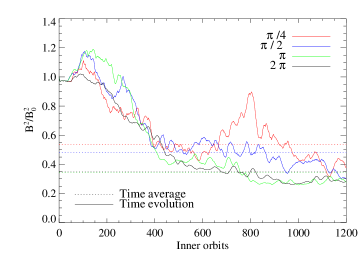
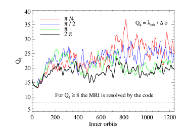
Figure 1: Left: Total magnetic energy evolution over time. Right: Toroidal quality factor $Q_{\phi}$ over time. All models show a well resolved MRI.

The time evolution of total magnetic energy, Fig. 1 left, is normalised over the total initial magnetic field energy $B_{0}^{2}$. It shows the peak of magnetic energy shortly after the linear MRI phase around 100 inner orbits. Between 100 and 400 years, the total magnetic energy decreases due to loss of the net magnetic flux and mass loss (see also Fig. 13 in Flock et al. (2011) and Fig. 3 in Beckwith et al. (2011)). After 400 years, $\pi/4$ and $\pi/2$ models show strong fluctuations while $\pi$ and $2\pi$ models do saturate. In the saturated state ($\gtrsim$ 800 inner orbits), the total magnetic energy evolution shows a relative constant level for the $\pi$ and $2\pi$ model.
All models have the same resolution per $\phi$ extent ($\phi^{\rm extent}/N_{\phi}$). The toroidal quality factor $Q_{\phi}=\lambda_{crit}/\Delta\phi$ shows the quality of resolved MRI ($Q_{\phi}\geq 8$). We follow the analysis done by (Noble et al., 2010; Sorathia et al., 2011) and calculate the mean $Q_{\phi}$ for the central domain (3 to 8 AU). The definition is similar to the toroidal quality factor $Q_{\phi}$ by Hawley et al. (2011).

$$\frac{\lambda_{crit}^{B_{\phi}}}{\Delta\phi}=2\pi\sqrt{\frac{16}{15}\frac{2}{\beta_{\phi}^{B_{\phi}}}}\frac{c_{0}}{\Delta\phi}=2\pi\sqrt{\frac{16}{15}}\frac{|B_{\phi}|\cdot r}{\sqrt{\rho}\Omega\Delta\phi}$$

Fig. 1, right, shows $Q_{\phi}$ over time. For all models we have $Q_{\phi}>8$. The $\pi/4$ and $\pi/2$ show a higher $Q_{\phi}$ due to stronger magnetic fields.

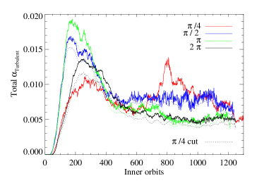
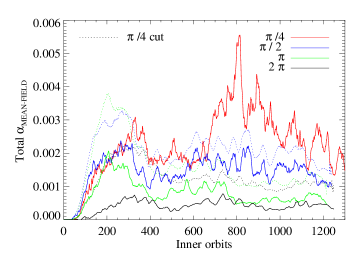
Figure 2: Left: Volume integrated $\alpha_{SS}$ value for all models. Right: Volume integrated $\alpha_{SS}$ values using only the Maxwell component with the mean magnetic fields. Dotted lines show same results but for a $\pi/4$ average ($0-\pi/4$) instead of whole domain size.

3.1 Turbulent evolution - $\alpha$ value

We start the comparison with the volume integrated turbulent stress scaled on the local pressure, e.g. the Shakura-Sunyaev $\alpha_{SS}$. The $\alpha_{SS}$ value is determined from the turbulent Reynolds stress $\rm T_{R}=\overline{\rho v^{\prime}_{\phi}v^{\prime}_{R}}$ and Maxwell stress $\rm T_{M}=\overline{B_{\phi}B_{R}}/4\pi$. We split the total $\alpha_{\rm SS}$ into a mean and turbulent component. For the Maxwell stress, we split the magnetic field components into the turbulent and mean component, e.g. $\rm B_{\phi}=B^{\prime}_{\phi}+\overline{B_{\phi}}$. This leads to a second Maxwell stress component, e.g. the mean Maxwell stress $\rm T^{mean}_{M}=\overline{B_{\phi}}\cdot\overline{B_{R}}/4\pi$. For the volume integrated turbulent $\rm\alpha_{SS}^{turb}$ value we integrate the mass weighted stresses over the central domain

$$\rm\alpha_{SS}^{turb}=\frac{\int\rho\Bigg{(}\frac{v^{\prime}_{\phi}v^{\prime}_{R}}{c^{2}_{s}}-\frac{B^{\prime}_{\phi}B^{\prime}_{R}}{4\pi\rho c^{2}_{s}}\Bigg{)}dV}{\int\rho dV}.$$

The same is done for the mean Maxwell stress

$$\rm\alpha_{SS}^{mean}=\frac{\int\overline{\rho}\Bigg{(}-\frac{\overline{B_{\phi}}\cdot\overline{B_{R}}}{4\pi\overline{\rho}\overline{c^{2}_{s}}}\Bigg{)}dV}{\int\overline{\rho}dV}.$$

The volume integrated $\rm\alpha_{SS}^{turb}$ (Fig. 2 left - solid line) and the volume integrated $\rm\alpha_{SS}^{mean}$ (Fig. 2 right - solid line) are plotted versus time. We are interested in the steady state and we use the time period between 800 and 1200 inner orbits for averaging. Fig. 2 (left) shows that the $\pi/4$ and $\pi/2$ models present higher $\alpha_{SS}$ value than the $\pi$ and $2\pi$ models. The mean magnetic fields provide a significant contribution to the total stress for the restricted azimuthal domains, see Fig. 2, right. The time averaged ratio between the turbulent Maxwell stresses and the mean Maxwell stresses is up to 33 $\%$ for the $\pi/4$ model while it decreases in the full $2\pi$ model down to 8 $\%$, see Table 1. In Table 1 we summarise the results of $\rm\alpha_{SS}^{mean}$, $\rm\alpha_{SS}^{turb}$ and $\rm\alpha_{SS}^{total}$. The standard deviation is determined by the temporal fluctuations. For model $\pi/4$ we determine $\rm\alpha_{SS}^{total}=(11.8\pm 2.3)\cdot 10^{-3}$. For model $\pi/2$, $\rm\alpha_{SS}^{total}$ reduces to $(9.3\pm 0.9)\cdot 10^{-3}$. The stress of the two largest azimuthal domain sizes, $\pi$ and $2\pi$, matches within the standard deviation. For model $\pi$, the time averaged $\rm\alpha_{SS}^{total}$ is $(5.6\pm 0.5)\cdot 10^{-3}$ and $(5.4\pm 0.4)\cdot 10^{-3}$ for model $2\pi$.

To verify the results we made the same analysis in the same azimuthal extent for every model. Instead using the full azimuthal dataset for the analysis, we use here the azimuthal extent between $0-\pi/4$ in every model. The results are shown in Fig. 2, dotted lines. In Fig. 2, left, these $\alpha_{SS}$ values are only slightly lower than the total domain integration. This indicate that most of the turbulent stress is generated by the small scale turbulence ($m\leq 8$). In Fig. 2, right, these $\alpha_{SS}$ values represent the stress for one specific mode $(m=8)$. We see again that the smaller scales contribute more to the $\rm\alpha_{SS}^{total}$ than the larger scales. We summarise that the turbulence is amplified in case for the $\pi/2$ and $\pi/4$ model. These models present higher $\rm\alpha_{SS}^{turb}$ and $\rm\alpha_{SS}^{mean}$ values than the $\pi$ and $2\pi$ runs.

Accretion burst due to mean fields

The $\pi/4$ run presents another exceptional behaviour. Around 800 inner orbits, the $\alpha$ value increases quickly up to $\alpha=0.013$. The reason for this increase is connected to strong mean toroidal field oscillations. In Fig. 3 we plot contour lines of the resolved $\lambda_{crit}^{\overline{B_{\phi}}}$ from the mean toroidal field $\overline{B_{\phi}}$ with $\lambda_{crit}^{\overline{B_{\phi}}}/\Delta\phi\geq 8$.

$$\frac{\lambda_{crit}^{\overline{B_{\phi}}}}{\Delta\phi}=2\pi\sqrt{\frac{16}{15}}\frac{|\overline{B_{\phi}}|\cdot r}{\sqrt{\rho}\Omega\Delta\phi}$$

The definition is equivalent to the definiton of the toroidal quality factor $Q_{\phi}$ but calculated from the mean toroidal field instead from the total field (see Fig. 1, right). There is clear correlation between the rise of the $\alpha_{SS}$ value and resolved mean toroidal field. At the same time there is a superposition of strong mean field along radius, see Fig. 3 red solid line. The amplifications are present in the $\pi/4$ model, Fig. 3 top, and the $\pi/2$ model, Fig. 3 bottom. For the larger domains, $\pi$ and $2\pi$ (Fig. 4), the mean field stays at lower values and $\lambda_{crit}^{\overline{B_{\phi}}}$ is not resolved.

Turbulent magnetic and velocity fields

We investigate the spatial distribution of magnetic energy with Fourier analysis. The magnetic field amplitudes, $\sqrt{B(m)^{2}}$ are plotted in Fourier space along azimuth at the midplane and for all models, Fig. 5, left. The plots show that the highest amplitudes of the magnetic fields are at the largest scales. The $\pi/4$ and $\pi/2$ model show systematically increased amplitudes compared to the $\pi$ and $2\pi$ model. This is true for all modes and for all three magnetic field components. It is also visible in the time averaged total magnetic energy, Fig. 1 left dotted lines. Time averaged values, in units of the initial total magnetic energy, are $B^{2}/B_{0}^{2}=0.54\pm 0.12$ for model $\pi/4$, $0.48\pm 0.09$ for model $\pi/2$, $0.34\pm 0.07$ for model $\pi$ and $0.35\pm 0.07$ for model $2\pi$. Here, time average is done between 400 and 1200 inner orbits. We present the velocity field in Fourier space $\sqrt{V(m)^{2}}$ in Fig. 5, right. We observe increased turbulent velocities for the restricted domain models. The radial velocity (dashed line) dominates in the range between $2\lesssim m\lesssim 40$. The peak turbulent velocity is $V_{r}$ at $m=4$ for the $\pi/2$, $\pi$ and $2\pi$ run. Coincidentally, this mode matches the domain size of $\pi/2$. The $\pi/4$ does not include this mode. This lack of large scale turbulent radial fields becomes again visible in the velocity tilt angle. The peak at $m=4$ ($\rm 22H$) is connected to spiral density waves. After Heinemann & Papaloizou (2009) we should observe the peak at $m=14$ ($\rm 6H$). This could be a resolution issue as the domain size of $\pi/4$ ($\rm 11H$) should be large enough to include spiral density waves.

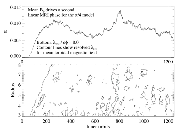
Figure 3: Contour lines of the resolved MRI from the mean toroidal field $\lambda_{crit}^{\overline{B_{\phi}}}$ with the evolution of the $\alpha$ value for the models $\pi/4$ (top) and $\pi/2$ (bottom). The contour lines show $\lambda_{crit}^{\overline{B_{\phi}}}=8$. The strong mean toroidal field amplifies the turbulence.

Figure 4: Contour lines of the resolved MRI from the mean toroidal field $\lambda_{crit}^{\overline{B_{\phi}}}$ with the evolution of the $\alpha$ value for the models $\pi$ (top) and $2\pi$ (bottom). The contour lines show $\lambda_{crit}^{\overline{B_{\phi}}}=8$. Here, the mean toroidal field is weaker and not resolved by the code.

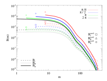
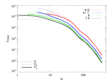
Figure 5: Left: Magnetic field distribution in Fourier space over azimuthal wave number for all models and magnetic field components. Right: Same for the velocity field. Values are from the midplane and time averaged between 800 and 1200 inner orbits.

$\Delta\phi$	$\rm\alpha_{SS}^{total}10^{-3}$	$\rm\frac{\alpha_{SS}^{mean}}{\alpha_{SS}^{total}}$	$\rm\alpha_{SS}^{turb}10^{-3}$	$\rm\alpha^{SH}_{\phi\phi}10^{-3}$	$\rm\alpha^{NH}_{\phi\phi}10^{-3}$	Parity	$\rm V_{RMS}$ $[c_{s}]$
$\pi/4$	$11.8\pm 2.3$	0.33	$8.9\pm 1.6$	$-3.4\pm 0.9$	$3.3\pm 0.8$	$-0.2\pm 0.4$	$0.125\pm 0.009$
$\pi/2$	$9.3\pm 0.9$	0.19	$7.8\pm 0.7$	$-2.8\pm 0.6$	$3.1\pm 0.7$	$-0.2\pm 0.5$	$0.148\pm 0.006$
$\pi$	$5.6\pm 0.5$	0.12	$5.0\pm 0.4$	$-2.4\pm 0.3$	$2.1\pm 0.3$	$-0.1\pm 0.5$	$0.112\pm 0.005$
$2\pi$	$5.4\pm 0.4$	0.08	$5.0\pm 0.3$	$-2.3\pm 0.2$	$2.1\pm 0.2$	$0.2\pm 0.4$	$0.113\pm 0.005$

Table 1: Model overview. From left to right: Azimuthal domain; Volume integrated total stress; Relation between $\rm\alpha_{SS}^{mean}$ to $\rm\alpha_{SS}^{turb}$; $\rm\alpha_{SS}^{turb}$ stress; Value of dynamo $\rm\alpha^{SH}_{\phi\phi}$ for southern hemisphere (lower disk); Value of dynamo $\rm\alpha^{NH}_{\phi\phi}$ for northern hemisphere (upper disk).

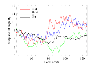
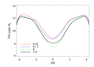
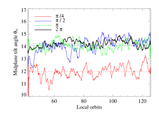
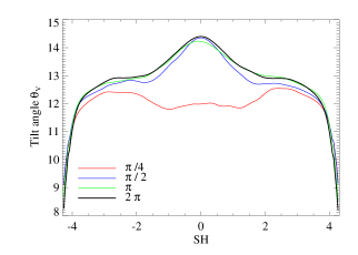
Figure 6: Top left: Midplane magnetic tilt angle over time for all models. Bottom left: Time averaged magnetic tilt angle for all models. Top right: Midplane velocity tilt angle over time for all models. Bottom right: Time averaged velocity tilt angle for all models.

Two-point correlation function

The two-point correlation function, specified for MRI by Guan et al. (2009), allows to study the locality and anisotropy of the turbulence. We measure the tilt angle for the magnetic $\sin{2\theta_{B}}=|B_{r}B_{\phi}|/B^{2}$ and the turbulent velocity field $\sin{2\theta_{V}}=|V^{\prime}_{r}V^{\prime}_{\phi}|/V^{\prime 2}$ at 4.5 AU. In Fig. 6, we plot the time evolution, top, and the vertical distribution, bottom, of the magnetic tilt angle $\theta_{B}$, left, and the velocity $\theta_{V}$, right. The time evolution of the magnetic tilt angle $\theta_{B}$ is plotted in Fig. 6 top left. The $\pi/4$ and $\pi/2$ model show higher tilt angles ($\theta_{B}\sim 9^{\circ}$) with much higher time deviations as the $\pi$ and $2\pi$ model ($\theta_{B}\sim 8^{\circ}$). The $\pi/4$ model shows sudden increase of the tilt angle at 80 local orbits. At this time, the turbulence gets amplified due to strong axisymmetric fields, see Fig. 3. The time averaged vertical profile of $\theta_{B}$ is plotted in Fig. 6, bottom left. The tilt angle present the highest values in the coronal region. Here, we see again higher $\theta_{B}$ values for the $\pi/4$ and $\pi/2$. The $\pi$ model shows smaller $\theta_{B}$ at the midplane compared to $2\pi$ which is an artefact of the selected time average. Both models present equal values after 100 local orbits, see Fig. 6, top left.

We do the same analysis for the velocity tilt angle $\theta_{V}$. The time evolution for $\theta_{V}$ does not show strong fluctuations. At the midplane, we measure a time averaged velocity tilt angle of $\theta_{V}\sim 14^{\circ}$ for all models except of $\pi/4$. The $\pi/4$ model shows a systematic lower tilt angle $\theta_{V}^{\pi/4}\sim 12^{\circ}$. This becomes also visible in the vertical profile. Here all models, except $\pi/4$, show a peak of $\theta_{V}$ at the midplane. The reason is unresolved density waves. The $\pi/4$ model does not resolve the density waves with $\rm m=4$. At $\rm m=4$, all models show the highest turbulent amplitude in the radial velocity. For model $\pi/2$ it matches the size of the domain and it is not captured by model $\pi/4$. The fast drop of magnetic and velocity tilt angles above 4 scale height could be due to boundary effects.

We calculate the two-point correlation functions in the $r-\phi$ plane: $\epsilon_{V}=<\delta V_{i}(\vec{x})\delta V_{i}(\vec{x}+\Delta\vec{x})>$ and $\epsilon_{B}=<\delta B_{i}(\vec{x})\delta B_{i}(\vec{x}+\Delta\vec{x})>$ with $\vec{x}={r,\phi}$. In Fig. 7 and Fig. 8 we present the two-point correlation function at 5 AU at 1 scale height with $\Delta r=2H=0.7AU$ and the total $\phi$ domain $r\Delta\phi=\phi^{Domain}/0.07H$. For the $2\pi$ model we have around $\rm 90H$ ($2\pi/0.07$). The corresponding major and minor wavelength are calculated using the half width at half maximum (HWHM) in units of $\rm H$ $(\rm H|_{\rm 5AU}=0.35AU)$. It measures the distance between the center $\epsilon=1.0$ and $\epsilon=0.5$ along the major $\lambda_{maj}$ and minor $\lambda_{min}$ axis, see footnote 7 in Guan et al. (2009). We measure the two-point correlation function at different heights. The results between $\rm\pm 2H$ are similar and we present the values at 1 scale height. For the velocity, the $\rm\lambda_{maj}$ of the $\pi/4$ run is $1.1H$. The $\pi$ and $2\pi$ run present both a value of $1.9H$. We find a similar increase for the $\rm\lambda_{min}$, from $0.19H$ for $\pi/4$ to $0.24H$ and $0.23H$ for model $\pi$ and $2\pi$. The values of the $\pi/2$ model present the highest values, $\rm\lambda_{maj}=2.0H$ and $\rm\lambda_{min}=0.29H$. This is again due to the peak of turbulent radial velocity at domain size, see Fig. 5, right. It is visible in the magnetic fields too. The $\rm\lambda_{min}$ value for the magnetic fields are 0.14 H, except the $\pi/2$ model with 0.16 H. The $\rm\lambda_{maj}$ increases with increasing the azimuthal domain, the $\pi/4$ model with $1.1H$ to $1.4H$, $1.6H$ and $1.7H$ for the full $2\pi$. All results of the tilt angels, major and minor wavelengths are summarised in Table 2.

$\Delta\phi$	$\rm\theta_{V}$	$\rm\lambda_{maj}^{Vel.}$	$\rm\lambda_{min}^{Vel.}$	$\rm\theta_{B}$	$\rm\lambda_{maj}^{Mag.}$	$\rm\lambda_{min}^{Mag.}$
$\pi/4$	12.0	1.1 H	0.19 H	9.1	1.1 H	0.14 H
$\pi/2$	14.1	2.0 H	0.29 H	8.9	1.4 H	0.16 H
$\pi$	14.1	1.9 H	0.24 H	7.7	1.6 H	0.14 H
$2\pi$	14.2	1.9 H	0.23 H	8.2	1.7 H	0.14 H

Table 2: Two-point correlation values for all runs. From left to right: Azimuthal domain, correlation angle for the velocity, wavelength of the major axis, wavelength of the minor axis, correlation angle for the magnetic field, wavelength of the major axis, wavelength of the minor axis.

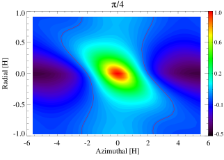
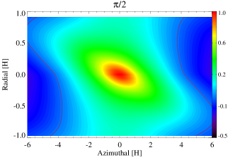
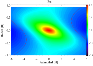
Figure 7: Contour plot of the two-point velocity correlation function at 1 scale height at 5 AU. The red line shows zero contour.

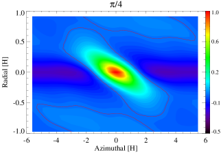
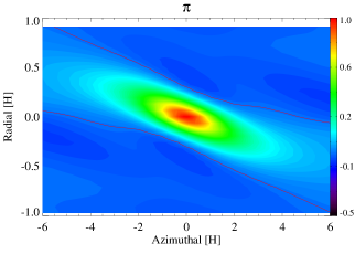
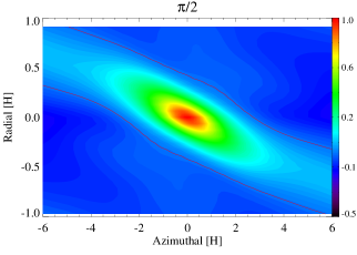
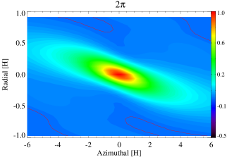
Figure 8: Contour plot of the two-point magnetic field correlation function at 1 scale height at 5 AU. The red line shows zero contour.

The models with $\pi/4$ and $\pi/2$ show an amplified turbulence. The $\phi^{extent}$ affects the large scale and small scale turbulent properties. Only an azimuthal domain of $\pi$ does reproduce similar large scale and small scale turbulent properties as in the full $2\pi$ run. The strong mean field generated by the $\alpha\Omega$ dynamo are responsible for the MRI amplification.

3.2 Mean field evolution

A typical feature of MRI in stratified disks is an oscillating toroidal magnetic field, generated by oscillating radial magnetic field. This feature is well known as ’butterfly’ pattern, which wings appear due to the buoyant movement of the toroidal field from the midplane to upper layers. The timescale of these oscillation is around ten local orbits. Recent work in local box simulations showed the context between this oscillating magnetic field and a dynamo process (Gressel, 2010; Simon et al., 2011; Hawley et al., 2011; Guan & Gammie, 2011). In this section we investigate the evolution of this axisymmetric magnetic fields and the connection to the dynamo process.

The parity and butterfly pattern

In Fig. 9, top, we present the time evolution of axisymmetric radial and toroidal magnetic field over height. The values are normalised over the initial toroidal field. The generated toroidal magnetic field, Fig. 9 (second from top) is around one order of magnitude higher than the radial magnetic field. We observe a change of sign every 5 local orbits. The butterfly wings are mostly antisymmetric with respect to the midplane. To quantify the symmetry we determine the parity of the mean magnetic field. We calculate the symmetric (S) and asymmetric (AS) magnetic field component: $B^{\rm S}_{r,\theta,\phi}=0.5(B_{{r,\theta,\phi}}^{\rm NH}+B_{{r,\theta,\phi}}^{\rm SH})$ and $B^{\rm AS}_{r,\theta,\phi}=0.5(B_{{r,\theta,\phi}}^{\rm NH}-B_{{r,\theta,\phi}}^{\rm SH})$ with the values of the northern (NH) and southern (SH) hemisphere (SH). The parity

$$Parity=\frac{E^{D}-E^{Q}}{E^{D}+E^{Q}}$$

is determined with total dipole and quadrupole energy components $\rm E^{D}=(B^{AS}_{r})^{2}+(B^{S}_{\theta})^{2}+(B^{AS}_{\phi})^{2}$ and $\rm E^{Q}=(B^{S}_{r})^{2}+(B^{AS}_{\theta})^{2}+(B^{S}_{\phi})^{2}$. The toroidal field is much larger then the radial and theta magnetic field. It is possible to define a symmetric (Quadrupole) or antisymmetric (Dipole) configuration as the total parity is set by the toroidal field. Then, a parity of -1 defines a pure symmetric configuration (Quadrupole) while a parity of +1 defines a pure antisymmetric configuration (Dipole). The time evolution of the total parity is plotted in Fig. 10, top, for all models. The total parity starts with -1 as the initial field $B_{\phi}$ is symmetric. The parity of only $B_{r}$ and $B_{\theta}$ is plotted in Fig. 10, bottom, and present a similar time evolution. Both parities change sign several times during the simulation for all models. The time averaged values (400 - 1200 inner orbits) show strong deviations around zero parity, see Table 1. Only the $2\pi$ model is mostly antisymmetric for the simulation time. The contour plot of total parity over height, Fig. 9 third plot from top, shows the correlation between the parity and the ’butterfly’ pattern. The symmetry of the mean toroidal field in respect to the midplane sets the total parity. Even the total parity is mostly antisymmetric (yellow, +1) there is a change of the parity to symmetric for two butterfly cycles between 80 and 100 local orbits (also visible in Fig. 10, solid line).

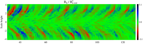
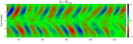
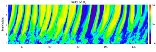
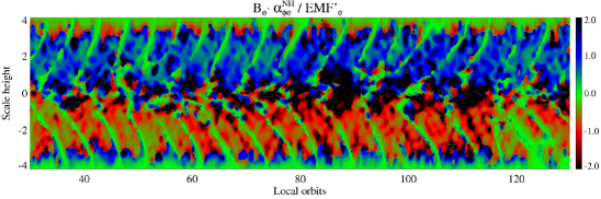
Figure 9: Top to bottom: 1. Mean radial magnetic field over height and time. 2. Mean toroidal magnetic field over height and time. 3. Contour plot of the parity over height and time. 4. Contour plot of $\overline{B_{\phi}}\alpha_{\phi\phi}^{NH}/EMF^{\prime}_{\phi}$ over height and time. All plots are made for model $2\pi$ at 4.5 AU.

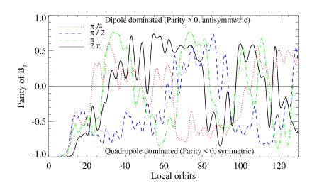
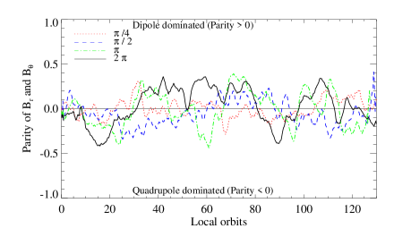
Figure 10: Parity of mean toroidal magnetic field (top) and of mean poloidal field (bottom).

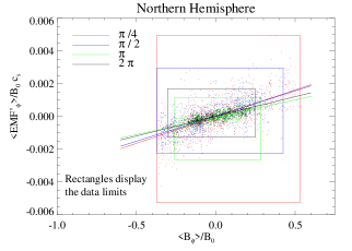
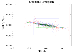
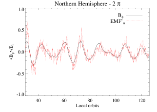
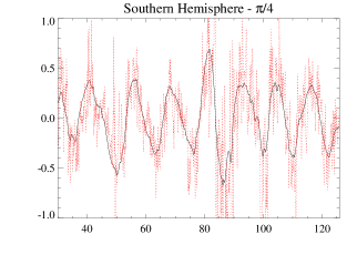
Figure 11: Top left: Correlation between the mean toroidal magnetic field and the turbulent EMF component $EMF^{\prime}_{\phi}$ for the northern (upper) hemisphere of the disk and for all models. Rectangles show the limits of the data values. Bottom left: Correlation between the mean toroidal magnetic field and the turbulent EMF component $EMF^{\prime}_{\phi}$ for the southern hemisphere of the disk and for all models. Top right: Time evolution of mean toroidal field (solid line), over-plotted with the turbulent EMF (red dotted line) divided by $\alpha_{\phi\phi}^{NH}$ for model $2\pi$. Bottom right: Time evolution of mean toroidal field (solid line), over-plotted with the turbulent $EMF^{\prime}_{\phi}$ (red dotted line) divided by $\alpha_{\phi\phi}^{SH}$ for model $\pi/4$.

$\alpha\Omega$ Dynamo

In mean field theory, there is a mechanism to generate large-scale magnetic fields by a turbulent field. In case of an $\alpha\Omega$ dynamo (Krause & Raedler, 1980) there should be a correlation between the turbulent toroidal electromotive force ($EMF^{\prime}_{\phi}$) component and the mean toroidal magnetic field,

$$\rm\overline{EMF^{\prime}_{\phi}}=\alpha_{\phi\phi}\overline{B_{\phi}}\rm+\ higher\ derivatives\ of\ \overline{B}$$

with $EMF^{\prime}_{\phi}=v^{\prime}_{r}B^{\prime}_{\theta}-v^{\prime}_{\theta}B^{\prime}_{r}$. The sign of $\rm\alpha_{\phi\phi}$ has to change for the southern and northern hemisphere. The correlation is plotted in Fig. 11, left, for the northern hemisphere (top) and the southern hemisphere (bottom). We get a positive sign for the $\rm\alpha_{\phi\phi}$ in the northern hemisphere ($\rm\alpha_{\phi\phi}^{NH}$) of the disk (Fig. 11 top) and a negative sign in the southern hemisphere ($\rm\alpha_{\phi\phi}^{SH}$). This result was predicted for stratified accretion disks (Ruediger & Kichatinov, 1993) and also indicated in global simulations (Arlt & Rüdiger, 2001). Each dot in Fig. 11 left, represent a result from a single time snapshot. The boxes show the limits of the values for each model. The $\pi/4$ and $\pi/2$ model show higher amplitudes in the mean field $\overline{B_{\phi}}$ as well as in the $EMF^{\prime}_{\phi}$ fluctuations. All values of $\rm\alpha_{\phi\phi}$ are determined using a robust regression method and summarized in Table 1. A time evolution of the mean field and the turbulent $EMF^{\prime}_{\phi}$ is presented in Fig. 11, right, for model $2\pi$, top, and model $\pi/4$, bottom. In Fig. 11 right, we divide the turbulent $\rm EMF^{\prime}_{\phi}$ with the measured $\rm\alpha_{\phi\phi}$ (see also Table 1). The $\pi/4$ run shows higher fluctuations compared to the $2\pi$ run. A time evolution of $\rm B_{\phi}\cdot\alpha_{\phi\phi}^{NH}/EMF^{\prime}_{\phi}$ over height is presented in Fig. 9, bottom. We see that the sign of $\rm\alpha_{\phi\phi}$ is well defined for the two hemispheres, reaching up to 3 scale heights of the disk.

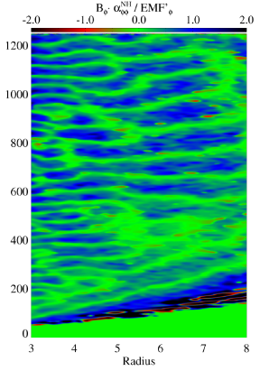
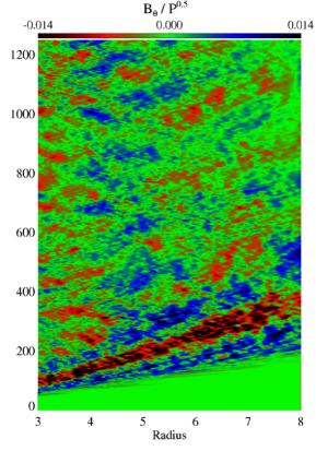
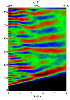
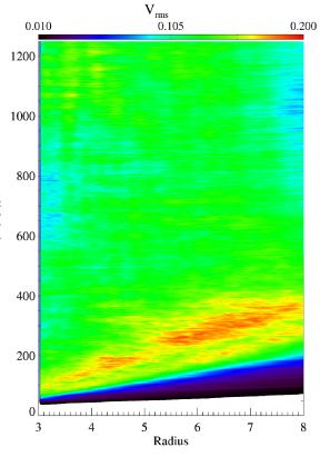
Figure 12: Top left: Contour plot of $\overline{B_{\phi}}\cdot\alpha_{\phi\phi}^{NH}/EMF^{\prime}_{\phi}$ over radius and time (see also Fig 9, bottom). Top right: Mean toroidal magnetic field over radius and time. Bottom left: Mean $\theta$ magnetic field over radius and time. Bottom right: Turbulent RMS velocity over radius and time. All plots are made for model $2\pi$ in the northern hemisphere.

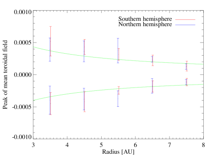
Figure 13: Radial distribution of the peaks of mean toroidal magnetic field. Values from the northern hemisphere are in red and from the southern hemisphere in blue, (see also Fig. 12, top right).

3.3 Mean fields over radius

In this section we study the development of the mean magnetic fields along radius. We show results from our full $2\pi$ model as it represents the most realistic physical domain size. A contour plot of mean toroidal field, normalised over the square root of the pressure, is presented in Fig. 12, top right, over radius and time. All results in Fig. 12 are averaged along azimuth and along $\theta$ between the midplane and two disk scale heights in the northern hemisphere. Fig. 12, top right, shows the irregular change of sign for the mean toroidal magnetic field along radius. The timescale of the ”butterfly” oscillations at a given radius can change because of radial interactions. The timescale of reversals of the toroidal magnetic field does vary from the ten local orbital line (see Fig. 12, top right, horizontal homogeneous $B_{\phi}$). The mean field configuration along radius can strongly affect the accretion stress, see Fig. 3. The distribution of mean $B_{\theta}$ over radius is more irregular compared to the toroidal field, see Fig. 12 bottom left, although we observe a preferred sign of mean $B_{\theta}$ for a specific radial location, e.g. positive over time between 4 and 5 AU. A time evolution over radius of $\rm B_{\phi}\cdot\alpha_{\phi\phi}^{NH}/EMF^{\prime}_{\phi}$ , Fig. 12 top left, shows again the positive sign of $\rm\alpha_{\phi\phi}$ in the northern hemisphere (see also Fig. 9, bottom). By definition, the $\rm\alpha_{\phi\phi}$ presents the same distribution along radius as the mean toroidal magnetic field. In contrast we do not find a correlation between the turbulent velocity of the gas and the distribution of mean magnetic fields. Fig. 12, bottom right, presents $\rm v_{rms}$ over radius and time for the northern hemisphere. The RMS velocity is about $0.1c_{s}$, nearly constant over radius and time. A time average of $\rm v_{rms}$ is given in Table 1 for all models. We again emphasize the lower turbulent velocity in the $\pi/4$, compared to $\pi/2$, due to the lack of the radial velocity peak (see Fig. 5, right).

In our previous work we have shown the $1/r$ profile for the turbulent magnetic fields (Flock et al., 2011). Because of the time oscillations, it is difficult to estimate a radial profile for the mean magnetic field. To determine a time averaged radial profile of the mean toroidal field we measure the amplitude values of the oscillations. We use five different radial locations to measure the peak values of the mean toroidal field. The results are plotted in Fig. 13 for the southern (blue) and northern hemisphere (red). The amplitudes of mean toroidal field decreases with radius. The relative low number of values and their high standard deviation makes it difficult to fit. A $1/r$ profile would apply (Fig. 13, green solid line). The values in both hemispheres look quite symmetric (Fig. 9, blue and red) and we do not see a preferred hemisphere for the mean field generation.

4 Discussion

After the saturation of MRI, the initial magnetic field configuration is lost. Each model develops oscillating mean magnetic fields which appears to be strongest in the $\pi/4$ and $\pi/2$ run. The strength of turbulence follows this trend. The mean fields are generated by a dynamo process which relies on the symmetry and on the strength of the turbulent field. We measure higher dynamo coefficient $\alpha_{\phi\phi}$ for the $\pi/2$ and $\pi/4$ model as well as higher Maxwell stresses. This agrees with the correlation between Maxwell stress and dynamo coefficient, found by Rekowski et al. (2000). The effect of increased magnetic energy at domain size seems to be independent of resolution in stratified simulations (compare Fig. 12, bottom left, model FO and PO in Flock et al. (2011)) but not present in unstratified simulations (compare Fig. 9b in Sorathia et al. (2011)) as they do not develop a dynamo.

Energy pile up and magnetic dynamo

Which physical process is sensitive to the domain size and lead to the increased mean toroidal fields in $\pi/4$ and $\pi/2$ models ? The first mechanism leads to the dynamo process as it generates axisymmetric magnetic fields out of the turbulence. Another way to transport magnetic energy at domain size could be due to an inverse energy cascade. Johansen et al. (2009) showed in local box simulations that the Keplerian advection term in the induction equations drives an inverse energy cascade. This will lead to a transport of energy to larger scales. Also Rüdiger et al. (2007) found in Taylor-Couette experiments that MRI, launched from a toroidal field, will have most of magnetic energy at the $\rm m=1$ and $\rm m=0$ mode.

Another open question is the sign of $\alpha_{\phi\phi}$ in global simulations. We find a positive $\rm\alpha_{\phi\phi}$, independent of the azimuthal domain size. This positive $\rm\alpha_{\phi\phi}$ has been indicated for global simulations by Arlt & Rüdiger (2001). Local simulations show a negative $\rm\alpha_{\phi\phi}$ (Brandenburg et al., 1995; Brandenburg & Donner, 1997; Rüdiger & Pipin, 2000; Ziegler & Rüdiger, 2000; Davis et al., 2010; Gressel, 2010). The reason of stronger mean fields in reduced azimuthal models as well as the positive sign of $\rm\alpha_{\phi\phi}$ in global simulations has to be investigated in future work. One possibility would be to implement the ’Test field’ method and to measure other components of the dynamo and diffusivity tensor, as it was done in Gressel (2010).

4.1 Time variability of accretion stress.

Oscillating mean field are organized in elongated radial patches, normally following the time-line of ten local orbits. It can occur that for a given time, mean toroidal field of one sign covers the whole radial extent (3 - 8 AU). In such a case, temporal linear MRI will lead to a peak in accretion stress, Fig. 3. The effect of mean toroidal field, stretching over the whole radius, is independent on the azimuthal domain size, compare Fig. 12 top right. The amplification of accretion stress due to linear MRI, is visible only in the $\pi/4$ model, as it present strongest amplitudes in the mean toroidal magnetic field.

Correlation functions

We confirm the results of recent stratified global simulations by Beckwith et al. (2011). We find similar correlation angles (around $9^{\circ}$) and wavelengths (around H) for the magnetic field. A larger correlation length is expected because of the relative low resolution per scale height compared to local simulations (Guan et al., 2009; Hawley et al., 2011; Sorathia et al., 2011). Recent unstratified global simulations Sorathia et al. (2011) suggest a magnetic tilt angle of around $13^{\circ}$ for converged MRI turbulence. It remains still unclear how this could be applied for stratified disks with a minimum of $\theta_{B}$ at the midplane. We found a magnetic tilt angle of around $13^{\circ}$ above 2 scale heights. As discussed in Flock et al. (2011) we believe to find convergence with resolutions around 32/64 grid cells per pressure scale height. Here, a Fargo MHD approach as used in Sorathia et al. (2011) would be helpful.

5 Summary

We have studied the impact of different azimuthal extents in 3D global stratified MHD simulations of accretion disks onto the saturation level of MRI with an initial toroidal magnetic field.

• Turbulence in restricted domain sizes like $\pi/2$ and $\pi/4$ is amplified due to strong toroidal mean field oscillations. For these runs, the $\lambda_{crit}$ of the mean field is resolved leading to a temporal magnification of the $\alpha_{SS}$ value and increased total magnetic energy. In addition, radial superpositions of such strong mean fields can drive to a strong episodic increase of accretion. The time averaged total $\alpha_{SS}$ is $1.2\pm 0.2\cdot 10^{-2}$ for model $\pi/4$, $9.3\pm 0.9\cdot 10^{-3}$ for model $\pi/2$ and converge to $5.5\pm 0.5\cdot 10^{-3}$ for both models $\pi$ and $2\pi$.

• We find a positive dynamo $\alpha_{\phi\phi}$ for all models, a positive correlation between the turbulent $EMF^{\prime}_{\phi}$ and the mean toroidal magnetic field in the upper (northern) hemisphere. For the $2\pi$ model we found $\rm\alpha_{\phi\phi}^{North}=2.1\pm 0.2\cdot 10^{-3}$. The $\pi/2$ and $\pi/4$ present higher $\rm\alpha_{\phi\phi}$ values but with stronger fluctuations in $EMF^{\prime}_{\phi}$ and mean $B_{\phi}$.

• The $\pi/4$ and $\pi/2$ models show higher tilt angles and smaller correlation wavelengths in the two-point correlation of velocity and magnetic field compared to the $\pi$ and $2\pi$ models. We find $\rm\theta_{t}^{vel}=14^{\circ}$ for models $\geq\pi/2$ and $\rm\theta_{t}^{vel}=12^{\circ}$ for model $\pi/4$. The $\pi/4$ model does not resolve the peak radial velocity at $\rm m=4$. The tilt angles for the magnetic fields are smaller. At the midplane we observe time averaged magnetic tilt angles between $\rm\theta_{B}=8-9^{\circ}$ increasing up to $\rm\theta_{B}=12-13^{\circ}$ in the corona. For the full $2\pi$ model we found $\rm\lambda_{maj}^{vel}=1.9H$ and $\rm\lambda_{maj}^{mag}=1.7H$.

• The parity of the mean magnetic fields is a mixture of dipole and quadrupole for all models. The total parity is set by the oscillating toroidal field. The timescale of symmetry change between dipole and quadrupole is around 40 local orbits. The time evolution of the parity is distinct in each model. The $2\pi$ model remains longer in a dipole (antisymmetric) dominated configuration for the simulation time.

We conclude: In global MRI simulations of accretion disks an azimuthal domain of at least $\pi$ $(180^{\circ})$ is needed to present the most realistic turbulent and mean field evolution as the full $2\pi$ model. Here, the $\alpha\Omega$ dynamo plays a key role in determining the saturation level of MRI. Restricted domains of $\pi/4$ and $\pi/2$ amplify the MRI turbulence due to a stronger axisymmetric magnetic fields.

We thank Andrea Mignone for providing us with the newest code version and the discussion on the numerical configuration. We thank Sebastien Fromang for the helpful comments on the global models. We thank also Günther Rüdiger and Rainer Arlt for their comments on the manuscript. We thank Geoffroy Lesur for the discussion about the dynamo effect. H. Klahr, N. Dzyurkevich and M. Flock have been supported in part by the Deutsche Forschungsgemeinschaft DFG through grant DFG Forschergruppe 759 ”The Formation of Planets. The Critical First Growth Phase”. Neal Turner was supported by a NASA Solar Systems Origins grant through the Jet Propulsion Laboratory, California Institute of Technology, and by an Alexander von Humboldt Foundation Fellowship for Experienced Researchers. Parallel computations have been performed on the Theo cluster of the MaxPlanck Institute for Astronomy Heidelberg as well as the GENIUS Blue Gene/P cluster both located at the computing center of the MaxPlanck Society in Garching.

References

- Arlt & Brandenburg (2001) Arlt, R. & Brandenburg, A. 2001, A&A, 380, 359
- Arlt & Rüdiger (2001) Arlt, R. & Rüdiger, G. 2001, A&A, 374, 1035
- Armitage (1998) Armitage, P. J. 1998, ApJ, 501, L189
- Balbus & Hawley (1991) Balbus, S. A. & Hawley, J. F. 1991, ApJ, 376, 214
- Balbus & Hawley (1998) —. 1998, Reviews of Modern Physics, 70, 1
- Beckwith et al. (2011) Beckwith, K., Armitage, P. J., & Simon, J. B. 2011, ArXiv e-prints
- Blackman (2010) Blackman, E. G. 2010, Astronomische Nachrichten, 331, 101
- Brandenburg & Donner (1997) Brandenburg, A. & Donner, K. J. 1997, MNRAS, 288, L29
- Brandenburg et al. (1995) Brandenburg, A., Nordlund, A., Stein, R. F., & Torkelsson, U. 1995, ApJ, 446, 741
- Brandenburg & Subramanian (2005) Brandenburg, A. & Subramanian, K. 2005, Phys. Rep., 417, 1
- Brandenburg & von Rekowski (2007) Brandenburg, A. & von Rekowski, B. 2007, Memorie della Societa Astronomica Italiana, 78, 374
- Davis et al. (2010) Davis, S. W., Stone, J. M., & Pessah, M. E. 2010, ApJ, 713, 52
- Dzyurkevich et al. (2010) Dzyurkevich, N., Flock, M., Turner, N. J., Klahr, H., & Henning, T. 2010, A&A, 515, A70
- Elstner et al. (1996) Elstner, D., Ruediger, G., & Schultz, M. 1996, A&A, 306, 740
- Fleming & Stone (2003) Fleming, T. & Stone, J. M. 2003, ApJ, 585, 908
- Flock et al. (2010) Flock, M., Dzyurkevich, N., Klahr, H., & Mignone, A. 2010, A&A, 516, A26
- Flock et al. (2011) Flock, M., Dzyurkevich, N., Klahr, H., Turner, N. J., & Henning, T. 2011, ArXiv e-prints
- Foglizzo & Tagger (1995) Foglizzo, T. & Tagger, M. 1995, A&A, 301, 293
- Fromang (2010) Fromang, S. 2010, A&A, 514, L5
- Fromang & Nelson (2006) Fromang, S. & Nelson, R. P. 2006, A&A, 457, 343
- Fromang & Nelson (2009) —. 2009, A&A, 496, 597
- Gardiner & Stone (2005) Gardiner, T. A. & Stone, J. M. 2005, Journal of Computational Physics, 205, 509
- Gellert et al. (2007) Gellert, M., Rüdiger, G., & Fournier, A. 2007, Astronomische Nachrichten, 328, 1162
- Gressel (2010) Gressel, O. 2010, MNRAS, 404
- Guan & Gammie (2011) Guan, X. & Gammie, C. F. 2011, ApJ, 728, 130
- Guan et al. (2009) Guan, X., Gammie, C. F., Simon, J. B., & Johnson, B. M. 2009, ApJ, 694, 1010
- Hawley (2000) Hawley, J. F. 2000, ApJ, 528, 462
- Hawley & Balbus (1991) Hawley, J. F. & Balbus, S. A. 1991, ApJ, 376, 223
- Hawley & Balbus (1992) —. 1992, ApJ, 400, 595
- Hawley et al. (1995) Hawley, J. F., Gammie, C. F., & Balbus, S. A. 1995, ApJ, 440, 742
- Hawley et al. (1996) —. 1996, ApJ, 464, 690
- Hawley et al. (2011) Hawley, J. F., Guan, X., & Krolik, J. H. 2011, ArXiv e-prints
- Heinemann & Papaloizou (2009) Heinemann, T. & Papaloizou, J. C. B. 2009, MNRAS, 397, 64
- Inutsuka & Sano (2005) Inutsuka, S. & Sano, T. 2005, ApJ, 628, L155
- Johansen et al. (2009) Johansen, A., Youdin, A., & Klahr, H. 2009, ApJ, 697, 1269
- Krause & Raedler (1980) Krause, F. & Raedler, K.-H. 1980, Mean-field magnetohydrodynamics and dynamo theory, ed. Williams, L. O.
- Lesur & Ogilvie (2008a) Lesur, G. & Ogilvie, G. I. 2008a, MNRAS, 391, 1437
- Lesur & Ogilvie (2008b) —. 2008b, A&A, 488, 451
- Matsumoto & Tajima (1995) Matsumoto, R. & Tajima, T. 1995, ApJ, 445, 767
- Miller & Stone (2000) Miller, K. A. & Stone, J. M. 2000, ApJ, 534, 398
- Miyoshi & Kusano (2005) Miyoshi, T. & Kusano, K. 2005, Journal of Computational Physics, 208, 315
- Noble et al. (2010) Noble, S. C., Krolik, J. H., & Hawley, J. F. 2010, ApJ, 711, 959
- Papaloizou & Terquem (1997) Papaloizou, J. C. B. & Terquem, C. 1997, MNRAS, 287, 771
- Rekowski et al. (2000) Rekowski, M. v., Rüdiger, G., & Elstner, D. 2000, A&A, 353, 813
- Rüdiger et al. (2007) Rüdiger, G., Hollerbach, R., Gellert, M., & Schultz, M. 2007, Astronomische Nachrichten, 328, 1158
- Rüdiger & Pipin (2000) Rüdiger, G. & Pipin, V. V. 2000, A&A, 362, 756
- Ruediger & Kichatinov (1993) Ruediger, G. & Kichatinov, L. L. 1993, A&A, 269, 581
- Sano et al. (2000) Sano, T., Miyama, S. M., Umebayashi, T., & Nakano, T. 2000, ApJ, 543, 486
- Simon et al. (2011) Simon, J. B., Hawley, J. F., & Beckwith, K. 2011, ApJ, 730, 94
- Sorathia et al. (2010) Sorathia, K. A., Reynolds, C. S., & Armitage, P. J. 2010, ApJ, 712, 1241
- Sorathia et al. (2011) Sorathia, K. A., Reynolds, C. S., Stone, J. M., & Beckwith, K. 2011, ArXiv e-prints
- Stone et al. (1996) Stone, J. M., Hawley, J. F., Gammie, C. F., & Balbus, S. A. 1996, ApJ, 463, 656
- Terquem & Papaloizou (1996) Terquem, C. & Papaloizou, J. C. B. 1996, MNRAS, 279, 767
- Turner et al. (2010) Turner, N. J., Carballido, A., & Sano, T. 2010, ApJ, 708, 188
- Umebayashi (1983) Umebayashi, T. 1983, Progress of Theoretical Physics, 69, 480
- Umebayashi & Nakano (2009) Umebayashi, T. & Nakano, T. 2009, ApJ, 690, 69
- Uribe et al. (2011) Uribe, A., Klahr, H., Flock, M., & Henning, T. 2011, ArXiv e-prints
- Wardle (2007) Wardle, M. 2007, Ap&SS, 311, 35
- Ziegler & Rüdiger (2000) Ziegler, U. & Rüdiger, G. 2000, A&A, 356, 1141