Photometry and Photometric Redshift catalogs for the Lockman Hole Deep Field

Abstract

We present broad band photometry and photometric redshifts for 187611 sources located in $\sim 0.5\,\rm{deg}^{2}$ in the Lockman Hole area. The catalog includes 389 X-ray detected sources identified with the very deep XMM-Newton observations available for an area of $0.2\,\rm{deg}^{2}$. The source detection was performed on the $R_{c}$, $z^{\prime}$ and $B$ band images and the available photometry is spanning from the far ultraviolet to the mid infrared, reaching in the best case scenario 21 bands. Astrometry corrections and photometric cross-calibrations over the entire dataset allowed the computation of accurate photometric redshifts. Special treatment is undertaken for the X-ray sources, the majority of which is active galactic nuclei. Comparing the photometric redshifts to the available spectroscopic redshifts we achieve for normal galaxies an accuracy of $\sigma_{\Delta z/(1+z)}=0.036$, with $12.7\%$ outliers, while for the X-ray detected sources the accuracy is $\sigma_{\Delta z/(1+z)}=0.069$, with $18.3\%$ outliers, where the outliers are defined as sources with ${|z_{phot}-z_{spec}|}>0.15\cdot{(1+z_{spec})}$. These results are a significant improvement over the previously available photometric redshifts for normal galaxies in the Lockman Hole, while it is the first time that photometric redshifts are computed and made public for AGN for this field.

1 Introduction

Multiwavelength surveys provide the most successful observational strategy towards the understanding of galaxies. The multiwavelength coverage provides the opportunity to compute photometric redshifts and to study the Spectral Energy Distributions (SED) for a large number of galaxies. At the same time, careful estimation of the distances of the galaxies enables the study of the intrinsic properties of the sources such as luminosities and the determination of the evolution with redshift of other fundamental parameters such as stellar masses, star formation rates, etc. Furthermore, distance measurements enable the use of galaxies as cosmological probes, for example through their clustering properties.

The distance measurement for galaxies is based on the determination of the redshift of the source, which is specified very accurately through spectroscopy. However, for large samples of sources either in deep pencil beam fields, or shallower but more extended fields, the most efficient way to compute the distance is via photometric redshifts (e.g. Budavári et al., 2000), although their accuracy is strongly depending on i) the number and the type of filters (broad-band versus intermediate-band), ii) the redshift range and type of galaxies of interest (passive, versus starforming or active galactic nuclei (AGN)).

For fields where extensive photometric datasets are available the photometric redshift technique has been employed with reliable results. For example in CFHTLS (Ilbert et al., 2006), in AEGIS (Barro et al., 2011), in COSMOS (Ilbert et al., 2009; Salvato et al., 2009), in FDF (Bender et al., 2001), in the CDFN (Barger et al., 2003) and in the CDFS (Wolf et al., 2004; Luo et al., 2010; Cardamone et al., 2010) the photometric redshifts reached an accuracy $\Delta(z_{\rm phot}-z_{\rm spec})/(1+z_{\rm spec})<0.03$, thus allowing (among other applications) a 3D mapping of the Dark Matter (Massey et al., 2007), studies of the evolution of luminosity functions of normal galaxies (e.g. Ilbert et al., 2006; Gabasch et al., 2004, 2006; Caputi et al., 2006) and AGN (e.g. Hasinger et al., 2005; Barger et al., 2005; Ebrero et al., 2009; Aird et al., 2010), the first determination of the high-z (z$>$3) logN-logS and space density from X-ray selected AGN (Brusa et al., 2009; Civano et al., 2011), Compton thick objects (e.g. Fiore et al., 2009; Luo et al., 2011), etc. Moreover, photometric redshifts are also used for the study of groups and clusters of galaxies (Giodini et al., 2009; Papovich et al., 2010; Geach et al., 2011) and much more.

Yet, not all deep and wide fields have photometric redshifts of comparable accuracy, thus limiting any study to the parameter space allowed by a given field. Only reliable photometric redshifts in all the fields will allow a complete exploitation of the total telescope time devoted to survey studies in the last ten years. Keeping this is mind, here we present optically based extensive photometry and photometric redshift catalogs for the Lockman Hole Deep Field.

The Lockman Hole is the area on the sky with the lowest galactic hydrogen column density along the line of sight ($N_{H}\approx 5.7\,10^{19}\rm{cm}^{-2}$, Lockman et al. 1986; Schlegel et al. 1998). This physical characteristic provides the opportunity to perform extragalactic observations without significant absorption of the radiation in the soft X-rays and the ultra-violet and with minimal galactic cirrus emission in the infrared. For this reason the field has been observed in all energy bands from the Radio to the X-rays. A detailed overview of the various observations is given in Rovilos et al. (2009).

Up to now the spectroscopic follow up was dedicated to sources detected in specific bands (X-ray, infrared, radio). In addition, the photometry of the field was lacking crucial bands such as J and K, hampering the possibility to compute accurate photometric redshifts. The only public photometric redshifts for approximately half of the area of the field examined in this work are available via the SWIRE survey (Rowan-Robinson et al., 2008), computed using photometry in 4 broad band optical filters (U’, g’, r’, i’) and 3.6$\mu m$ and 4.5$\mu m$ mid-infrared filters from Spitzer/IRAC. Furthermore, the photometric redshifts were lacking proper treatment for the AGN.

In this work, we first cross-calibrate and then combine publicly available and private photometry from the ultra-violet to the mid infrared wavelengths, creating an extensive catalog, which we further use to compute photometric redshifts. We also separate the sample according to the X-ray emission and use the proper combination of templates and priors to achieve the best photometric redshift solution for all sources. In addition to photometry and photometric redshifts we release an up-to-date list of the spectroscopic data, both public and private, available in the field.

The layout of the paper is as follows: in §2 we describe the data we used for this work. In §3 we describe the processing of the images and the procedure we followed in order to create our catalog. In §4 we describe the method we used to compute the photometric redshifts. In §5 we present the photometric redshifts and discuss our results comparing also with previous works. Finally, in §6 we present our conclusions. All magnitudes are expressed in the AB system (Oke & Gunn, 1983).

2 Data Set

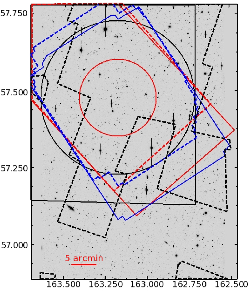
Figure 1: The area coverage of the Lockman Hole Deep Field. The image denotes the area observed in the $R_{c}$, $I_{c}$, $z^{\prime}$ filters with Subaru. The marked regions represent: U and B LBT filters (blue solid line), V, Y and z’ LBT filters (blue dashed line), $\rm{3.6\mu m}$ and $\rm{5.8\mu m}$ IRAC (red solid line), $\rm{4.5\mu m}$ and $\rm{8\mu m}$ IRAC (red dashed line), J and K UKIRT filters (black solid line). Even though the whole area is covered by SDSS, only the area enclosed in the black dashed outline has good photometry (flag=3 in the SDSS catalog). The black circle represents the area targeted by XMM-Newton and the red circle represents roughly the area targeted by the Hubble Space Telescope.

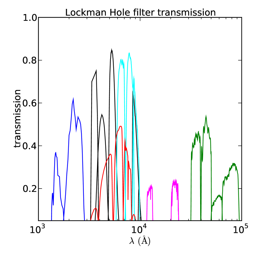
Figure 2: The filter coverage of the Lockman Hole Deep Field. Blue: GALEX (FUV, NUV), black: LBT (U, B, V, Y, z’), cyan: Subaru($\rm{R_{c}}$, $\rm{I_{c}}$, $\rm{z^{\prime}}$), red: SDSS ($\rm{u^{\prime}}$, $\rm{g^{\prime}}$, $\rm{r^{\prime}}$, $\rm{i^{\prime}}$, $\rm{z^{\prime}}$), magenta: UKIDSS (J, K), green: Spitzer ($\rm{3.6\mu m}$, $\rm{4.5\mu m}$, $\rm{5.8\mu m}$, $\rm{8.0\mu m}$).

In this section we describe the data that we used in each energy band, separated by instrument/satellite. In Fig. 1 we give an overview of the coverage of Lockman Hole area in each every band, while in Fig. 2 we present the filter transmission curves.

2.1 X-ray data

The field has been observed with XMM-Newton in the time period between April 2000 and December 2002, with a total raw exposure of 1.30 Ms for the detectors on board the satellite (EPIC MOS and EPIC pn). The field is centered at $\rm{+10^{h}52^{m}43^{s},\,+57^{\circ}28^{\prime}48^{\prime\prime}}$ and has a radius of $15^{\prime}$, thus covering an area of $\rm{\sim 0.2\,deg^{2}}$. The limiting flux in each detection band is $\rm{F_{0.5-2.0\,keV}=1.9\cdot 10^{-16}erg\,cm^{-2}s^{-1}}$ in the soft band, $\rm{F_{2.0-10.0\,keV}=9\cdot 10^{-16}erg\,cm^{-2}s^{-1}}$, in the hard band and $\rm{F_{5.0-10.0\,keV}=1.8\cdot 10^{-15}erg\,cm^{-2}s^{-1}}$, in the ultra hard band. The depth of the X-ray observations in combination with the size of the area place the field close to the Extended CDFS (ECDFS), between the very deep pencil-beam fields (e.g. CDFN and CDFS) and the more extended but shallower fields (e.g. XMM-COSMOS). In particular, the X-ray observations in the Lockman Hole Field reach one order of magnitude fainter flux limit than XMM-COSMOS in all detection bands (Table 1). The catalog of the X-ray detected sources is presented in Brunner et al. (2008) and contains a total of 409 sources with likelihood of being real detections greater than 10 (3.9$\sigma$). The catalog of optical counterparts of the X-ray sources is presented in Rovilos et al. (2011) (see also §3.2.3). In summary, the counterparts were assigned on the basis of a Likelihood Ratio (LR) technique applied to our optical and near-infrared catalogs, which reach a depth of $\rm{R_{c,lim}}$ = 26 mag and [3.6$\mu m$]_lim = 24.6 mag.

2.2 Ultra-violet data

In the far ultra-violet (FUV) and the near ultra-violet (NUV) the Lockman Hole area was observed by the Galaxy Evolution Explorer (GALEX). Here, we consider the magnitude in $\rm{3^{\prime\prime}}$ diameter aperture available in the General Release 4/5 (GR4/5). To correct the aperture photometry to total, we followed the recipe of Morrissey et al. (2007). The authors presented the growth curve analysis using as targets white dwarfs and we use the same correction factors through out the whole catalog. The Lockman Hole is part of the GALEX Deep Imaging Survey and the third quartile of the magnitude distribution reaches $\rm{FUV_{lim}=24.5\,mag}$ and $\rm{NUV_{lim}=24.5\,mag}$.

2.3 Optical data

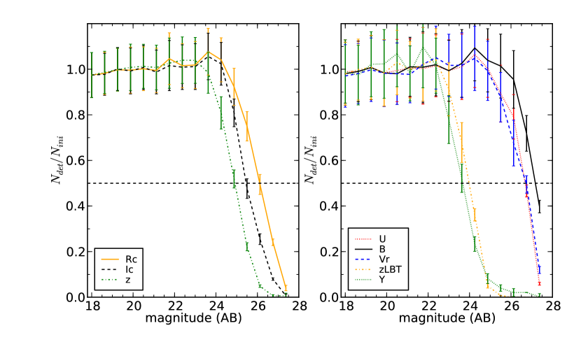
Figure 3: The completeness curves for the Subaru (left panel) and LBT (right panel) images, computed from simulated sources. The horizontal dashed line marks the 50% completeness limit.

In the optical wavelengths, our dataset consists of a compilation of observations from LBT, Subaru and SDSS. Our images exhibit very good seeing of the order of $\rm{0.9^{\prime\prime}-1^{\prime\prime}}$, such that we could retrieve almost $100\%$ of the flux for point-like sources within $\rm{3^{\prime\prime}}$ aperture (see §3.2.1 for details). Thus, we are using the $\rm{3^{\prime\prime}}$ aperture magnitudes without applying any corrections to total. In Fig. 3, we present the completeness analysis for all optical filters. We plot the ratio of detected over true number of simulated point-like sources, versus magnitude. Details on the area observed, the total exposure time, the PSF full width half maximum (FWHM), the 50% detection magnitude limit for point-like sources ($\rm{5\sigma}$, AB) and the AB to Vega correction factor for each filter, are presented in Table 2.

2.3.1 Large Binocular Telescope

We observed the Lockman Hole in the period between February 2007 and March 2009 in 5 bands ($\rm{U}$, $\rm{B}$, $\rm{V}$, $\rm{Y}$, $\rm{z^{\prime}}$) using the Large Binocular Telescope (LBT) covering an area of about $0.25\,\rm{deg^{2}}$. The reduction of the data and the number counts of the very deep observations in the U, B and V filters have been published in Rovilos et al. (2009). The two telescopes of LBT have slightly different cameras, one optimized for bluer and the other optimized for redder bands. In Rovilos et al. (2009) the published V band is the combination of two separate images ($\rm{V_{blue}}$, $\rm{V_{red}}$). However, here we are using only the $\rm{V_{red}}$ image, as the differences in the two filter curves and the low quality of the $\rm{V_{blue}}$ image, make the stacking not an option.

In addition to U, B and V photometry, in this work we also include the shallower observations in the Y and z’ filters which were reduced later in a similar manner.

2.3.2 Subaru

Complementary to our own photometry, we made use of data from the Institute for Astronomy (Hawaii) Deep Survey. Observations with the Subaru telescope between November 2001 and April 2002 provided imaging in an area of $0.53\,\rm{deg^{2}}$. The observations were carried out in the Rc, Ic and z’ filters. Details about the survey and the observations on the field can be found in Barris et al. (2004), while details on the analysis of the data can be found in §3.2.1.

2.3.3 SDSS

Unfortunately SDSS does not cover the Lockman Hole field with uniform photometric quality. However, we include SDSS (DR7, Abazajian et al. 2009) $\rm{u^{\prime}}$, $\rm{g^{\prime}}$, $\rm{r^{\prime}}$, $\rm{i^{\prime}}$, $\rm{z^{\prime}}$ photometry (fiber magnitude) when available, if $\rm{r_{AB}^{\prime}<22\,mag}$ and photometric quality flag = 3, provided in the SDSS catalog (Fig. 1 black dashed line). The first reason to use the SDSS catalog is that the observations from LBT and Subaru are very deep and the brightest sources ($\rm{R_{c}\approx 18\,mag}$) are saturated. Thus the shallower SDSS data can provide a solution to saturation problems. For example, in the $\rm{R_{c}}$ filter, 677 sources are flagged as saturated and photometry is not available. However, for 170 of these sources SDSS photometry is available and can be used to recover the SEDs and thus the photometric redshifts.

SDSS photometry is especially important for X-ray detected sources, for which we want to trace optical variability. This intrinsic property of AGN dominated systems, can affect the computation of photometric redshifts, when the photometry is obtained non-simultaneously and through multi-epoch observations. As we explain further in §3.2.3, we use the $\rm{z^{\prime}}$ band to detect the variability of a source, since in this filter we have observations from three telescopes at different epochs.

2.4 Near and Mid infrared data

2.4.1 UKIDSS data

The near-infrared view of our sources is provided by the data release 7 of the UKIRT Infrared Deep Sky Survey. The UKIDSS project is defined in Lawrence et al. (2007). UKIDSS uses the UKIRT Wide Field Camera (WFCAM; Casali et al. 2007). The photometric system is described in Hewett et al. (2006) and the photometric calibration is explained in Hodgkin et al. (2009). The Lockman Hole is part of the Deep Extragalactic Survey to be observed in the J, H and K bands. Up to now, only the J and K bands are available with limiting magnitudes of $J_{lim}=23.4$ mag and $K_{lim}=22.9$ mag (5$\rm{\sigma}$, point source) respectively. We use the $\rm{2.8^{\prime\prime}}$ aperture magnitude provided in the catalog which is already corrected to total for point-like sources. The aperture corrections were determined from the growth curve analysis of bright stars as described in Hodgkin et al. (2009).

2.4.2 Spitzer data

For the near to mid infrared wavelengths we are using observations at $\rm{3.6\mu m}$, $\rm{4.5\mu m}$, $\rm{5.8\mu m}$, $\rm{8.0\mu m}$ from the Infrared Array Camera (IRAC). Although the IRAC images are the same as the images used in Pérez-González et al. (2008), we created our own catalog. As explained in Rovilos et al. (2011) we extracted the IRAC photometry using SExtractor in dual mode using the $\rm{3.6\mu m}$ image to detect the sources in all other IRAC filters. Following Surace et al. (2005), we used the $\rm{2.8^{\prime\prime}}$ diameter aperture magnitude and applied the same corrections calculated for point-like sources. The aperture corrections have been determined performing growth curve analysis of a composite PSF consisting of 10-20 stars.

The 50% efficiency limiting magnitude of the IRAC observations is $24.6$ mag for the $\rm{3.6\mu m}$ band (2$\sigma$). We verified our photometry against the publicly available SWIRE catalog in the Lockman Hole, which is shallower and complementary to our observations. Using approximately 2400 sources in the overlapping $\rm{0.25deg^{2}}$ we find that the orthogonal distance regression gives slope of $0.995\pm 0.002$, intercept $0.19\pm 0.05$ and correlation length $0.73$, in agreement with what is found by Pérez-González et al. (2008). The offset between our photometry and the SWIRE photometry is explainable in view of the different, continuously improved pipeline used by the IRAC team in reducing the data.

3 Catalog Assembly

The photometric catalog that we release in electronic version, covers the area observed by Subaru (Fig. 1) which is the widest in terms of area ($\sim 0.5\,\rm{deg}^{2}$). Only 42% of the Subaru observations are covered by the XMM-Newton observations, and for the remaining field we do not have information on the presence of an AGN. Thus, we decided to flag the sources outside the XMM-Newton area.

In this section we describe the re-processing and the photometric reduction of the LBT and Subaru images and the compilation of the catalogs.

3.1 Image re-processing

We re-processed the LBT ($\rm{U}$, $\rm{B}$, $\rm{V}$, $\rm{Y}$, $\rm{z^{\prime}}$) and Subaru ($\rm{R_{c}}$, $\rm{I_{c}}$, $\rm{z^{\prime}}$) images to make them as uniform as possible. First, in order to bring all the optical images to a common grid, we registered the LBT and Subaru images to the SWIRE astrometry using the ’Geomap’ and ’Geotran’ tasks in IRAF with a 6th order polynomial transformation to correct for any residual distortions. The final relative astrometric accuracy is of the order of $\rm{0.2^{\prime\prime}}$, equal to the pixel scale of the images (Rovilos et al., 2011).

Furthermore, in order to retrieve homogeneous photometry we convolved all the images to the largest seeing ($\rm{1.06^{\prime\prime}}$) using an appropriate Gaussian kernel for each image in the task ’Gauss’ in IRAF.

3.2 Catalog compilation

In the next subsections, we describe the procedure we followed to obtain the optical photometry and as well as the merging of the catalogs at all wavelengths. A schematic of the merging is depicted in Fig. 4. Additionally, we describe the subsample of sources for which spectroscopic redshifts are available. The compilation and assembling of the final catalogs is performed using the publicly available codes for data mining in astrophysics, STILTS (Taylor, 2006) and TOPCAT (Taylor, 2005).

3.2.1 Optical Catalog

For all optical images, we calculate the $\rm{3^{\prime\prime}}$ diameter aperture magnitude using SExtractor (Bertin & Arnouts, 1996) in dual mode, using as reference for the source detection the $\rm{R_{c}}$, $\rm{z^{\prime}}$, $\rm{B}$ images. The dual mode approach, guarantees that the photometry is measured on every image in an aperture centered at the same pixel position as the detection image. To take into account blended sources we are using during the detection the ’Mexican Hat’ filter, recommended for crowded fields.

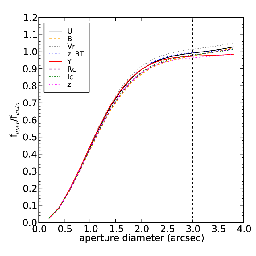
Figure 5: Mean growth curves for simulated point sources on the LBT and Subaru images. At least $96\%$ of the total flux is recovered at $3^{\prime\prime}$ aperture diameter.

In order to determine the flux lost when using a fixed aperture ( $\rm{3^{\prime\prime}}$), we include on the images, at random positions, simulated point sources with a PSF of ${1.06^{\prime\prime}}$ using the task ’mkobjects’ in IRAF. In Fig. 5 we present the growth curve for all the images. The flux lost is of the order of 0.05 in all cases. This is of the order of our accuracy and we choose not to add any corrections in the optical photometry.

The final photometric catalog is obtained by merging the detection on three images and at two detection thresholds, $\rm{5\sigma}$ and $\rm{3\sigma}$. The detection images are:

• Priority 1 – the Subaru Rc image. It is the best image in terms of seeing ($\rm{0.9^{\prime\prime}}$), depth ($\rm{R_{c,lim}=26.1\,mag}$), and area coverage ($\rm{0.53\,deg^{2}}$). We retrieve 160633 sources at the $\rm{5\sigma}$ detection level and 257352 sources at the $\rm{3\sigma}$ level.

• Priority 2 – the Subaru z’ image. There are sources detected in the z’ band which fall below the detection limit of the Rc band, due to their intrinsic SED. These objects could be high redshift galaxies and/or galaxies that have large amounts of dust. We choose to perform the detection on the Subaru over the LBT $\rm{z^{\prime}}$ image because it covers a larger area, it is deeper and it has better seeing. We retrieve 127362 sources at the $\rm{5\sigma}$ detection level and 250102 sources at the $\rm{3\sigma}$ level.

• Priority 3 – the LBT B image. With LBT the field has been observed with a sequence of short exposures which allowed to reach the same depth of Subaru but with less saturated sources. The number of sources we retrieve is 68107 at $\rm{5\sigma}$, while at $\rm{3\sigma}$ we retrieve 105658 sources.

In order to create the optical catalogs, we keep the whole Rc catalog and include from the z’ - and B - based catalogs, sources that are not present in the Rc catalog within $\rm{0.5^{\prime\prime}}$ from the Rc - sources. This is done for the $\rm{5\sigma}$ and $\rm{3\sigma}$ detection thresholds separately.

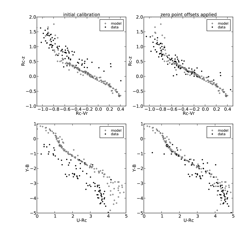
Figure 6: We used the star templates of Pickles (1998) to check for systematic offsets in the photometric calibration. Two examples of color-color plots of stars for models (open dots) and data (filled dots), before (left panels) and after (right panel) photometric correction are presented here.

As a consistency check of the photometric calibration and as cross calibration between different bands/telescopes, we compared theoretical colors of stars with the colors of star candidates from our catalog (Fig. 6). In this context, stars are those bright sources ($\rm{R_{c}<19}$) that SExtractor defines point-like ($\rm{R_{class}>0.98}$) by comparison with the PSF of the image. A more refined star/galaxy separation, on the basis of the SED fitting will be performed later on, in the final compilation of the catalog (see section 5.3).

After the comparison of the stellar photometry with the stellar tracks, a mean correction of the order of $\sim$0.1 mag is applied to the photometry with exception the Y band. As seen in Fig. 6, the Y band required a zero point offset of $\sim 0.8$. This was expected, as the zero point was only approximate, since no standard stars were observed during the Y band observations.

3.2.2 Combining Optical with Other Wavelengths

In order to merge our optical catalogs with the GALEX, SDSS, UKIDSS and IRAC catalogs, we proceed as follows (Fig. 4).

We associated all optical sources with the closest GALEX source within $\rm{1^{\prime\prime}}$. As the PSF of the GALEX images is much larger ($\rm{5^{\prime\prime}}$), a larger search radius should be adopted. However, as the publicly available GALEX catalog does not account for blended sources, a small radius reduces the number of false matches (see also Arnouts et al., 2005, for optical to GALEX associations). We retrieved $\sim 3700$ and $\sim 10000$ couterparts in FUV and NUV, respectively.

For the Sloan Catalog, the matching radius is reduced to $\rm{0.6^{\prime\prime}}$. This corresponds to 3 pixels on our optical images. We keep only the sources for which $\rm{r^{\prime}<22\,mag}$, similarly to the selection criterion of Oyaizu et al. (2008). We find approximately 5700 matches with the SDSS catalog.

For consistency, as we registered the optical images to the SWIRE coordinates, thus we registered the UKIDSS catalog to our grid. We found a systematic relative offset of about $\rm{0.2^{\prime\prime}}$, which has been corrected by changing the astrometry of the UKIDSS catalog using Aladin (Bonnarel et al., 2000). We then matched the optical and UKIDSS catalogs keeping the closest infrared source to the optical coordinates within a $\rm{0.6^{\prime\prime}}$ radius to compensate for any further astrometric differences. We found approximately 25000 matches between the optical and the UKIDSS sources. From these matches, $98\%$ lie inside a radius of $\rm{0.5^{\prime\prime}}$ from the optical position. Additionally $~{}650$ matches are located within a distance between $\rm{0.5^{\prime\prime}-0.6^{\prime\prime}}$ which corresponds to a physical distance of 2.5-3 pixels on our images.

Finally, we incorporated the Spitzer catalogs using positional matching within $\rm{1^{\prime\prime}}$ from the optical position. We are using a large matching radius for the same reasons as in the case of GALEX. Approximately 26000 sources are matched to an optical source.

In order to create the final merged catalog, we keep all the sources detected in the $\rm{5\sigma}$ level, and the sources detected in the $\rm{3\sigma}$ level which i) have a UKIDSS counterpart and ii) are not present within $0.5^{\prime\prime}$ from the sources in the $\rm{5\sigma}$ catalog. This choice is a compromise between sources of lower significance and false detections. In the catalog, we provide a flag denoting which catalog each source originates from. In addition, in order to account for problems originated by blending, we flag sources that are not isolated. The released catalog consists of 187611 sources and is described in detail in §3.2.5.

3.2.3 X-ray Sources and their properties

In the final catalog, sources that are identified as counterparts to the X-ray detections are flagged. The association in optical/near-infrared/mid-infrared bands using the maximum likelihood ratio technique is described in detail in (Rovilos et al., 2011). We include in the photometric catalog 389 out of the 409 X-ray detected sources in the field. The 20 sources not present are either too faint to be detected even at the $\rm{3\sigma}$ threshold or are associated with stars. For the sources flagged as X-ray detections we provide additional information that will be of crucial importance for the computation of photometric redshifts. These are the morphology and variability analysis.

Morphology

Recently, HST images became available for the central area of the XMM region (covering in total $0.034\;deg^{2}$, red circle in Fig. 1, PI: Somerville). We used those images to classify the counterparts of X-ray sources in i) point-like and ii) extended, by visual inspection. We also performed morphological classification by visual inspection of the B and Rc bands. The final morphology is assigned based primarily on the HST images, complemented by the ground based images for the sources with no HST coverage. We classified 134 sources as point-like and 140 as extended. From the remaining sources 103 are too faint to be classified and 12 are associated with saturated sources (see Table 3).

Variability

AGN vary on time scales from days to years. This intrinsic property complicates the computation of photometric redshifts. The photometry is most of the times gathered over many years and a change in flux can be misinterpreted as an emission line. The variability in COMBO 17 (Wolf et al., 2004) and in COSMOS (Salvato et al., 2009), was quantified through observations of the same energy band repeated over the years. The comparison of these repeated observations allowed the identification of the variable sources and the correction of the photometry. In the Lockman Hole, we can detect variability but we cannot correct for it. Thus, we limit the analysis in flagging the variable sources. The variability flag will serve as warning for potentially unreliable photometric redshifts.

We use as proxy of the variability the flux variation in the $\rm{z^{\prime}}$ band, for which we have observations from the Subaru telescope, from LBT and from SDSS. The variability is expected to be more significant for bright sources, as for fainter sources the photometric errors are large. Taking into account only bright sources ($\rm{18<z<22}$), we compute the variability ($Z_{var,k}$, $k=1,2,3$) and the associated error ($\delta Z_{var,k}$) for all three pairs of available $\rm{z^{\prime}}$ filters:

$$Z_{var,k}=z^{\prime}_{i}-z^{\prime}_{j}$$ (1)

and

$$\delta Z_{var,k}=\sqrt{(z^{\prime}_{err,i})^{2}+(z^{\prime}_{err,j})^{2}}$$ (2)

Using theoretical magnitudes of galaxies (see §4.1.1 for details), we verified that the expected deviation in the photometry, because of the slightly differing $\rm{z^{\prime}}$ filters, is always less than 0.2 magnitudes for redshifts up to 5.6, for all types of galaxies. Therefore, we flag a source as variable if $|Z_{var,k}\pm\delta Z_{var,k}|>0.2$ in at least one pair of the observations. We flag 102 sources as varying and 58 sources as non-varying. The remaining 229 sources, are either faint ($\rm{z>22}$) or they are lacking z-band photometry and they are treated as non-varying.

3.2.4 Spectroscopic sample

Compared to other fields, the number of spectroscopic redshift available in Lockman Hole is limited and focused mostly on AGN and infrared galaxies. From all the available catalogs (see Table 4 for a complete list), we extract the spectroscopic redshifts with the highest confidence. The quality is provided either by the authors (and in these cases we cannot verify the quality of the redshift estimate) or, when the spectrum is available, it is assessed by us. We define a redshift reliable when more than 1 feature (either in emission and/or in absorption) is present in the spectrum.

We are using 10 redshifts from Schmidt et al. (1998) (${0.245<z<2.144}$) and 50 redshifts from Lehmann et al. (2001) (${0.074<z<4.45}$), where the sources were observed as possible counterparts of the X-ray sources detected by ROSAT. Also, during the same observing run normal galaxies where observed as secondary targets. These observations were published in the PhD thesis of I. Lehmann (Universität Potsdam, 2000). In this way we recovered additional 29 reliable spectroscopic redshifts (${0.045<z<0.903}$).

Furthermore, we include the observations by Zappacosta et al. (2005) (${0.085<z<1.13}$), who studied the presence of a superstructure in the field. Their catalog contains 48 high quality spectroscopic redshifts, with the superstructure being at redshift $\sim 0.8$. We include 42 redshifts from the SDSS catalog (${0.00<z<3.269}$) and 44 redshifts retrieved from NASA/IPAC Extragalactic Database (NED) (${0.073<z<3.036}$).

Our group has also observed sources in the Lockman Hole Field. Focusing on the counterparts of XMM detected sources two observing runs were performed with KECK/DEIMOS between 2004 and 2007 (38 high quality redshift, $0.029<z<3.408$) and in 2010 (20 sources, $0.353<z<1.302$). Furthermore, spectroscopic follow up of the SWIRE field provided 321 high quality spectroscopic redshifts (Huang et al. in preparation) ($0.018<z<3.471$).

In total, we have 602 high quality spectroscopic redshifts, out of which 487 are redshifts of normal galaxies with median redshift of $z=0.42$ ($0.000<z<3.471$) with 252 galaxies being inside the XMM area. Furthermore, 115 correspond to X-ray detected sources with median redshift of $z=0.79$ ($0.024<z<4.45$).

3.2.5 Description of the Photometric Catalog

In the following we give a brief description of each column in the catalog. We adopt the value ”-99” for null fields inside the catalog. An excerpt of the catalog is presented in Tab. 5.

• ID – unique identification number for the final catalog.

• Optical coordinates (J2000) from the detection image – in addition we provide the coordinates of the counterparts in the GALEX, UKIDSS, SDSS, and IRAC catalogs.

• AB Magnitudes and errors – aperture photometry corrected to total (only for GALEX and IRAC photometry) for point-like sources and associated error for the filters: $\rm{FUV}$, $\rm{NUV}$, $\rm{U}$, $\rm{B}$, $\rm{V}$, $\rm{z^{\prime}_{LBT}}$, $\rm{Y}$, $\rm{R_{c}}$, $\rm{I_{c}}$, $\rm{z^{\prime}_{Subaru}}$, $\rm{u^{\prime}}$, $\rm{g^{\prime}}$, $\rm{r^{\prime}}$, $\rm{i^{\prime}}$, $\rm{z^{\prime}}$, $\rm{J}$, $\rm{K}$, $\rm{3.6\mu m}$, $\rm{4.5\mu m}$, $\rm{5.8\mu m}$, $\rm{8\mu m}$.

• Detection flags – the meaning of the flags is: 1 - Rc detection ($\rm{5\sigma}$), 2 - $\rm{z^{\prime}}$ detection ($\rm{5\sigma}$), 3 - B detection ($\rm{5\sigma}$), 4 - Rc detection ($\rm{3\sigma}$), 3 - $\rm{z^{\prime}}$ detection ($\rm{3\sigma}$), 6 - B detection ($\rm{3\sigma}$).

• Photometry flag – complementary to the flag provided by SExtractor indicating saturation, we masked problematic regions on the images which include bad pixels and problematic areas close to stars, using ’Weight Watcher’ (Marmo & Bertin, 2008). In Table 6 we describe the flag values which we provide for each band. For more details, refer to the associated description file of the catalog.

• Neighbor flag – sources that have a neighbor within $1.5^{\prime\prime}$ carry a flag 1, while sources without close by neighbors carry a flag 0.

• Star/galaxy classification – the classification provided by SExtractor (1 = star, 0 = galaxy), measured on the corresponding detection image.

• Spectroscopic redshift and reference – we use only the high quality spectroscopic redshifts from the original catalogs according to Table 4.

• Variability – sources with $|Z_{var,k}\pm\delta Z_{var,k}|>0.2$ carry a flag 1, while the rest carry a flag 0.

• X-ray detection – sources detected in the X-rays are flagged as 1, sources inside the XMM area without X-ray detection are flagged as 0, while sources outside the XMM area are flagged as -99.

• X-ray ID – the sources identified as X-ray counterparts will have the corresponding X-ray ID number from the XMM catalog (Brunner et al., 2008). The non X-ray detected sources have a value of XID=-99.

• Morphology – as discussed in detail in §3.2.3, this column gives the merged morphology classification information from the HST and ground based images, provided only for the counterparts of the X-ray sources. The flags used and their meaning are presented in detail in Table 3.

4 Photometric Redshifts

In this section we describe the configuration of the photometric redshift computation. This includes the SED templates, the extinction and redshift grid, the second order correction applied in the photometry as well as the special treatment of the X-ray sample. We also define the quantities we use later on in the discussion to assess the quality of the results.

4.1 LePhare Setup

We compute photometric redshifts for all the sources in the field, using the publicly available code, LePhare. The code performs least squares minimization to retrieve the best fitting template to the photometric data. In order to achieve the optimum result for both normal galaxies and AGN, we treated the samples separately and with different sets of templates and priors. In the following we describe the templates and the priors used in the two cases.

4.1.1 Templates

We decided to adopt the same templates as used by Ilbert et al. (2009); Salvato et al. (2009) in the COSMOS field. Being well tested with a large spectroscopic sample, the templates are now included by default in the distribution of the LePhare. We briefly summarize here their major characteristics.

For the normal galaxies the template set consists of elliptical (templ. no. 1-7), spiral (templ. no. 8-19) and starburst templates (templ. no. 20-31) (Ilbert et al. (2009), Fig. 1). Extinction according to the Small Magellanic Cloud (SMC) law (Prevot et al., 1984) is applied for templates Sb-SB3, while for the templates SB4-SB11 Calzetti (Calzetti et al., 2000) and modified Calzetti laws are applied. No additional extinction is applied for templates redder than Sb. The intrinsic galactic absorption is computed with values E(B-V) = 0.00, 0.05, 0.10, 0.15, 0.20, 0.25, 0.30, 0.40, 0.50. Finally, the templates are calculated at redshifts 0-6 with step $\Delta z=0.01$, and at redshifts 6-7 with step $\Delta z=0.2$. Emission lines are added to the templates as this has been proven to give better results even in the case of broadband photometry (Ilbert et al., 2009).

For the X-ray detected sample, we are using the same library used in Salvato et al. (2009, 2011) for computing the photometric redshifts of XMM-COSMOS and Chandra-COSMOS. The library includes normal galaxies, local AGN, and hybrid templates. The templates forming the library where chosen (and, in the case of the hybrids created) to represent the spectroscopic sample available for the XMM-COSMOS survey, as documented in Salvato et al. (2009). The SEDs of galaxies hosting an AGN and pure galaxy differ mostly in the ultra-violet where the contribution of the accretion disk is expected and in the infrared where the reprocessed AGN radiation by the torus surrounding the central black hole is dominant. The templates of pure AGN dominated sources are taken from the library of Polletta et al. (2007) and are characterized by a typical power-law spectrum. To the pure type 1 AGN, the power-law is extended to the UV beyond the Ly$\alpha$. The reason for it is that the templates are empirical and thus diminished in the UV by the absorbers along the line of sight. As LePhare accounts by default for this absorption, without the addition of the power-law, the templates would be absorbed twice. More details on the construction of the templates can be found in Salvato et al. (2009). We apply only the SMC extinction law with E(B-V) values of 0.00, 0.05, 0.10, 0.15, 0.20, 0.25, 0.30, 0.35, 0.40, 0.45, 0.50. The templates are calculated with the same redshift steps as in the case of normal galaxies.

All the sources of our catalog are also fit with stellar SEDs of F-K dwarfs and G-K giant stars (Pickles, 1998), white dwarfs (Bohlin et al., 1995), low mass stars (Chabrier et al., 2000) and sub-dwarfs Bixler et al. (1991).

4.1.2 Residual zero-point offsets

Systematic differences can be found between templates and observed SEDs, due to uncertainties in the templates and second order calibration problems in photometry. The impact of calculating and using these offsets on the accuracy of the result is demonstrated in Ilbert et al. (2006). With the option ’AUTO_ADAPT’ in LePhare we compute the average difference in magnitude between the photometry in a given band and the photometry for the best SED fitting at the fixed spectroscopic redshift of a sample of normal galaxies ($\rm{18<R_{c}<24}$, $\sim$260 sources). Iteratively, we then search for the best set of corrections that minimize the offsets. Once found, the offset is applied with the option ’APPLY_SYSSHIFT’ to the SEDs when computing photometric redshift for the entire catalog. The same offsets are also applied when computing the photometric redshift for the X-ray sources. The offsets are presented in Table 7, and they are not included in the photometry presented in the catalog. We do not calculate any offsets for the $\rm{5.8\mu m}$ and $\rm{8.0\mu m}$ filters of IRAC, due to the large uncertainties in the theoretical models in these wavelengths.

We also include an additional factor to the photometric errors in quadrature (optical $\rm{0.02\,mag}$, ultra-violet and infrared $\rm{0.2\,mag}$). This factor compensates for the underestimated errors provided by SExtractor (Becker et al., 2007; McCracken et al., 2001).

4.1.3 Photometric Redshift Computation

The separate treatment of the sources based on the X-ray detection and emission, allows a pre-selection of templates and luminosity priors that reduces the possible parametric space of the solutions lifting degeneracies between the templates and therefore reducing the number of wrong photometric redshift solutions. In Fig. 8 we present the flow chart for the proper separation of the sample, and the template - prior combination we adopt for this work.

First of all, the sample is separated in non - X-ray detected and X-ray detected sources. For the non - X-ray detected sample we use the templates for normal galaxies presented in Ilbert et al. (2009) with priors $-24<M_{B}<-8$, which is the typical range of the absolute B magnitude for normal galaxies. For the X-ray detected sources, a further separation is required between point-like or varying sources (QSOV) and extended and non-varying (EXTNV) sources. The QSOV sample contains the AGN dominated sources and for them we are using the AGN templates of Salvato et al. (2009) with the same priors $-30<M_{B}<-20$.

The EXTNV sample contains moderately AGN dominated sources, starburst and normal galaxies. As demonstrated in Salvato et al. (2011), AGN that are low X-ray emitters, extended and not varying are better fit by normal galaxy templates, even if the X-ray luminosity is above $\rm{10^{42}erg\cdot sec^{-1}}$. For this reason, we treat differently sources that above and below a threshold set at $\rm{F_{0.5-2\,keV}>8\cdot 10^{-15}erg\,cm^{-2}\,s^{-1}}$. Above this value, the sources are fitted by AGN templates. The library of normal galaxies defined by Ilbert et al. (2009) is used otherwise. In both cases, the luminosity prior $-24<M_{B}<-8$ is adopted. It is important to stress that the threshold was defined using a sample of 700 sources with spectra, belonging to the EXTNV group, in the COSMOS field.

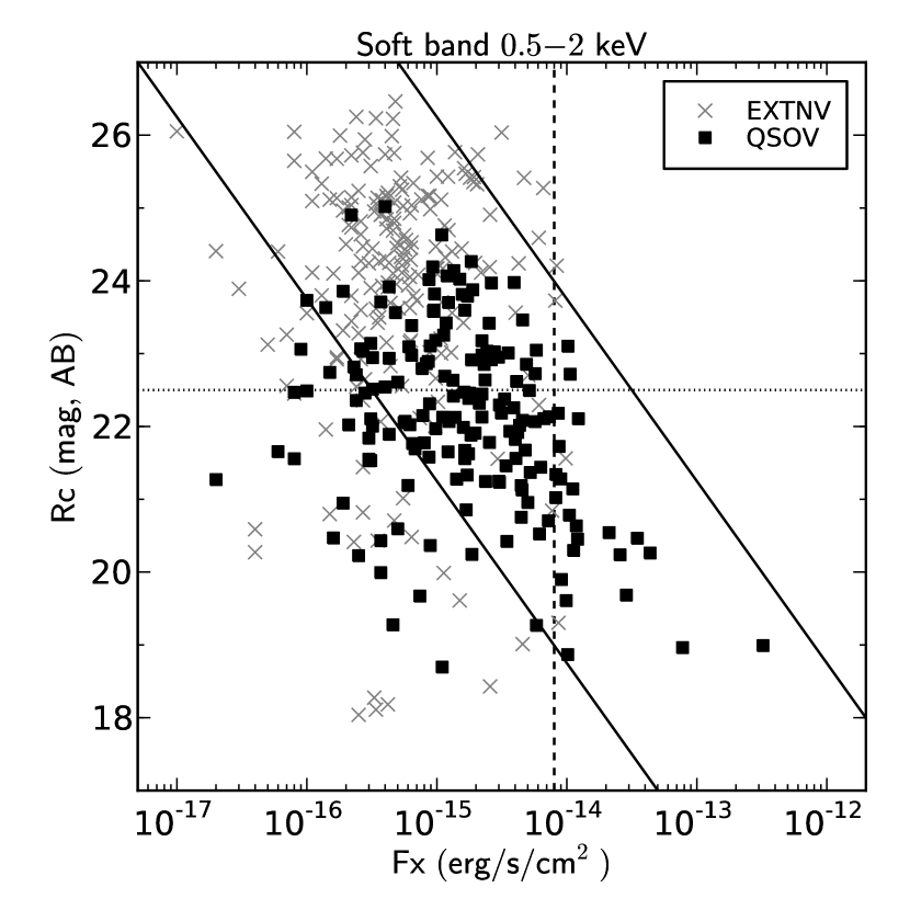
Figure 9: Rc magnitude versus soft X-ray flux $\rm{(0.5-2\,keV)}$. The crosses represent all the EXTNV sample and the squares the QSOV sample. The black solid lines correspond to $\rm{log(f_{X}/f_{R})\pm 1}$ where the majority of the AGNs lie. Non-active galaxies will be in the lower left region of the diagram. The vertical dashed line denotes the X-ray threshold we apply to the EXTNV sample for adopting different templates and priors. The horizontal line marks the bright subsample ($R_{c}<22.5$).

In Fig. 9 we plot the optical magnitude ($\rm{R_{c}}$) versus the soft X-ray flux ($\rm{0.5-2\,keV}$) for all the X-ray detected sources. The squares indicate sources in the QSOV sample and the crosses indicate sources in the EXTNV sample. The two black solid lines mark the area in which the majority of the AGN-dominated sources is found and they are defined as:

$$log{(\frac{f_{x}}{f_{Rc}})}=\pm 1$$ (3)

where,

$$log{(\frac{f_{x}}{f_{Rc}})}=log{f_{x}}+\frac{Rc}{2.5}+5.5$$ (4)

see also Maccacaro et al. (1988) Hornschemeier et al. (2003) and Brusa et al. (2005).

The separation of the sources in QSOV and EXTNV is purely based on morphological and variability considerations. Examining sources for which we can distinguish between point-like and extended morphology ($R_{c}<24$) we find that 76.4% of the QSOV sources are found in the area between the two solid black lines in Fig. 9, while 53.5% of the EXTNV sources are found in the same area, justifying our original assumption that QSOV sources are AGN-dominated sources and need to be treated with appropriate templates and luminosity priors.

Focusing on the bright ($Rc<22.5$, dotted line), extended, non varying sources, we see that the above mentioned empirical threshold in the X-rays (vertical dashed line at $\rm{F_{0.5-2keV}=8\cdot 10^{-15}erg\,s^{-1}\,cm^{-2}}$), separates efficiently the AGN dominated systems from starbursts and normal galaxies, which populate the lower left corner of this diagram (Hornschemeier et al., 2003). The positive improvement of the X-ray threshold when computing photometric redshifts for X-ray sources, is only marginal for this work, as the brighter sources are rare and the Lockman Hole is a small field. However, the threshold resulted in a noticeable improvement on the XMM-COSMOS surveys (Salvato et al., 2011) and we decided to adopt the same strategy for consistency.

4.2 Outlier-accuracy definition

Outliers

Since the photometric redshift computation is a multivariate problem with many degeneracies, is it bound to produce wrong solutions for some objects (see for discussion Richards et al. (2001)).

Comparing the photometric redshift solutions to the spectroscopic redshifts, we quantify the fraction of outliers $\eta$ as the ratio $100\cdot N_{out}/N_{total}$ where $N_{total}$ is the number of sources with spectroscopic redshift and $N_{out}$ the number of sources with:

$$\frac{|z_{phot}-z_{spec}|}{1+z_{spec}}>0.15$$ (5)

Accuracy

The accuracy of the photometric redshifts is usually quantified by the direct comparison of the photometric redshift solution against the spectroscopic value. In the literature there are many ways of computing the accuracy, from the pure root mean square (rms) of the $\Delta z=(z_{phot}-z_{spec})/(1+z_{spec})$, to the rms after 1 or 3 sigma clipping, depending on the authors (Wolf et al., 2004; Mobasher et al., 2004; Margoniner & Wittman, 2008; Dahlen et al., 2010).

Another more robust way to quantify the accuracy of the sample is to consider the median of the deviations from the true (spectroscopic) value. In this way the accuracy accounts also for the outliers. We adopted this approach, described in detail in Hoaglin et al. (1983) and used e.g. by Brammer et al. (2008); Wuyts et al. (2008); Ilbert et al. (2009); Salvato et al. (2009); Cardamone et al. (2010). The Normalized Median Absolute Deviation (NMAD) is defined as:

$$\sigma_{NMAD}=1.48\cdot median|\Delta z|$$ (6)

where $\Delta z=(z_{phot}-z_{spec})/(1+z_{spec})$. This quantity is expected to remain close to zero for all redshifts.

5 Results

5.1 Photometric Redshifts of normal galaxies

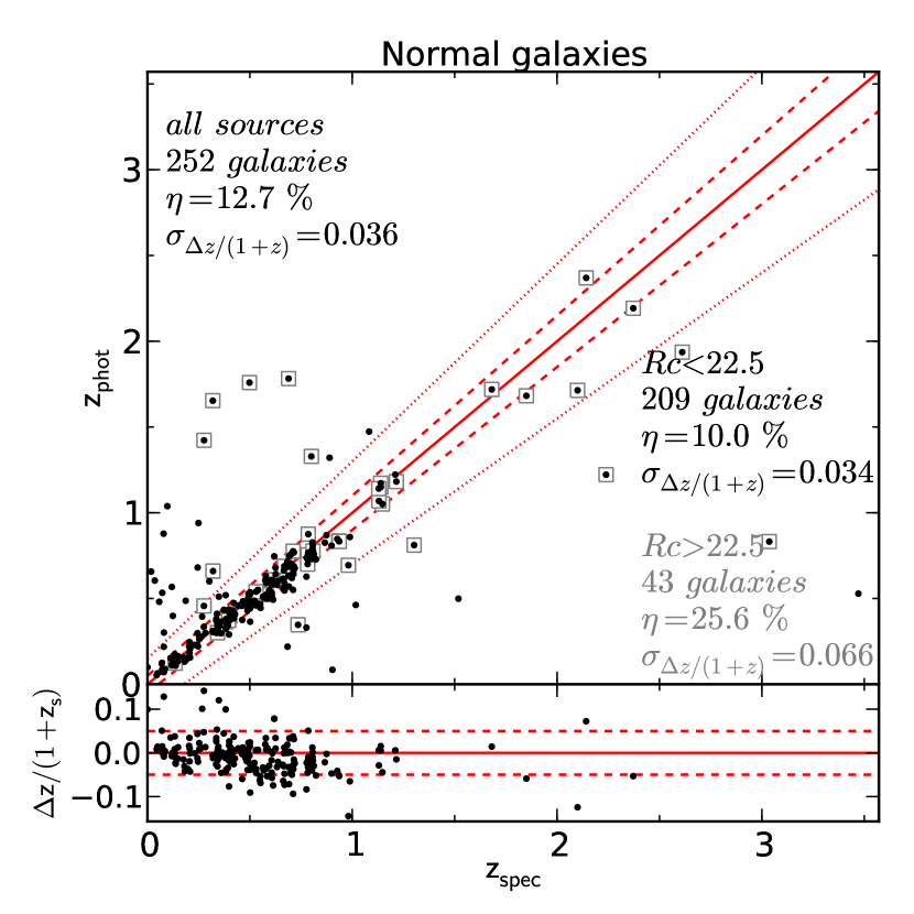
Figure 10: Photometric redshift versus spectroscopic redshift for the normal galaxies. With gray squares we denote the faint sources ($\rm{Rc>22.5\,mag}$). The solid line is the $\rm{z_{phot}=z_{spec}}$ relation. The dashed lines are $\rm{z_{phot}=0.05\pm(1+z_{spec})}$. The dotted lines are $\rm{z_{phot}=0.15\pm(1+z_{spec})}$. Sources that lie outside the dotted lines are defined as outliers.

We retrieve photometric redshift for 184642 non - X-ray detected sources in the Lockman Hole area with $45\%$ of them computed with at least six photometric bands. The remaining 1978 sources lack a photometric redshift solution since they have only two photometric bands available. In Fig. 10 we compare the photometric versus the spectroscopic redshifts. For the bright subsample ($\rm{Rc<22.5\,mag}$) the accuracy is $\sigma_{NMAD}=0.034$ (eq. 6) and the fraction of outliers $\eta=10.0\%$.

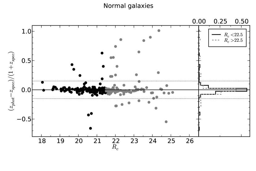
Figure 11: The ratio $\rm{(z_{phot}-z_{spec})/(1+z_{spec})}$ versus optical magnitude $\rm{R_{c}}$ for normal galaxies and corresponding histogram on the right panel. The photometric redshifts of bright sources ($\rm{R_{c}<22.5}$, black filled circles and black solid line) are mostly confined between $\rm{|(z_{phot}-z_{spec})/(1+z_{spec})|<0.15}$ (dotted lines, marking the outlier region), while the outliers with the largest discrepancies are faint sources ($\rm{R_{c}>22.5\,mag}$, gray open circles and gray dashed line).

Even though our photometric catalog does not contain medium or narrow band photometry, our result does not suffer from systematic biases. This is also clear in Fig. 11, where the ratio $(z_{phot}-z_{spec})/(1+z_{spec})$ is plotted as a function of optical magnitude. The distribution of the ratio $(z_{phot}-z_{spec})/(1+z_{spec})$ is centered at zero (histogram, right panel) both for bright ($R_{c}<22.5$, black solid line) and faint sources ($R_{c}>22.5$, gray dashed line). For the latter, however, the fraction of outliers is higher and consequently the accuracy decreases. This is a well known trend, discussed already by many other authors ( (e.g., Cardamone et al., 2010; Barro et al., 2011; Ilbert et al., 2009; Salvato et al., 2009); at fainter magnitudes the spectral energy distribution is less tightly constrained, and only by upper limits in some bands, or has large statistical uncertainties associated with the photometry.

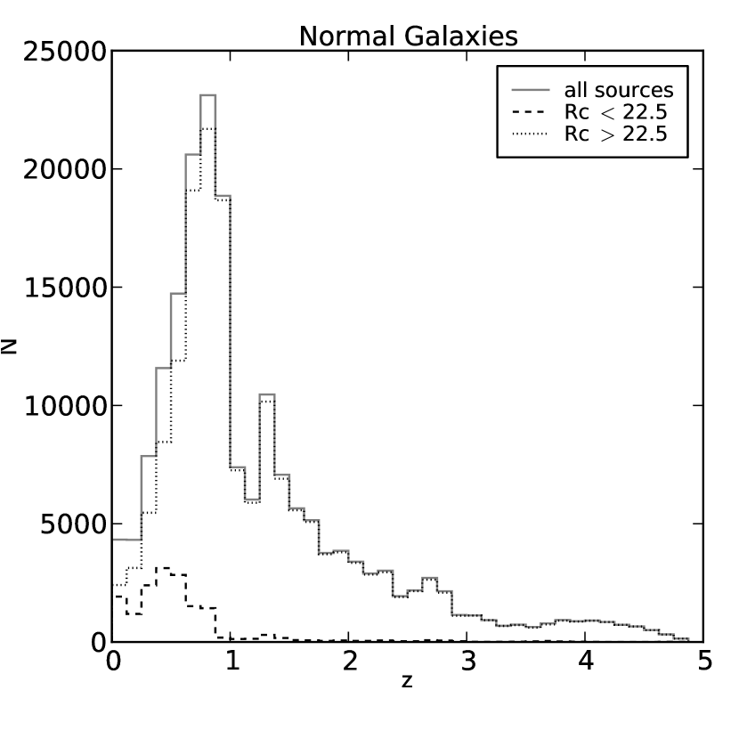
Figure 12: Redshift distribution for normal galaxies, using spectroscopic redshift when available. Bright galaxies ($\rm{R_{c}<22.5\,mag}$) lie mostly at redshift $z<1$.

In Table 8 we summarize the accuracy and the percentage of the outliers for various subsamples. The majority of the sources with spectra available have redshift $z_{\rm spec}<$1, and therefore we can characterize the quality of our redshift solutions, in a statistically robust way, only for low redshift sources. For $z_{\rm spec}<$1, the accuracy is $\sigma_{NMAD}=0.034$ (eq. 6) and the fraction of outliers is $\eta=9.6\%$. Fig. 12 shows the redshift distribution of the normal galaxies (solid line) separated in optically bright ($\rm{Rc<22.5\,mag}$, dashed line) and optically faint ($\rm{Rc>22.5\,mag}$, dotted line), where spectroscopic redshifts substitute photometric redshifts when possible.

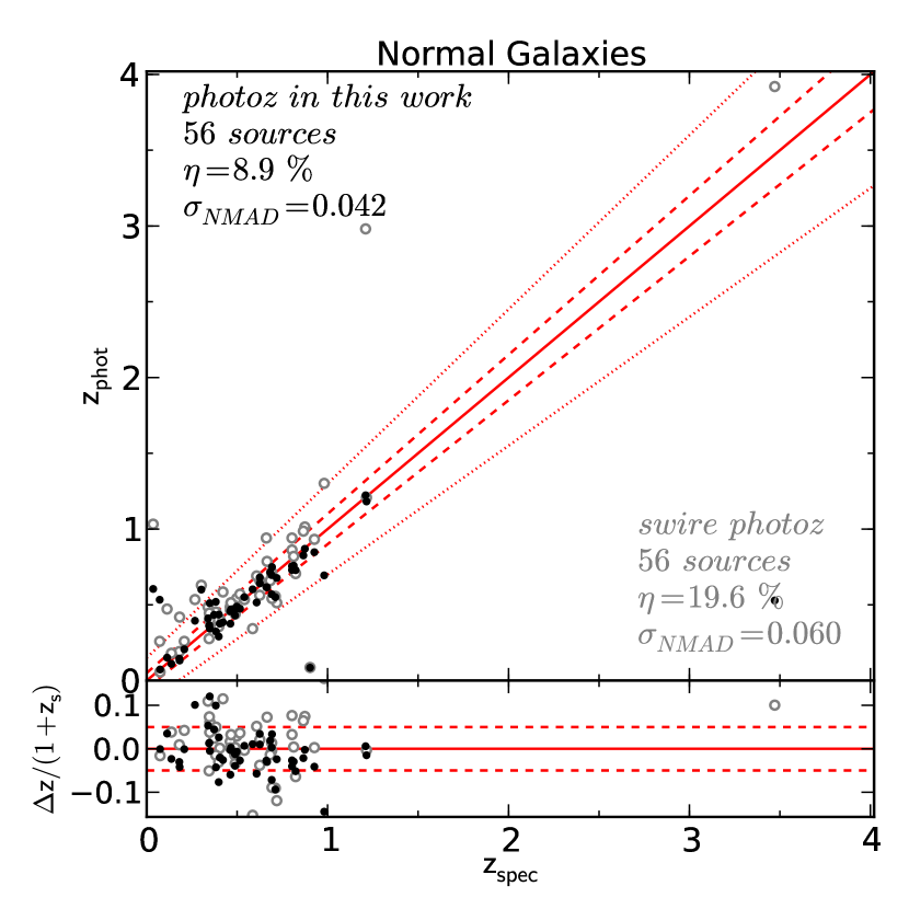
Figure 13: Comparing the quality of new photometric redshifts, using sources in common in the present work (black filled dots) and the SWIRE catalog (gray open circles). There is a dramatic decrease in the fraction of outliers and the accuracy is improved.

In Fig. 13 we also compare the photometric redshifts from this work with the previous available photometric redshifts available from (Rowan-Robinson et al., 2008). We consider only the sources in common to the two samples for which spectroscopic redshifts are available (56 sources). Due to the increased number of bands used in this work, we achieve an accuracy improved up to a factor of 1.5 for normal galaxies and 2 times less outliers.

5.2 Photometric redshifts of X-ray detected sources

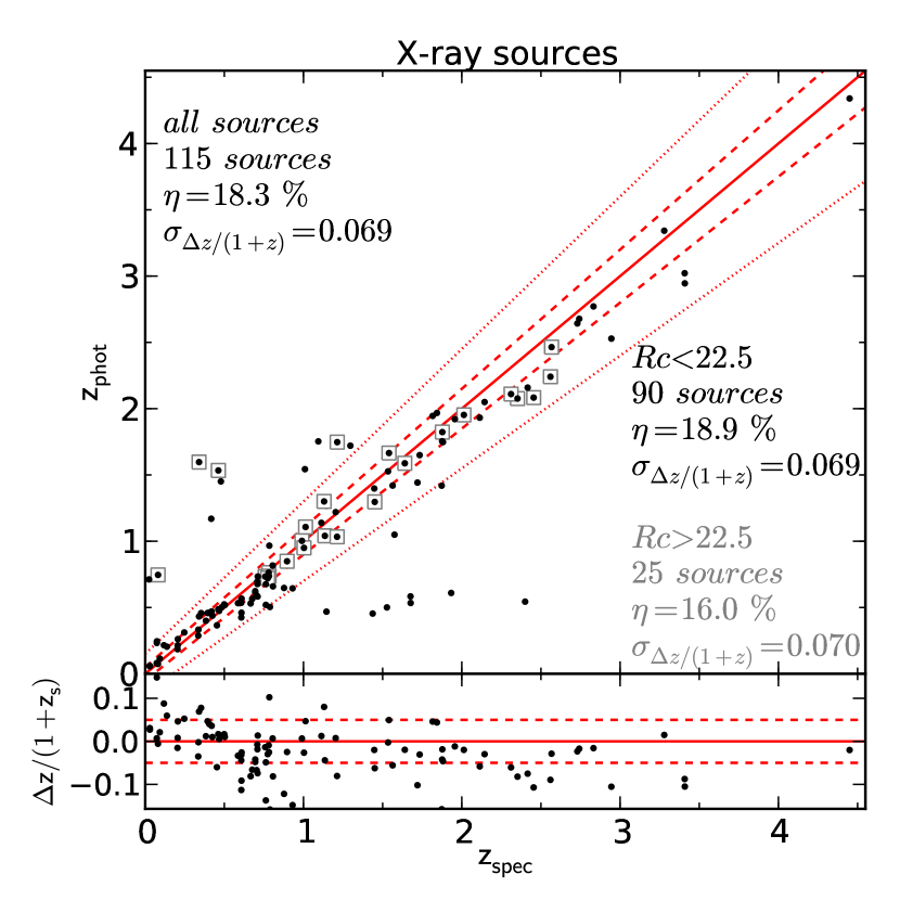
Figure 14: Photometric redshift versus spectroscopic redshift for the X-ray detected sources. The symbols and lines are the same as in Fig. 10.

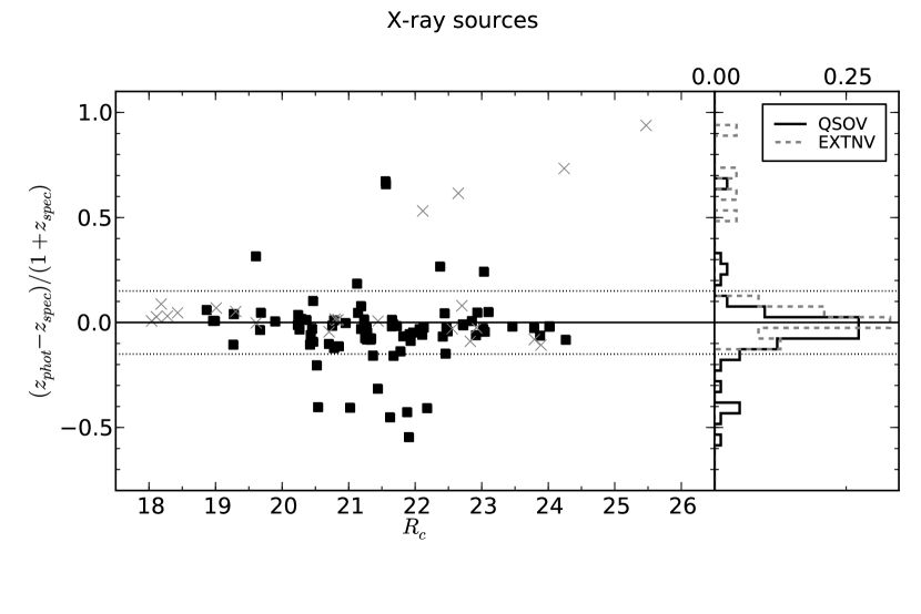
Figure 15: The ratio $\rm{(z_{phot}-z_{spec})/(1+z_{spec})}$ versus optical magnitude $\rm{R_{c}}$ for X-ray sources and corresponding histogram on the right panel. The squares denote the QSOV sample (point-like or varying sources) and the crosses denote the EXTNV sample (extended and not varying sources). The variability is a key factor in the photometric redshift computation, as 11 out of the 16 outliers belonging in the QSOV sample are identified as varying sources. As in the case of the normal galaxies, the largest discrepancies are found for faint sources ($\rm{R_{c}>22.5\,mag}$).

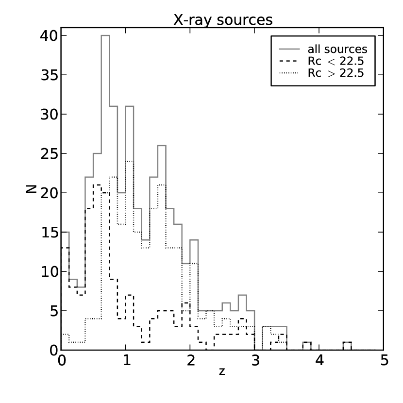
Figure 16: Redshift distribution of X-ray sources, using spectroscopic redshift when available.

For the counterparts of the X-ray sources, mostly AGN, the accuracy of the bright subsample is $\sigma_{NMAD}=0.069$, while the fraction of outliers is $\eta=18.9\%$ (Fig. 14). This is similar to the accuracy reached by XMM-COSMOS and Chandra-COSMOS when the same bands and depths available for Lockman Hole are considered, without correcting for variability. The impact of variability in our photometric redshift computation is shown in Fig. 15. Even thought the distribution of $(z_{\rm phot}-z_{\rm spec}/(1+z_{spec})$ is peaked around zero, there are some sources in the QSOV subsample (squares) that show quite large deviations. Indeed, 11 out of the 16 outliers are flagged as varying sources indicating once more the care that should be taken in planning photometric observations of AGN. In Table 9 we summarize our results separating them on the basis of the classification of the sources (either EXTNV or QSOV) and brightness . In Fig. 16 we present the histogram of the redshifts for the X-ray detected sources (solid line) separated in optically bright ($\rm{Rc<22.5\,mag}$, dashed line) and optically faint ($\rm{Rc>22.5\,mag}$, dotted line).

In Table 8 we give the detailed evaluation of our results, in direct comparison with the non X-ray detected sample. As it is expected, the photometric redshifts of the brightest sources are more accurate than the redshifts for the fainter sources. The highest accuracy is reached at $z<1$ with $\sigma_{NMAD}=0.066$ and fraction of outliers $\eta=16.4\%$.

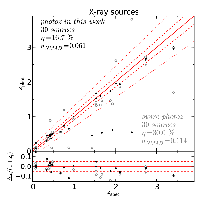
Figure 17: Comparison between previous photometric redshifts and results from this work for X-ray detected sources. The symbols are the same as in Fig. 13. As in the case of normal galaxies, the outliers are reduced significantly and the accuracy is improved.

In Fig. 17 we compare our results to the photometric redshifts of Rowan-Robinson et al. (2008). Apart from the increased number of used bands an additional reason for the improvement is that, contrary to Rowan-Robinson et al. (2008), our work was tuned to this kind of sources. Rather than adding AGN-dominated templates to the library of normal galaxies, we limited the degeneracies by using only AGN-dominated templates and appropriate priors, thus achieving more accurate results by a factor of 1.8 both in terms of accuracy and outliers.

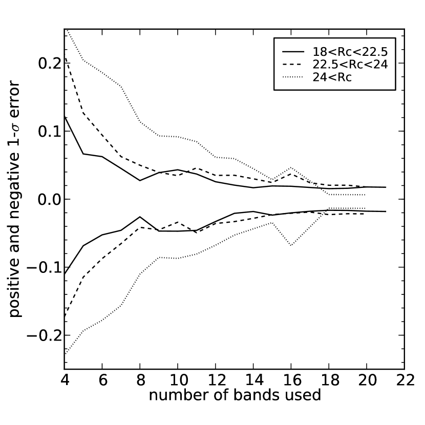
Figure 18: Mean error of photometric redshifts versus the number of bands used during the fitting. The bright sample (solid line) has a consistent behavior when six or more number of bands are used. The faint sample (dashed line) approaches the accuracy of the bright sample in cases when eight bands or more are available.

As already discussed, the accuracy of photometric redshifts correlates with the faintness of the sources. As a consequence, when the source is faint, less photometry is also available. In Fig. 18 we plot the median positive and negative $1-\sigma$ errors, defined as ($z_{best68,high}-z_{best}$) and ($z_{best}-z_{best68,low}$), per number of bands used in the SED fitting for all sources (non X-ray and X-ray detected sources). As expected, the bright sources show small errors even when using only a few bands, as bright sources have usually small errors associated with their photometry, thus making the least squares fitting more precise. We underline that narrow errors of photometric redshifts does not mean that the solution is the correct one, rather that the probability distribution has a narrow peak around a given value.

5.3 Star/galaxy separation

Rather than distinguishing between stars and galaxies, SExtractor separates the objects in point-like and extended. This is performed by comparison of the measured FWHM of an object with the PSF of the image (given as input), as a result the code is unable to distinguish between stars and unresolved galaxies.

To assess the limitations of SExtractor we compare the number of stars defined by the code, with the expected number of stars defined by stellar population synthesis models of galactic stars in the area covered by Lockman Hole. In the case of bright objects ($\rm{R_{c}}<19$) the number of stars detected by SExtractor (90 sources) agrees well with the expected number (103 sources). Inversely, in the case of less bright objects ($20<\rm{R_{c}}<22$) SExtractor classifies $\sim 1500$ sources as stars, almost three times more the number predicted by the simulation ($\sim 440$ stars), as it confuses point-like sources with unresolved ones.

At the same time, SED fitting can misclassify objects as stars especially in the case of elliptical galaxies that are lacking infrared photometry. To compensate between the two effects, we flag as stars sources that have been identified as stars both by SExtractor ($\rm{Classification}>0.95$) and by the SED fitting ($\rm{2\cdot\chi^{2}_{star}<\chi^{2}_{best}}$) using star templates from Pickles (1998); Bohlin et al. (1995); Chabrier et al. (2000); Bixler et al. (1991). With this conservative approach we flag $\sim 700$ sources as stars , excluding most of the false identifications. Indeed, according to the simulation we expect $\sim 800$ stars in the Lockman Hole area having the same magnitude distribution as the the sources identified as stars from the previous criterion.

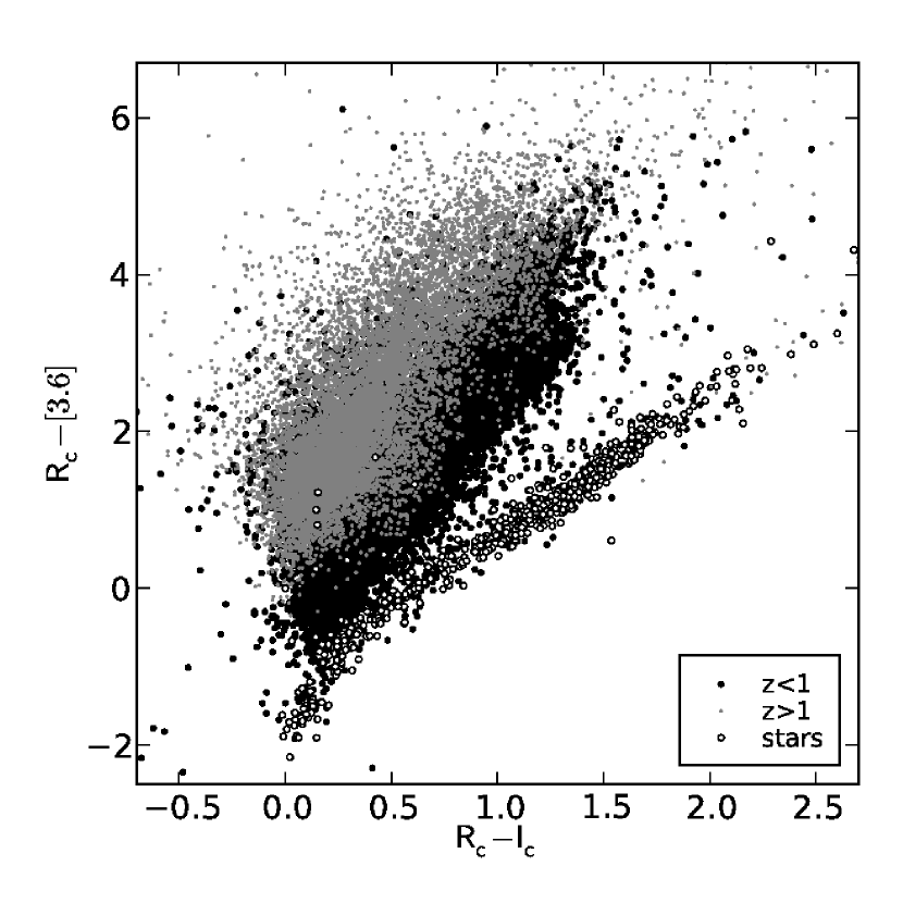
Figure 19: Color - color plot demonstrating the star - galaxy separation. Gray dots indicate high redshift galaxies, black circles low redshift galaxies and open circles indicate the stars. Most of the identified stars through the SED fitting, lie in the expected locus for stars.

Fig. 19 shows a color-color plot of stars (open circles), low redshift (black) and high redshift (gray) galaxies. With the combined criterion of morphology and SED fitting, we retrieve stars mainly in the expected locus according to theoretical templates (see also Ilbert et al. (2009)).

5.4 Description of the Photometric Redshift Catalog

In the following we give a description of the photometric redshift catalog, which we provide separately from the photometry catalog. An excerpt of the catalog is given in Tab. 10. The photometric redshift catalog includes:

• ID – corresponding identification number from the photometric catalog.

• $z_{best}$ – the best fitted solution for the photometric redshift.

• $z_{best68,low}$ – the lowest redshift at 68% significance.

• $z_{best68,high}$ – the highest redshift at 68% significance.

• $z_{best90,low}$ – the lowest redshift at 90% significance.

• $z_{best90,high}$ – the highest redshift at 90% significance.

• $\chi^{2}_{best}$ – the lowest $\chi^{2}$ value for the best fitted galaxy model.

• $PDZ_{best}$ – the probability that $z_{best}$ is the correct photometric redshift.

• $model_{best}$ – the number corresponding to the model best fitting the SED. 100+(1, …, 31) from Ilbert et al. (2009); 1, …, 30 from Salvato et al. (2009).

• $Ext-law_{best}$ – the extinction-law applied for computing $z_{best}$.

• $E(B-V)_{best}$ – the absorption applied for computing $z_{best}$.

• $Nband_{best}$ – number of bands used in the SED fitting.

• Similarly for the second photometric redshift solution, when available:

• $z_{sec}$ – the second best solution for the photometric redshift.

• $\chi^{2}_{sec}$ – the corresponding $\chi^{2}$ value .

• $PDZ_{sec}$ – the probability that the second $z_{best}$ is the correct photometric redshift.

• $model_{sec}$ – the number corresponding to the model best fitting the SED.

• $E(B-V)_{sec}$ – the absorption applied for computing the second $z_{best}$:

• $\chi^{2}_{star}$ – the lowest $\chi^{2}$ value for the best fitted star model.

• $Flag_{star}$ – we flag stars (1 = star, 0 = galaxy), as discussed in 5.3

6 Conclusions

We present and publicly release an optically based multiwavelength photometric catalog which contains 21 bands for sources detected in the Lockman Hole area. The catalog contains 187611 sources out of which 389 sources are associated with X-ray sources. The $50\%$ detection limits ($\rm{5\sigma}$) for the photometry are $\rm{R_{c}=26.1\,mag}$, $\rm{z^{\prime}=24.8\,mag}$ and $\rm{B=27\,mag}$. This is the first public catalog containing deep multiwavelength photometry for the Lockman Hole Deep Field.

Even though the lack of narrow/medium band photometry will affect studies that require detailed information of the SED of the source, the collection of broad-band photometric measurements we present here, can serve as a first educated guess of the shape of the SED, which we will address, focusing on the AGN in future work.

We also present and publicly release a complementary catalog with photometric redshift information for all sources. Depending on the nature of the sources (non X-ray and X-ray detected) we used different templates and priors, allowing a final accuracy for the bright subsample ($\rm{R_{c}<22.5\,mag}$) of $\sigma_{NMAD}=0.034$ with a fraction of $\rm{10\%}$ outliers for normal galaxies and $\sigma_{NMAD}=0.069$ with a fraction of $\rm{18.9\%}$ outliers for X-ray detected sources.

Figure 4: Schematic diagram of the merging procedure of the various catalogs. Using as base images the $\rm{R_{c}}$, $\rm{z^{\prime}}$, $\rm{B}$ images, we calculate in dual mode the photometry from the LBT and Subaru images. We perform positional matching with the independently obtained photometric catalogs from UKDISS, SDSS, IRAC, and GALEX. The X-ray catalog is then matched to the multi-wavelength optical catalog using Likelihood Ratio matching as described in Rovilos et al. (2011). A detailed description is given in §3.2.1.

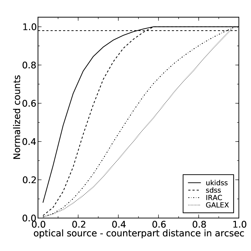
Figure 7: Cumulative curve of the distance between the optical position and the counterpart in the UKIDSS (solid line), SDSS (dashed line), IRAC (dot-dashed line), and GALEX (dotted line) catalog.

Figure 8: The flow chart describes the decision procedure for the optimum combination of templates and priors during the photometric redshift computation. The ’extnv’ sample contains the extended and the non-varying sources, while the ’qsov’ sample contains the point-like and varying sources. For this work, we adopt $\rm{F_{0.5-2keV}=8\cdot 10^{-15}erg\,s^{-1}\,cm^{-2}}$ as flux threshold to separate between X-ray bright and faint sources.

Table 1: Properties of recent X-ray fields sorted in decreasing area.

		Average	Number	Flux limit				X-ray
Field	Area	Exposure	of					point source
	($\rm{deg^{2}}$)	(ks)	sources	$0.5-2\rm{keV}$	$2-8\rm{keV}$	$2-10\rm{keV}$	$5-10\rm{keV}$	catalog
XMM-COSMOS	2.13	60	1887	$1.7\cdot 10^{-15}$	-	$9.3\cdot 10^{-15}$	$1.3\cdot 10^{-14}$	Cappelluti et al. (2007)
Chandra-COSMOS	0.9	200	1761	$1.9\cdot 10^{-16}$	-	$7.3\cdot 10^{-16}$		Elvis et al. (2009)
AEGIS	0.67	200	1325	$5.3\cdot 10^{-17}$	-	$3.8\cdot 10^{-16}$	-	Laird et al. (2009)
ECDFS	0.3	250	762	$1.1\cdot 10^{-16}$	$6.7\cdot 10^{-16}$	-	-	Lehmer et al. (2005)
Lockman Hole	0.2	185	409	$\mathbf{1.9\cdot 10^{-16}}$	-	$\mathbf{9\cdot 10^{-16}}$	$\mathbf{1.8\cdot 10^{-15}}$	Brunner et al. (2008)
CDFN	0.124	1000	503	$2.7\cdot 10^{-17}$	$1.4\cdot 10^{-16}$	-	-	Alexander et al. (2003)
CDFS	0.129	2000	740	$9.1\cdot 10^{-18}$	$5.5\cdot 10^{-17}$	-	-	Xue et al. (2011)

Table 2: Observational facts for the ground-based observations

	Large Binocular Telescope						Subaru
	U	B	V	z’	Y		Rc	Ic	z’
Area ($\rm{deg^{2}}$)	0.26	0.25	0.19	0.20	0.19		0.53	0.53	0.53
Filter $\rm{\lambda_{eff}(\AA)}$	3573	4249	5405	9050	9880		6518	7957	9064
Filter FWHM ($\rm{\AA}$)	540	916	845	1053	465		1167	1381	1154
Exposure (sec)	49680	19972	9540	14400	10980		3920	6235	10400
PSF FWHM (′′)	1.06	0.90	0.95	1.06	0.60		0.90	0.98	0.96
Limiting Magnitude (5$\sigma$, AB)	26.7	27.0	26.7	24.2	23.5		26.1	25.5	24.8
AB correction	0.964	-0.046	-0.005	0.528	0.558		0.207	0.436	0.521

Table 3: Morphology’s flag description

		Number of Sources
Description	Flag	HST	Ground based	Final morphology
too faint / unresolved source	-20	44	86	103
photometry blended with nearby source	-10	5	10	12
extended source	+00	20	151	140
point-like source	+10	23	123	134

Table 4: Spectroscopic redshift reference

Flag	reference
1	Lehmann et al. (2001)
2	Lehmann, PhD Thesis, Potsdam (2000)
3	unpublished redshift KECK/DEIMOS (2004-2007)
4	unpublished redshift KECK/DEIMOS (2010)
5	SDSS DR2
6	Zappacosta et al. (2005)
7	Chapman et al. (2005)
8	Schmidt et al. (1998)
9	Swinbank et al. (2004)
10	Chapman et al. (2004)
11	Hainline et al. (2009)
12	Barris et al. (2004)
13	Stevens et al. (2003)
14	Mainieri et al. (2002)
15	Rodighiero et al. (2005)
16	Oyabu et al. (2005)
17	Mateos et al. (2005)
18	Hasinger et al. (1998)
19	Ishisaki et al. (2001)
20	Smail et al. (2004)
21	Ciliegi et al. (2003)
22	Hashimoto et al. (2005)
23	Ivison et al. (2005)
24	Fadda et al. (2002)
25	Huang et al. (in preparation)
26	Afonso et al. (2011))

Table 5: Lockman Hole Photometric catalog

ID	ra	dec	mag	mag	mag	neigh	classification	zspec	zspec	var	XMM	XMMNR	morphology
				err	flag	flag			cat		detection
134555	162.5407563	57.64900553	25.6317	0.057156	1	0	0.40040278	-99.0	-99	-99	-99	-99	-99
144534	162.5407569	57.70602821	24.6622	0.03174	0	0	0.5890769	-99.0	-99	-99	-99	-99	-99
43512	162.5407670	57.12902011	25.3024	0.062409	0	0	0.37800178	-99.0	-99	-99	-99	-99	-99
40455	162.5407798	57.11082514	20.6579	0.00478	0	0	0.4363798	-99.0	-99	-99	-99	-99	-99
41535	162.5407868	57.11838781	25.1448	0.052445	0	0	0.5059889	-99.0	-99	-99	-99	-99	-99

Table 6: Photometry’s flag description

Flag	Description
-99	99 value produced by SExtractor either for
	the magnitude or the error,
	or source outside of the field
-5	flag in the UKIDSS catalog
	marking noise in the JHK bands
-4	saturation or incomplete/corrupted data
	produced by SExtractor
-3	source inside a stripe, as marked by optical
	inspection of the images
-2	magnitude error was negative
-1	magnitude error was greater than 1
+0	everything is OK
+1	FWHM in the detection band is zero
+2	source inside wings of stars, potentially fake
+3	magnitude greater than the detection limit

Table 7: Offsets between theoretical templates and observations

Filter	Offset
FUV (GALEX)	-0.165
NUV (GALEX)	-0.356
U (LBT)	0.125
B (LBT)	-0.026
V (LBT)	-0.038
z’ (LBT)	-0.054
Y (LBT)	0.141
$\rm{R_{c}}$ (Subaru)	-0.037
$\rm{I_{c}}$ (Subaru)	-0.020
z’ (Subaru)	-0.004
u’ (SDSS)	0.271
g’ (SDSS)	-0.115
r’ (SDSS)	0.006
i’ (SDSS)	0.104
z’ (SDSS)	0.083
J (UKIRT)	0.249
K (UKIRT)	0.294
$\rm{3.6\mu m}$ (IRAC)	0.203
$\rm{4.5\mu m}$ (IRAC)	0.346

Table 8: Photometric redshift accuracy

	Non X-ray sources				X-ray sources
	N(zspec)	$\sigma$	$\eta(\%)$		N(zspec)	$\sigma$	$\eta(\%)$
all sources	252	0.036	12.7		115	0.069	18.3
$R_{c}<22.5$	209	0.034	10.0		90	0.069	18.9
$R_{c}>22.5$	43	0.066	25.6		25	0.070	16.0
$0<z<1$	230	0.034	9.6		67	0.066	16.4
$1.0<z<5$	22	0.146	45.5		48	0.078	20.8

Table 9: Detailed photometric redshift accuracy for the X-ray detected sample

	QSOV				EXTNV
	N(zspec)	$\sigma$	$\eta(\%)$		N(zspec)	$\sigma$	$\eta(\%)$
all sources	85	0.071	18.8		30	0.056	16.7
$R_{c}<22.5$	70	0.084	21.4		20	0.036	10
$R_{c}>22.5$	15	0.042	6.7		10	0.126	30.0

Table 10: Lockman Hole Photometric Redshift catalog

IDENT	Z_BEST	Z_BEST68	Z_BEST68	Z_BEST90	Z_BEST90	CHI	PDZ	MOD	EXTLAW	EBV	NBAND	Z	CHI	PDZ	MOD	EBV	CHI	STAR
		LOW	HIGH	LOW	HIGH	BEST	BEST	BEST	BEST	BEST	USED	SEC	SEC	SEC	SEC	SEC	STAR	FLAG
134555	1.6691	0.57	1.98	0.48	2.36	2.16843	42.222	31	0	0.0	3	0.63	2.80791	16.042	31	0.0	0.660721	0
144534	0.7756	0.76	0.79	0.73	0.8	92.5442	88.25	13	1	0.4	3	1.49	97.5873	6.911	4	0.0	53.7372	0
43512	1.6959	1.63	1.92	0.21	2.18	11.0777	55.532	31	0	0.0	3	0.26	12.1607	6.116	31	0.0	5.50912	0
40455	0.381	0.32	0.44	0.31	0.44	0.0459227	99.976	30	2	0.2	3	-99.0	1.0E9	0.0	-999	-99.0	133.076	0
41535	1.3348	0.34	1.39	0.33	1.45	6.26825	59.054	26	0	0.0	3	0.36	6.96524	21.341	31	0.4	14.71	0

References

- Abazajian et al. (2009) Abazajian, K. N., et al. 2009, ApJS, 182, 543
- Afonso et al. (2011) Afonso, J., Bizzocchi, L., Ibar, E., et al. 2011, arXiv:1108.4037
- Aird et al. (2010) Aird, J., et al. 2010, MNRAS, 401, 2531
- Alexander et al. (2003) Alexander, D. M., et al. 2003, AJ, 126, 539
- Arnouts et al. (2005) Arnouts, S., Schiminovich, D., Ilbert, O., et al. 2005, ApJ, 619, L43
- Barger et al. (2003) Barger, A. J., et al. 2003, AJ, 126, 632
- Barger et al. (2005) Barger, A. J., Cowie, L. L., Mushotzky, R. F., et al. 2005, AJ, 129, 578
- Barris et al. (2004) Barris, B. J., et al. 2004, ApJ, 602, 571
- Barro et al. (2011) Barro, G., Pérez-González, P. G., Gallego, J., et al. 2011, ApJS, 193, 30
- Becker et al. (2007) Becker, A. C., Silvestri, N. M., Owen, R. E., Ivezić, Ž., & Lupton, R. H. 2007, PASP, 119, 1462
- Bender et al. (2001) Bender, R., Appenzeller, I., Böhm, A., et al. 2001, Deep Fields, 96
- Bertin & Arnouts (1996) Bertin, E., & Arnouts, S. 1996, A&AS, 117, 393
- Bixler et al. (1991) Bixler, J. V., Bowyer, S., & Laget, M. 1991, A&A, 250, 370
- Bohlin et al. (1995) Bohlin, R. C., Colina, L., & Finley, D. S. 1995, AJ, 110, 1316
- Bonnarel et al. (2000) Bonnarel, F., et al. 2000, A&AS, 143, 33
- Brammer et al. (2008) Brammer, G. B., van Dokkum, P. G., & Coppi, P. 2008, ApJ, 686, 1503
- Brunner et al. (2008) Brunner, H., Cappelluti, N., Hasinger, G., Barcons, X., Fabian, A. C., Mainieri, V., & Szokoly, G. 2008, A&A, 479, 283
- Brusa et al. (2005) Brusa, M., et al. 2005, A&A, 432, 69
- Brusa et al. (2009) Brusa, M., Comastri, A., Gilli, R., et al. 2009, ApJ, 693, 8
- Bruzual & Charlot (2003) Bruzual, G., & Charlot, S. 2003, MNRAS, 344, 1000
- Budavári et al. (2000) Budavári, T., Szalay, A. S., Connolly, A. J., Csabai, I., & Dickinson, M. 2000, AJ, 120, 1588
- Calzetti et al. (2000) Calzetti, D., Armus, L., Bohlin, R. C., Kinney, A. L., Koornneef, J., & Storchi-Bergmann, T. 2000, ApJ, 533, 682
- Cappelluti et al. (2007) Cappelluti, N., et al. 2007, ApJS, 172, 341
- Caputi et al. (2006) Caputi, K. I., McLure, R. J., Dunlop, J. S., Cirasuolo, M., & Schael, A. M. 2006, MNRAS, 366, 609
- Cardamone et al. (2010) Cardamone, C. N., et al. 2010, ApJS, 189, 270
- Casali et al. (2007) Casali, M., et al. 2007, A&A, 467, 777
- Chabrier et al. (2000) Chabrier, G., Baraffe, I., Allard, F., & Hauschildt, P. 2000, ApJ, 542, 464
- Chapman et al. (2004) Chapman, S. C., Smail, I., Blain, A. W., & Ivison, R. J. 2004, ApJ, 614, 671
- Chapman et al. (2005) Chapman, S. C., Blain, A. W., Smail, I., & Ivison, R. J. 2005, ApJ, 622, 772
- Ciliegi et al. (2003) Ciliegi, P., Zamorani, G., Hasinger, G., Lehmann, I., Szokoly, G., & Wilson, G. 2003, A&A, 398, 901 G. H., Pérez-González, P. G., Rigby, J. R., & Alonso-Herrero, A. 2007, Deepest Astronomical Surveys, 380, 119
- Civano et al. (2011) Civano, F., Brusa, M., Comastri, A., et al. 2011, arXiv:1103.2570
- Dahlen et al. (2010) Dahlen, T., Mobasher, B., Dickinson, M., et al. 2010, ApJ, 724, 425
- Ebrero et al. (2009) Ebrero, J., Carrera, F. J., Page, M. J., et al. 2009, A&A, 493, 55
- Egami et al. (2004) Egami, E., et al. 2004, ApJS, 154, 130
- Elvis et al. (2009) Elvis, M., et al. 2009, ApJS, 184, 158
- Fadda et al. (2002) Fadda, D., Flores, H., Hasinger, G., Franceschini, A., Altieri, B., Cesarsky, C. J., Elbaz, D., & Ferrando, P. 2002, A&A, 383, 838
- Fiore et al. (2009) Fiore, F., et al. 2009, ApJ, 693, 447
- Gabasch et al. (2004) Gabasch, A., Bender, R., Seitz, S., et al. 2004, A&A, 421, 41
- Gabasch et al. (2006) Gabasch, A., Hopp, U., Feulner, G., et al. 2006, A&A, 448, 101
- Geach et al. (2011) Geach, J. E., Murphy, D. N. A., & Bower, R. G. 2011, MNRAS, 413, 3059
- Giodini et al. (2009) Giodini, S., et al. 2009, ApJ, 703, 982
- Hainline et al. (2009) Hainline, L. J., Blain, A. W., Smail, I., Frayer, D. T., Chapman, S. C., Ivison, R. J., & Alexander, D. M. 2009, ApJ, 699, 1610
- Hashimoto et al. (2005) Hashimoto, Y., Henry, J. P., Hasinger, G., Szokoly, G., & Schmidt, M. 2005, A&A, 439, 29
- Hasinger et al. (1998) Hasinger, G., et al. 1998, A&A, 340, L27
- Hasinger et al. (2005) Hasinger, G., Miyaji, T., & Schmidt, M. 2005, A&A, 441, 417
- Hewett et al. (2006) Hewett, P. C., Warren, S. J., Leggett, S. K., & Hodgkin, S. T. 2006, MNRAS, 367, 454
- Hoaglin et al. (1983) Hoaglin, D. C., Mosteller, F., & Tukey, J. W. 1983, Wiley Series in Probability and Mathematical Statistics, New York: Wiley, 1983, edited by Hoaglin, David C.; Mosteller, Frederick; Tukey, John W. Hernquist, L., Cox, T. J., & Kereš, D. 2008, ApJS, 175, 356
- Hodgkin et al. (2009) Hodgkin, S. T., Irwin, M. J., Hewett, P. C., & Warren, S. J. 2009, MNRAS, 394, 675
- Hornschemeier et al. (2003) Hornschemeier, A. E., et al. 2003, AJ, 126, 575
- Ilbert et al. (2006) Ilbert, O., Lauger, S., Tresse, L., et al. 2006, A&A, 453, 809
- Ilbert et al. (2006) Ilbert, O., et al. 2006, A&A, 457, 841
- Ilbert et al. (2009) Ilbert, O., et al. 2009, ApJ, 690, 1236
- Ishisaki et al. (2001) Ishisaki, Y., Ueda, Y., Yamashita, A., Ohashi, T., Lehmann, I., & Hasinger, G. 2001, PASJ, 53, 445
- Ivison et al. (2005) Ivison, R. J., et al. 2005, MNRAS, 364, 1025
- Laird et al. (2009) Laird, E. S., et al. 2009, ApJS, 180, 102
- Lawrence et al. (2007) Lawrence, A., et al. 2007, MNRAS, 379, 1599
- Lehmann et al. (2001) Lehmann, I., et al. 2001, A&A, 371, 833
- Lehmer et al. (2005) Lehmer, B. D., et al. 2005, ApJS, 161, 21
- Lockman et al. (1986) Lockman, F. J., Jahoda, K., & McCammon, D. 1986, ApJ, 302, 432
- Lonsdale et al. (2003) Lonsdale, C. J., et al. 2003, PASP, 115, 897
- Luo et al. (2010) Luo, B., Brandt, W. N., Xue, Y. Q., et al. 2010, ApJS, 187, 560
- Luo et al. (2011) Luo, B., Brandt, W. N., Xue, Y. Q., et al. 2011, arXiv:1107.3148
- Maccacaro et al. (1988) Maccacaro, T., Gioia, I. M., Wolter, A., Zamorani, G., & Stocke, J. T. 1988, ApJ, 326, 680 al. 1998, AJ, 115, 2285
- Mainieri et al. (2002) Mainieri, V., Bergeron, J., Hasinger, G., Lehmann, I., Rosati, P., Schmidt, M., Szokoly, G., & Della Ceca, R. 2002, A&A, 393, 425
- Mateos et al. (2005) Mateos, S., Barcons, X., Carrera, F. J., Ceballos, M. T., Hasinger, G., Lehmann, I., Fabian, A. C., & Streblyanska, A. 2005, A&A, 444, 79
- Margoniner & Wittman (2008) Margoniner, V. E., & Wittman, D. M. 2008, ApJ, 679, 31
- Marmo & Bertin (2008) Marmo, C., & Bertin, E. 2008, Astronomical Data Analysis Software and Systems XVII, 394, 619
- Massey et al. (2007) Massey, R., Rhodes, J., Ellis, R., et al. 2007, Nature, 445, 286
- McCracken et al. (2001) McCracken, H. J., Le Fèvre, O., Brodwin, M., et al. 2001, A&A, 376, 756
- Mobasher et al. (2004) Mobasher, B., Idzi, R., Benítez, N., et al. 2004, ApJ, 600, L167
- Morrissey et al. (2007) Morrissey, P., et al. 2007, ApJS, 173, 682
- Oke & Gunn (1983) Oke, J. B., & Gunn, J. E. 1983, ApJ, 266, 713
- Oyabu et al. (2005) Oyabu, S., et al. 2005, AJ, 130, 2019
- Oyaizu et al. (2008) Oyaizu, H., Lima, M., Cunha, C. E., Lin, H., Frieman, J., & Sheldon, E. S. 2008, ApJ, 674, 768
- Papovich et al. (2010) Papovich, C., Momcheva, I., Willmer, C. N. A., et al. 2010, ApJ, 716, 1503
- Pérez-González et al. (2008) Pérez-González, P. G., et al. 2008, ApJ, 675, 234
- Pickles (1998) Pickles, A. J. 1998, PASP, 110, 863
- Polletta et al. (2007) Polletta, M., et al. 2007, ApJ, 663, 81
- Prevot et al. (1984) Prevot, M. L., Lequeux, J., Prevot, L., Maurice, E., & Rocca-Volmerange, B. 1984, A&A, 132, 389
- Richards et al. (2001) Richards, G. T., et al. 2001, AJ, 122, 1151
- Rodighiero et al. (2005) Rodighiero, G., Fadda, D., Franceschini, A., & Lari, C. 2005, MNRAS, 357, 449
- Rovilos et al. (2009) Rovilos, E., et al. 2009, A&A, 507, 195
- Rovilos et al. (2011) Rovilos, E., Fotopoulou, S., Salvato, M., Burwitz, V., Egami, E., Hasinger, G., & Szokoly, G. 2011, arXiv:1102.5129
- Rowan-Robinson et al. (2008) Rowan-Robinson, M., et al. 2008, MNRAS, 386, 697
- Salvato et al. (2009) Salvato, M., et al. 2009, ApJ, 690, 1250
- Salvato et al. (2011) Salvato, M., Ilbert, O., Hasinger, G., et al. 2011, arXiv:1108.6061
- Schlegel et al. (1998) Schlegel, D. J., Finkbeiner, D. P., & Davis, M. 1998, ApJ, 500, 525
- Schmidt et al. (1998) Schmidt, M., et al. 1998, A&A, 329, 495 Trümper, J., & Zamorani, G. 1998, AJ, 115, 1230
- Smail et al. (2004) Smail, I., Chapman, S. C., Blain, A. W., & Ivison, R. J. 2004, ApJ, 616, 71
- Stevens et al. (2003) Stevens, J. A., Page, M. J., Ivison, R. J., Smail, I., Lehmann, I., Hasinger, G., & Szokoly, G. 2003, MNRAS, 342, 249
- Surace et al. (2005) Surace, J. A., Shupe, D. L., Fang, F., Evans, T., Alexov, A., Frayer, D., Lonsdale, C. J., & SWIRE Team 2005, Bulletin of the American Astronomical Society, 37, 1246
- Swinbank et al. (2004) Swinbank, A. M., Smail, I., Chapman, S. C., Blain, A. W., Ivison, R. J., & Keel, W. C. 2004, ApJ, 617, 64
- Taylor (2005) Taylor, M. B. 2005, Astronomical Data Analysis Software and Systems XIV, 347, 29
- Taylor (2006) Taylor, M. B. 2006, Astronomical Data Analysis Software and Systems XV, 351, 666
- Wolf et al. (2004) Wolf, C., Meisenheimer, K., Kleinheinrich, M., et al. 2004, A&A, 421, 913
- Wuyts et al. (2008) Wuyts, S., Labbé, I., Schreiber, N. M. F., et al. 2008, ApJ, 682, 985
- Xue et al. (2011) Xue, Y. Q., Luo, B., Brandt, W. N., et al. 2011, ApJS, 195, 10
- Zappacosta et al. (2005) Zappacosta, L., Maiolino, R., Finoguenov, A., Mannucci, F., Gilli, R., & Ferrara, A. 2005, A&A, 434, 801