Noisy-chaotic time series and
the forbidden/missing patterns paradigm

Abstract

We deal here with the issue of determinism versus randomness in time series. One wishes to identify their relative importance in a given time series. To this end we extend i) the use of ordinal patterns-based probability distribution functions associated to a time series [Bandt and Pompe, Phys. Rev. Lett. 88 (2002) 174102] and ii) the so-called Amigó paradigm of forbidden/missing patterns [Amigó, Zambrano, Sanjuán, Europhys. Lett. 79 (2007) 50001], to analyze deterministic finite time series contaminated with strong additive noises of different correlation-degree. Insights pertaining to the deterministic component of the original time series are obtained with the help of the causal entropy-complexity plane [Rosso et al. Phys. Rev. Lett. 99 (2007) 154102].

PACS: 05.45.Tp; 02.50.-r; 05.40.-a; 05.40.Ca; Version: V14

1 Introduction

1.1 Preliminaries

The distinction between deterministic and random components in time series has attracted considerable attention. From previous research, we may mention here work by A. R. Osborne and A. Provenzale [1], G. Sugihara and R. May [2], D. T. Kaplan and L. Glass [3, 4]. In particular, Kantz and co-workers [5, 6] analyzed recently the behavior of entropy quantifiers as a function of coarse-graining resolution, and applied their ideas to the issue of trying to distinguish between chaos and noise. Why is this an important issue? Due to the concept of deterministic chaos, derived from the modern theory of nonlinear dynamical systems, has profoundly changed our thinking on time-series analysis. Emphasis is being placed on non-linear approaches, i.e., dealing with nonlinear deterministic autonomous equations of motion representative of chaotic systems that give birth to irregular signals [7].

Clearly, signals emerging from chaotic time series occupy a intermediate position between (a) predictable regular or quasi-periodic signals and, (b) totally irregular stochastic signals (noise) that are completely unpredictable. However, they exhibit interesting phase-space structures. Chaotic systems display “sensitivity to initial conditions” which are the origin of instability everywhere in phase-space. This implies that instability uncovers information about the phase-space “population”, not available otherwise [8]. In turn this leads us to think of chaos as an information source, whose associated rate of generated-information is formulated in precise fashion via the Kolmogorov-Sinai’s entropy [9, 10]. These considerations motivate our present interest in the computation of quantifiers based on Information Theory, like, “entropy”, “statistical complexity”, “entropy-complexity plane”, etc. These quantifiers can be used to detect determinism in time series [11]. Indeed, different Information Theory based measures (normalized Shannon entropy and statistical complexity) allow for a better distinction between deterministic chaotic and stochastic dynamics whenever “causal” information is incorporated via the Bandt and Pompe’s (BP) methodology [12].

1.2 A new paradigm: forbidden patterns

When nonlinear dynamics are involved, a deterministic system can generate “random-looking” results that nevertheless exhibit persistent trends, cycles (both periodic and non-periodic) and long-term correlations. Our main interest here, lies in the emergence of “forbidden/missing patterns” [13, 14, 15, 16, 17]. Why? Because they have the potential ability for distinguishing deterministic behavior (chaos) from randomness in finite time series contaminated with observational white noise [13, 14, 17]. A concomitant helpful feature, as will be further explained below, is the decay rate of “missing ordinal patterns” as a function of the time series length.

In fact, Zanin [18] and Zunino et al. [19] have recently studied the appearance of missing ordinal patterns in financial time series. The presence of missing ordinal patterns has also been recently construed as evidence of deterministic dynamics in epileptic states. Ouyang et al. [20] found that a missing patterns’ quantifier could be used as a predictor of epileptic absence-seizures. It is essential to point out those works have only considered the presence of uncorrelated noise (white noise), which makes the associated results somewhat incomplete, since the presence of colored noise might be of importance. A first step in such direction was recently trodden by us in [21]. We pursue matters here by investigating the robustness of an associated mathematical construct called the causal entropy-complexity plane [11], that plays a prominent role in some of the above cited discoveries. We intend to do this by analyzing the planes’s ability to distinguish between noiseless chaotic time series and the ones that are contaminated (weekly to very strongly) with additive correlated noise. The chaotic series studied here were generated by recourse to a logistic map to which noise with varying amplitudes was added.

1.3 Organization of the paper

Our basic tools are 1) The MPR-statistical complexity measure together with entropic quantifiers, 2) The Bandt-Pompe approach to extract causal probability distributions functions (PDFs) from a given time-series, and 3) the construction of an entropy-complexity plane. These subjects are covered in great detail in [17, 21, 22]. For completeness, some details are given in the Appendix. The reader unfamiliar with these themes is strongly advised to go to the Appendix at this point. The forthcoming Section 2 details the problem to be discussed, while Section 3 revisits the Amigó paradigm. Our results are presented and discussed in Section 4, while some conclusions are drawn in Section 5. Background materials are provided in the Appendix.

2 Logistic map plus observational noise

The logistic map constitutes a canonic example, often employed to illustrate new concepts and/or methods for the analysis of dynamical systems. Here we will use the logistic map with additive correlated noise in order to exemplify the behavior of the normalized Shannon entropy ${\mathcal{H}}_{S}$ and the MPR-complexity ${\mathcal{C}}_{JS}$, both evaluated using a PDF based on the Bandt-Pompe’s procedure. We will also investigate the behavior of “missing ordinal patterns” in both a) the logistic map with additive noise (observational noise) and b) a pure-noise series, where the number of time series data was fixed at $N$.

The logistic map is a polynomial mapping of degree 2, $F:x_{n}\rightarrow x_{n+1}$ [23], described by the ecologically motivated, dissipative system represented by the first-order difference equation

$$x_{n+1}=r\cdot x_{n}\cdot(1-x_{n})\ ,$$ (1)

with $0\leq x_{n}\leq 1$ and $0\leq r\leq 4$.

Let $\eta^{(k)}$ be a correlated noise with $f^{-k}$ power spectra generated as described in [11, 21]. The steps to be followed are enumerated below.

1. Using the Mersenne twister generator [24] through the $\textsc{Matlab}^{\copyright}$ rand function we generate pseudo random numbers $y^{0}_{i}$ in the interval $(-0.5,0.5)$ with an (a) almost flat power spectra (PS), (b) uniform PDF, and (c) zero mean value.

2. The Fast Fourier Transform (FFT) ${y^{1}_{i}}$ is first obtained and then multiplied by $f^{-k/2}$, yielding ${y^{2}_{i}}$. Then, ${y^{2}_{i}}$ is symmetrized so as to obtain a real function. Subsequently the pertinent inverse FFT is found, after discarding the small imaginary components produced by the numerical approximations. The resulting noisy time series is then re-scaled to the interval $[-1,1]$, which produces a new time series $\eta^{(k)}$ that exhibits the desired power spectra and, by construction, is representative of non-Gaussian noises.

We consider time series of the form $\mathcal{S}=\{S_{n},n=1,\cdots,N\}$ generated by the discrete system:

$$S_{n}=x_{n}+A\cdot\eta^{(k)}_{n}\ ,$$ (2)

in which, $x_{n}$ is given by the logistic map and $\eta^{(k)}_{n}\in[-1,1]$ represents a noise with power spectrum $f^{-k}$ and amplitude $A$.

In generating the logistic map’s component of our time-series we fix $r=4$ and start the iteration procedure with a random initial condition. The first $5\cdot 10^{4}$ iterations are considered part of the transient behavior and discarded. After the transient part dies out, $N=10^{5}$ values are generated. In the case of the stochastic component of our time-series we consider $0\leq k\leq 2$ with $k$-values changing by an amount $\Delta k=1$ (other intermediate values have been considered in [21]). The noise amplitude was varied in order to cover different regimes from weak (the noise can be consider as perturbation to the logistic) to very strong (the logistic is consider a perturbation to the noise). Ten noisy time-series of length $N=10^{5}$ values and using different seeds, are generated for each value of the $k$-exponent.

3 The Amigó-paradigm

We arrive at the central point of our discussion. For deterministic one dimensional maps, Amigó et al. [13, 14, 15, 16] have conclusively shown that not all the possible ordinal patterns (as defined using Bandt and Pompe’s methodology, see Appendix) can be effectively materialized into orbits, which in a sense makes these patterns “forbidden”. We insist: this is an established fact, not a conjecture. The existence of these forbidden ordinal patterns becomes a persistent feature, a “new” dynamical property. For a fixed pattern-length (embedding dimension $D$) the number of forbidden patterns of a time series (unobserved patterns) is independent of the series length $N$. It must be noted, that this independence does not characterize other properties of the series such as proximity and correlation, which die out with time [14, 16]. For example, in the time series generated by the logistic map $x_{k+1}=4x_{k}(1-x_{k})$, if we consider patterns of length $D=3$, the pattern $\{2,1,0\}$ is forbidden. That is, the pattern $x_{k+2}<x_{k+1}<x_{k}$ never appears [14].

Stochastic processes could also have forbidden patterns [21]. However, in the case of uncorrelated (white noise) or certain correlated stochastic processes (noise with power low spectrum $f^{-k}$ with $k\geq 0$, ordinal Brownian motion, fractional Brownian motion, and fractional Gaussian noise), it can be numerically shown that no forbidden patterns emerge. In the case of time series generated by an unconstrained stochastic process (uncorrelated process) every ordinal pattern has the same probability of appearance [13, 14, 15, 16]. If the time series is long enough, all the ordinal patterns should eventually appear. If the number of time-series’ observations is sufficiently big, the associated probability distribution function should be the uniform distribution, and the number of observed patterns should depend only on the length $N$ of the time series under study.

For correlated stochastic processes the probability of observing individual patterns depends not only on the time series length $N$ but also on the correlation structure [17]. The existence of a non-observed ordinal pattern does not qualify it as “forbidden”, only as “missing”, and is due to the finite length of the time series. A similar observation also holds for the case of real data series, as they always possess a stochastic component due to the omnipresence of dynamical noise [25, 26, 27]. The existence of “missing ordinal patterns” could be either related to stochastic processes (correlated or uncorrelated) or to deterministic noisy processes, which is the case for observational time series.

3.1 The Carpi-Amigó test

Amigó and co-workers [13, 14] proposed a test that uses missing ordinal patterns to distinguish determinism (chaos) from pure randomness in finite time series contaminated with observational white noise (uncorrelated noise). The concomitant methodology [14] involves a graphic comparison between:

• The decay rate of the missing ordinal patterns (of length $D$) of the time series under analysis as a function of the series length $N$, and

• the decay rate exhibited by white Gaussian noise.

This methodology was recently extended by Carpi et al. [17] for the analysis of missing ordinal patterns in stochastic processes with different degrees of correlation. We are speaking of fractional Brownian motion (fBm), fractional Gaussian noise (fGn), and noises with $f^{-k}$ power spectrum (PS) and $k\geq 0$. Results show that for a fixed pattern length, the decay rate of missing ordinal patterns in stochastic processes depends not only on the series length but also on their correlation structures. In other words, missing ordinal patterns are more persistent in the time series with higher correlation structures. Carpi et al. [17] have also shown that the standard deviation of the estimated decay rate of missing ordinal patterns ($\alpha$) decreases with increasing $D$. This is due to the fact that longer patterns contain more temporal information and are therefore more effective in capturing the dynamic of time series with correlation structures.

An important quantity for us, called ${\mathcal{M}}(N,D)$, is the number of missing ordinal patterns of length $D$ not observed in a time series with $N$ values. As we mentioned before, for pure correlated stochastic processes the probability of observing an individual pattern of length $D$ depends on the time series-length $N$ and on the correlation structure (as determined by the type of noise $k>0$ ). In fact, as established for noises with an $f^{-k}$ PS in [17], as the value of $k>0$ augments – which implies that correlations grow – increasing values of $N$ are needed in reaching the “ideal” condition ${\mathcal{M}}(N,D)=0$. If the time series is chaotic but has an additive stochastic component, then one expects that as the time series’ length $N$ increases, the number of “missing ordinal patterns” will decrease and eventually vanish. That this may happen does not only depend on the length $N$ and on the underlying deterministic components of the time series but also on the correlation-structure of the added noise.

4 Present results

We wish to analyze and characterize the behavior of finite, noisy and chaotic time-series by recourse to patterns generated in the (causal) entropy-complexity plane. We intend to assess in particular the planar-geography of the forbidden patterns. The focus of attention is centered upon the roles of i) the noise amplitude $A$ and ii) the type of contaminating noise (degree of correlation). We consider noises with $f^{-k}$-power spectrum.

For our present analysis, we fix the pattern-length at $D=6$, the embedding time lag at $\tau=1$, and the time series length at $N=10^{5}$ values. For each one of the ten time series series generated (see Eq. (2)) and for each pair $(A,k)$, the normalized Shannon entropy ${\mathcal{H}}_{S}$ and the MPR-statistical complexity ${\mathcal{C}}_{JS}$ were evaluated using the Bandt and Pompe PDFs. We deal with additive (observational) noise with $k=0,1,$ and $2$, and analyze their position (each point results from an average over 10 different series) in the ${\mathcal{H}}\times{\mathcal{C}}$-planar graphs. A previous study has extensively dealt with the subject, but only in a special scenario in which the noise is of perturbative character [21]. Here we deal with the behavior of $(A,k)$ in the planar-graphs way beyond the perturbative $A$-zone, by considering also $A>1$ values.

4.1 Case $0\leq A\leq 1$

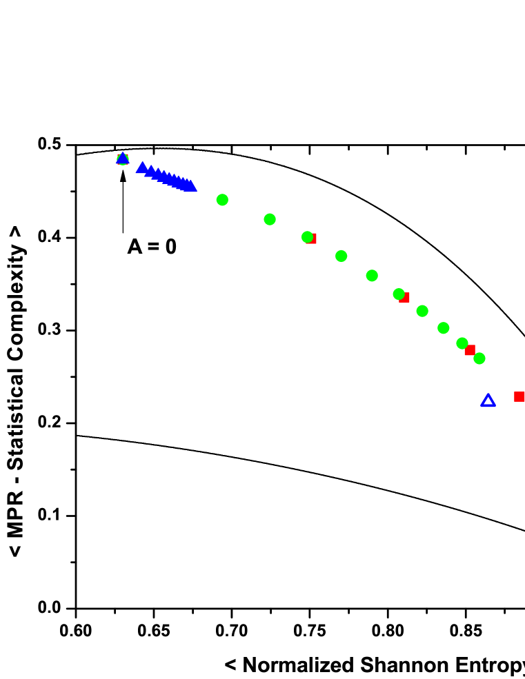
Figure 1: The causality entropy-complexity plane for all time series values (mean) corresponding to noise amplitude $0\leq A\leq 1$ ($\Delta A=0.1$) and $k=0,1,2$. Values for strictly noisy time series are also shown as open symbols. The values shown were obtained from times series of length $N=10^{5}$, and Bandt-Pompe parameters $D=6$, $\tau=1$. The lines represent the values of minimum and maximum statistical complexity ${\mathcal{C}}_{min}$ and ${\mathcal{C}}_{max}$ evaluated for the case of pattern length $D=6$.

Figure 1 summarizes the planar behavior of the noisy chaotic time series considered (the logistic map with additive correlated noise with $f^{-k}$ PS), considering noise amplitudes $0\leq A\leq 1$ ($\Delta A=0.1$) and $k=0$ (uncorrelated), $k=1,2$ (correlated), see also Fig. 8 in [21]. Clearly, given the noise-amplitude values here considered, the noise has a mere perturbative role vis-a-vis of the logistic map’s chaotic behavior.

For $A=0$ we obtain the purely deterministic value corresponding to the logistic time-series, localized approximately at a medium-high entropic coordinate, near the highest possible complexity value. Note that such is the typical behavior observed for deterministic systems [11]. For a purely uncorrelated stochastic process ($k=0$) we have ${\mathcal{H}}_{S}=1$ and ${\mathcal{C}}_{JS}=0$. The correlated (colored) stochastic processes ($k\neq 0$) yield points located at intermediate values between the curves ${\mathcal{C}}_{min}$ and ${\mathcal{C}}_{max}$, with decreasing values of entropy and increasing values of complexity as $k$ grows [11] (see Fig. 1, open symbols). From this figure and, also from our previous work [21], we see that if $k\approx 0$, for increasing values of the amplitude $A$, entropy and complexity values change (starting from the value corresponding to the pure logistic series, i.e., $A=0$) with a tendency to approach the values corresponding to pure noise, that is, (${\mathcal{H}}_{S}\approx 1$ and ${\mathcal{C}}_{JS}\approx 0$). Similar behavior is observed when correlated noises are considered, $k\neq 0$.

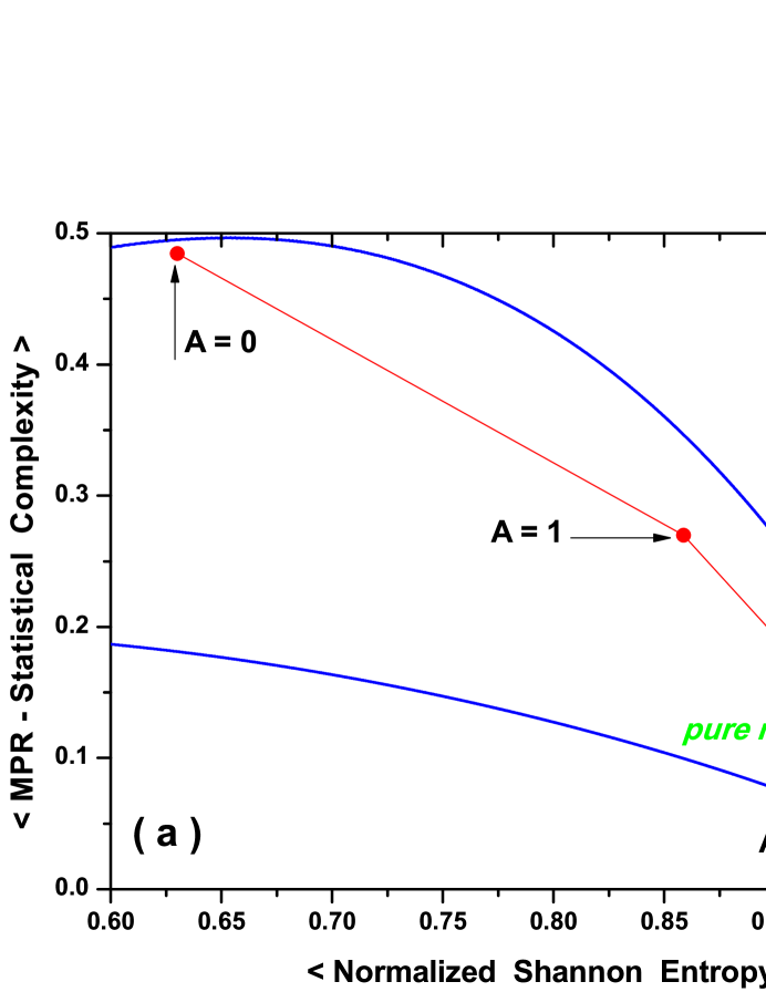
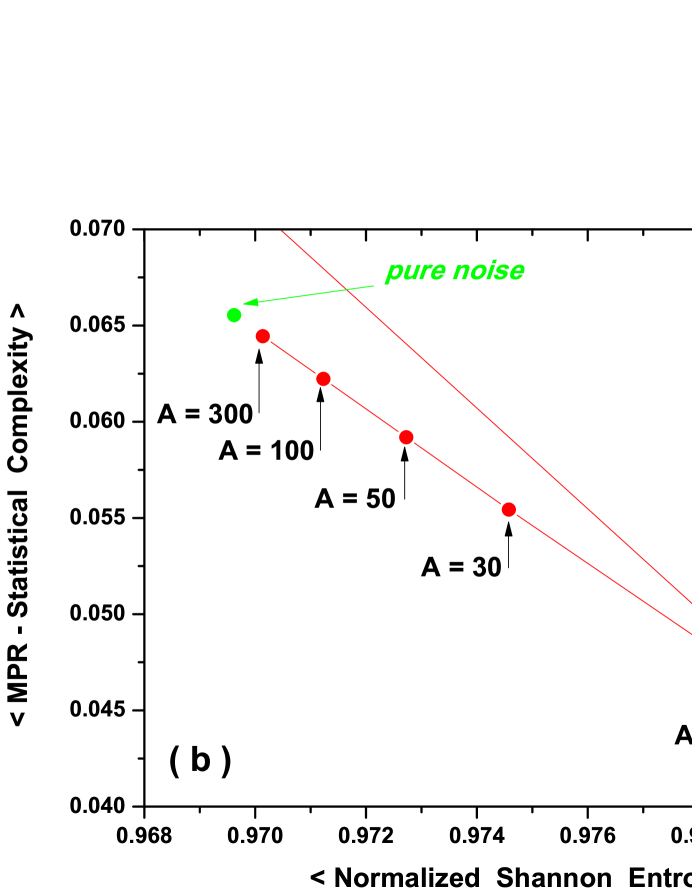
Figure 4: a) The causality entropy-complexity plane for all time series values (mean) corresponding to increasing values of noise amplitude $A$ and $k=1$. Value for the case of strictly noisy time series is shown as open symbol. The values shown were obtained from times series of length $N=10^{5}$, and Bandt-Pompe parameters $D=6$, $\tau=1$. The lines represent the values of minimum and maximum statistical complexity ${\mathcal{C}}_{min}$ and ${\mathcal{C}}_{max}$ evaluated for the case of pattern length $D=6$. b) Detail for high entropy values.

The main effect of the additive noise ($A\neq 0$) is to shift the point representative of zero noise ($A=0$) towards increasing values of entropy ${\mathcal{H}}_{S}$ and decreasing values of complexity ${\mathcal{C}}_{JS}$. This shift defines a kind of “trajectory” (curve) in the ${\mathcal{H}}\times{\mathcal{C}}$-plane, that is located in the vicinity of the maximum complexity ${\mathcal{C}}_{max}-$curve. Moreover, we found (by looking at other chaotic maps) that this trajectory is characteristic of the dynamical system under analysis. Such behavior can be linked to the persistence of forbidden patterns because they, in turn, imply that the deterministic logistic component is still operative and influencing the time series’ behavior [21]. As $k$ increases, the dependence on the noise-amplitude $A$ ($0\leq A\leq 1$) tends to become attenuated, implying that ${\mathcal{M}}(N,D)\neq 0$ (see Fig. 4 of [21]), while it almost disappears for $k\approx 2$. This fact is due to the effect of the “coloring” correlations of the noise, that grow with increasing values of $k$.

4.2 Case $A\geq 1$

Here we are interested in the physics associated to $A$’s growth, entailing an interchange between the roles of the logistic map and of the noise because a large $A$ makes noise the dominant feature. Several effects should be considered

• noise contamination level (represented by $A$),

• noise correlation (represented by $k$) and,

• persistence of the forbidden patterns.

We should expect that as $A$ grows (with fixed values for $N$ and $D$), the missing-patterns numbers would diminish and eventually vanish. With strong or very strong noise we expect zero missing patterns and eventual predominance of stochastic features. This means ${\mathcal{M}}(N,D)=0$ independently of the $A$ value. However, taking into account our previous results [21], we expect that some new specific features will be revealed by the use of the causality entropy-complexity plane.

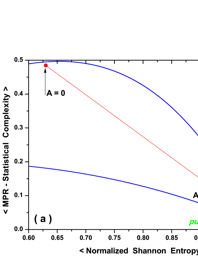
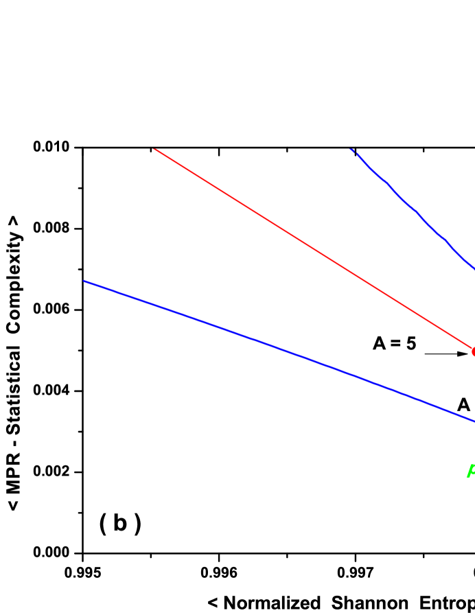
Figure 2: a ) The causality entropy-complexity plane for all time series values (mean) corresponding to increasing values of noise amplitude $A$ and $k=0$. Value for the case of strictly noisy time series is shown as open symbol. The values shown were obtained from times series of length $N=10^{5}$, and Bandt-Pompe parameters $D=6$, $\tau=1$. The lines represent the values of minimum and maximum statistical complexity ${\mathcal{C}}_{min}$ and ${\mathcal{C}}_{max}$ evaluated for the case of pattern length $D=6$. b) Detail for high entropy values.

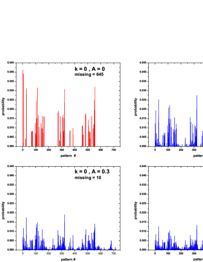
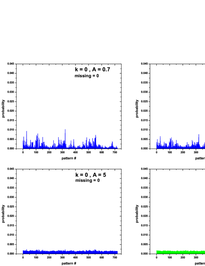
Figure 3: The Bandt-Pompe PDF ($M=720$) for a typical noisy chaotic time series considered (uncorrelated noise $k=0$), for different increasing values of the noise amplitude $A$. In the top-left corner the PDF corresponding to the unperturbed logistic map ($A=0$) is presented. In the bottom-right corner, the PDF for a pure noise $k=0$ time series is display. The values shown were obtained from times series of length $N=10^{5}$, and Bandt-Pompe parameters $D=6$, $\tau=1$.

Consider our results for uncorrelated noise $k=0$ and increasing values of noise-amplitude $A$ depicted in Fig. 2. This graph reveals that for $A\geq 1$ the points corresponding to increasing values of $A$ continue to move in the plane towards the site representative of pure noise, with ${\mathcal{M}}(N,D)=0$. The perturbative character of the noise is, of course, lost. This behavior is apparent in Fig. 3, where the corresponding Bandt-Pompe PDF’s, for a typical noisy chaotic time-series, are displayed for increasing noise amplitudes $A$. The corresponding value of ${\mathcal{M}}(N,D)$ can also be observed in these graphs.

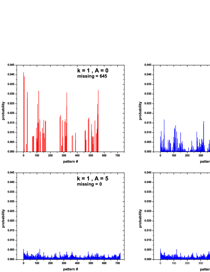
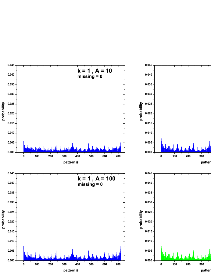
Figure 5: The Bandt-Pompe PDF ($M=720$) for a typical noisy chaotic time series considered (correlated noise $k=1$), for different increasing increasing values of the noise amplitude $A$. In the top-left corner the PDF corresponding to the unperturbed logistic map ($A=0$) is presented. In the bottom-right corner, the PDF for a pure noise $k=1$ time series is display. The values shown were obtained from times series of length $N=10^{5}$, and Bandt-Pompe parameters $D=6$, $\tau=1$.

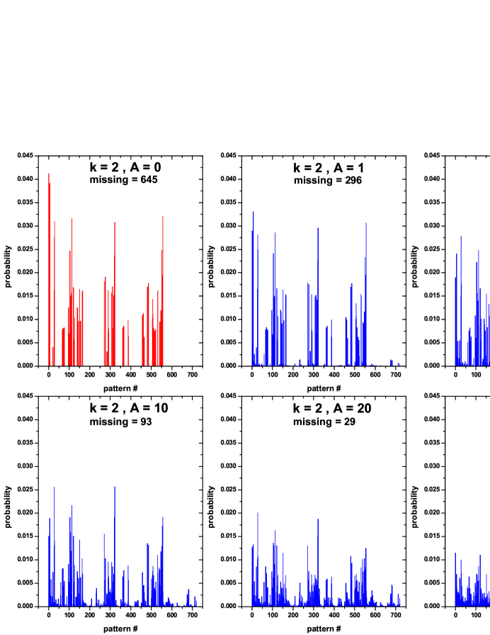
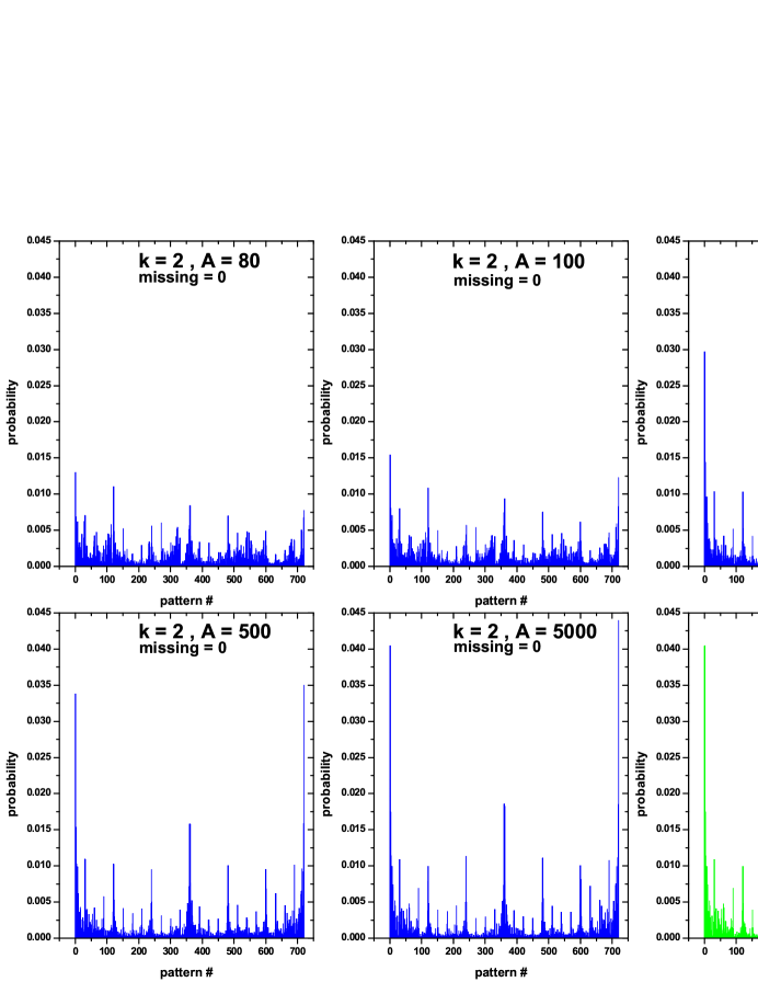
Figure 7: The Bandt-Pompe PDF ($M=720$) for a typical noisy chaotic time series considered (correlated noise $k=2$), for different increasing values of the noise amplitude $A$. In the top-left corner the PDF corresponding to the unperturbed logistic map ($A=0$) is presented. In the bottom-right corner, the PDF for a pure noise $k=2$ time series is display. The values shown were obtained from times series of length $N=10^{5}$, and Bandt-Pompe parameters $D=6$, $\tau=1$.

At the top-left corner of Fig. 3 we depict the Bandt-Pompe’s PDF for the unperturbed logistic map ($A=0$). The presence of forbidden patterns (that have probabilities $p_{i}=0$) is clearly visible. In the same plot, at the bottom-right corner, we display the pure noise $k=0$ (white noise) PDF. No forbidden patterns exist now, and we observe the characteristic flat distribution, $p_{i}\cong 1/M$ for all patterns $i=1,\cdots,M$ ($M=D!=720)$. The noise-influence on the PDFs is clearly displayed in this graph (see also the plots for $k=1$ and $k=2$, Figures 5 and 7). One appreciates the fact that the PDF evolves from that of the logistic map towards that of the pure-noise as one increases the value of $A$. The noise-effect also destroys the forbidden character of some patterns, whose associated probabilities grow slowly with the control parameter $A$, a feature that emphasizes the presence of a deterministic component in the noisy time series, even for ${\mathcal{M}}(N,D)=0$, if $A$ is not too large. This effect disappears for very strong noise. Note that for $A=5$ the PDF is practically equal to that of pure noise. The two PDFs are almost indistinguishable at $A=10$, and their planar localizations coincide (see Fig. 2).

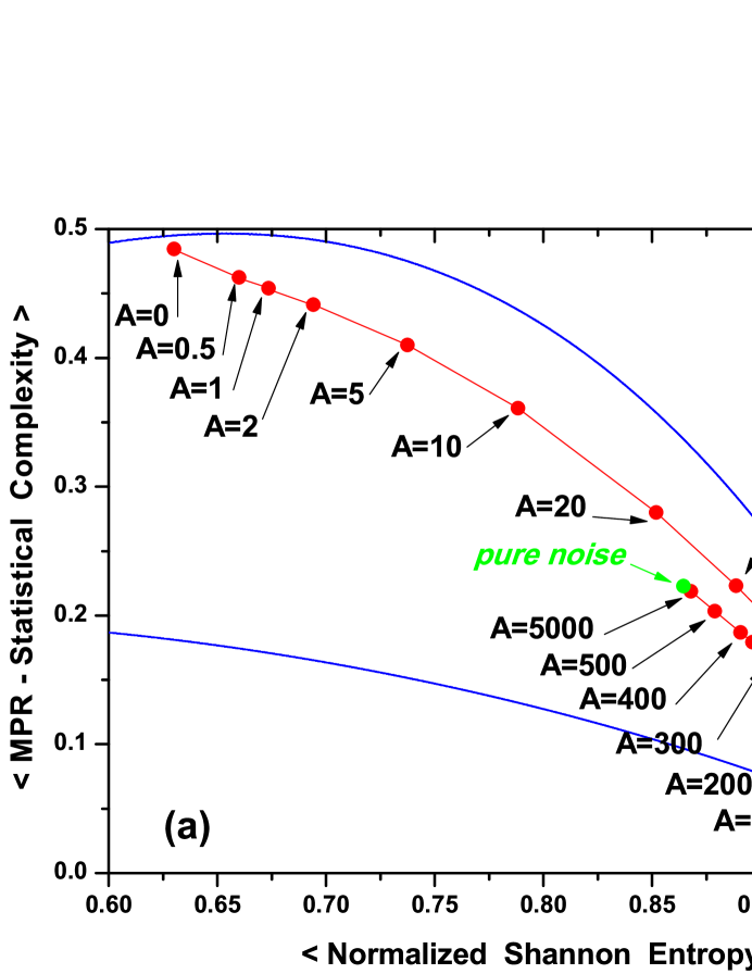
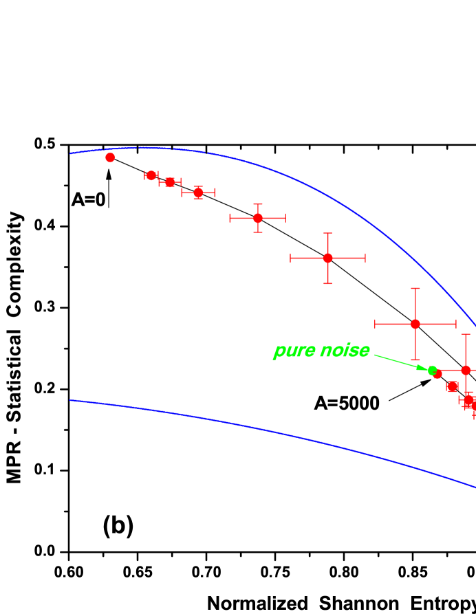
Figure 6: a) The causality entropy-complexity plane for all time series values (mean) corresponding to increasing values of noise amplitude $A$ and $k=2$. Value for the case of strictly noisy time series is shown as open symbol. The values shown were obtained from times series of length $N=10^{5}$, and Bandt-Pompe parameters $D=6$, $\tau=1$. The lines represent the values of minimum and maximum statistical complexity ${\mathcal{C}}_{min}$ and ${\mathcal{C}}_{max}$ evaluated for the case of pattern length $D=6$. b) Same, showing mean values and standard deviation for each $A$ considered value.

In Figures 4 and 6 one can appreciate details of the planar-localization of noisy chaotic time-series (mean values taken over ten realizations) that emerge out of the noise-contaminated logistic map. We display values for correlated noise with $k=1$ and $k=2$, with increasing noise amplitude $A\geq 1$. In these plots we also observe the planar locations of both the time-series for the unperturbed logistic map ($A=0$) and the pure-correlated noise ($k=1,2$). As in the previous case of uncorrelated noise ($k=0$), the planar locations move towards the pure-noise’s site (in the present cases, $k=1$ and $k=2$-pure noise, respectively) for increasing values of the noise-amplitude $A$. New behaviors emerge, as reflected by Figures 4 and 6. For varying noise-amplitude values we appreciate two different trajectories: 1) displacement on the associated planar locations from left to right (starting form the unperturbed value $A=0$), until reaching a point associated with a critical value $A_{c}$: $A_{c}\cong 7$ for $k=1$ (see Fig. 4) and $A_{c}\cong 80$ for $k=2$ (see Fig. 6). 2) At these critical values the trajectory reverses its direction (now it moves from right to left, “below” the first curve). The two trajectories converge at the planar location of the pure-correlated noise. Identical behavior was observed for all correlated noises with $k$-values in the interval $0<k<2$, that exhibit specific critical values of $A_{c}(k)$.

The planar behavior of the noisy, chaotic time-series can be interpreted in terms of two main interacting effects, namely, those associated with a) the persistence and robustness of the forbidden patterns in the deterministic chaotic component of the time-series and, b) the correlations characterizing stochastic observational noise (which in the present cases do not display forbidden patterns). These correlations grow with increasing values of $k>0$. Looking to the associated Bandt-Pompe’s PDFs behavior, depicted in Figs. 5 and 7 for different values of $A$, the observed planar trajectories can be succinctly described as itemized below.

• Amplitude range $0<A\leq A_{c}$: We deal with a two scenarios, one (Case A) in which the correlated noise acts as a perturbation ($\mathcal{M}(N,D)\neq 0$). In the other one (Case B) the logistic and the correlated noise have the same hierarchy ($\mathcal{M}(N,D)=0$). Fig. 6.b shows that for $k=2$ and case A the entropic and complexities’ dispersion (given by the standard deviation) are both small and due to the perturbative noise. Contrariwise, for case B the dispersion values increase with the noise amplitude $A$.

• Amplitude range $A\geq A_{c}$: Now the correlated noise dominates. The deterministic component of the time series can be considered here as a perturbation. Again, for this range of noise amplitudes we have ${\mathcal{M}}(N,D)=0$. We also observe that the dispersions of the entropy ${\mathcal{H}}_{s}$ and the complexity ${\mathcal{C}}_{JS}$ are small.

5 Conclusions

We have revisited in some detail the paradigmatic concept of forbidden/missing ordinal patterns and used it as a tool for distinguishing between deterministic and stochastic behavior in empiric time-series. In the spirit of [13, 14, 15, 18, 19, 20], we extended this kind of analysis by linking it to the physics described by the causality entropy-complexity plane [11]. Our considerations were made with regards to deterministic, finite time series contaminated with additive noises of different degree of correlation. Our analysis of the noise-determinism competition clearly demonstrates that forbidden patterns are a deterministic feature of nonlinear systems and also reaffirms the usefulness of the entropy-complexity plane as a powerful tool of the theoretical arsenal.

The planar localization in the causal entropy-complexity plane describing an uncontaminated, nonlinear deterministic system is displaced, by the addition of noise, towards a zone typical of pure stochasticity. This displacement generates a kind of trajectory in the ${\mathcal{H}}\times{\mathcal{C}}$-plane that is located in the vicinity of the curve corresponding to maximum statistical complexity.

If the noise is uncorrelated (white noise), the displacement of the system s characteristic point in the ${\mathcal{H}}\times{\mathcal{C}}$-plane becomes more pronounced as the noise intensity (amplitude) increases. It exhibits a monotonic decreasing behavior (from pure determinism to pure stochasticity). The noise-effect tends to eliminate forbidden patterns. Since these, in turn, are features of a deterministic dynamics, their destruction signals deterministic-nature’s loss.

For contaminating correlated noise a new type of planar trajectory-behavior emerges as the noise intensity increases. Starting from a pure deterministic localization, the trajectory converges to a pure stochastic localization by following a loop-curve as the noise intensity increases. For a critical value of noise intensity ($A_{c}$), however, this trajectory reverses direction. One observes a planar-movement of the system s characteristic point that starts at the unperturbed value ($A=0$) and closely approaches the curve of maximum complexity, from left to right, with increasing entropic values. At the critical noise intensity ($A_{c}$) this displacement reverses direction. It takes place now from right to left, below the original curve and converging to the planar location typical of pure-correlated noise. The value of the critical intensity $A_{c}$ depends on the correlation degree of the noise and on the deterministic component.

Three different scenarios can be associated:

1. The correlated noise acting as a perturbation and ${\mathcal{M}}(N,D)\neq 0$. The net noise effect is to destroy the forbidden character of some of the patterns. However due to the low noise intensity and to its correlations, the number of affected patterns is relatively low. The dominance of the deterministic component over the noisy one is reflected by low dispersion values for both the entropy and the statistical complexity.

2. The deterministic and the stochastic components have the same hierarchy and ${\mathcal{M}}(N,D)=0$. However, the persistent character of the forbidden patterns of the deterministic component and its interplay with the correlations present in the noise is reflected in the system s characteristic point trajectory, that moves along the curve of maximum complexity, indicating that the pertinent patterns do not appear as frequently as the remaining ones. This behavior is indicative of a still active deterministic dynamics. The dispersion values for our two quantifiers increase with the noise intensity.

The two scenarios above correspond to a noise intensity-range $0\leq A\leq A_{c}$.

1. The noisy component is the dominating one and the deterministic part can be considered as a perturbation. This scenario corresponds to the noise intensity range $A\geq A_{c}$ and we have ${\mathcal{M}}(N,D)=0$ as well, with low dispersion values for entropy and statistical complexity.

6 Appendix

6.1 MPR-Statistical Complexity

Given any arbitrary discrete probability distribution $P=\{p_{i}:i=1,\cdots,M\}$, with $M$ the number of freedom-degrees, Shannon’s logarithmic information measure reads [28]

$${\mathrm{S}}[P]=-\sum_{i=1}^{M}p_{i}\ln(p_{i})\ .$$ (3)

The Shannon entropy is a measure of the uncertainty associated to the physical process described by $P$. It is widely known that an entropic measure does not quantify the degree of structure or patterns present in a process [29]. Other measures of statistical or structural complexity, able capture their organizational properties, are necessary for a better understanding of chaotic time series [30]. Our group introduced an effective statistical complexity measure (SCM) that is able to detect essential details of the dynamics and differentiate different degrees of periodicity and chaos [31]. This specific SCM, abbreviated as the MPR-complexity one, provides important additional information regarding the peculiarities of the underlying probability distribution, not already detected by the entropy. It is defined, following the seminal, intuitive notion advanced by López-Ruiz et al. [32], via

$${\mathcal{C}}_{JS}[P]={\mathcal{Q}}_{J}[P,P_{e}]\cdot{\mathcal{H}}_{S}[P],$$ (4)

using:

• The normalized Shannon entropy ($0\leq{\mathcal{H}}_{S}\leq 1$)

  $${\mathcal{H}}_{S}[P]={\mathrm{S}}[P]/{\mathrm{S}}_{max}\ ,$$ (5)

  where ${\mathrm{S}}_{max}={\mathrm{S}}[P_{e}]=\ln M$ and $P_{e}=\{1/M,\cdots,1/M\}$ the uniform distribution.

• The so-called disequilibrium ${\mathcal{Q}}_{J}$ ($0\leq{\mathcal{Q}}_{J}\leq 1$), a quantifier defined in terms of the extensive (in the thermodynamical sense) Jensen-Shannon divergence ${\mathcal{J}}[P,P_{e}]$ that links two PDFs. We have

  $${\mathcal{Q}}_{J}[P,P_{e}]=Q_{0}\cdot{\mathcal{J}}[P,P_{e}]\ ,$$ (6)

  with

  $${\mathcal{J}}[P,P_{e}]={\mathrm{S}}\left[(P+P_{e})/2\right]-{\mathrm{S}}[P]/2-{\mathrm{S}}[P_{e}]/2\ .$$ (7)

  $Q_{0}$ is a normalization constant, equal to the inverse of the maximum possible value of ${\mathcal{J}}[P,P_{e}]$. This value is obtained when one of the values of $P$, say $p_{m}$, is equal to one and the remaining $p_{i}$ values are equal to zero, i.e.,

  $$Q_{0}~{}=~{}-2\left\{\left(\frac{M+1}{M}\right)\ln(M+1)-2\ln(2M)+\ln M\right\}^{-1}\ .$$ (8)

The Jensen-Shannon divergence, that quantifies the difference between two (or more) probability distributions, is especially useful to compare the symbol-composition of different sequences [33]. The complexity measure constructed in this way has the intensive property found in many thermodynamic quantities [31]. We stress the fact that the statistical complexity defined above is the product of two normalized entropies (the Shannon entropy and Jensen-Shannon divergence), but it is a nontrivial function of the entropy because it depends on two different probabilities distributions, i.e., the one corresponding to the state of the system, $P$, and the uniform distribution, $P_{e}$.

6.2 Entropy-Complexity plane

The time-evolution of the MPR-complexity can be analyzed using a diagram of ${\mathcal{C}}_{JS}$ versus time $t$. Thermodynamics’ second law states that for isolated systems the entropy grows monotonically with time ($d{\mathcal{H}}_{S}/dt\geq 0$), entailing that ${\mathcal{H}}_{S}$ can be viewed an “arrow of time” [34]. This suggests to study the temporal evolution of the SCM via an analysis of ${\mathcal{C}}_{JS}$ versus ${\mathcal{H}}_{S}$. A normalized entropy-axis substitutes for the time-axis. Since one knows that for a given value of ${\mathcal{H}}_{S}$ the range of possible MPR-complexity values varies between a minimum ${\mathcal{C}}_{min}$ and a maximum ${\mathcal{C}}_{max}$ [35], our evolutionary path must take place in the planar-region delimited by these curves. It was demonstrated that evolutionary path analysis generates insight into the details of the system s probability distribution (not provided by randomness measures like the entropy [11, 30]) that helps to uncover information related to the correlational structure between the components of a given physical process [36, 37].

6.3 Estimation of the Probability Distribution Function

Before attempting the time series characterization using Information Theory quantifiers, a probability distribution function (PDF) associated to the time series under analysis should be provided beforehand. The determination of the most adequate PDF is a fundamental problem because $P$ and the sample space $\Omega$ are inextricably linked. Many methods have been proposed for a proper selection of the probability space $(\Omega,P)$. We can mention: (a) frequency counting [38], (b) procedures based on amplitude statistics [39], (c) binary symbolic dynamics [40], (d) Fourier analysis [41] and, (e) wavelet transform [42], among others. Their applicability depends on particular characteristics of the data, such as stationarity, time series length, variation of the parameters, level of noise contamination, etc. In all these cases the dynamics’ global aspects can be somehow captured, but the different approaches are not equivalent in their ability to discern all the relevant physical details. One must also acknowledge the fact that the above techniques are introduced in a rather “ad hoc fashion” and they are not directly derived from the dynamical properties themselves of the system under study.

A better procedure is provided by the symbolic analysis of the time series, that discretizes the raw series and transforms it into a sequence of symbols. Symbolic analysis is efficient for nonlinear data processing, with low sensitivity to noise [43]. Of course, meaningful symbolic representations of the original series are not provided by God and require some effort [44, 45]. Today many people are confident that the Bandt and Pompe approach for generating PDF’s is one of the most simple symbolization techniques and takes into account time-causality in the evaluation of the PDF associated to a time series [12]. Symbolic data are i) created by associating a rank to the series-values and ii) defined by reordering the embedded data in ascending order. Data are reconstructed with an embedding dimension $D$. In this way it is possible to quantify the diversity of the ordering symbols (patterns) derived from a time series, evaluating the so called “permutation entropy” ${\mathcal{H}}_{S}$, and permutation statistical complexity ${\mathcal{C}}_{JS}$ (i.e., the normalized Shannon entropy and MPR-statistical complexity measure evaluated for the Bandt and Pompe’s PDF).

6.4 The Bandt and Pompe approach for PDF construction

Bandt and Pompe [12] introduced a simple and robust method to evaluate the probability distribution taking into account the time causality of the system dynamics. They suggested that the symbol sequence should arise naturally from the time series, without any model-based assumptions. Thus, they took partitions by comparing the order of neighboring values rather than partitioning the amplitude into different levels. That is, given a time series ${\mathcal{S}}=\{x_{t};t=1,\cdots,N\}$, an embedding dimension $D>1~{}(D\in{\mathbb{N}})$, and an embedding time delay $\tau$ ($\tau\in{\mathbb{N}}$), the ordinal pattern of order $D$ generated by

$$s\mapsto\left(x_{s-(D-1)\tau},x_{s-(D-2)\tau},\cdots,x_{s-\tau},x_{s}\right)\ ,$$ (9)

is to be considered. To each time $s$ we assign a $D$-dimensional vector that results from the evaluation of the time series at times $s-(D-1)\tau,\cdots,s-\tau,s$. Clearly, the higher the value of $D$, the more information about the past is incorporated into the ensuing vectors. By the ordinal pattern of order $D$ related to the time $s$ we mean the permutation $\pi=(r_{0},r_{1},\cdots,r_{D-1})$ of $(0,1,\cdots,D-1)$ defined by

$$x_{s-r_{D-1}\tau}\leq x_{s-r_{D-2}\tau}\leq\cdots\leq x_{s-r_{1}\tau}\leq x_{s-r_{0}\tau}\ .$$ (10)

In this way the vector defined by Eq. (9) is converted into a unique symbol $\pi$. In order to get a unique result we consider that $r_{i}<r_{i-1}$ if $x_{s-r_{i}\tau}=x_{s-r_{i-1}\tau}$. This is justified if the values of ${x_{t}}$ have a continuous distribution so that equal values are very unusual.

For all the $D!$ possible orderings (permutations) $\pi_{i}$ when the embedding dimension is $D$, their associated relative frequencies can be naturally computed by the number of times this particular order sequence is found in the time series divided by the total number of sequences,

$$p(\pi_{i})~{}=~{}\frac{\sharp\{s|s\leq N-(D-1)\tau;(s)\quad\texttt{has type}~{}\pi_{i}\}}{N-(D-1)\tau}\ .$$ (11)

In the last expression the symbol $\sharp$ stands for “number”. Thus, an ordinal pattern probability distribution $P=\{p(\pi_{i}),i=1,\cdots,D!\}$ is obtained from the time series.

It is clear that this ordinal time-series’ analysis entails losing some details of the original amplitude-information. Nevertheless, a meaningful reduction of the complex systems to their basic intrinsic structure is provided. Symbolizing time series, on the basis of a comparison of consecutive points allows for an accurate empirical reconstruction of the underlying phase-space of chaotic time-series affected by weak (observational and dynamical) noise [12]. Furthermore, the ordinal-pattern probability distribution is invariant with respect to nonlinear monotonous transformations. Thus, nonlinear drifts or scalings artificially introduced by a measurement device do not modify the quantifiers’ estimations, a relevant property for the analysis of experimental data. These advantages make the BP approach more convenient than conventional methods based on range partitioning. Additional advantages of the Bandt and Pompe method reside in its simplicity (we need few parameters: the pattern length/embedding dimension $D$ and the embedding time lag $\tau$) and the extremely fast nature of the pertinent calculation-process [46, 47]. We stress that the Bandt and Pompe’s methodology is not restricted to time series representative of low dimensional dynamical systems but can be applied to any type of time series (regular, chaotic, noisy, or reality based), with a very weak stationary assumption (for $k=D$, the probability for $x_{t}<x_{t+k}$ should not depend on $t$ [12]).

The probability distribution $P$ is obtained once we fix the embedding dimension $D$ and the embedding time delay $\tau$. The former parameter plays an important role for the evaluation of the appropriate probability distribution, since $D$ determines the number of accessible states, given by $D!$. Moreover, it has been established that the length $N$ of the time series must satisfy the condition $N\gg D!$ in order to achieve a proper differentiation between stochastic and deterministic dynamics [11]. With respect to the selection of the parameters, Bandt and Pompe suggest in their cornerstone paper [12] to work with $3\leq D\leq 7$ with a time lag $\tau=1$. Nevertheless, other values of $\tau$ might provide additional information. Soriano et al. [48, 49] and Zunino et al. [50] recently showed that this parameter is strongly related, when it is relevant, with the intrinsic time scales of the system under analysis. In the present work $D=6$ and $\tau=1$ are used. Of course it is also assumed that enough data are available for a correct embedding-time delay procedure (attractor-reconstruction).

References

- [1] A. R. Osborne, A. Provenzale, Finite correlation dimension for stochastic systems with power-law spectra. Physica D 35 (1989) 357–381.
- [2] G. Sugihara, R. M. May, Nonlinear forecasting as a way of distinguishing chaos from measurement error in time series. Nature 344 (1983) 734–741.
- [3] D. T. Kaplan, L. Glass, Direct test for determinism in a time series. Phys. Rev. Lett. 68 (1992) 427–430.
- [4] D. T. Kaplan, L. Glass, Coarse-grained embeddings of time series: random walks, Gaussian random processes, and deterministic chaos. Physica D 64 (1993) 431–454.
- [5] H. Kantz, E. Olbrich, Coarse grained dynamical entropies: Investigation of high-entropic dynamical systems. Physica A 280 (2000) 34–48.
- [6] M. Cencini, M. Falcioni, E. Olbrich, H. Kantz, A. Vulpiani, Chaos or noise: Difficulties of a distinction. Physica A 280 (2000) 34–48.
- [7] H. Kantz, T. Scheiber, Nonlinear Time Series Analysis. Cambridge University Press, Cambridge, UK, 2002.
- [8] H. D. I. Abarbanel, Analysis of Observed Chaotic Data. Springer-Verlag, New York, USA, 1996.
- [9] A. N. Kolmogorov, A new metric invariant for transitive dynamical systems and automorphisms in lebesgue sapces. Dokl. Akad. Nauk., USSR , 119 (1959) 861 – 864.
- [10] Y. G. Sinai, On the concept of entropy for a dynamical system. Dokl. Akad. Nauk., USSR , 124 (1959) 768 – 771.
- [11] O. A. Rosso, H. A Larrondo, M. T. Martín, A. Plastino, M. A. Fuentes, Distinguishing noise from chaos. Phys. Rev. Lett. 99 (2007) 154102.
- [12] C. Bandt, B. Pompe, Permutation entropy: a natural complexity measure for time series. Phys. Rev. Lett. 88 (2002) 174102.
- [13] J. M. Amigó, L. Kocarev, J. Szczepanski, Order patterns and chaos Phys. Lett. A 355 (2006) 27 -31.
- [14] J. M. Amigó, S. Zambrano, M. A. F. Sanjuán, True and false forbidden patterns in deterministic and random dynamics. Europhys. Lett. 79 (2007) 50001.
- [15] J. M. Amigó, S. Zambrano and M. A. F. Sanjuán, Combinatorial detection of determinism in noisy time series. Europhys. Lett. 83 (2008) 60005.
- [16] J. M. Amigó, Permutation complexity in dynamical systems. Springer-Verlag, Berlin, Germany, 2010.
- [17] L. C. Carpi, P. M. Saco, O. A. Rosso, Missing Ordinal Patterns in Correlated Noises. Physica A 389 (2010) 2020–2029.
- [18] M. Zanin, Forbidden patterns in financial time series. Chaos 18 (2008) 013119.
- [19] L. Zunino, M. Zanin, B. M. Tabak, D. Pérez, O. A. Rosso, Forbidden patterns, permutation entropy and stock market inefficiency. Physica A 388 (2009) 2854 – 2864.
- [20] G. Ouyang, X. Li, C. Dang and D. A. Richards, Deterministic dynamics of neural activity during absence seizures in rats. Phys. Rev. E 79 (2009) 041146.
- [21] O.A. Rosso, L. C. Carpi, M. P. Saco, M. Gómez Ravetti, A. Plastino, H. A. Larrondo. Causality and the entropy-complexity plane: robustness and missing ordinal patters. Physica A (2011) in press, DOI: 10.1016/j.physa.2011.07.030
- [22] O. A. Rosso, L. De Micco, H. Larrondo, M. T. Martín, A. Plastino. Generalized statistical complexity measure. Int. J. Bif. and Chaos 20 (2010) 775–785.
- [23] J. C. Sprott, Chaos and Time Series Analysis, Oxford University Press, Oxford, 2004.
- [24] M. Matsumoto, T. Nishimura, Mersenne twister: a 623-dimensionally uniform pseudo-random number generator. ACM Transactions on Modeling and Computer Simulation 8 (1998) 3 – 30.
- [25] H. Wold, A Study in the Analysis of Stationary Time Series. Almqvist and Wiksell, Upsala, Sweden, 1938.
- [26] J. Kurths, H. Herzel, An attractor in a solar time series. Physica D 25 (1987) 165 – 172.
- [27] S. Cambanis, C. D. Hardin, A. Weron, Innovations and Wold decompositions of stable sequences. Probab. Theory Relat. Fields 79 (1988) 1 – 27.
- [28] C. Shannon, W. Weaver, The Mathematical Theory of Communication University of Illinois Press, Champaign, IL, 1949.
- [29] D. P. Feldman, J. P. Crutchfield, Measures of statistical complexity: Why?. Phys. Lett. A 238 (1998) 244 – 252.
- [30] D. P. Feldman, C. S. McTague, J. P. Crutchfield, The organization of intrinsic computation: Complexity-entropy diagrams and the diversity of natural information processing. Chaos 18 (2008) 043106.
- [31] P. W. Lamberti, M. T. Martín, A. Plastino, and O. A. Rosso, Intensive entropic nontriviality measure. Physica A 334 (2004) 119 – 131.
- [32] R. López-Ruiz, H. L. Mancini, X. Calbet, A statistical measure of complexity. Phys. Lett. A 209 (1995) 321 – 326.
- [33] I. Grosse, P. Bernaola-Galván, P. Carpena, R. Román-Roldán, J. Oliver, H. E. Stanley, Analysis of symbolic sequences using the Jensen-Shannon divergence. Phys. Rev. E 65 (2002) 041905.
- [34] A. R. Plastino, and A. Plastino, Symmetries of the Forker-Plank equation and Fisher-Frieden arrow of time. Phys. Rev. E 54 (1996) 4423 – 4326.
- [35] M. T. Martín, A. Plastino, O. A. Rosso, Generalized statistical complexity measures: geometrical and analytical properties. Physica A 369, 439 (2006) 439 – 462.
- [36] O. A. Rosso, C. Masoller. Detecting and quantifying stochastic and coherence resonances via Information Theory complexity measurements. Phys. Rev. E 79 (2009) 040106(R).
- [37] O. A. Rosso, C. Masoller. Detecting and quantifying temporal correlations in stochastic resonance via Information Theory measures. European Phys. Journal B, 69 (2009) 37–43.
- [38] O. A. Rosso, H. Craig, P. Moscato, Shakespeare and other English renaissance authors as characterized by Information Theory complexity quantifiers. Physica A 388 (2009) 916 – 926
- [39] L. De Micco, C. M. González, H. A. Larrondo, M. T. Martín, A. Plastino, O. A. Rosso, Randomizing nonlinear maps via symbolic dynamics. Physica A 87 (2008) 3373 - 3383.
- [40] K. Mischaikow, M. Mrozek, J. Reiss, A. Szymczak, Construction of symbolic dynamics from experimental time series. Phys. Rev. Lett. 82 (1999) 1114 - 1147.
- [41] G. E. Powell, I. C. Percival, A spectral entropy method for distinguishing regular and irregular motion of hamiltonian systems. J. Phys. A: Math. Gen. 12 (1979) 2053 - 2071.
- [42] O. A. Rosso, S. Blanco, J. Jordanova, V. Kolev, A. Figliola, M. Schürmann, E. Başar, Wavelet entropy: a new tool for analysis of short duration brain electrical signals. J. Neurosc. Meth. 105 (2001) 65 -75.
- [43] J. M. Finn, J. D. Goettee, Z. Toroczkai, M. Anghel, B. P. Wood, Estimation of entropies and dimensions by nonlinear symbolic time series analysis. Chaos 13, 444 (2003) 444 – 457.
- [44] E. M. Bollt, T. Stanford, Y. C. Lai, K. Życzkowski, Validity of Threshold-Crossing Analysis of Symbolic Dynamics from Chaotic Time Series. Phys. Rev. Lett. 85 (2000) 3524 – 3527.
- [45] C. S. Daw, C. E. A. Finney, E. R. Tracy, A review of symbolic analysis of experimental data. Rev. Sci. Instrum. 74 (2003) 915 – 931.
- [46] K. Keller, M. Sinn. Ordinal analysis of time series. Physica A 356 (2005) 114–120.
- [47] K. Keller, H. Lauffer. Symbolic analysis of high-dimensional time series. Int. J. Bifurcation and Chaos 13 (2003) 2657–2668.
- [48] M. C. Soriano, L. Zunino, L. Larger, I. Fischer, and C. R. Mirasso ). opto-electronic oscillator. Optics Letters 36 (2010) 2212–2214.
- [49] M. C. Soriano, M. C., L. Zunino, O. A. Rosso, I. Fischer, C. R. Mirasso. Time scales of a chaotic semiconductor laser with optical feedback under the lens of a permutation information analysis. IEEE J. Quantum Electron. 47 (2010) 252–261.
- [50] L. Zunino, M. C. Soriano, I. Fischer, O. A. Rosso, C. R. Mirasso. Permutation information theory approach to unveil delay dynamics from time series analysis. Phys. Rev. E 82 (2010) 046212.