Radiation interference from sources rotating around Schwarzschild black holes

Abstract

We investigate the influence of the spacetime curvature on the interference of the radiation emitted by an ensemble of scalar sources in circular motion around a Schwarzschild black hole. We pay particular attention to the transition from the radiating to the non-radiating regime as the number of sources increases.

I Introduction

Astrophysical evidences for the presence of black holes in certain X-ray binary systems as well as in the center of many galaxies are mounting Astro . The fact that many observational data on black holes come from photons emitted by surrounding matter has motivated a more detailed investigation of radiation processes in these non-trivial backgrounds. In the early seventies, Misner and collaborators championed a research program focusing on the synchrotron radiation emitted by fast moving charges orbiting black holes Misneretal ; Breuer . Since then, related studies have been pursued in various situations of interest in both classical and quantum frameworks (see, e.g., Refs. P95 -CdM09 and references therein). In all these papers, however, attention was restricted to the radiation emitted by individual sources. As we are often interested in physical situations where a large number of charges are present (e.g., in accretion disks of compact objects), a more comprehensive analysis considering the combined emission of various sources would be welcome. In this paper, we investigate the scalar radiation emitted by an ensemble of sources in geodesic orbits around a Schwarzschild black hole. We focus on the effect of the spacetime curvature on the radiation interference and pay particular attention to the transition from the radiating to the non-radiating (“magnetostatic”) regime as the number of sources increases.

The paper is organized as follows. In section II, we present the quantum field theory framework in which we work and establish the general formulas which will be used further to calculate the observables of interest. In section III, we apply the previous section results to investigate the scalar radiation emitted by certain source configurations and discuss the corresponding interference effects. Section IV is dedicated to our final remarks. We assume natural units $c=\hbar=G=1$ (unless stated otherwise) and metric signature $(+---)$.

II General Framework

The spherically symmetric vacuum solution of Einstein equations describing a black hole with mass $M$ is

$$ds^{2}=f(r)dt^{2}-f(r)^{-1}dr^{2}-r^{2}(d\theta^{2}+\sin^{2}\theta d\varphi^{2}),$$ (1)

where $f(r)=1-2M/r$. Now, we introduce $N$ point scalar sources in uniform circular motion composing a thin disk at the equatorial plane, $\theta=\pi/2$, with four-velocities

$$u_{i}^{\mu}(\Omega_{i},R_{i})=(f(R_{i})-R_{i}^{2}\Omega_{i}^{2})^{-1/2}(1,0,0,\Omega_{i}),$$ (2)

where $i=1,\ldots,N$ labels the sources, $R_{i}$ denotes the radial coordinates, and $\Omega_{i}$ stands for the constant angular velocities as defined by asymptotic static observers. The corresponding total source density is given by

$$j(x^{\nu})=\sum_{i=1}^{N}j_{i}(x^{\nu}),$$

where

$$j_{i}(x^{\nu})={\frac{q_{i}}{\sqrt{-g}\,u_{i}^{0}}\delta(r-R_{i})\delta(\theta-\pi/2)\delta(\varphi-\Omega_{i}t-\lambda_{i})}$$ (3)

is normalized so that

$$\int{d\sigma_{i}j_{i}(x^{\nu})}=q_{i}$$

and $d\sigma_{i}$ is the proper 3-volume element orthogonal to $u^{\mu}_{i}$. Here $g\equiv\det(g_{\mu\nu})$ and $\lambda_{i}={\rm const}$ defines the initial angular positions.

We minimally couple $j(x^{\mu})$ to a real massless scalar field $\hat{\Phi}$ according to the interaction Lagrangian density

$$\mathcal{L}=\sqrt{-g}j(x^{\nu})\hat{\Phi}.$$ (4)

The free scalar field operator $\hat{\Phi}$ satisfies the massless Klein-Gordon equation $\Box\hat{\Phi}=0$ and can be expanded in terms of creation $a^{\dagger}_{\alpha\omega lm}$ and annihilation $a_{\alpha\omega lm}$ operators as

$$\hat{\Phi}=\sum_{\alpha=\rightarrow}^{\leftarrow}\sum_{l=0}^{\infty}\sum_{m=-l}^{l}\int_{0}^{\infty}d\omega[u_{\alpha\omega lm}(x^{\mu})a_{\alpha\omega lm}+{\rm H.c.}],$$ (5)

where

$$[a_{\alpha\omega lm},a^{\dagger}_{\alpha^{\prime}\omega^{\prime}l^{\prime}m^{\prime}}]=\delta(\omega-\omega^{\prime})\delta_{ll^{\prime}}\delta_{mm^{\prime}}\delta_{\alpha\alpha^{\prime}}.$$

Here $\omega\geq 0$ denotes the scalar particle frequency, $l\geq 0$ is the azimuthal angular momentum quantum number, $m\in[-l,l]$, $\alpha$ labels outgoing modes ($\alpha=\rightarrow$) from the past white hole horizon ${\cal H}^{-}$ and incoming ones ($\alpha=\leftarrow$) from the past null infinity ${\cal J}^{-}$. The positive-frequency orthonormal solutions (with respect to the Klein-Gordon inner product birrel ) satisfying $\Box u_{\alpha\omega lm}=0$ are denoted by

$$u_{\alpha\omega lm}=\sqrt{\frac{\omega}{\pi}}\frac{\psi^{\alpha}_{\omega l}(r)}{r}Y_{lm}(\theta,\varphi)e^{-i\omega t},$$ (6)

where $Y_{lm}(\theta,\varphi)$ are the usual spherical harmonic functions and $\psi^{\alpha}_{\omega l}$ satisfy the differential equation

$$\left[-f(r)\frac{d}{dr}\left(f(r)\frac{d}{dr}\right)+V_{\rm S}(r)\right]\psi^{\alpha}_{\omega l}(r)=\omega^{2}\psi^{\alpha}_{\omega l}(r)$$ (7)

with

$$V_{\rm S}(r)\equiv(1-2M/r)[2M/r^{3}+l(l+1)/r^{2}].$$ (8)

For the sake of further convenience, it is useful to note that the scattering potential $V_{\rm M}(r)$ associated with Minkowski spacetime can be obtained from $V_{\rm S}(r)$ by vanishing the black hole mass $M$ in Eq. (8): $V_{\rm S}(r)\stackrel{{\scriptstyle M\to 0}}{{\longrightarrow}}V_{\rm M}(r)\equiv l(l+1)/r^{2}$. In contrast to the Schwarzschild case where $\psi^{\alpha}_{\omega l}$ can be expressed in terms of simple functions only in the low- and high-frequency regimes, the (single) set of normalizable radial functions in the Minkowski case can be written in terms of usual spherical Bessel functions as $\psi^{M}_{\omega l}(r)=rj_{l}(\omega r)$ for all $\omega$.

In the low-frequency regime, the leading terms of the radial functions in the Schwarzschild case are (up to an arbitrary phase) HMC1998

$$\psi^{\rightarrow}_{\omega l}(r)\approx 2rQ_{l}(r/M-1)$$ (9)

and

$$\psi^{\leftarrow}_{\omega l}(r)\approx\frac{2^{2l}(l!)^{3}(M\omega)^{l}rP_{l}(r/M-1)}{(2l)!(2l+1)!},$$ (10)

where $P_{l}(x)$ and $Q_{l}(x)$ are Legendre functions. In the high-frequency regime, good results can be obtained using the WKB method CdM09 :

$$\psi^{\rightarrow}_{\omega l}(x)\approx-i\sqrt{\frac{M}{2\omega\kappa_{\omega l}}}e^{\xi_{\omega l}(x)-\Theta_{\omega l}},$$ (11)

$$\psi^{\leftarrow}_{\omega l}(x)\approx-i\sqrt{\frac{M}{2\omega\kappa_{\omega l}}}e^{-\xi_{\omega l}(x)},$$ (12)

where $x\equiv r/2M+\ln(r/2M-1)$ is the dimensionless tortoise radial coordinate and $\kappa_{\omega l}\equiv 2M\sqrt{V_{\rm S}(x)-\omega^{2}}\equiv ik_{\omega l}$. Here, we have defined

$$\xi_{\omega l}(x)\equiv\int_{x}^{x_{+}}{\kappa_{\omega l}(x^{\prime})dx^{\prime}}$$ (13)

and the barrier factor

$$\Theta_{\omega l}\equiv\int_{x_{-}}^{x_{+}}{\kappa_{\omega l}(x)dx},$$ (14)

where $x_{-}$ and $x_{+}$ stand for the classical turning points satisfying $V_{S}(x_{\pm})=\omega^{2}$. The WKB method guaranties good results as long as $k_{\omega l}^{-1}d(\ln k_{\omega l})/dx\ll 1$ but it is worthwhile to keep in mind that full numerical calculations show that this approximation satisfactorily captures the qualitative behavior of the radial functions in the low-frequency sector besides leading to excellent results in the high-frequency regime CdM09 .

Our main observable of interest will be the emitted total power

$$W^{(N)}=\sum_{\alpha=\rightarrow}^{\leftarrow}\sum_{l=1}^{\infty}\sum_{m=1}^{l}W^{(N)}_{\alpha lm},$$ (15)

where

$$W^{(N)}_{\alpha lm}=\int_{0}^{\infty}d\omega\,\omega|{\cal A}_{\alpha\omega lm}|^{2}/T,$$ (16)

$T=2\pi\delta(0)$ is the total time as measured by asymptotic observers IZ , and

$${\cal A}_{\alpha\omega lm} = \langle\alpha\,\omega\,l\,m\,|i\int{d^{4}x\sqrt{-g}j(x^{\mu})\hat{\Phi}(x^{\mu})}|0\rangle$$ (17)

$$= i\int{d^{4}x\sqrt{-g\,}j(x^{\mu})u^{*}_{\alpha\omega lm}(x^{\mu})}$$

is the emission amplitude at the tree level associated with the emission of a scalar particle with quantum numbers $(\alpha,\omega,l,m)$ into the Boulware vacuum. We note that sources with $\Omega_{i}={\rm const}$ give rise to terms proportional to $\delta(\omega-m\Omega_{i})$ in the amplitude ${\cal A}_{\alpha\omega lm}$. Thus, $W^{(N)}$ will have no contributions coming from $m\leq 0$ if we assume that $\Omega_{i}>0$. This is already codified in Eq. (15).

III Radiation emission and interference

We now apply the formalism above to analyze the radiation emission from an ensemble of point sources in geodesic circular motion around a Schwarzschild black hole. In this case, the corresponding angular velocities $\Omega_{i}$ are related with the radial coordinates $R_{i}$ by

$$\Omega_{i}=(M/R_{i}^{3})^{1/2}.$$ (18)

It is particularly illuminating to investigate first the radiation interference restricting the number of sources to two, while allowing for an arbitrary angular separation between them. Afterwards, we consider a system of $N$ sources equally spaced around an orbit, which will be suited to our discussion about the transition from the radiating to the non-radiating regime. We shall compare the results obtained in Schwarzschild and Minkowski spacetimes in order to extract the very influence of the spacetime curvature in the interference phenomenon.

III.1 Two scalar sources

Let us introduce a two-scalar source system by writing $j(x^{\mu})=j_{1}(x^{\mu})+j_{2}(x^{\mu})$, where $j_{i}$ ($i=1,2$) is given by Eq. (3). We define $q_{1}\equiv q$ and $q_{2}=\pm q$, where the choice between $``+"$ and $``-"$ will simulate “charged” and “neutral” configurations, respectively. By fixing $\lambda_{1}=0$ and $\lambda_{2}\equiv\lambda$, we have

$$j(x^{\mu}) =\frac{q}{\sqrt{-g\,}u_{1}^{0}}\delta(r-R_{1})\delta(\theta-\pi/2)\delta(\varphi-\Omega_{1}t)$$

$$\pm\frac{q}{\sqrt{-g\,}u_{2}^{0}}\delta(r-R_{2})\delta(\theta-\pi/2)\delta(\varphi-\Omega_{2}t-\lambda).$$ (19)

The emitted power $W^{(2)}_{\alpha lm}$, as given by Eq. (16), can be cast as

$$W^{(2)}_{\alpha lm}=\sum_{i=1,2}{{}^{i}}W^{(1)}_{\alpha lm}+\,^{\rm int}\!W^{(2)}_{\alpha lm},$$ (20)

where

$${{}^{i}}W^{(1)}_{\alpha lm} = 2q^{2}m^{2}\Omega_{i}^{2}[f(R_{i})-R_{i}^{2}\Omega_{i}^{2}]|\psi^{\alpha}_{m\Omega_{i}\;l}(R_{i})/R_{i}|^{2}$$ (21)

$$\times |Y_{lm}(\pi/2,0)|^{2}$$

is the power emitted by each source $i=1,2$ separately and

$${}^{\rm int}W^{(2)}_{\alpha lm} = \pm\frac{8\pi q^{2}}{R_{1}R_{2}}\sqrt{f(R_{1})-R_{1}^{2}\Omega_{1}^{2}}\sqrt{f(R_{2})-R_{2}^{2}\Omega_{2}^{2}}$$ (22)

$$\times \psi^{\alpha}_{m\Omega_{1}\,l}(R_{1})\psi^{\alpha}_{m\Omega_{2}\,l}(R_{2})|Y_{lm}(\pi/2,0)|^{2}$$

$$\times m^{2}\cos(m\lambda)\Omega_{1}\Omega_{2}\,\delta(m\Omega_{2}-m\Omega_{1})/T$$

is the interference term associated with the two-scalar source system. The $\delta(m\Omega_{2}-m\Omega_{1})$ term implies that interference effects will only appear when $\Omega\equiv\Omega_{1}=\Omega_{2}$. (This is so because in this case there is a well-defined phase relationship between the emitted waves.) Hence, for sources in geodesic motion belonging to a thin disk, the interference term (22) will only contribute when the sources share the same orbit: $R\equiv R_{1}=R_{2}$ [see Eq. (18)]. We restrict our attention to this case, since the one where the sources do not share the same orbit does not offer a major challenge (once contributions coming from each source are summed up incoherently in the total power).

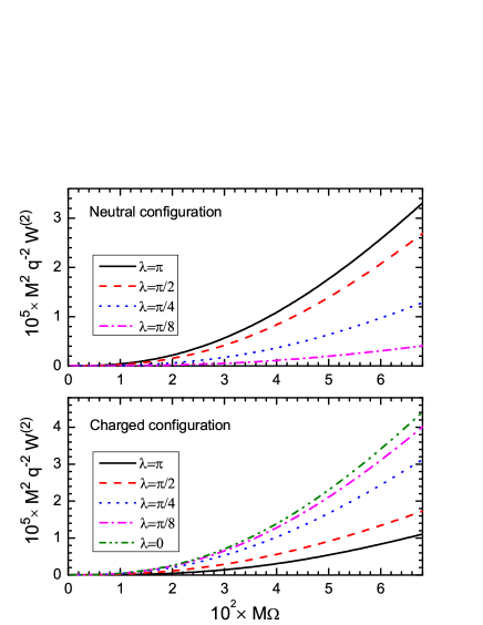
Figure 1: The total emitted power $W^{(2)}$ is plotted for stable circular geodesics, i.e. $M\Omega\leq 0.068$ ($R\geq 6M$), assuming various angular separations $\lambda$. Here, the low-frequency approximations (9)-(10) were used for the radial functions.

The total power (15) associated with a two-scalar source system where the sources at $r=R$ have angular velocities $\Omega$ and are separated by an angle $\lambda$ can be calculated using Eq. (20):

$$W^{(2)}=\sum_{\alpha=\rightarrow}^{\leftarrow}\sum_{l=1}^{\infty}\sum_{m=1}^{l}4q^{2}m^{2}\Omega^{2}(f(R)-R^{2}\Omega^{2})$$

$$\times\left|\frac{\psi^{\alpha}_{m\Omega\;l}(R)}{R}\right|^{2}|Y_{lm}(\pi/2,0)|^{2}[1\pm\cos(m\lambda)].$$ (23)

In Fig. 1, we plot the total emitted power $W^{(2)}$ as a function of $\Omega$ for several angular separations $\lambda$. For the sake of visual clarity, we only consider sources at stable circular geodesics, $R\geq 6M$. (For $3M<R<6M$ the same monotonic increase is observed.) We see that for the neutral configuration, the power is the largest for $\lambda=\pi$ (largest dipole moment) and goes to zero as $\lambda$ decreases. In the $\lambda\to 0$ limit, superposed sources, no radiation is emitted, as expected. On the other hand, for the charged configuration, the emitted power is maximum for $\lambda=0$ and minimum for $\lambda=\pi$, in which case $W^{(2)}_{\alpha 11}=0$ and the dominant multipole contribution comes from $l=2$. In order to plot Fig. 1, we have used the low-frequency approximation given by Eqs. (9)-(10) for $\psi^{\alpha}_{\omega l}$, since particles radiated away by sources at $R\geq 6M$ will typically possess frequencies $\omega$ satisfying

$$\omega/M^{-1}=m\Omega_{i}/M^{-1}<6.8\times 10^{-2}\,m\ll 1.$$

(We recall that for $R\geq 6M$, the emitted radiation is dominated by waves with small $m$ (see, e.g., Ref. CHM2CQG ).) However, as the sources approach the innermost geodesic circular orbit, $R=R_{\gamma}\equiv 3M$, higher angular momentum contributions become increasingly important and the summations in Eq. (15) must be carried over larger values of $m$ and $l$. A useful relationship estimating the typical value of the magnetic quantum number, $m_{\rm typ}$, carried by scalar particles radiated from relativistic sources at $R\gtrsim 3M$ (i.e., $\Omega\lesssim\Omega_{\gamma}=M^{-1}/\sqrt{27\,}$, where $\Omega_{\gamma}$ is the angular velocity of light rays at $R=R_{\gamma}$) is provided by

$$m_{\rm typ}\approx\sqrt{\frac{M}{R}\,}\frac{1-2M/R}{1-3M/R}.$$ (24)

In Fig. 2, we plot the power

$$W^{(1)}_{lm}\equiv\sum_{\alpha=\rightarrow}^{\leftarrow}W^{(1)}_{\alpha lm}$$

radiated by a single source with $M\Omega\lesssim M\Omega_{\gamma}\approx 0.19$, where [see Eq. (21)]

$$W^{(1)}_{\alpha lm} = 2q^{2}m^{2}\Omega^{2}[f(R)-R^{2}\Omega^{2}]|\psi^{\alpha}_{m\Omega\;l}(R)/R|^{2}$$ (25)

$$\times |Y_{lm}(\pi/2,0)|^{2}$$

as a function of $m$ ($l=m$) and verify that Eq. (24) is in good agreement with the typical angular momentum radiated away. (Here, the WKB relations (11)-(12) were used for the radial functions $\psi^{\alpha}_{\omega l}(x)$.)

Figure 2: The power $W^{(1)}_{lm}$ emitted by a single relativistic source with angular velocity $\Omega=0.99\Omega_{\gamma}$ is plotted as a function of $m$ ($l=m$). The vertical dashed line indicates the $m_{\rm typ}$ value given by Eq. (24) and illustrates the good estimation provided by this expression for the typical value of the magnetic moment radiated away by sources at $R\gtrsim 3M$. Here, Eqs. (11)-(12) were used for $\psi^{\alpha}_{\omega l}(x)$.

As $R$ approaches $3M$, $m_{\rm typ}$ grows unboundedly and the number of relevant terms that must be considered in the summation of Eq. (23) increases accordingly.

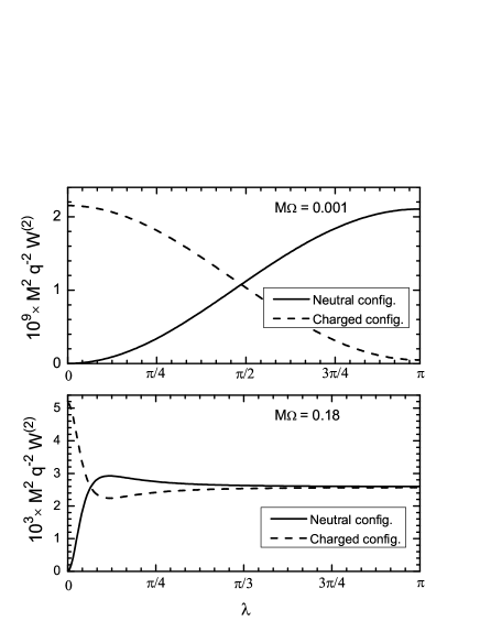
Figure 3: The total power (23) is plotted as a function of the angular separation $\lambda$ for neutral and charged configurations for small ($M\Omega=0.001$) and large ($M\Omega=0.18$) angular velocities. In the small $\Omega$ case, the curves are roughly sinusoidal which is typical for dipole emission ($l=m=1$), while in the large $\Omega$ case, the curves present a non-monotonic behavior because of the significant contribution coming from higher multipoles. Here, Eqs. (9)-(10) and (11)-(12) were used for $\psi^{\alpha}_{\omega l}$ in the top and bottom graphs, respectively.

In Fig. 3, we plot the total power $W^{(2)}$ as a function of $\lambda$ assuming neutral and charged configurations for the cases where the sources have small ($M\Omega\ll M\Omega_{\gamma}\approx 0.19$) and large ($M\Omega\lesssim M\Omega_{\gamma}\approx 0.19$) angular velocities. In the small $\Omega$ case, the curves are seen to be roughly proportional to $1\pm\cos\lambda$ following a dipole pattern CED . This is not so, however, in the large $\Omega$ case, where the various multipole contributions drive the curves to become nontrivial. We note, in particular, that interference effectively vanishes for large enough $\lambda$ in this case (in the sense that the various multipole terms combine in such a way that both sources emit as if they were independent from each other), driving charged and neutral configurations to behave similarly.

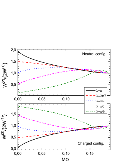
Figure 4: The ratio between the total power emitted by the two-source system and twice the total power emitted by a single source, $W^{(2)}/(2W^{(1)})$, is plotted as a function of $\Omega$ for several angular separations $\lambda$. As $\Omega$ approaches $\Omega_{\gamma}$ ($M\Omega_{\gamma}\approx 0.19$), this ratio goes to $1$ for every $\lambda$, implying that distinct sources emit irrespectively to each other for large enough $\Omega$. Here, Eqs. (11)-(12) were used for the radial functions.

Interference effects are expected to be important when the typical radiation wavelength $1/\omega_{\rm typ}$ is of order or larger than the distance $\lambda R$ between the sources. This leads to the following interference condition:

$$m_{\rm typ}\lesssim[\lambda(M\Omega)^{1/3}]^{-1},$$

where we have used that $\omega_{\rm typ}=\Omega\,m_{\rm typ}$ and $R=(M/\Omega^{2})^{1/3}$. Thus, for sources with $\Omega\lesssim\Omega_{\gamma}$ (i.e., at $R\gtrsim 3M$), Eq. (24) implies that we should not expect interference unless the sources are quite close to each other. Fig. 4 exhibits the $W^{(2)}/(2W^{(1)})$ ratio as a function of $\Omega$ for several angular separations $\lambda$, where we recall that $W^{(2)}$ denotes the total power emitted by the two-source system as given by Eq. (23), while $2W^{(1)}$ is twice the total power emitted by a single source. (We fix $\Omega$ to be the same in both cases.) Deviations from the unity indicate constructive ($W^{(2)}/(2W^{(1)})>1$) and destructive ($W^{(2)}/(2W^{(1)})<1$) interference. We can see from this graph how $W^{(2)}/(2W^{(1)})$ approaches the unity as $\Omega$ gets closer to $\Omega_{\gamma}$ and interference tends to effectively vanish.

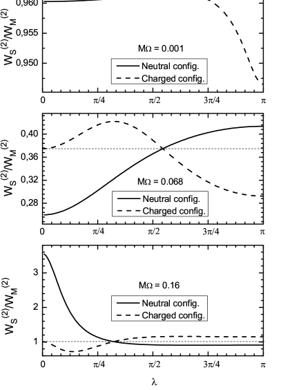
Figure 5: The $W^{(2)}_{\rm S}/W^{(2)}_{\rm M}$ ratio is plotted as a function of the angular separation $\lambda$ for $M\Omega=0.001,0.68,0.16$. The horizontal dashed lines correspond to $W^{(1)}_{\rm S}/W^{(1)}_{\rm M}$. The variation of $W^{(2)}_{\rm S}/W^{(2)}_{\rm M}$ with respect to $W^{(1)}_{\rm S}/W^{(1)}_{\rm M}$ indicates the influence of the spacetime curvature on interference and is seen to increase in a non-trivial way as $\Omega$ approaches $\Omega_{\gamma}$.

In order to investigate the role played by the spacetime curvature on interference, we must compare $W^{(2)}/(2W^{(1)})$ as calculated in Schwarzschild (S) and Minkowski (M) spacetimes, namely:

$$\frac{W_{\rm S}^{(2)}/(2W_{\rm S}^{(1)})}{W_{\rm M}^{(2)}/(2W_{\rm M}^{(1)})}=\frac{W_{\rm S}^{(2)}/W_{\rm M}^{(2)}}{W_{\rm S}^{(1)}/W_{\rm M}^{(1)}},$$ (26)

where $W^{(1)}_{\rm M}$ is the total power emitted by a single source as computed in Minkowski spacetime assuming Newtonian gravity. In this case, we relate the angular velocity $\Omega$ with the radial coordinate $R$ using the Kepler law, which formally reads as in Eq. (18) although we should keep in mind that in the flat spacetime case all quantities refer to Cartesian coordinates rather than to Schwarzschild ones. $W^{(2)}_{\rm M}$ is defined accordingly for a two-source system. Rather than plotting Eq. (26), we exhibit in Fig. 5 $W_{S}^{(2)}/W_{M}^{(2)}$ and $W_{S}^{(1)}/W_{M}^{(1)}$ separately as functions of $\lambda$ for various $\Omega$ values assuming charged and neutral configurations. $W_{S}^{(1)}/W_{M}^{(1)}$ (dotted horizontal lines) carries information about the curvature influence on the radiation emitted by single sources and obviously does not depend on $\lambda$ , while $W_{S}^{(2)}/W_{M}^{(2)}$ carries information about the curvature influence on interference as discussed in the context of Eq. (26). This is interesting to note that the term $1\pm\cos(m\lambda)$ codifying the $\lambda$ dependence in Eq. (23) is the same in Minkowski and Schwarzschild spacetimes because the angular structure of the corresponding metrics (which is the relevant feature here) is identical in both cases. The nontriviality of Fig. 5 comes from the fact that as one computes the total power, the sum in the quantum number $m$ couples the $1\pm\cos(m\lambda)$ term to the radial functions, which are distinct in the curved and flat spacetimes. For low enough angular velocities (see $M\Omega=0.001$), only the $l=1$ contribution is relevant and such coupling is “weak”. This is reflected in a small variation of the $W_{\rm S}^{(2)}/W_{\rm M}^{(2)}$ curve with respect to $W_{\rm S}^{(1)}/W_{\rm M}^{(1)}$ (horizontal dashed line) in the whole $\lambda$ domain (note the scale). Now, as $\Omega$ increases (see $M\Omega=0.068,0.16$), larger values of angular momenta are excited and the behavior of $W_{\rm S}^{(2)}/W_{\rm M}^{(2)}$ becomes nontrivial. Thus, despite the fact that the same $1\pm\cos(m\lambda)$ dependence appears in Schwarzschild and Minkowski cases, the coupling of this term to the proper radial functions generates a non-trivial interplay between spacetime geometry and interference.

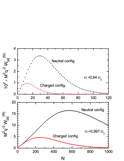
Figure 6: The total power $W^{(N)}_{[a]}$ is plotted as a function of $N$ for two orbits in the high-frequency regime, corresponding to $\Omega\approx 0.94\Omega_{\gamma}$ and $\Omega\approx 0.997\Omega_{\gamma}$. As $N\to\infty$, $W^{(N)}_{[a]}\to 0$ and we recover the non-radiating limit. Here, Eqs. (11)-(12) were used for $\psi^{\alpha}_{\omega l}(x)$.

III.2 $N$ scalar sources

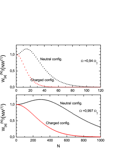
Figure 7: The $W_{[a]}^{(N)}/(NW^{(1)})$ ratio is plotted as a function of $N$ for $\Omega\approx 0.94\Omega_{\gamma}$ and $\Omega\approx 0.997\Omega_{\gamma}$. We note the existence of a region of constructive interference in the neutral case that is not present for the charged configuration. Here, Eqs. (11)-(12) were used for $\psi^{\alpha}_{\omega l}(x)$.

In this section we are interested in investigating the transition from the radiating to the non-radiating regime as the number of sources $N$ increases. They are assumed to be free and orbit the black hole with same angular velocity $\Omega$ ($r=R$). The $N$-source system will be described by

$$j_{[+]}(x^{\mu}) = \sum_{n=1}^{N}\frac{q}{\sqrt{-g}u^{0}}\delta(r-R)\delta(\theta-\pi/2)$$ (27)

$$\times \delta(\varphi-\Omega t-(n-1)\lambda)$$

and

$$j_{[0]}(x^{\mu}) = \sum_{n=1}^{N}\frac{q(-1)^{n-1}}{\sqrt{-g}u^{0}}\delta(r-R)\delta(\theta-\pi/2)$$ (28)

$$\times \delta(\varphi-\Omega t-(n-1)\lambda).$$

for charged and neutral configurations, respectively, where $\lambda=2\pi/N$, i.e. the sources are equally spaced around the orbit. In the charged configuration, all sources have the same coupling $q$, while in the neutral one sources with $+q$ and $-q$ appear alternately around the orbiting circle ($N$ is assumed even here).

The total power $W^{(N)}_{[a]}$ ($a=+,0$) emitted by these $N$-source systems can be calculated:

$$W_{[a]}^{(N)}(\Omega)=\sum_{\alpha=\rightarrow}^{\leftarrow}\sum_{l=1}^{\infty}\sum_{m=1}^{l}W^{(1)}_{\alpha lm}(\Omega)g_{[a]m}^{(N)},$$ (29)

where $W^{(1)}_{\alpha lm}$ is given in Eq. (25) and the interference factor can be cast as

$$g^{(N)}_{[+]m}=\left\{\begin{array}[]{lllll}N^{2}&{\rm when}&m=kN&{\rm for\,some}&k\in\mathbb{N}\\ 0&{\rm when}&m\neq kN&{\rm for\,every}&k\in\mathbb{N}\end{array}\right.$$ (30)

and

$$g^{(N)}_{[0]m}=\left\{\begin{array}[]{lllll}N^{2}&{\rm when}&m=(2k-1)N/2&{\rm for\,some}&k\in\mathbb{N}\\ 0&{\rm when}&m\neq(2k-1)N/2&{\rm for\,every}&k\in\mathbb{N}\end{array}\right.$$ (31)

in the charged and neutral cases, respectively. As discussed in Fig. 2, the largest values acquired by $W^{(1)}_{lm}\equiv\sum_{\alpha}W^{(1)}_{\alpha lm}$ happen for $l=m\approx m_{\rm typ}$ [see Eq. (24)]. The role played by $g^{(N)}_{[a]m}$ is twofold: on one hand, it increases the power by a factor of $N^{2}$ and, on the other one, it restricts the sum in Eq. (29) to just a few significant terms: $m=N,2N,...$ for the charged configuration and $m=N/2,3N/2,...$ for the neutral one. Thus, for low angular velocities (in which case only small multipoles are relevant) the emitted total power goes quickly to zero as the number of sources $N$ increases. Notwithstanding, if $\Omega\lesssim\Omega_{\gamma}$, higher multipoles get important and the power radiated by a larger number of sources can be significant. In Fig. 6, we show the total emitted power $W^{(N)}_{[a]}$ as a function of $N$ for two angular velocities in the high-frequency regime assuming neutral and charged configurations. We note that, as the orbit approaches the innermost circular geodesic, the number of sources which maximize the emitted power increases as well as the range of $N$ for which emission is significant. We also note that, for a given $N$, the neutral configuration radiates typically more than the charged one. For large enough $N$, however, interference takes control damping the emitted radiation.

In Fig. 7, we compare the total emitted power $W^{(N)}_{[a]}$ with $N$ times the total power emitted by a single source $W^{(1)}$ for two angular velocities in the high-frequency regime assuming neutral and charged configurations by plotting $W^{(N)}_{[a]}/(NW^{(1)})$. For small enough $N$, we see that $W^{(N)}_{[a]}/(NW^{(1)})\approx 1$, indicating that the contribution coming from each source is mostly independent from each other. As $N\to\infty$, however, interference becomes important and we recover the non-radiating regime. It is also interesting to note from Fig. 7 the existence of a region in which interference is constructive ($W^{(N)}/(NW^{(1)})>1$) for the neutral configuration in contrast to the charged case.

The fact that interference effects should become important when the wavelengths of the emitted waves (of the order $1/\omega_{\rm typ}$) are larger than the distance $2\pi R/N$ between the sources allows us to estimate the number $\bar{N}$ above which interference cannot be neglected:

$$\bar{N}\approx 2\pi\frac{M(1-2M/R)}{R(1-3M/R)}.$$ (32)

For the angular velocities considered in Figs. 6 and 7, $\bar{N}=17$ and $350$ for $\Omega=0.94\,\Omega_{\gamma}$ and $\Omega=0.997\,\Omega_{\gamma}$, respectively.

IV Final Remarks

We have considered the radiation emitted by an ensemble of scalar sources in circular geodesic orbits around a Schwarzschild black hole. Interference associated with the emitted radiation was investigated and particular attention was given to the role played by the spacetime curvature. The non-radiating regime is recovered as the number of sources $N$ increases. Finally, a simple useful result can be derived as follows: the power emitted by a scalar source following ultrarelativistic circular orbits in Schwarzschild spacetime can be estimated to be

$$W_{\delta}^{(1)}\approx 10^{-4}(q/M)^{2}\delta^{-1},$$ (33)

when $R\equiv(3+\delta)M$ and $0<\delta\ll 1$. As a consequence, we get that the total emitted power associated with $N$ sources will be $W^{(N)}_{[a]}\approx NW_{\delta}^{(1)}$ for $N\ll\bar{N}$ and $W^{(N)}_{[a]}\approx 0$ for $N\gg\bar{N}$.

The radiation component coming from the collective rotational motion of charges in highly ionized accretion disks orbiting black holes should be mostly damped by interference effects as the disk lies in the $R>6M$ region. However, in the short time interval which charges spend at $R<6M$, the role played by interference should decrease as highly energetic radiation is emitted, in accordance with our results.

References

• (1) W. Lewin and M. van der Klis, Compact Stellar X-ray Sources (Cambridge University Press, Cambridge, 2006). R. Genzel, F. Eisenhauer, and S. Gillessen, Rev. Mod. Phys., 82, 3121 (2010).
• (2) C. W. Misner, R. A. Breuer, D. R. Brill, P. L. Chrzanowski, H. G. Hughes III and C. M. Pereira, Phys. Rev. Lett. 28, 998 (1972). R. A. Breuer, P. L. Chrzanowski, H. G. Hughes III and C. W. Misner, Phys. Rev. D 8, 4309 (1973).
• (3) R. A. Breuer, Gravitational Perturbation Theory and Synchrotron Radiation - Lecture Notes in Physics (Springer-Verlag, Heidelberg, 1975).
• (4) E. Poisson, Phys. Rev. D 52, 5719 (1995).
• (5) L. C. B. Crispino, A. Higuchi and G. E. A. Matsas, Class. Quantum Grav. 17, 19 (2000).
• (6) L. M. Burko, Phys. Rev. Lett. 84, 4529 (2000).
• (7) V. Cardoso and J. P. S. Lemos, Phys. Rev. D 65, 104033 (2002).
• (8) J. Castiñeiras, L. C. B. Crispino, R. Murta and G. E. A. Matsas, Phys. Rev. D 71, 104013 (2005).
• (9) L. C. B. Crispino, A. R. R. da Silva and G. E. A. Matsas, Phys. Rev. D 79, 024004 (2009).
• (10) N. D. Birrel and P. C. W. Davies, Quantum Fields in Curved Space (Cambridge University Press, Cambridge, 1982).
• (11) C. Itzykson and J.-B. Zuber, Quantum Field Theory (McGraw-Hill, New York, 1980).
• (12) I. S. Gradshteyn and I. M. Ryzhik, Tables of Integrals, Series, and Products (Academic Press, New York, 1980).
• (13) J. D. Jackson, Classical Electrodynamics 2nd edn (New York: Wiley, 1975).
• (14) A. Higuchi, G. E. A. Matsas and D. Sudarsky, Phys. Rev. D 58, 104021 (1998).