A Modulus-Squared Dirichlet Boundary Condition for Time-Dependent Complex Partial Differential Equations and its Application to the Nonlinear Schrödinger Equation

Abstract

An easy to implement modulus-squared Dirichlet (MSD) boundary condition is formulated for numerical simulations of time-dependent complex partial differential equations in multidimensional settings. The MSD boundary condition approximates a constant modulus-square value of the solution at the boundaries. Application of the MSD boundary condition to the nonlinear Schrödinger equation is shown, and numerical simulations are performed to demonstrate its usefulness and advantages over other simple boundary conditions.

1 Introduction

When utilizing numerical methods to approximate the solutions to time-dependent partial differential equations (PDEs), proper handling of boundary conditions can be quite challenging. Sometimes, an otherwise stable numerical scheme will become unstable depending on how the boundary conditions are computed [1]. In addition, high-order schemes can degrade in accuracy to lower-order when using boundary conditions which are not compatible with the high-order accuracy [2]

Often, researchers will forgo a complicated boundary condition implementation and instead use tried-and-true boundary conditions techniques which are very simple yet provide acceptable results. One of the most common is the use of Dirichlet boundary conditions, where the function value at the boundary of the domain is set to a constant value (commonly this value is zero). A Dirichlet boundary condition of zero-value is often used when simulating solutions which decay towards zero at infinity, and where most of the dynamics (or ‘action’) is expected to remain in the central regions of the computational grid.

Problems involving PDEs whose function values are complex cannot, in general, make use of standard Dirichlet boundary conditions because of the constant oscillation of the real and imaginary parts of the function due to the intrinsic frequency of the system and the dynamics of the solutions (when the solution decays to zero at infinity, standard Dirichlet conditions of zero-value can be used). There are situations (for examples, see Sec. 4) where the modulus-squared of the solution converges to a constant value at the boundary. In such a case, a modulus-squared Dirichlet (MSD) boundary condition (which keeps the modulus-squared of the solution at the boundaries constant) would be desirable.

In this paper, we present a simple way to simulate a modulus-squared Dirichlet boundary condition in time-dependent complex-valued PDEs. The MSD boundary condition is very easy to implement and has an accuracy equal to the interior numerical scheme (as long as the assumption of a constant modulus-squared value at the boundary is valid). This new boundary condition eliminates the need for overly large grids or expensive and complicated boundary conditions for many problems.

A very common time-dependent complex-valued PDE used in a wide range of applications is the nonlinear Schrödinger equation (NLSE). The NLSE is a universal model describing the evolution and propagation of complex filed envelopes in nonlinear dispersive media. As such, it is used to describe many physical systems [3] including nonlinear optics [4] and the mean-field dynamics of Bose-Einstein condensates (BECs) (in which case the NLSE is typically modified to include an external potential term, in which case the NLSE is referred to as the Gross-Pitaevskii equation) [5]. In systems such as optics and BECs, the modulus-squared of the solution (referred to as the ‘wavefunction’) represents the observable (intensity of light and atomic density respectively). In this situation, often the dynamics of ‘dark’ structures (dark solitons, vortices, vortex lines, vortex rings, etc.) which reside inside medium are studied. These are coherent structures of very low (or zero) central density which exist inside the bulk of the medium. The most basic form of the structures can be examined by assuming an infinite-extent domain, in which case the solutions exist within an infinite constant-density background. Such a situation is very well-suited for the use of MSD boundary conditions. As such, in Sec. 4, we use simulations of dark coherent structures in the NLSE to test the MSD boundary condition.

Many sophisticated boundary conditions have been developed for both the linear and nonlinear Schrödinger equations which simulate transparent or artificial boundaries (see the review of Ref. [6] and references therein). Most of these boundary conditions focus on eliminating reflections off the boundaries (the biggest problem when using Dirichlet boundary conditions) when studying dynamics which trail off to zero at infinity. Since our main concern are boundary conditions in a constant-density scenario, we do not make use of the boundary conditions described there. Additionally, one of the main features of the MSD boundary condition is that its simplicity of implementation allows small research projects to make common use of them. The boundary conditions shown in Ref. [6] can be very complicated to implement, and are therefore best suited for large projects.

The paper is organized as follows: In Sec. 2 we formulate the MSD boundary condition in general for any time-dependent complex-valued PDE. Then, in Sec. 3, we apply the MSD boundary condition to the NLSE. In Sec. 4 we numerically test the MSD boundary condition for simulating the NLSE using a Runge-Kutta finite-difference scheme. Stability effects when using the MSD boundary condition are discussed in Sec. 5. We conclude in Sec. 6.

2 Formulation of the MSD Boundary Condition

2.1 Notation

For this paper we use the notation $\Psi_{b}$ to describe the grid-points on a boundary and $\Psi_{b-1}$ to describe the grid-points one cell in from the boundary in the normal direction to the boundary points (i.e. in two-dimensions, the top-left corner point would be a $\Psi_{b}$ and the point one cell to the right and and one cell down would be $\Psi_{b-1}$). We denote the real part of $\Psi$ as $\Psi^{R}$ and the imaginary part as $\Psi^{I}$. We also use the notation $\Psi_{\alpha}$ to denote the first derivative with respect to $\alpha$ ($\partial\Psi/\partial\alpha$), and so $\Psi_{\alpha,b}$ would refer to the first partial derivative with respect to $\alpha$ at the boundary points, where $\alpha$ can represent a spatial ($x$) or temporal ($t$) dependence.

2.2 Derivation of the MSD boundary Condition

We start out by stating the condition, that for all times, the modulus-squared of the function $\Psi$ at the boundaries is equal to a constant, positive, real value $B$,

$$|\Psi_{b}|^{2}=B.$$ (1)

In such a case we have that

$$\frac{\partial}{\partial t}\,|\Psi_{b}|^{2}=0,$$

and thus

$$\frac{\partial}{\partial t}\,\left(\Psi_{b}^{R}\right)^{2}+\frac{\partial}{\partial t}\,\left(\Psi_{b}^{I}\right)^{2}=0.$$ (2)

By using the chain rule and rearranging, Eq. (2) is equivalent to

$$\Psi_{b}^{R}\,\frac{\partial\Psi_{b}^{R}}{\partial t}=-\Psi_{b}^{I}\,\frac{\partial\Psi_{b}^{I}}{\partial t}.$$ (3)

A non-trivial solution that satisfies Eq. (3) is given by

$$\frac{\partial\Psi_{b}^{R}}{\partial t}=C\,\Psi_{b}^{I}\qquad\mbox{and}\qquad\frac{\partial\Psi_{b}^{I}}{\partial t}=-C\,\Psi_{b}^{R},$$ (4)

where $C$ is a constant. Since $\Psi_{t,b}=\Psi_{b,t}^{R}+i\,\Psi_{b,t}^{I}$, Eq. (4) can be expressed as

$$\Psi_{b}=\frac{i}{C}\,\Psi_{t,b}.$$ (5)

Eq. (5) gives the form of the MSD boundary condition on $\Psi_{t}$ in terms of the boundary point $\Psi_{b}$ and the constant $C$. In order to find the correct value of $C$, we differentiate Eq. (5) in the normal direction to the boundary (here represented as the $x$-direction) to get

$$\frac{\partial}{\partial x}\Psi_{b}=\frac{i}{C}\,\frac{\partial}{\partial x}\Psi_{t,b}.$$ (6)

Discretizing the spatial derivatives of Eq. (6) using forward-differencing yields

$$\frac{\Psi_{b-1}-\Psi_{b}}{h}-\frac{h}{2}\Psi_{xx,b}+O(h^{2})=\frac{i}{C}\left[\frac{\Psi_{t,b-1}-\Psi_{t,b}}{h}-\frac{h}{2}\Psi_{txx,b}+O(h^{2}).\right],$$ (7)

where $h$ is the grid spacing between the boundary and the interior point in the normal direction. Inserting Eq. (5) into Eq. (7) to eliminate temporal derivatives at the boundary points yields

$$\frac{\Psi_{b-1}-\Psi_{b}}{h}-\frac{h}{2}\Psi_{xx,b}+O(h^{2})=\frac{i}{C}\left[\frac{\Psi_{t,b-1}+i\,C\Psi_{b}}{h}+\frac{i\,h\,C}{2}\Psi_{xx,b}+O(h^{2}).\right].$$ (8)

It is observed that the truncation terms shown in Eq. (8) cancel out, and by the same formulation, all the additional truncation terms will also cancel out. Therefore, we have

$$\frac{\Psi_{b-1}-\Psi_{b}}{h}=\frac{i}{C}\left[\frac{\Psi_{t,b-1}+i\,C\Psi_{b}}{h}\right],$$ (9)

which yields the expression for $C$ given by

$$C=i\,\frac{\Psi_{t,b-1}}{\Psi_{b-1}}.$$ (10)

Eq. (10) is computable since the value of $\Psi_{t,b-1}$ is computed using using the interior scheme being implemented. Inserting the value of $C$ of Eq. (10) into the MSD boundary condition formulation of Eq. (5) yields

$$\Psi_{t,b}\approx\frac{\Psi_{t,b-1}}{\Psi_{b-1}}\,\Psi_{b}.$$ (11)

The MSD boundary condition of Eq. (11) can be obtained in an alternative way by noting that a steady-state (in the modulus-squared) of a complex time-dependent function can be given as

$$\Psi=|\Psi|\,\mbox{exp}(-i\,\Omega\,t),$$

where $\Omega$ is the frequency and $|\Psi|$ is the constant-valued amplitude of $\Psi$. If we assume that this relationship is true at the boundary points of the grid, we have

$$\frac{\partial\Psi_{b}}{\partial t}=-i\,\Omega_{b}\,|\Psi_{b}|\,\mbox{exp}(i\,\Omega_{b}\,t)=-i\,\Omega_{b}\,\Psi_{b}.$$ (12)

From Eq. (12), we get

$$\Omega_{b}=i\,\frac{\Psi_{t,b}}{\Psi_{b}}.$$ (13)

Assuming that the closest interior grid point is nearly steady-state, we can infer that

$$\Omega_{b-1}\approx i\,\frac{\Psi_{t,b-1}}{\Psi_{b-1}}.$$ (14)

If it is assumed that the frequency of the interior point is approximately equal to the frequency at the boundary (i.e. $\Omega_{b}\approx\Omega_{b-1}$), then by inserting Eq. (14) as $\Omega_{b}$ in Eq. (12), Eq. (12) becomes the MSD boundary condition of Eq. (11).

This formulation of the MSD boundary condition shows that the $\Psi_{t,b}/\Psi_{b}$ term in Eq. (11) should be equal to $i$ times the frequency. Since the frequency of the solution is a real value, computing $\Psi_{t,b-1}/\Psi_{b-1}$ may introduce a small imaginary part to the frequency due to numerical errors. This would lead the solution at the boundaries to undergo exponential growth. In order to ensure that the computed frequency is real-valued (i.e. that $\Psi_{t,b-1}/\Psi_{b-1}$ is purely imaginary), we modify the MSD boundary condition of Eq. (11) to be

$$\Psi_{t,b}\approx i\,\mbox{Im}\left[\frac{\Psi_{t,b-1}}{\Psi_{b-1}}\right]\,\Psi_{b}.$$ (15)

When using the MSD boundary condition in programming environments that do not intrinsically handle complex variables, Eq. (15) must be explicitly split into its real and imaginary parts. We begin by expanding the unmodified MSD boundary condition of Eq. (11) into its real and imaginary parts, given by

$$\Psi_{t,b}^{R}+i\,\Psi_{t,b}^{I}\approx\frac{\Psi_{t,b-1}^{R}+i\,\Psi_{t,b-1}^{I}}{\Psi_{b-1}^{R}+i\,\Psi_{b-1}^{I}}\left(\Psi_{b}^{R}+i\,\Psi_{b}^{I}\right).$$

which leads to

$$\Psi_{t,b}^{R}+i\,\Psi_{t,b}^{I}\approx\left[\frac{\Psi_{t,b-1}^{R}\,\Psi_{b-1}^{R}+\Psi_{t,b-1}^{I}\,\Psi_{b-1}^{I}}{\left(\Psi^{R}_{b-1}\right)^{2}+\left(\Psi^{I}_{b-1}\right)^{2}}+i\,\left(\frac{\Psi_{t,b-1}^{I}\,\Psi_{b-1}^{R}-\Psi_{t,b-1}^{R}\,\Psi_{b-1}^{I}}{\left(\Psi^{R}_{b-1}\right)^{2}+\left(\Psi^{I}_{b-1}\right)^{2}}\right)\right]\,\left(\Psi_{b}^{R}+i\,\Psi_{b}^{I}\right).$$ (16)

Going back to Eq. (3), we see that the first term in the brackets of Eq. (16) is equal to zero at the boundary. If it is assumed that the interior points are similar, the term can be dropped. Dropping the term is equivalent to the numerical fix used in Eq. (15), ensuring that the frequency of the solution $\Psi$ at the boundary is real-valued. Simplifying Eq. (16) with this in mind yields the separated MSD boundary condition

$$\Psi^{R}_{t,b} =-\tilde{\Omega}\,\Psi^{I}_{b}$$ (17)

$$\Psi^{I}_{t,b} =\tilde{\Omega}\,\Psi^{R}_{b},$$

where

$$\tilde{\Omega}=\frac{\Psi^{I}_{t,b-1}\,\Psi^{R}_{b-1}-\Psi^{R}_{t,b-1}\,\Psi^{I}_{b-1}}{\left(\Psi^{R}_{b-1}\right)^{2}+\left(\Psi^{I}_{b-1}\right)^{2}}.$$ (18)

The MSD boundary condition of Eqs. (15), (17), and (18) is given for the temporal derivative of the boundary point. This is ideally suited for Runge-Kutta type solvers, as the right hand side of the PDEs ($\Psi_{t}$) are evaluated and used for the time-stepping [7]. For other methodologies, or in situations where the boundary value of the spatial derivatives is needed, the MSD boundary condition can be inserted into the governing equation to formulate the required boundary conditions. An example of this is shown in Sec. 3 for the NLSE.

In situations where the sequential computation of the internal scheme followed by the boundary condition computations is not appropriate (for example, implicit finite-difference schemes) one can substitute the internal scheme of $\Psi_{t,b-1}$ into Eq. (11) and implement the boundary condition concurrently with the internal scheme (this would add extra computational steps as $\Psi_{t,b-1}$ would essentially be computed twice). Alternatively, if the frequency, $\Omega$, of the overall solution is known, the $\Psi_{t,b-1}/\Psi_{b-1}$ term can be replaced with $i\,\Omega$ directly as shown above.

If it happens that $\Psi_{b-1}=0$, the MSD boundary condition of Eq. (11) has a singularity. However, in most situations, $\Psi_{b-1}$ only takes a zero value when the solution is tending toward zero at the boundary. In that case, the standard Dirichlet boundary condition of $\Psi_{b}=0$ can be used instead of the MSD boundary condition.

2.3 Key Features of the MSD Boundary Condition

The following are a few key features of the MSD boundary condition:

• The formulation of the MSD boundary condition does not depend at all on the specific PDE being simulated, only that it is time-dependent, and is complex-valued.

• The MSD boundary condition can be used in multidimensional settings without modification since each boundary point only uses one interior point in the normal direction to the boundary.

• The MSD boundary condition does not depend on the size of the grid spacing, and therefore does not need to be altered when using unequal grid spacing (for example, in adaptive mesh refinement applications).

• The MSD boundary condition can be considered compact, in that after computing the internal scheme, the boundary values only depend on their nearest neighboring grid point. This allows the MSD boundary condition to be easily implemented in parallel environments.

• In general, the MSD boundary condition is extremely easy to implement (see Appendix A for MATLAB code showing an implementation of the MSD boundary condition in one-dimension). This makes the MSD boundary condition an attractive alternative to more complicated boundary condition methodologies.

3 Application of the MSD boundary condition to the NLSE

Here we show an implementation of the MSD boundary condition for the NLSE. The NLSE with an external potential can be given in general form as

$$i\,\frac{\partial\Psi}{\partial t}+a\,\nabla^{2}\Psi-V({\bf r})\,\Psi+s\,|\Psi|^{2}\,\Psi=0,$$ (19)

where $\Psi$ is the wavefunction, $V({\bf r})$ is an external potential, and $a$ and $s$ are parameters determined by the physical system being modeled.

As mentioned in Sec. 2.2, since the MSD boundary condition of Eq. (15) is given in terms of the temporal derivative, it is well suited for Runge-Kutta schemes, in which case it can be applied directly. However, other numerical schemes require boundary conditions on the Laplacian operator itself. This can be worked out by inserting Eq. (19) into Eq. (15) yielding

$$\nabla^{2}\Psi_{b}\approx\left[\mbox{Im}\left(i\,\frac{\nabla^{2}\Psi_{b-1}}{\Psi_{b-1}}\right)+\frac{1}{a}\,\left(N_{b-1}-N_{b}\right)\right]\Psi_{b},$$ (20)

where

$$N_{b}=s\,|\Psi_{b}|^{2}-V_{b},\qquad N_{b-1}=s\,|\Psi_{b-1}|^{2}-V_{b-1}.$$ (21)

Splitting Eq. (20) into real and imaginary parts yields

$$\nabla^{2}\Psi^{R}_{b} \approx\left[A+\frac{1}{a}\left(N_{b-1}-N_{b}\right)\right]\,\Psi^{R}_{b},$$ (22)

$$\nabla^{2}\Psi^{I}_{b} \approx\left[A+\frac{1}{a}\left(N_{b-1}-N_{b}\right)\right]\,\Psi^{I}_{b},$$

where

$$A=\frac{\nabla^{2}\Psi^{R}_{b-1}\,\Psi^{R}_{b-1}+\nabla^{2}\Psi^{I}_{b-1}\,\Psi^{I}_{b-1}}{\left(\Psi^{R}_{b-1}\right)^{2}+\left(\Psi^{I}_{b-1}\right)^{2}},$$ (23)

and $N_{b-1}$ and $N_{b}$ are as defined in Eq. (21).

As discussed in Sec. 2.2 the MSD boundary condition can be expanded out, expressing the $b-1$ Laplacian in terms of the internal scheme in order to be able to evaluate the MSD boundary condition simultaneously with the interior points. (When using explicit time-stepping schemes, this is usually unnecessary). As an example, using central-differencing in space for the one-dimensional NLSE, Eq. (20) becomes

$$\nabla^{2}\Psi_{b}\approx\left[\mbox{Im}\left(i\,\frac{\Psi_{b}+\Psi_{b-2}}{\Psi_{b-1}}\right)-2+\frac{1}{a}\,\left(N_{b-1}-N_{b}\right)\right]\Psi_{b},$$ (24)

where $N_{b-1}$ and $N_{b}$ are as defined in Eq. (21).

4 Numerical Results

In order to demonstrate the usefulness and advantages of the MSD boundary condition, we show a few example simulations of the NLSE. The MSD boundary condition is compared to a Laplacian-zero (L0) boundary condition defined as $\nabla^{2}\Psi_{b}=0$. The Laplacian-zero boundary condition is chosen for comparison because it is an easy-to-implement boundary condition that is possible to use for constant background-density simulations in specific cases.

Each boundary condition, including the MSD, are only valid given their own assumptions. Therefore if the modulus-squared of a solution is changing at the boundary, the MSD is not expected to work well, just as if the Laplacian of the wavefunction is far from zero at the boundary, the Laplacian-zero boundary condition is not expected to do well. Therefore, comparisons of which boundary condition is best is very often problem-specific. That being said, comparing the MSD to the L0 is still valuable in that for some problems, both boundary conditions are suitable allowing for a fair comparison and, in addition, since limiting the size of the required grid is very important (especially for higher-dimensional simulations), it is useful to see which boundary condition allows for the use of the smallest (tightest) grid within acceptable accuracy limits.

While there are numerous numerical methods that can be used to simulate solutions to the NLSE, we choose to perform the simulations using the code package NLSEmagic [8] which uses the fourth-order in time Runge-Kutta method with second-order central-differencing in space (RK4+CD).

4.1 One-Dimensional Dark Solitons in the NLSE

For the one-dimensional tests, a co-moving dark soliton solution with $V({\bf r})=0$ is used, given by [5]

$$\Psi(x,t)=\sqrt{\frac{\Omega}{s}}\,\mbox{tanh}\left[\sqrt{\frac{\Omega}{2a}}\,(x-c\,t)\right]\,\mbox{exp}\left(i\left[\frac{c}{2a}\,x+\left(\Omega-\frac{c^{2}}{4a}\right)t\right]\right)$$ (25)

where $c$ is the velocity of the soliton and $\Omega$ is a chosen parameter representing the frequency of the solution.

The first test is to compare the error for a steady-state dark soliton with $c=0$. In such a case, for a large enough domain, the L0 boundary condition can be used since $\Psi$ flattens out at infinity. In contrast, the MSD boundary condition should work on any sized domain, since its underlying assumption of constant density is valid anywhere along the steady-state solution. A one-sided second-order differencing (1SD) boundary condition defined in one-dimension as

$$\frac{\partial^{2}\Psi}{\partial x^{2}}\approx\frac{1}{h^{2}}\,\left(-\Psi_{b-3}+4\,\Psi_{b-2}-5\,\Psi_{b-1}+2\,\Psi_{b}\right),$$

is also used for comparison in this case.

We define a radius, $r$, which represents the distance from the center of the soliton to the edge of the computational domain. Simulations are performed for various lengths of $r$ ranging from $r=5$ (approximately equal to the width of the soliton) to $r=25$ (the distance where the boundary value of the soliton is approximately equal to the infinite background density minus machine epsilon $\epsilon\approx 10^{-16}$). The average of the maximum errors in the real and imaginary part of $\Psi$ over the length of the simulations are recorded. The results are shown in Fig. 1.

$\begin{array}[]{cc}\includegraphics[width=224.03743pt]{MSD_1D_c0_T50_k006_h01_r5-25_f100}&\includegraphics[width=224.03743pt]{MSD_1D_c0_T50_k006_h01_r5-25_f100_SOL}\end{array}$

Figure 1: Left: Comparisons of errors for simulating the dark-soliton solution (with $c=0$, $\Omega=-1$, $a=1$, and $s=-1$) of Eq. (25) using MSD (blue dashed line), L0 (red squares), 1SD (green dots), and exact (black solid line) boundary conditions for various domain sizes. The simulations are run to an end time of $t=50$ with a time-step of $k=0.006$ and spatial step of $h=0.1$. Right: Depiction of the soliton for the maximum domain ($r=25$) simulation at time $t=50$. The dashed (blue) and dotted (red) lines are the real and imaginary parts of $\Psi$ respectively, while the solid line is the modulus-squared, $|\Psi|^{2}$. The definition of the radius $r$ in the error plots is illustrated.

Keeping in mind that $h^{2}=10^{-2}$ and the spatial scheme is $O(h^{2})$, it is clear that the MSD boundary condition performs well even when the domain is small. Both the L0 and the MSD boundary conditions outperform the 1SD boundary condition. It is understandable that the L0 boundary condition out-performs the MSD when $r$ get large, as the Laplacian tends towards zero rapidly as $r$ increases, and the L0 boundary condition has no additional error associated with it. Even so, the MSD can simulate the solution at a smaller grid size than the L0 can to acceptable accuracy, demonstrating its usefulness in this case.

For the next test, the soliton is given a velocity of $c=0.5$. Since the L0 assumptions are completely invalid at any domain size, it is not used for comparison (the 1SD is also not used as it fails quickly at any domain size as well). Therefore, the MSD boundary condition is only compared to the exact boundary condition. In this case the domain is set to be a distance $r$ to the left of the initial position of the soliton, and a distance $r+c\,T$ to the right (where $T$ is the simulation end-time) in order to account for its movement. In Fig. 2, we show the results of the simulations.

$\begin{array}[]{c}\includegraphics[width=224.03743pt]{MSD_1D_c05_T50_k006_h01_r5-25_f100}\\ \begin{array}[]{cccc}\includegraphics[width=93.95122pt]{msd1d_t20}&\includegraphics[width=93.95122pt]{msd1d_t30}&\includegraphics[width=93.95122pt]{msd1d_t40}&\includegraphics[width=93.95122pt]{msd1d_t50}\end{array}\end{array}$

Figure 2: Top: Comparisons of errors for simulating the dark-soliton solution of Eq. (25) using MSD (blue dashed line), and exact (black solid line) boundary conditions for various domain sizes. The simulation parameters and figure descriptions are the same as in Fig. 1 except that here, the velocity is $c=0.5$. Bottom: Depiction of the soliton during the simulation with $r=15$ at times $t=20,30,40,50$ using the MSD boundary condition.

We see that the MSD boundary condition performs quite well as long as the soliton is far enough from the boundaries (in this case ‘far enough’ is about equal to where the background density minus $\Psi$ at the boundary is appropriately $h^{2}$). The observation that the MSD boundary condition has less error than the exact boundary condition can possibly be explained by the fact that using exact boundary conditions in fourth-order Runge-Kutta schemes can actually introduce errors in the scheme as described in Ref. [2]. As far as our review of the literature has gone, the MSD seems to be the only simple-to-implement boundary condition that can handle such a co-moving back-flow.

4.2 Two-Dimensional Dark Vortices in the NLSE

To test the MSD boundary condition in a more complicated setting, we use the known dynamics of dark vortices in the two-dimensional NLSE. Dark vortices are described as

$$\Psi(r,\theta,t)=f(r)\,\exp\left[i\,(m\,\theta+\Omega\,t)\right]$$ (26)

where $m$ is the vortex charge (also known as the winding number) and $\Omega$ is the frequency which is directly related to the background density, $\rho$, as $\rho=\Omega/s$. The real-valued radial profile $f(r)$ can be obtained numerically by inserting Eq. (26) into Eq. (19) and solving the resulting ODE for $f(r)$ using a nonlinear equation solver (in our case, a Newton-Krylov GMRES($m$) solver in a package called nsoli [9]). As an initial iterate for the solver, we use the asymptotic profile approximation given by [10]

$$f(r>0)\approx\mbox{Re}\left[\sqrt{\frac{\Omega}{s}+\frac{a\,m^{2}}{s\,r^{2}}}\right].$$ (27)

It is important to note that the tails of the dark vortices converge to the background density much slower than the one-dimensional dark solitons of Eq. (25). For example, in the one-dimensional dark soliton, we could extend the domain to a size so the wave-function is at a value of $\rho-\epsilon$ ($\epsilon\approx 10^{-16}$), and this would give a radius of around 25 (for our parameter choices). To get the same boundary value in the two-dimensional vortex of charge $m=1$, we would require a radius of over 1 million! Therefore, the ability of each boundary condition to not effect the dynamics of the system on a small grid is vital.

The first test is to simulate a single unitary-charged ($m=1$) vortex which is known to be a stable, steady-state solution to the NLSE [5]. An important quantity when discussing vortices is the phase of the solution, $\phi$, defined as $\phi=\mbox{arg}(\Psi)$. The gradient of the phase is regarded as the fluid velocity of the solution, and determines the interaction dynamics of the vortices [11].

Choosing a moderate domain size (a $120\times 120$ grid with spacing of $h=0.25$), we integrate the NLSE for considerable time (up to $T=50,000$) using both the MSD and L0 boundary conditions. The results are shown in Fig. 3.

$\begin{array}[]{c}\begin{array}[]{cc}\includegraphics[width=166.2212pt]{nlse2D_1-vort_h=025_k=001_endt=3000_MOD2_t=0}&\includegraphics[width=166.2212pt]{nlse2D_1-vort_h=025_k=001_endt=3000_PHASE_t=0}\end{array}\\ \begin{array}[]{cccc}\includegraphics[width=93.95122pt]{nlse2D_1-vort_h=025_k=001_endt=3000_MOD2_t=600}&\includegraphics[width=93.95122pt]{nlse2D_1-vort_h=025_k=001_endt=3000_MOD2_t=1500}&\includegraphics[width=93.95122pt]{nlse2D_1-vort_h=025_k=001_endt=3000_MOD2_t=2400}&\includegraphics[width=93.95122pt]{nlse2D_1-vort_h=025_k=001_endt=3000_MOD2_t=3000}\\ \includegraphics[width=93.95122pt]{nlse2D_1-vort_h=025_k=001_endt=3000_PHASE_t=600}&\includegraphics[width=93.95122pt]{nlse2D_1-vort_h=025_k=001_endt=3000_PHASE_t=1500}&\includegraphics[width=93.95122pt]{nlse2D_1-vort_h=025_k=001_endt=3000_PHASE_t=2400}&\includegraphics[width=93.95122pt]{nlse2D_1-vort_h=025_k=001_endt=3000_PHASE_t=3000}\end{array}\\ \begin{array}[]{cc}\includegraphics[width=166.2212pt]{n2D_1vort_MSD_MOD2}&\includegraphics[width=166.2212pt]{n2D_1vort_MSD_PHASE}\end{array}\end{array}$

Figure 3: Top row: Modulus-squared and phase of the initial condition of a single dark vortex solution. Second (third) row: Snapshots of the density (phase) using the Laplacian-zero boundary condition at times 600, 1500, 2400, and 3000. Bottom row: Modulus-squared and phase of simulation using the MSD boundary condition at time $t=50,000$. All simulations use a spatial-step of $h=0.25$ and a time-step of $k=0.01$ on a grid size of $120\times 120$.

It is easy to see that the L0 boundary condition is only useful for shorter simulations, as it quickly suffers from phase discrepancies which get worse as time progresses, until the point where the solution is distorted badly enough to be unusable. From successive tests it is found that this effect occurs for the L0 boundary condition for even very large domains, but the time of the onset of the distortions is delayed longer as the domain size is increased. In contrast to this, the MSD boundary condition creates no distortions in the phase or modulus-squared of the solution for very long simulations (in this case up to $t=50,000$).

Given a set end-time, it is useful to determine the size of the grid needed to properly simulate the vortex for a given boundary condition. Using the initial vortex solution as representing the ‘exact’ steady-state solution, we can track the error in the modulus-squared of the solution over the course of the simulations as the grid-size is increased. A radius $r$ is defined as the distance from the center of the vortex to the edge of the domain in the $x$ or $y$ direction. Fig. 4 shows the results of varying $r$ from $5$ to $35$ for a simulation with an end-time of $t=300$.

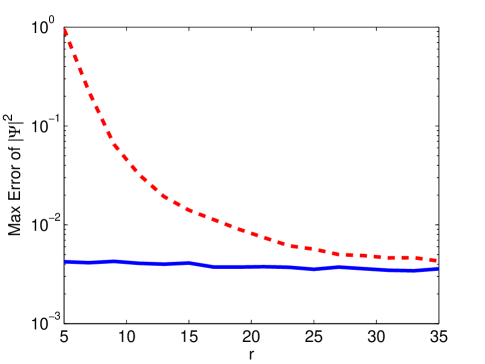
Figure 4: Maximum error of the modulus-squared of a steady-state dark vortex using the L0 (red dashed line) and the MSD (solid blue line) boundary conditions for various domain sizes. The initial numerically optimized solution of the vortex is used as the ‘true solution’ for error comparisons. The simulations were run to an end-time of $t=300$ with a spatial-step of $h=0.25$ and time-step $k=0.01$.

It is clearly seen that a much larger grid is required for the L0 boundary condition to be close to the effectiveness of the MSD boundary condition in this case. For example, it took nearly a $200\times 200$ grid for the L0 boundary condition to produce the same accuracy as the MSD boundary condition did on a $20\times 20$ grid!

As an additional example to test the MSD boundary condition, we simulate two equal-charge vortices whose interaction is known to produce a rotating circular motion of the two vortices orbiting each other [12]. Using a fixed grid size of $171\times 171$, the simulations are run for long times using the L0 and MSD boundary conditions. The results are shown in Fig. 5.

$\begin{array}[]{c}\begin{array}[]{ccc}\includegraphics[width=122.85876pt]{nlse2D_2-vort_h=025_k=001_endt=110001_MOD2_t=0}&\includegraphics[width=122.85876pt]{nlse2D_2-vort_h=025_k=001_endt=110001_MOD2_t=110001}&\includegraphics[width=122.85876pt]{msd2vort10000}\end{array}\\ \begin{array}[]{ccc}\includegraphics[width=137.31255pt]{msd_2vort_l0_xvsy}&\includegraphics[width=137.31255pt]{msd_2vort_l0_xvst}&\includegraphics[width=137.31255pt]{msd_2vort_l0_rvst}\\ \includegraphics[width=137.31255pt]{msd_2vort_msd_xvsy}&\includegraphics[width=137.31255pt]{msd_2vort_msd_xvst}&\includegraphics[width=137.31255pt]{msd_2vort_msd_rvst}\\ \includegraphics[width=137.31255pt]{xvsy10000}&\includegraphics[width=137.31255pt]{xvst10000}&\includegraphics[width=137.31255pt]{rvst10000}\end{array}\\ \end{array}$

Figure 5: Top row, left to right: Modulus-squared of initial condition of two single-charge vortices separated by a distance of $7$ from the center of the grid, snapshot of simulation using L0 boundary condition at time $t=1100$, and snapshot using MSD boundary condition at time $t=10,000$. Second row, left to right: Traced positions of the two vortices (square and circles respectively) over the course of the simulation using L0 boundary conditions, $x$ positions of the two vortices (solid and dashed line respectively) versus time, and the computed radius of one vortex from the center of the grid for an end time of $t=1100$. Third row: Same description as the second row, but using the MSD boundary condition. Bottom row: Same as in the third row, but with an end-time of $t=10,000$ (only times 5000 through 10,000 shown in the $x$ versus $t$ plot). In all simulations the spatial-step is $h=0.25$ and the time-step is $k=0.01$ with a grid size of $171\times 171$.

We see that once again, using the L0 boundary condition causes a break-down in the dynamics, eventually causing the two vortices to decouple from each other and fling into the boundaries. The MSD boundary condition, by contrast, allows for near-perfect rotational dynamics for indefinite simulation times, even for small grid sizes. It is also noticeable that the period of rotation of the vortices is shorter when using the MSD boundary condition when compared to using the L0 boundary condition. Through further simulations with larger grid sizes, we have observed that the period of rotation converges to the same value (between the two values of the period displayed) for both boundary conditions at approximately the same grid-size (around $250\times 250$). Therefore, the MSD boundary condition performs as well as the L0 in terms of rotational period, but much better in terms of long-term dynamics and minimum grid-size requirements.

If the end-time of the simulation is fixed to be such that the vortices will rotate at least one complete rotation (here we use $t=480$), we can record the deviation from perfect circular motion as the grid size (given as the distance, $d$, from the center of the grid to the edge along the $x$ or $y$ direction) is varied. The vortices are tracked during the simulations and the maximum deviation from a constant radius to the center of the rotating vortices is recorded. The results are shown in Fig. 6.

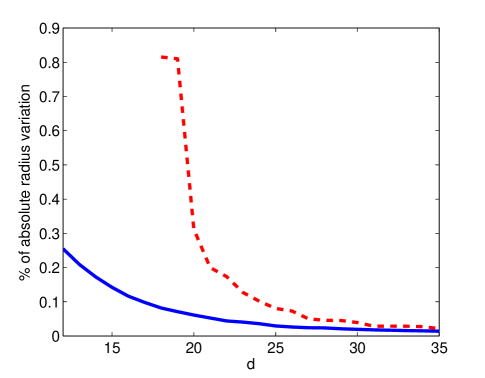
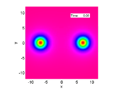
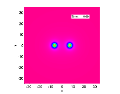
Figure 6: Top: Percentage of absolute radius variation when compared to the initial radius of the vortices to the center of the grid as a function of grid size $d$ (defined as the distance from the center of the grid to its edge along the $x$ or $y$ direction) for a simulation with an end-time of $t=480$ using both the L0 (dashed (red) line) and the MSD (solid (blue) line) boundary conditions. The grid size, $d$, is varied from $12$ (the minimum size required to resolve both vortices adequately) to $35$. Results for the L0 boundary condition below $d=18$ are not shown as the vortices hit the grid wall before the simulation ends. The other simulation parameters are the same as those in Fig. 5. Bottom: Modulus-squared of the initial condition for grid-sizes $d=12$ and $d=35$.

We see that the L0 boundary condition requires a very large grid size to capture the correct dynamics (and completely fails for smaller grids), while the MSD is able to capture the dynamics to an acceptable degree on a much smaller grid-size. The discrepancies when using the MSD boundary condition at low grid sizes (up to $20\%$ radius variation) is understandable since at those distances the boundaries become far from steady-state due to the indentations in the background density due caused by the motion of the vortices.

4.3 Three-Dimensional Dark Vortex Rings in the NLSE

To further show the usefulness of the MSD boundary condition in multi-dimensional settings, we provide one additional example simulation — that of a steady-state vortex ring amidst a co-moving back-flow.

Unlike two-dimensional vortices, vortex rings have an intrinsic transverse velocity associated with them [13]. Therefore, in order to run long simulations of the rings (for instance, to study stability under small perturbations, or interactions between multiple co-moving rings), a very large grid size is required. Often, due to the size of the simulations, a large enough grid is not within the memory limitations of the computers being used for the simulations. To avoid this problem, a vortex ring can be made to be a ‘steady-state’ by applying a background velocity equal and opposite to the vortex ring’s intrinsic velocity. By doing this, long-term simulations of the rings can be performed, but with many fewer grid points.

In Fig. 7 we show a simulation of a moving vortex ring, as well as a steady-state vortex ring amidst a back-flow at various time intervals using the MSD boundary condition. The vortex ring solution is found by seeding the numerically-exact two-dimensional vortex described in Sec. 4.2 (with the correct back-flow velocity added to it) into a nonlinear optimization routine utilizing the two-dimensional axisymmetric version of the three-dimensional NLSE.

$\begin{array}[]{c}\begin{array}[]{ccccc}\includegraphics[width=72.26999pt]{nls3D_1-vrings_h05_t1499707_BC2_M1_P2_MOD2_3DVOL_Frame_2}&\includegraphics[width=72.26999pt]{nls3D_1-vrings_h05_t1499707_BC2_M1_P2_MOD2_3DVOL_Frame_3}&\includegraphics[width=72.26999pt]{nls3D_1-vrings_h05_t1499707_BC2_M1_P2_MOD2_3DVOL_Frame_4}&\includegraphics[width=72.26999pt]{nls3D_1-vrings_h05_t1499707_BC2_M1_P2_MOD2_3DVOL_Frame_5}&\includegraphics[width=72.26999pt]{nls3D_1-vrings_h05_t1499707_BC2_M1_P2_MOD2_3DVOL_Frame_6}\end{array}\\ \includegraphics[width=455.30121pt]{VRSSt0}\\ \includegraphics[width=455.30121pt]{VRSSt1500}\end{array}$

Figure 7: Top row: Snapshots of volumetric inverse renders of the modulus-squared of a vortex ring at equal time intervals from $t=25$ to $t=150$. Middle row: Two-dimensional cuts of the modulus-squared of the initial condition of a steady-state vortex ring amidst a back-flow. Bottom row: Two-dimensional cuts of the same vortex ring at simulation time $t=1500$. All simulations use the MSD boundary condition, spatial-step size $h=0.5$, and time-step $k=0.035$.

The vortex ring remains stationary for very long simulation times (up to $t=1500$ in this case), further demonstrating the MSD boundary condition’s usefulness in studying co-moving solutions. As in the case of the co-moving dark soliton of Sec. 4.1, the MSD boundary condition seems to be the only viable and easy-to-implement boundary condition for simulating a solution containing a co-moving back-flow.

5 Stability

It is well known that boundary conditions can adversely effect the stability of numerical simulations to the point where an otherwise stable scheme can become unstable [1]. Therefore, it is necessary to investigate the stability effects of the MSD boundary condition. However, since the MSD boundary condition is general in nature, its effect on the stability of the simulations will depend on the governing PDE being used, as well as the form of the overall numerical scheme being implemented. Therefore, no general statements about the MSD boundary condition’s stability effects can be made. That being said, in the specific case of the NLSE using the RK4+CD scheme that have we have used for the examples in Sec. 4, the stability effects of the MSD boundary condition can be addressed, the results of which may be useful for a variety of PDEs and numerical methods.

An analysis of the stability effects of using the MSD (and the L0) boundary conditions have been worked out as part of our prior study on the stability of RK4 schemes applied to the NLSE [14]. The relevant results are as follows.

First, in the linear case where $s=0$, and with no external potential ($V({\bf r})=0$), the stability bound on the time-step $k$ of simulating the NLSE utilizing the RK4+CD method, and using standard Dirichlet boundary conditions in a $d$-dimensional setting is given by

$$k_{\mbox{\scriptsize linear}}<\frac{h^{2}}{d\,\sqrt{2}\,a}.$$ (28)

In the general NLSE case, a linearized stability bound is found by treating the nonlinearity $|\Psi|^{2}$ (and the boundary condition terms) as a constant, yielding

$$k<\frac{\sqrt{8}}{\max\{\lVert\vec{B}\rVert_{\infty},\|\forall L_{i},L_{i}-\vec{G}\rVert_{\infty}\}}\,\frac{h^{2}}{a},$$ (29)

where $\vec{B}$ are the boundary points defined as

Bb h2a(s|Ψb|2−Vb)h2aIm[Ψt,b−1Ψb−1],fragments fragmentsB𝑏 fragmentssuperscriptℎ2𝑎(s|Ψ𝑏|2V𝑏)fragmentssuperscriptℎ2𝑎Im[subscriptΨ𝑡𝑏1subscriptΨ𝑏1]\begin{tabular}[]{|l|c|c|c|}\hline\cr$\;$&L0 ($\nabla^{2}\Psi_{b}=0$)&MSD ($|\Psi_{b}|^{2}=\mbox{const}$)\\ \hline\cr$B_{b}$ \rule{0.0pt}{17.22217pt}\rule[-10.76385pt]{0.0pt}{0.0pt}&$\dfrac{h^{2}}{a}\left(s|\Psi_{b}|^{2}-V_{b}\right)$&$\dfrac{h^{2}}{a}\mbox{Im}\left[\dfrac{\Psi_{t,b-1}}{\Psi_{b-1}}\right]$\\ \hline\cr\end{tabular},

L0 (=∇2Ψb0)MSD (=|Ψb|2const)L0 (=∇2Ψb0)MSD (=|Ψb|2const)

the elements of $\vec{L}$ are defined as

$$L_{i}=\frac{h^{2}}{a}\left(s|\Psi_{i}|^{2}-V({\bf r}_{i})\right),$$

and $\vec{G}$ is a set of values determined by the dimension being used, defined as

$$\begin{tabular}[]{|c|c|c|c|}\hline\cr&$d=1$&$d=2$&$d=3$\\ \hline\cr$\vec{G}$&$\{4,3,1,0\}$&$\{8,7,6,2,1,0\}$&$\{12,11,10,9,3,2,1,0\}$\\ \hline\cr\end{tabular}.$$

As mentioned in Ref. [14], since these stability results are based on a linearized approximation to the full nonlinear problem, in practice, one must use a time-step that is slightly lower than the bounds given above. In our experience, setting the time-step to be $80\%$ of the given bounds ensures stability in most cases.

The results show that the MSD boundary condition should not effect the stability greatly, as the $B$ values are $O(h^{2})$, and the value of $\Psi_{t,b-1}/\Psi_{b-1}$ (as discussed in Sec. 2.2) is roughly equal to $i$ times the frequency of the solution at the boundaries, which is typically a reasonable value. Therefore the $L_{i}-\vec{G}$ terms in Eq. (29) will almost always be larger than those in $\vec{B}$, in which case the MSD boundary condition has no effect of the stability requirements. Also, it should be noted that the full stability bound of Eq. (29) is, in practice, often very similar in value to the simple linear bounds of Eq. (28), making the former bound a good practical bound to use.

6 Conclusion

We have shown the formulation of a modulus-squared Dirichlet (MSD) boundary condition for numerical simulations of time-dependent complex partial differential equations. The standard form of the MSD boundary condition is given as a boundary value of the time-derivative of the solution as a function of the solution at that point, as well as the solution and its time-derivative at the closest interior point. It is easily expressed as

$$\left.\frac{\partial\Psi}{\partial t}\right|_{b}\approx i\,\mbox{Im}\left[\frac{1}{\Psi_{b-1}}\left.\frac{\partial\Psi}{\partial t}\right|_{b-1}\right]\,\Psi_{b},$$

where the subscripts $b$ and $b-1$ refer to a boundary point and the closest interior point to the boundary respectively.

Through multidimensional numerical examples of the MSD boundary condition applied to the nonlinear Schrödinger equation, we have shown that it is extremely effective in terms of non-interference with internal dynamics and accuracy, as well as in requiring smaller grid sizes when compared to other boundary conditions currently in use (such as setting the Laplacian to zero at the boundaries). This is especially true in simulations of coherent structures which exhibit vorticity (such as vortices and vortex rings) and in simulations of solutions which have a co-moving background velocity associated with them. In the latter case, the MSD boundary condition seems to be the only simple boundary condition which can handle such co-moving back-flows. We conclude that the MSD boundary condition is as effective as the standard Dirichlet boundary condition for problems with a constant value at the boundary, and nearly as easy to implement.

Appendix A   Sample Implementation of the MSD Boundary Condition

In order to demonstrate the simplicity of implementing implement the MSD boundary condition, we include here the MATLAB implementation of the MSD boundary condition in one-dimension. We assume a time-dependent complex-valued partial differential equation in the form

$$U_{t}=F(U),$$

where $F(U)$ can contain spatial derivatives, nonlinearities, etc. Given a MATLAB function to compute $F(U)$, an initial condition U, storage vector Ut, and using a simple first-order time stepping scheme with time-step $k$, we arrive at the following code:

for(t=0:k:endtime)
    %Store F(U) into a vector.  Here, F(U) sets boundary values to dummy values:
   Ut = F(U);
    %Apply MSD boundary condition to Ut:
   Ut(1)   = 1i*imag(Ut(2)/U(2))*U(1);
   Ut(end) = 1i*imag(Ut(end-1)/U(end-1))*U(end);
    %Take step in scheme:
   U = k*Ut + U;
end

References

- [1] J. C. Strikwerda. Finite Difference Schemes and Partial Differential Equations. Society for Industrial and applied Mathematics, Philadelphia, PA, 2 edition, 2004.
- [2] B. Fornberg. A Practical Guide to Pseudospectral Methods. Cambridge University Press, 1996.
- [3] L. Debnath. Nonlinear Partial Differential Equations for Scientists and Engineers. Birkhauser Boston, New York, New York, 2 edition, 2005.
- [4] B. Malomed. Variational methods in nonlinear fiber-optics and related fields. Progress in Optics, 43 (2002) 71–193.
- [5] P. G. Kevrekidis, D. J. Frantzeskakis and R. Carretero-González. Emergent Nonlinear Phenomena in Bose-Einstein Condensates: Theory and Experiment, volume 45. Springer Series on Atomic, Optical, and Plasma Physics, 2008.
- [6] X. Antoine, A. Arnold, C. Besse, M. Ehrhardt and A. Schädle. A review of transparent and artificial boundary conditions techniques for linear and nonlinear Schrödinger equations. Comm. in Comp. Phys., 4, 4 (2008) 729–796.
- [7] G. H. Golub and J. M. Ortega. Scientific Computing and Differential Equations An Introduction to Numerical Methods. Academic Press, San Diego, California, 2 edition, 1992.
- [8] R. M. Caplan. NLSEmagic: Nonlinear Schrödinger equation multidimensional Matlab-based GPU-accelerated integrators using compact high-order schemes. http://www.nlsemagic.com, (2011).
- [9] C. T. Kelley. Solving Nonlinear Equations with Newton’s Method. SIAM (Fundamentals of Algorithms), 2003.
- [10] D.J. Frantzeskakis R. Carretero-González and P.G. Kevrekidis. Nonlinear waves in Bose-Einstein condensates: physical relevance and mathematical techniques. Nonlinearity, 21 (2008) R139–R202.
- [11] Yuri S. Kivshar, Jason Christou, Vladimir Tikhonenko, Barry Luther-Davies and Len M. Pismen. Dynamics of optical vortex solitons. Optics Communications, 152, 1-3 (1998) 198 – 206.
- [12] D.J. Frantzeskakis P.G. Kevrekidis, R. Carretero-González and I.G. Kevrekidis. Vortices in Bose-Einstein condensates: Some recent developments. Mod. Phys. Lett. B, 18, 30 (2004) 1481–1505.
- [13] P. H. Roberts and J. Grant. Motions in a Bose condensate I. The structure of the large circular vortex. J. Phys. A: Gen. Phys., 4 (1971) 55–72.
- [14] R. M. Caplan and R. Carretero-González. Numerical stability of explicit Runge-Kutta finite-difference schemes for the nonlinear Schrödinger equation. arXiv:1107.4810, (2011).