Resolved Near-Infrared Stellar Populations in Nearby Galaxies

Abstract

We present near-infrared (NIR) color-magnitude diagrams (CMDs) for the resolved stellar populations within 26 fields of 23 nearby galaxies ($\lesssim 4{\rm\,Mpc}$), based on images in the $F110W$ and $F160W$ filters taken with Wide Field Camera 3 (WFC3) on the Hubble Space Telescope (HST). The CMDs are measured in regions spanning a wide range of star formation histories, including both old dormant and young star-forming populations. We match key NIR CMD features with their counterparts in more familiar optical CMDs, and identify the red core Helium burning (RHeB) sequence as a significant contributor to the NIR flux in stellar populations younger than a few $100{\rm\,Myrs}$ old. The strength of this feature suggests that the NIR mass-to-light ratio can vary significantly on short timescales in star forming systems. The NIR luminosity of star forming galaxies is therefore not necessarily proportional to the stellar mass. We note that these individual RHeB stars may also be misidentified as old stellar clusters in images of nearby galaxies. For older stellar populations, we discuss the CMD location of asymptotic giant branch (AGB) stars in the HST filter set, and explore the separation of AGB subpopulations using a combination of optical and NIR colors. We empirically calibrate the magnitude of the NIR tip of the red giant branch (TRGB) in $F160W$ as a function of color, allowing future observations in this widely adopted filter set to be used for distance measurements. We also analyze the properties of the NIR RGB as a function of metallicity, showing a clear trend between NIR RGB color and metallicity. However, based on the current study, it appears unlikely that the slope of the NIR RGB can be used as an effective metallicity indicator in extragalactic systems with comparable data. Finally, we highlight issues with scattered light in the WFC3, which becomes significant for exposures taken close to a bright earth limb.

1. Introduction

Near-infrared (NIR) observations have become increasingly important for studies of galaxies and their evolution over cosmic time (e.g., Conselice et al., 2005; Dahlen et al., 2005; Saracco et al., 2006; Cirasuolo et al., 2010). This trend will no doubt continue during the coming decade, thanks to continued improvements in NIR detectors, the growing maturity of adaptive optics, the installation of WFC3 on HST, and the upcoming launch of the James Webb Space Telescope (JWST).

The importance of NIR observations for galaxy evolution studies rests on the reduced sensitivity of the NIR mass-to-light ratio to dust and to the age or metallicity of the underlying stellar population, particularly compared to the optical or ultraviolet. The NIR luminosity of a galaxy is therefore thought to be a robust indicator of stellar mass (e.g. Thronson & Greenhouse, 1988; Brinchmann & Ellis, 2000; Bundy et al., 2005). However, the ability to correctly interpret NIR observations relies on accurate stellar population modeling, which in turn requires accurate isochrones, stellar lifetimes, and spectra for the evolving stars which dominate the flux at NIR wavelengths (see Conroy & Gunn (2010), for an estimate of current uncertainties).

Recently, there has been some concern that the mass-to-light ratio in the NIR is not nearly as stable as has been assumed. On the theoretical side, Maraston et al. (2006) have suggested that the NIR flux from asymptotic giant branch (AGB) stars may lead to drastically lower mass-to-light ratios when intermediate-age populations are present, as must be the case for in situ observations of young galaxies at high redshift (although see Kriek et al. (2010)). Lower NIR mass-to-light ratios could also help to explain why some elliptical galaxy progenitors at high redshift appear to have stellar densities higher than seen in the local universe (van Dokkum et al., 2008).

The most accurate constraints on evolving stars’ contribution to the NIR come from resolving the stellar populations directly (e.g. Rejkuba et al., 2006; Gullieuszik et al., 2007, 2008; Melbourne et al., 2010a, most recently). With WFC3’s IR channel on HST, we are now able to resolve large numbers of individual stars in nearby galaxies. There are well over a hundred galaxies within the Local Volume ($D\lesssim 4{\rm\,Mpc}$) that are close enough to be targeted for resolved stellar population studies. These galaxies have already been observed extensively with HST in the optical (Dalcanton et al., 2009; Gilbert et al., 2011), and their color-magnitude diagrams have revealed the galaxies to have a wide range of metallicities and star formation histories. These systems therefore form an ideal set for probing the properties of the same stellar populations in the NIR.

To this end, we undertook an HST “snapshot” survey of nearby galaxies with existing high-quality optical data. We took advantage of the high throughput and resolving power of the WFC3 IR channel to produce CMDs of individual fields in 23 galaxies, spanning a variety of stellar populations. In this paper, we present our sample, and characterize the resulting color-magnitude diagrams. These data will be used in subsequent papers to place quantitative constraints on the contribution of AGB and RHeB stars to the total luminosity (Melbourne et al., 2011), on the lifetimes of AGB stars, and on the population of carbon stars.

The outline of the paper is as follows. In Section 2 we present our sample selection, observations, reductions, and matched optical photometry. We also discuss a previously uncharacterized transient scattered light feature in the Wide Field Camera 3 infrared channel (hereafter WFC3/IR). In Section 3 we discuss the origin of different features in the NIR CMDs and optical-NIR color-color diagrams, and highlight the importance of core red Helium-burning (RHeB) stars to the overall luminosity, for populations younger than $\sim 0.5{\rm\,Gyr}$. We discuss the properties of the tip of the red giant branch (TRGB) in the NIR (Section 4), and the AGB and red giant branch (RGB) luminosity function in Section 5. Finally, we discuss the metallicity dependence of the NIR RGB morphology and color on metallicity in Section 6.

2. Data

2.1. Sample Selection

To characterize NIR CMDs as a function of stellar age and metallicity, we require targets whose stellar populations have been constrained using optical observations in tandem with well-calibrated stellar isochrones. We therefore chose SNAP targets from among those nearby galaxies with archival high-quality multi-color imaging (typically from ACS, but in some cases from WFPC2). Of these, we selected a subset of 61 fields in 51 galaxies from the ACS Nearby Galaxy Survey Treasury (ANGST), a volume-limited sample of non-Local Group galaxies out to $\sim\!4{\rm\,Mpc}$ (Dalcanton et al., 2009), and from the archival legacy program ANGRRR: Archival Nearby Galaxies: Reduce, Reuse, Recycle (Gilbert et al., 2011). Based on their HST stellar photometry, we have verified that these target fields have (1) sufficient numbers of stars to contain hundreds of candidate AGB stars within a single WFC3/IR FOV; (2) uncrowded stellar photometry of sufficient quality to provide useful constraints on the star formation history and metallicity distribution; (3) indications from the range of red giant branch colors that the stellar populations host a non-negligible fraction of stars whose metallicities fall outside of the range of well-studied LMC/SMC metallicities; and (4) a sufficiently broad range of star formation histories to allow sampling of evolving stars of different masses. Our target list included multiple pointings in the more massive systems, whenever the optical data suggested that there are significant variations in stellar age and metallicity at different locations within the galaxy.

During Cycle 17 we obtained observations for 26 of the 61 possible SNAP targets. Two galaxies (Holmberg II and NGC 2403) had multiple pointings (2 and 3 pointings, respectively), isolating regions with different star formation histories and metallicities. The properties of the 23 observed galaxies are listed in Table 1. Galaxy names, positions, apparent blue magnitudes ($B_{\rm T}$), diameters, morphological $T$-types, and Hi line widths ($W_{50}$) have been adopted from the primary name in the Karachentsev et al. (2004) Catalog of Neighboring Galaxies. Distance moduli are based on the $F814W$ TRGB from Dalcanton et al. (2009) for most galaxies, and from Karachentsev et al. (2003) for NGC 7793. Group memberships are from Karachentsev (2005) or Tully et al. (2006). Foreground extinctions ($A_{\rm V}$) are from Schlegel et al. (1998), as reported by the on-line Galactic Dust Extinction Service at the Infrared Science Archive.

2.2. Observations

Observations for this program were carried out during Cycle 17 as SNAP-11719. Some fraction of these were taken during the period of instrument commissioning after the Hubble repair mission. All targets were observed in both $F110W$ and $F160W$ with HST’s WFC3 IR channel. These filters offer the greatest depth in a given exposure time, and thus are likely to become the workhorse filters for the WFC3/IR camera. Observations were carried out in a 3-point “WFC3-IR-DITHER-LINE” pattern, with exposures in both $F110W$ and $F160W$ taken at each pointing. We adopted the STEP50 exposure sequence, which accommodates data with a large dynamic range by using both short and long non-destructive reads. We used ${\tt NSAMP}=9$ in $F110W$ and ${\tt NSAMP}=11$ in $F160W$, giving total exposure times of 597.7 s and 897.7 s respectively. The exposure sequence was interleaved to allow buffers to dump during the exposures, with no latency. To maximize the schedulability of our observations, we did not specify a roll-angle orientation constraint.

Properties of the actual observations can be found in Table 2, where we include both the name of the galaxy from Table 1 and the name of the specific target within the galaxy. Target names were chosen to match the names of existing optical data sets at the same position; these associated data sets are also listed in Table 2. The centers of the WFC3 field-of-view (FOVs) were chosen to maximize the overlap with the optical data. The locations of the WFC3/IR footprints are shown in red in Figure 1, superimposed on Digitized Sky Survey images of each galaxy. Blue regions show the locations of the associated optical imaging from ACS or WFPC2. Because we did not specify an orientation, occasionally a small corner of the WFC3/IR FOV fell off the area covered by the optical data. This mismatch occurred in cases where the optical FOV was not centered on the most desirable part of the galaxy, and the scheduled roll angle happened to be unfavorable; however, the fraction of the WFC3/IR FOV lacking optical coverage is less than 10% in almost all cases.

In Figure 4 we show false color images of the observations. There are a number of features to note. First, in many cases it is clear that our short exposures have already reached the “crowding limit”, where stars are sufficiently close on the sky that fainter stars could not be detected, even with longer exposures; this effect can also be seen as spatially-varying depth in the CMDs. Second, background galaxies are far more prevalent than in optical HST images, suggesting that unresolved background galaxies are likely to be a more significant contaminant of the NIR CMDs. Third, the images are marked with a number of circles, located at positions of “IR blobs”, that are flagged as bad data by the WFC3/IR pipeline (see the WFC3-2010-06 ISR by N. Pirzkal). Fourth, extended line emission is visible in $F110W$ images of young star forming regions, as can be seen in the close-up of a star forming region in IC2574-SGS, shown in Figure 17. The line emission in this filter is dominated by the [Siii]9069Å,9532Å doublet, with additional contributions from HeI at 10830Å and 10833Å  (from 2 photon emission) and Paschen $\beta$ at 12818Å.

Finally, and perhaps most concerning, a number of the images show significant scattered light, particularly in the lower left region of the image (see UGC4305-1 or NGC2403-HALO-6, for example). We now discuss the origin of this scattered light component.

2.2.1 Scattered Light

Figure 18 shows the series of 6 combined *FLT images taken during our 1 orbit visit, after all detected sources have been fit and subtracted from the images. The series shows images in both $F110W$ (exposures 1, 3, & 5 in the sequence), and $F160W$ (exposures 2, 4, & 6). The images show two types of structures in the “sky” background. The first is persistent structure due to unresolved stars in the image; this component does not change throughout the visit, but varies from galaxy-to-galaxy. The second structure (falling typically on the left-hand side of the image, and peaking in the bottom left corner), varies rapidly in amplitude during a single orbit but has a consistent shape when present. The pattern of the time variation is not consistent, however, such that the brightness of the scattered light feature peaks at different times during an orbit. This variability leads to an apparent variation of the color of the scattered light; if the scattered light peaks during a $F110W$ exposure, the scattered light can appear blue, but if it peaks during an $F160W$ exposure, the light can appear red.

The rapid variation in the amplitude of the scattered light places strong constraints on its origin, as there are few telescope pointing attributes that vary significantly during an orbit. The angles between the principal V1 axis and the Sun or the moon (FITS header keywords SUNANGLE and MOONANGL) vary little during an orbit, nor does the amount of zodiacal light. The only quantities which do vary on that timescale are the angle between the Sun and the Earth’s limb (keyword SUN_ALT) and, more directly, the angle between the spacecraft pointing and the Earth’s limb (keyword LOS_LIMB in the *.JIT or *.JIF files). We thank Ben Weiner (private communication) for pointing out this possibility, based on his analysis of similar effects seen in WFC3/IR grism data.

To examine the variation of the scattered light as a function of the angle to the Earth’s limb, we analyzed the sky levels in each star-subtracted *.FLT image. We assume that there are three contributors to the star-subtracted “sky” image: (1) a mean uniform background; (2) a spatially-structured, time-invariant background due to unresolved stars; and (3) a spatially-structured, time-variable background due to scattered light, which peaks in the lower left quadrant. To assess these different components, we recorded the mean level in the upper right quadrant of each image, which is assumed to be free of the scattered light feature, and in the lower left region dominated by the feature ([0:308,0:507], in image coordinates). Note that we do not expect these two sky levels to be identical, even in the absence of the scattered light feature, because of the contribution of light from unresolved stars. However, they both should share a common “floor”, representative of the mean sky background during the observation.

In the left hand panel of Figure 19, we show the mean sky level in the upper right quadrant of each exposure, plotted as a function of the limb angle between the spacecraft and the earth, for the $F110W$ and $F160W$ filters, respectively. If the earth’s limb was dark at the time of observation, the sky level is plotted with an open circle. Observations taken within a single orbit are connected with a line.

From the left hand side of Figure 19, it is clear that the sky brightness depends strongly on the limb angle for the $F110W$ filter, at least when the earth’s limb is bright. Below angles of $40{{}^{\circ}}$, the mean sky level increases by roughly a factor of two or more. We expect that this correlation would be significantly tighter if this test were repeated for empty fields, where there would be little contribution from unresolved sources to the measurement of the sky.

In the right hand panel of Figure 19, we attempt to capture the amplitude of the scattered light feature visible in the first two panels of Figure 18. Unfortunately, we cannot simply track the variation of the sky level in that region, since we expect some limb angle dependent variation in the overall sky level, as seen in the left hand plot of Figure 19. Instead, we look at the limb angle dependence of the excess light in the lower left, compared to the upper right (${\rm Gradient}\equiv{\rm Sky}_{lower\,left}-{\rm Sky}_{upper\,right}$). We assume that when the scattered light feature is absent, the difference in the sky level between the upper right and lower left regions reflects the structure in the sky due to unresolved sources. This difference should be constant with time, no matter what the mean sky background level is. For each set of observations (3 per filter in a single orbit), we then look at the “excess” in the difference between the lower left and the upper right, compared to the minimum during the orbit. We then scale the resulting excess by the minimum sky level in the four quadrants of the image, to give an indication of the fractional strength of the feature, compared to the typical sky level when unresolved sources are not present.

The right hand side of Figure 19 shows that for most of the exposures, the relative sky brightness of the lower left and upper right varies by less than 1% between exposures, as long at the angle to the bright earth limb is greater than $30{{}^{\circ}}$. If the angle is less than $30{{}^{\circ}}$, however, a strong scattered light feature is produced in the majority of cases. The onset is quite sharp, and is present in both filters, unlike the increase in the uniform sky brightness with limb angle, which is gradual and much stronger in $F110W$. Based on this analysis, the galaxies with the most prominent scattered light features ($>$4% in either filter) are UGC4305-1, IGC2574-SGS, DDO71, SN-NGC2403-PR, NGC2403-DEEP, NGC2403-HALO-6, and KDG73, in order of strongest to weakest. This ranking agrees with the visual impression seen in the color images in Figure 4.

For our subsequent analysis, we make no additional attempt to compensate for the structure of the scattered light feature in these images. Since our photometry uses a very localized estimate of the sky, our results should be insensitive to this feature, except through having to accept more noise in the affected region. Given the brightness of the stellar sources, including observations with low limb angle observations produces more benefits through increased integration time than are lost through increased noise levels. For many other possible WFC3/IR programs, however, this may not be the case, and observers should consider specifying a minimum earth limb angle for their observations.

There are two additional complications that may result from the presence of rapidly varying scattered light, however. The first complication is that some reads affected by scattered light may have pixels that are erroneously flagged as cosmic rays, if flux in the scattered light feature appears as an outlier compared to the large number of unaffected reads; however, we do not see in any obvious increase in the number of masked cosmic rays in the limb brightened regions in Figure 18. The second complication results from the fact that the final IR image is produced by fitting a linear function to a series of non-destructive reads taken during the course of the exposure. However, while the flux in a pixel from a star will rise linearly during the exposure, the flux from the background will not rise linearly when the angle to the limb or the limb’s brightness changes during an observation. The assumption of a linear fit may therefore be invalid when the flux in the background is comparable to the flux of the source in a given pixel. One should further note that this effect could be present even when the strong scattered light feature is not obvious, since, as one sees in Figure 19, the uniform sky background can vary strongly during the observation, particularly in $F110W$. Unfortunately, it is not straightforward for us to evaluate this effect in our data. First, it is difficult to separate the true time-variable sky background, from the spatially-variable time-constant background from unresolved stars. Second, we cannot use spatial variations in the color magnitude diagram to identify systematic errors in the photometry associated with the scattered light feature, since galaxies typically exhibit significant gradients in the their stellar populations.

2.3. Data Reduction & Photometry

Photometry was performed using the DOLPHOT package (Dolphin, 2000), including a new WFC3-specific module generated in support of this HST program. The core functionality of DOLPHOT remains as in previous versions (i.e., simultaneous PSF fitting across a stack of images aligned to sub-pixel accuracy), but the WFC3 update includes several new capabilities: a preprocessing routine that uses the data quality extensions to mask the image and then applies the appropriate WFC3 pixel area maps, a WFC3 point spread function (PSF) library, WFC3 distortion corrections, and new zero points for WFC3. Pixel area maps, distortion terms, zero points, and encircled energy corrections were obtained from the WFC3 documentation. The PSF library was computed using the preliminary version of Tiny Tim 7.0 with WFC3 support; note that the current version of the WFC3/IR Tiny Tim PSF library is based on pre-flight data. For WFC3/IR, PSFs are computed with 10$\times$10 subsampling and a 3$\arcsec$ radius, for 64 regions on the chip. DOLPHOT also adopts small aperture corrections calculated from uncrowded stars in the image; these corrections were always $\leq$0.01 mag.

All PSF photometry was performed by minimizing residuals on all individual flt exposures, and then combined into final magnitudes for each star in each filter. Non-detections are considered to be stars with signal-to-noise ratios of less than 4, for a given filter. Quality parameters are computed and included in the combined photometry as well. Two catalogs were then produced for each field using the DOLPHOT signal-to-noise, sharpness, and crowding parameters. The first “*.st” catalog contains all sources detected in at least one band with S/N$>$4, where the sharpness of the source does not exclude the possibility that it is stellar (sharpness${}^{2}\,<$0.1). The second “*.gst” catalog only contains the highest quality photometry (including detections with S/N$>$4 in both filters, (sharpness_F110W + sharpness_F160W)${}^{2}\,<$0.12, and crowding_F110W + crowding${}_{F160W}\!<$0.48). The *.gst catalog typically contains $\sim$50$\pm$10% of the sources from the *.st catalog. These final parameter cuts were chosen to produce the cleanest CMD features (few stars outside of the known features) without culling large numbers of sources from the features themselves; the culled sources are almost entirely valid stellar detections, but have more uncertain photometry. The number of stars detected varies between 6,000 and 40,000 per pointing, with a median of $\sim$10,000 (Table 2). We also include the maximum and minimum stellar surface density of the *.st detections, calculated within 100 subregions defined by a 10$\times$10 grid in the image; observations with a higher stellar surface density will be more affected by crowding, and observations with larger differences between the maximum and minimum surface density will have stronger spatial variations in the depth of the CMD and the accuracy of the photometry.

Finally, we assessed the biases in our photometry using artificial star tests. False stars were placed into the image stack 100,000 times, such that the artificial stars sampled the full range of colors, magnitudes, and locations of our real photometry. We recovered the artificial stars using identical photometry routines and post-processing cuts as those applied to the data.

Table 2 includes the resulting “50% completeness” magnitude for each filter, as determined by the limit where 50% of artificial stars inserted into the image are successfully recovered by our photometry (described below) in both filters (as in the *.gst catalog). The 50% completeness limits of our least crowded fields are $\sim$26.2 mag in $F110W$ and $\sim$25.1 mag in $F160W$; these limits were significantly fainter than originally expected for photon-limited sources, based on the pre-flight WFC3/IR Exposure Time Calculator. Note, however, that this depth is frequently position dependent, as can be seen from the position-dependent CMDs in the right hand panels of Figure 4. In crowded regions, the proximity of adjacent stars compromises the recovery of faint stars, producing brighter limiting magnitudes than one would expect based on photon counting statistics alone. The field for SN-NGC2403-PR has been particularly affected by crowding, and has a 50% completeness limit that is more than 2 magnitudes brighter than the median of the sample.

Figure 20 shows the magnitude uncertainties reported by DOLPHOT for the $F110W$ and $F160W$ filters, for the full stellar “*.st” catalog. The small number of points that scatter to larger uncertainties typically come either from regions that were not covered in all three dithered exposures, or that have been flagged as being poorly photometered. The number of stars with higher than average uncertainties are reduced in the culled “*.gst” catalog, which produces somewhat sharper features in the CMD, at the expense of a modest drop in completeness. The effect of this culling can be seen in Figure 21, where we plot the CMDs for the *.st and the *.gst photometry catalogs for one of our fields. We will describe the many features in these CMDs in Section 3 below.

In Figure 22 we show the distribution of $F160W$ magnitude errors for artificial stars inserted into our images, in bins of 1 magnitude, for a crowded and an uncrowded field (left and right plots, respectively). At the extremes, the distributions show a tail towards brighter recovered output magnitudes, due to the blending of faint undetected stars with brighter stars. In the median, however, there is very little bias in the recovered magnitude ($<\!0.02\,{\rm mag}$ in the median for the faintest bin, which is nearly an order of magnitude smaller than the photometric uncertainty at the same magnitude). Recovered colors are even less biased, as crowding typically offsets the magnitudes of both filters in similar directions. The amplitudes of these effects are of comparable amplitude in $F110W$, but are not quite identical due to the different level of crowding and sky brightness in the two filters.

2.4. Matching NIR and Optical Catalogs

We match stellar catalogs from the distortion corrected optical and WFC3 images as follows. We calculate the astrometric transformation by first requiring $\sim$150 stars that are bright in both the optical and NIR data sets, and that spatially span the entire overlap region between the WFC3 and ACS (or WFPC2) images. We produce a list of candidate alignment stars by first culling the optical and NIR star catalogues from DOLPHOT to only stars that are in the spatial overlap region. We then select all reasonably bright, red stars in each dataset (optical color $>\!0.7$ mags and F814W $<\!26$ mags; IR color $F110W-F160W\!>\!0.5$ mags and F160W $<\!24$ mags), producing lists of $\sim$1000 stars in the optical and in the NIR. We sort the resulting two lists by luminosity to preferentially select luminous stars. Rather than selecting the 150 brightest stars, which are frequently spatially clustered and do not span the full chip, we insist that as long as we have more than one star to choose from, we will select stars with an average separation of $\sim 5\arcsec$, ensuring broader areal coverage of the alignment stars.

We derive the transformation between the optical and IR star lists by first visually identifying a roughly linear shift between the two coordinate systems. We then iteratively calculate a final transformation using the “method of triangles” described in Valdes et al. (1995), as implemented in the routine MATCH by Michael Richmond. First we run a linear fit between the two coordinate systems and then we use that solution as a starting point for a quadratic solution. We find that a cubic solution is generally unnecessary for the transformation between the distortion corrected WFC3 and ACS images, but we do use it for the transformation of the two data sets of WFPC2 observations. We apply the transformation to the entire NIR dataset bringing it into the optical coordinate system used for the ANGST and ANGRRR data releases. Note that we make no attempt to tie the images to the global astrometric frame, due to the lack of appropriate astrometric standards in the small WFC3 fields of view.

Once the WFC3/IR catalog has been astrometrically aligned to the optical catalog, we match individual stars in the two catalogs. We consider stars to be a match if the angular separation between the stars is less than $0.07\arcsec$ (i.e., $\sim$0.5 WFC3/IR pixel). Typically 90% of the stars in the NIR catalogue are well matched to a star in the optical catalogue. Unmatched stars typically fall in the ACS chip gap or in the diffraction spikes of optically saturated bright stars.

2.5. Characterizing the Age of the Stellar Population

The morphology of the CMDs that result from our NIR and optical photometry reflect the age and metallicity of the underlying stellar population. To provide an intial constraint of these parameters, we have analyzed the star formation history (SFH) of these galaxies using optical CMD fitting, similar to the procedures described in Williams et al. (2011) and Weisz et al. (2011), but restricted to the optical data that overlap the WFC3/IR FOV.

Specifically, we measured the star formation rate and metallicity as a function of stellar age, by fitting the optical CMDs using the software package MATCH (Dolphin, 2002). We adopted magnitude cuts set to the 50% completeness limits, and then fit the CMDs using linear combinations of the stellar evolution models of Girardi et al. (2002, with updates in , and , ), populated with stars following an IMF with a slope of -2.3 and a binary fraction of 0.35 (with random mass sampling), convolved with the photometric error and completeness statistics derived from artificial star tests. We first fit the data assuming a single foreground reddening and distance, adopting values used in the ANGST survey (Dalcanton et al., 2009) based on the Schlegel et al. (1998) Galactic dust maps and the magnitude of the TRGB, respectively. The best fit provides the relative contribution of stars of each age and metallicity in each field, which is then converted into cumulative stellar mass produced as a function of time. For consistency with Weisz et al. (2011), we restricted the metallicity evolution to be constant or increasing with time, for galaxies in common with the Weisz et al. (2011) dwarf sample. This choice provides more accurate recent star formation histories, at the expense of introducing occasional biases against SF in the oldest bin for the few galaxies with very deep data

To assess the uncertainty of the best fit, we ran extensive Monte Carlo tests. These tests assess two types of uncertainties: (1) random errors due to Poisson sampling of the CMD and errors in photometry; and (2) systematic errors due to deficiencies in the stellar evolution models, or due to offsets in distance, reddening, and/or magnitude zero-points. The Poisson errors are accounted for by generating artificial CMDs from the best-fit convolved model 100 times, and refitting the resulting CMD. While fitting each of these realizations, the systematic errors are assessed by introducing small random shifts in log($T_{\rm{eff}}$) and $M_{\rm{bol}}$. The random values were drawn from a Gaussian distribution with a width of 0.03 in log($T_{\rm{eff}}$) and 0.41 in $M_{\rm{bol}}$. The size of these shifts are set by differences between models in the literature, and therefore serve as a proxy of the effects of our particular choice of stellar evolution models. Our final uncertainties are the 68% confidence intervals of the results of all of our Monte Carlo test fits. These total uncertainties are used as the error bars in all subsequent plots and analysis. Note however that adjacent time bins in the SFH are covariant to some degree, such that when one time bin fluctuates high, the adjacent bins fluctuate low. As a result, the plots of the cumulative SFH offer a truer representation of the uncertainties.

The resulting SFH and cumulative age distributions are shown in the bottom panels of Figure 23. The lower left panel shows the SFR as a function of time, and the lower right hand panel shows the cumulative star formation history, measured from the present back to $14{\rm\,Gyr}$ ago. A detailed discussion of the SFH analysis of the NIR CMDs will be discussed in an upcoming paper.

3. Color Magnitude Diagrams

In this section we describe the properties of stellar populations in the $F110W\!+\!F160W$ filter set using both models (Section 3.1) and observations (Section 3.2). We discuss the qualitative dependence of these properties on the age of the stellar population, as derived from optical CMDs in Section 2.5.

3.1. Overview of Key Features in Model CMDs

To elucidate interpretation of the CMDs, in Figure 49 we show simulated NIR color magnitude diagrams, color-coded either by age or stellar mass (for a constant star formation rate at a fixed metallicity of [Fe/H]=-1.45), or by metallicity (for a burst of star formation between $8.9$ and $11.2{\rm\,Gyr}$). These simulations include the updated models for AGB mass-loss at low metallicity described in Girardi et al. (2010), and use the artifical stars from the M81-DEEP field to calculate typical photometric uncertainties and biases. Comparable figures for optical CMDs can be found in Dalcanton et al. (2009).

In both the optical and the NIR, the most prominent feature is the red giant branch (RGB), found at colors of $F110W\!-\!F160W\!\sim\!0.8$ in the NIR and $F606W\!-\!F814W\!\sim\!1$ or $F475W\!-\!F814W\!\sim\!2$ in the optical. This color depends on metallicity (Section 6), and becomes bluer when the metallicity is low (Aaronson et al., 1978). At low metallicities, the optical RGB also becomes more vertical and exhibits less curvature. In the NIR, however, the slope of the RGB is nearly vertical, with only modest variations with metallicity (Ferraro et al., 2000). The ages of stars in the RGB can span a wide range ($\gtrsim\!1{\rm\,Gyr}$). For the galaxies in our sample, early star formation is particularly vigorous (Weisz et al., 2011; Williams et al., 2011), which will weight the population of RGB stars towards older ages, compared to the constant SFR shown in Figure 49.

One of the most prominent features along the RGB is the “red clump”, typically found at 3-4 magnitudes fainter than the TRGB in the optical. The stars in the red clump are burning Helium in their cores in the same way as horizontal branch stars, but appear red due to either their young ages (large envelope mass) or their high metallicities (see Girardi & Salaris (2001); Salaris (2002); Castellani et al. (2000) for theoretical models and Ivanov & Borissova (2002); Grocholski & Sarajedini (2002); Valenti et al. (2004) for observational constraints from globular clusters). Unfortunately, our NIR data does not reach this information-rich feature, due to the shortness of our NIR exposures and the bright crowding limit resulting from the larger WFC3/IR pixel scale. The absence of this feature reduces the utility of using our NIR CMDs to constrain the relative amounts of ancient and intermediate age SF.

Ancient star formation also produces a population of low mass thermally pulsing AGB stars (TP-AGB; $<1.5{\rm\,M_{\odot}}$), found just above the TRGB at $M_{\rm{F814W}}\!\sim\!-4$. At younger ages, TP-AGB stars are more massive and have much brighter magnitudes (Marigo et al., 2008). As we discuss below in Section  3.2.1, the colors of AGB stars vary little in the NIR, and thus produce nearly vertical sequences for all but the smaller population of red extreme AGB stars (e.g. Nikolaev & Weinberg, 2000; Gullieuszik et al., 2008; Melbourne et al., 2010a; Davidge, 2010).

Figure 49 shows that younger stars are expected to dominate the stellar populations blueward and brightward of the RGB. The youngest stars are main sequence stars, found at the bluest edge of the CMD. While the main sequence is quite well defined in the optical, it is not nearly as distinct in the NIR. This difference must result in part from the fact that only the most luminous high mass main sequence stars are detectable in these NIR observations. In the optical CMDs, we typically detect main sequence stars with masses of $4.5{\rm\,M_{\odot}}$ and above, whereas in the NIR, we can typically only detect main sequence stars with $\gtrsim 20{\rm\,M_{\odot}}$ (assuming a magnitude limit of 25 mag in $F160W$ versus 28 mag in $F814W$, for a median distance of $3.5{\rm\,Mpc}$ and metallicity of $0.1Z_{\odot}$). Such stars are typically rare, and thus the detectable main sequence will not be sufficiently well-populated to appear as a distinct sequence unless there has been ample very recent star formation.

Complicating the clear detection of the main sequence in some cases is the presence of slightly older blue helium core burning (BHeB) stars. These are evolving post-main sequence $5\!-\!20{\rm\,M_{\odot}}$ stars, with ages of typically $10-500{\rm\,Myr}$. These stars, along with their red counterparts (RHeB stars), are formed following the exhaustion of core hydrogen burning, when the core rapidly collapses and the stars’ effective temperature decreases. The core soon reaches an equilibrium, when core helium burning and inner shell hydrogen burning commence, expanding the redder outer layers. A star at this phase is known as a red helium burning star. As helium in the core is converted into carbon, the RHeBs become visibly hotter and enter the blue helium burning (BHeB) phase of evolution (e.g., Langer & Maeder, 1995). Although the BHeB phase occupies a large fraction of the total core helium burning lifetime (e.g., Bertelli et al., 1994), stars are capable of alternating between BHeB and RHeB stages, with the precise lifetimes determined by the intricate relationships between underlying physical parameters (e.g., Chiosi et al., 1992).

The red and blue core helium burning sequences are most obvious at optical wavelengths. They appear as two sequences emerging brightward of the red clump, where low mass $\lesssim 2{\rm\,M_{\odot}}$ core helium burning stars are found. The BHeB sequence emerges diagonally, heads to bluer colors at higher luminosities, then becomes vertical and parallel to the main sequence at high luminosities and high stellar masses The RHeB sequence emerges nearly vertically from the red clump, and extends steadily brightwards, at somewhat bluer optical colors than the RGB. Along these sequences, stars of a given mass appear at a single luminosity, so that the number of stars along the sequences indicate the numbers of evolving stars of different masses. This connection allows the star formation rate between $\sim$5 and $\sim$400 Myr to be essentially read off the sequence, as was pioneered by Dohm-Palmer et al. (2002), and more recently discussed in McQuinn et al. (2011). More massive, and thus younger, stars appear at very bright magnitudes along both the BHeB and RHeB sequences. However, we note that the models for these stars are currently uncertain, and are known not to produce the correct colors or relative number of stars on the red and blue sequences at low metallicities (Dohm-Palmer & Skillman, 2002; McQuinn et al., 2011).

3.2. Observed Properties of NIR CMDs

We now turn to the observed NIR and optical CMDs for the fields covered by our WFC3/IR observations, shown in the top panels of Figure 23. In the upper left panel of Figure 23, we show the NIR CMD of the cleaned *.gst photometry catalogs, uncorrected for foreground extinction or reddening. In the adjacent panel, we show the highest quality optical CMD that is available from overlapping archival imaging. The stars in the optical CMD have been restricted to those that overlap the area covered by the WFC3/IR FOV. These observed CMDs can be compared with the models in Figure 49 to understand which phases of stellar evolution are populating various features in the CMD. We now discuss the principal features of these CMDs.

3.2.1 Old and Intermediate Age Populations: The AGB & RGB

In a broad qualitative sense, the NIR CMDs in Figure 23 show the features expected from the stellar models, particularly at old ages. In fields dominated by old stellar populations (as judged from the optical CMD; see KDG 63, or NGC 404 for examples), the NIR CMDs are quite simple. They show roughly 3 magnitudes of a well-defined upper red giant branch terminating at $M_{\rm{F160W}}\!\sim\!-5.7$. The red giant branch is more vertical and exhibits less curvature than in the optical (see M81-DEEP for an example), as expected from Figure 49. The color at the tip of the RGB varies from between 0.7 and 1.1, as we discuss in more detail in Section 4 below. This range of colors agrees well with the range expected from the models in Figure 49. Unfortunately, the data are not deep enough to reveal the red clump in the NIR; this feature is expected to appear $\sim\!4$ mag below the TRGB.

Galaxies dominated by old stars also host a sparse population of TP-AGB stars located above the tip of the RGB ($M_{\rm{F160W}}\!\lesssim\!-5.7$). The NIR population of TP-AGB stars falls in a vertical sequence spanning a narrow range of color, in contrast to the broad “fan” of TP-AGB stars seen in the optical. At optical wavelengths, the TP-AGB stars span a wide range of colors, due to a combination of dust in their circumstellar envelopes, large variations in molecular line spectra with photospheric temperature, the distance between the optical and the NIR peak of an AGB’s star bolometric flux (Frogel et al., 1990), and long-period variability (which affects all passbands, but only produces significant color spreads in the optical).

The NIR TP-AGB sequence typically extends $\lesssim$1 magnitude in $F160W$ above the TRGB. However, the TP-AGB reaches even brighter magnitudes in populations with more recent intermediate age SF (see NGC 3741, for an example). The existence of bright, massive TP-AGB stars at younger stellar ages is predicted by the models as well (see Figure 49, and luminosity functions in Olsen et al. (2006)).

At lower luminosities in the TP-AGB sequence, CMDs sometimes show a noticeable “gap” between the brightest RGB stars and the faintest TP-AGB stars above the TRGB (see NGC2403-HALO-6). This localized drop in the luminosity function seems to have a counterpart in evolutionary tracks of TP-AGB stars (Marigo & Girardi, 2007). The minimum likely reflects the steeper rate of brightening ($-dM_{\rm{bol}}/dt$) that characterises the initial stages of the TP-AGB phase, when the first thermal pulses have still not reached the full-amplitude regime and TP-AGB stars are expected to be fainter than predicted by the core mass-luminosity relation. As a result, the brighter late stages of TP-AGB evolution are slower, such that luminosity bins appear relatively more populated than the fainter early stages. Simulated CMDs based on the Marigo & Girardi (2007) TP-AGB models do show a local minimum in the luminosity function right above the TRGB, as expected. However, the gap is not apparent in the more recent models described in Girardi et al. (2010) (lower right panel of Figure 49). The observation of this features opens the possibility that it could help to calibrate the models at the early stages of the TP-AGB.

The mean color at the base of the TP-AGB sequence is comparable to the mean color at the tip of the RGB, such that the TP-AGB sequence appears to emerge vertically from the RGB. However, the cumulative distributions of colors immediately above and below the TRGB suggests that the AGB is slightly redder by 0.02-0.04 magnitudes for galaxies where there is minimal contamination from RHeB stars (e.g., KKH37, HS117, DDO82, DDO78, N2976). Visually, the TP-AGB sequence appears to span a smaller range of color than the RGB in some cases. However, there is no statistical evidence that this is the case, as both the RGB and TP-AGB have statistically indistiguishible widths, when the fewer number of stars in the AGB is taken into account.

We note that our sample does not immediately show a large obvious population of carbon-rich AGB stars. In the corresponding $J+H$ ground-based NIR filter set, such stars dominate a roughly diagonal sequence that starts near $M_{\rm{H}}\!\sim\!-7$ and extends to redder colors and fainter magnitudes. To illustrate this sequence, we show empirical data in Figure 50, using $J-H$ vs $H$ CMD for 2MASS observations of the the LMC. This filter combination is the closest match to the $F110W\!+\!F160W$ filter set used in our observations. In the LMC data the sequence of carbon-rich and/or extreme AGB stars is roughly horizontal at $M_{\rm{H}}\sim-7.3$, and extends redward from the sequence of more numerous oxygen-rich AGB stars. There are a few cases where a comparable red sequence of extreme AGB stars is hinted at in our data (e.g., UGC4305, NGC4163, NGC2403-HALO-6, NGC0300-WIDE1, DDO82). However, in none of these is the sequence as noticeable as in the LMC.

The absence of a strong carbon star tail is initially suprising given that our sample of galaxies is dominated by lower metallicity galaxies than the LMC. The dredge-up of carbon is believed to be more efficient at lower metallicities, both because of more favourable conditions for the occurence of strong helium shell flashes (Karakas et al., 2002; Stancliffe, 2006), and because of the lesser carbon dredge-up needed to reach a carbon-rich condition (with C/O$>$1 at the surface). Thus, one expects carbon-rich stars to be more numerous in low metallicity galaxies. Empirically, this trend has been seen in several studies (e.g., Battinelli & Demers, 2005; Groenewegen, 1999, 2007; Boyer et al., 2011).

On the other hand, carbon-rich stars of low metallicity are significantly hotter than at solar metallicities, which inhibits the formation of the molecules that cause the spectral features typical of carbon stars (Marigo & Girardi, 2007). The resulting reduced opacity in low metallicity carbon-rich stars (e.g., Marigo & Aringer, 2009) may move the carbon stars back to bluer NIR colors than their high metallicity counterparts (see, for instance, Figure 7 of Marigo & Girardi, 2007). Thus, while carbon stars may be more numerous in low metallicity systems, they may be less obvious outliers in NIR CMDs. The difficulty of identifying carbon stars in the NIR has been demonstrated empirically by Battinelli & Demers (2009) for galaxies within the Local Group.

We believe that the lack of obvious carbon stars is further exacerbted by use of the $F110W$+$F160W$ filter set. Simulations with TRILEGAL (Girardi et al., 2005; Girardi & Marigo, 2007) shown in Figure 51 indicate that the majority of carbon-rich AGB stars occupy similar locations as oxygen-rich AGB stars in the WFC3/IR CMDs. These simulations were performed using both the Loidl et al. (2001) (top row) and Aringer et al. (2009) (bottom row) synthetic spectra for C stars. Whereas carbon stars are distinctly redder in $J-H$ than the oxygen-rich AGB (left column), in $F110W-F160W$ they are (if anything) slightly bluer (middle column), particularly for the Aringer et al. (2009) atmosphere models. The properties of the carbon-rich AGB population in our sample will be explored in more detail in an upcoming paper.

3.2.2 Young populations: The Importance of Red Core Helium Burning Stars

In contrast to older stellar populations, young stellar populations have surprisingly complex NIR CMDs. Fields with the most active star formation show far more features than just the RGB and AGB (see targets IC2574-SGS (in I2574), NGC0300-WIDE1 (in N300), UGC4305-1 (in HoII), and UGC5139 (in HoI)). We now identify and briefly discuss these various features.

Star forming NIR CMDs host a vertical sequence at $F110W-F160W\!\sim\!0$ on the blue side of the CMD, made up of both main sequence and BHeB stars. They also show a broad cloud of stars with colors intermediate between the main sequence and the RGB. These stars are most likely to be BHeB stars and other evolving massive stars. Note that only the most massive blue stars are detectable in the NIR. Such stars are rare, making it less likely that a “sequence” will be sufficiently well-populated to appear as a distinct feature (see Figure 49), which reduces the clarity of the main sequence. In fields with on-going but low intensity star formation (e.g., targets NGC3741, NGC7793-HALO-6, NGC3077-PHOENIX), the “main sequence” manifests more as a blue edge to the cloud of points, rather than the narrow sequence seen in the optical.

To elucidate the correspondence between features in the optical and NIR CMDs, in Figure 52 we show CMDs for stars that have been matched between the NIR and optical photometry catalogs (§2.4) for IC2574-SGS, after correcting for foreground extinction and distance. The stars have been color-coded by their likely evolutionary phase, as deduced from the optical. For this exercise, we use optical catalogs involving the $F555$ filter, which provides good separation of CMD features, particularly between main sequence and BHeB stars, and between RHeB and RGB stars. Stars that did not have high quality positional matches (coincident within 0.07$\arcsec$), or that were faint in $F814W$, are plotted in black. We note that the matching is unlikely to be perfect, and that some modest fraction of stars in the NIR catalog may have been incorrectly matched with stars in the optical catalog. This mismatching would be most likely in the crowded star-forming regions in this particular field, where slight errors in the alignment could still leave stars within the error radius for matching.

Figure 52 reveals a number of features. First, as expected, the main sequence stars (in blue) crowd along the blue edge of the NIR CMD. However, the blue core helium burning stars (in green) also contribute the blue vertical sequence, as well as filling the region between the NIR vertical blue sequence and the RGB. Thus, the lack of a clear BHeB sequence in the NIR is due primarily to its merging with the MS. On the red side of the NIR CMD, we see the RGB (red) and AGB (cyan) features discussed in §3.2.1, along with a modest horizontal tail of likely carbon-rich AGB stars at $M_{\rm{F160W}}\!\sim\!-7$. In addition to the AGB stars seen in the CMDs of older stellar populations there is a brighter plume of AGB stars extending brightward of $M_{\rm{F160W}}\!\sim\!-7.5$ and $M_{\rm{F814W}}\!\sim\!-5$. This plume is likely due to the presence of more massive stars on the AGB, as a result of the strong SF at $t<2{\rm\,Gyr}$ in the IC2574-SGS field. Note also that the AGB stars fall on a well-defined sequence in the NIR CMD, but spread over a wide swath of color in the optical, as discussed above in Section 3.2.1.

The most remarkable feature in Figure 52 is the strong sequence of luminous RHeB stars. The color of the sequence is only slightly bluer than the AGB and RGB (by $\sim\!0.2$ mag), and extends to far brighter magnitudes. Indeed, the red core Helium burning evolutionary phase is responsible for all of the most NIR luminous stars in IC2574. As can be seen in Figure 17, these luminous RHeB stars are tightly clustered within an active star forming region that features several young clusters spanning a $\sim\!100{\rm\,Myr}$ range of ages. Looking at the optical image (left), the youngest clusters in the region ($\lesssim 10{\rm\,Myr}$) are still embedded in luminous HII regions, while the slightly older clusters are somewhat fainter, more diffuse, and lack extended line emission, although they are still quite blue, due to large concentrations of luminous BHeB stars. However, in the NIR (right), the relative luminosities of these clusters are reversed, such that the youngest clusters have negligible NIR emission, but the slightly older clusters have large concentrations of extremely luminous RHeB stars.

Thus, although much recent work has focused on the importance of the AGB phase to setting the NIR colors and luminosities of young stellar populations (Maraston et al., 2006; Henriques et al., 2010), it appears that RHeB stars can potentially be equally important. We demonstrate this in Figure 53, where we show the integrated luminosity of stars in different evolutionary phases. At the limit where our data becomes incomplete, RHeB stars are the dominant contribution, followed by AGB stars. The RGB, which is canonically assumed to dominate the NIR light, is only the third most important contributor to the luminosity at the completeness limit of our data. Note, however, that the fractional contribution of RGB stars will increase when the full range of stellar luminosities is considered; corrections for the missing stars are included in a companion paper by Melbourne et al. (2011), where the fraction of integrated light contributed by RHeB and AGB stars is quantified, showing that the RHeB can contribute up to 25% of the total light in $F160W$, and that current models underpredict the luminosity contribution of RHeB stars by up to a factor of 4.

The contribution of RHeB stars to the total luminosity will be strongest when the SFR has been elevated between 25 and $\sim\!100{\rm\,Myrs}$ ago, which produces RHeB stars brighter than $M_{\rm{F814W}}\!\sim\!-5$. This timescale is the same as the one over which UV emission is expected to be significant, and thus surveys that select for galaxies with high UV flux may also be selecting for galaxies with a significant RHeB population. Failure to account for the luminous, somewhat blue RHeB population would lead one to overestimate the mass-to-light ratio in the NIR, and to infer lower metallicities from the broad-band colors. Unfortunately, the models of RHeB stars are even more uncertain than for AGB stars, and are known to produce erroneous colors and relative numbers of BHeB and RHeB at some metallicities (Langer & Maeder, 1995; Dohm-Palmer & Skillman, 2002; Gallart et al., 2005; McQuinn et al., 2011)

Our conclusions about the importance of RHeB stars are not significantly affected by uncertainties from foreground contamination. Unlike studies in the Magellanic Clouds, our fields cover small areas on the sky, which minimizes contributions from bright Milky Way stars. The lack of luminous contaminants can be seen empirically in Figure 4 (presented below), where we show the CMD of different subregions in the chip. We see essentially no luminous stars in the outer regions of small galaxies, where we are presumedly dominated by foreground stars and background galaxies (see HS117, for example). Predictions from the default TRILEGAL Milky Way model (Girardi et al., 2005) also suggest that we expect fewer than one contaminating star in each of the NIR CMDs plotted in Figure 23.

We also note that individual RHeB stars could easily be confused as individual stellar clusters, in images of galaxies that are nearby, but that are not sufficiently close to resolve individual stars. Due to their high luminosity and red colors, it may be difficult to distinguish single IR-luminous RHeB stars from older stellar clusters with larger numbers of fainter RHeB stars.

3.3. Color-Color Diagrams

We can further explore the separation of different stellar evolutionary phases using the optical-NIR color-color diagram. We adopt the target IC1574-SGS as a test case, and use the matched catalogs from Figure 52 to generate an optical-NIR color-color diagram, color-coded as in Figure 52. The resulting color-color diagram is shown in Figure 54.

Figure 54 shows that the optical and NIR colors are highly correlated for colors bluer than $F555W-F814W\!\lesssim 1.7$. In this regime, the optical and NIR colors track each other extremely well, and are thus of little utility for separating phases of stellar evolution in data of this quality. At redder colors, however, there is noticably decreased correlation between the optical and NIR colors, driven almost entirely by the behavior of the AGB population (cyan points in Figure 54). Although the bluest AGB stars follow a narrow sequence of optical-NIR colors, the optically redder AGB stars are far less well-behaved. To first order, the NIR color saturates at $F110W-F160W\!\sim\!1$ for a wide range of optical colors, with the exception of a likely population of extreme AGB stars (Blum et al., 2006). Qualitatively, it appears that the narrower blue AGB sequence bends over to fixed NIR color with increasing optical color. Beyond $F555W-F814W\!\gtrsim\!1.7$, the narrow sequence appears to become embedded in a larger swath of red AGB stars, for which there is little correlation between optical and NIR color, and wide dispersion. There is no qualitative evidence for the narrower sequence continuing redwards of $F555W-F814W\!\gtrsim\!2.2$.

We can further explore these different regimes of AGB behavior by qualitatively separating the AGB sequence into two regions and examining the behavior of the stars in the NIR CMD. Figure 55 shows the adopted division of the AGB population in color-color space (upper left), and the resulting NIR CMD (upper right). Although the division into two classes is somewhat arbitrary, and not motivated by a particular choice of stellar model, the adopted separation does appear to break the AGB population into two luminosity classes. As shown in the histograms in the lower left panels, the redder, high-dispersion sub-population is a constant fraction of the AGB stars brighter than $M_{\rm{F160W}}\!<\!-6.8$, it also lacks lower luminosity AGB stars, and makes up fewer than 10% of the stars fainter than $M_{\rm{F160W}}\!>\!-6.2$. In light of our selection criteria, this luminosity difference suggests that the higher luminosity, more massive AGB stars have systematically redder optical colors (lower right panel) and/or bluer NIR colors (with the exception of the extreme AGB stars redward of $F110W-F160W\!\gtrsim\!1$). Brighter than $M_{\rm{F160W}}\!<\!-6.8$, however, we see no noticible difference in the NIR luminosities or median NIR colors of the two sub-populations (beyond the larger dispersion in the NIR color expected by the adopted division of the two populations in color-color space).

Although Figure 55 suggests that there are systematic luminosity-dependent differences in the optical-NIR colors of AGB stars, we currently lack a physical model that would allow us to make better motivated choices for dividing the AGB population on the basis of optical-NIR colors. It is tempting to think that the division we have made is helping to isolate carbon stars, based on the behavior seen in Figure 51. On the other hand, that same figure shows the large current uncertainties in the modeling at the relevant wavelengths. A more definitive approach to isolating and modeling carbon stars will likely require observations at somewhat longer wavelengths than are currently possible with WFC3’s IR channel, or the addition of narrow-band imaging.

3.4. Spatial variations

In addition to the field-to-field variations of the NIR CMDs discussed above, we also find strong spatial variations within individual fields. Such variation is naturally expected if young and intermediate age populations contribute significantly to the NIR CMD. In the right hand panels of Figure 4 we show the NIR CMDs in 16 subfields within each WFC3/IR frame, next to a color image of the same frame.

These grids show a number of features. First, one can see the effects of crowding. In the most well-populated fields, the depth of the CMD is strongly dependent on position, such that the densest subregions have the shallowest depth. Second, one can see significant spatial variations in the underlying stellar populations, particularly in fields that have significant amounts of recent star formation. Features due to the main sequence, RHeB, and AGB vary in strength and luminosity within individual fields. As an example, in NGC0300-WIDE1 the stellar populations from the left side of the frame host a prominent main sequence and luminous RHeB stars, whereas these populations are nearly absent from the lower right of the frame. Finally, CMD features due to young stellar populations typically appear with more clarity in the subregions than in the field as a whole (for example, note the sharp localization of the RHeB and BHeB in the upper left quadrants of IC2754-SGS, or in the relative population of the AGB and RGB across the field).

4. Tip of the Red Giant Branch in the NIR

In the optical, the magnitude of the tip of the red giant branch has become a widely used distance indicator for galaxies with resolved stellar populations (Lee et al., 1993; Sakai et al., 1996; Méndez et al., 2002; Karachentsev et al., 2006; Makarov et al., 2006). Its utility as a distance indicator rests on the relative insensitivity of the TRGB magnitude to age (for age$\gtrsim\!3{\rm\,Gyr}$) or metallicity (for [Fe/H]$\lesssim\!-0.5$) in the $I$ band, where the bolometric magnitude of RGB stars typically peak (Lee et al., 1993).

In the NIR, however, the behavior of the TRGB magnitude is quite different. Theoretical models indicate that the magnitude of the TRGB should vary significantly with the properties of the underlying stellar population (Figure 2 of Salaris & Girardi, 2005), complicating the use of the NIR TRGB as a distance indicator. The variation in the NIR TRGB magnitude is known to be metallicity-dependent for sub-solar metallicities ($\lesssim 0.5Z_{\odot}$), as has been demonstrated conclusively in data for globular clusters in the 2MASS filter set (Valenti et al., 2004). One can therefore potentially correct for the $\lesssim 1$ magnitude variation in the NIR TRGB absolute magnitude if the metallicity is known, allowing the TRGB to be used as a distance indicator in the NIR.

Unfortunately, this basic approach may not be effective in extragalactic systems, where the mean metallicity is uncertain, and the underlying stellar population is more complex. As shown in Figure 10 of Melbourne et al. (2010b), the presence of intermediate age stars ($1-2.5{\rm\,Gyr}$) shifts the NIR TRGB to significantly fainter magnitudes. However, one could potentially diagnose the presence of this population through other means (for example, through a larger population of bright AGB stars), and correct for it. The metallicity dependence could likewise be corrected for as well; since metallicity directly affects the color of the RGB, it should be possible to empirically calibrate a relationship between the magnitude and color of the TRGB.

In this section, we derive the magnitude and color of the TRGB for our sample. We assume that the distances in Table 1 (based on $F814W$ TRGB measurements) are correct, and then derive the absolute magnitude of the NIR TRGB. In what follows, all magnitudes and colors have been corrected for the foreground extinction given in Table 1, assuming that $A_{\rm{F110W}}/A_{\rm{V}}=0.33669$ and $A_{\rm{F160W}}/A_{\rm{V}}=0.20443$ (Girardi et al., 2008, , updated to included the latest in-flight calibrations for the WFC3 filter sets).

As a first step, in Figure 56 we plot the observed luminosity functions of the red extinction-corrected stars (dark black histogram), and their median color in magnitude bins (red line, plotted only for bins with more than 12 stars). Red stars are selected using a magnitude-dependent color cut to suppress the contribution of bluer young BHeB and MS stars; brighter than the TRGB, we keep all stars redward of $F110W-F160W=0.5$, and fainter than the TRGB, we keep all stars redward of the diagonal line connecting $m=m_{\rm{TRGB}}$, $F110W-F160W=0.5$ with $m=m_{\rm{TRGB}}+4$, $F110W-F160W=-0.2$. This cut has no appreciable effect on any feature visible in the luminosity function. The luminosity functions have not been corrected for incompleteness, and we therefore expect them to roll over at faint magnitudes due solely to observational effects; we carry out a full correction for these effects in Melbourne et al. (2011), where we analyze the NIR luminosity contributed by different evolutionary phases.

Figure 56 shows that there is a clear variation in the absolute magnitude of the TRGB, relative to a fiducial TRGB absolute magnitude of $M_{\rm{F160W}}=-5.7$, plotted as a vertical dotted line. Visual inspection shows that redder RGBs typically terminate at brighter absolute magnitudes; for these presumably metal rich RGB stars, the bolometric flux peaks at redder wavelengths, increasing the flux in the NIR. In some cases one can also see the slight dip in the number of stars just brightward of the TRGB that was discussed in Section 3.2.1 (for example, see UGC4459, NGC4163, NGC3741, NGC2976-DEEP, and IC2574-SGS for particularly obvious cases).

To quantify the variation in the TRGB, we measure the TRGB magnitude in $F160W$ using the edge-detection filter described in Méndez et al. (2002) applied to a Gaussian-smoothed luminosity function as in Sakai et al. (1996) and Seth et al. (2005). Although more sophisticated techniques exist (e.g., Makarov et al., 2006; Frayn & Gilmore, 2003), the TRGB of our sample is typically well-populated and falls well above the photometric limit of the data, making our use of the widely used and calibrated edge-detection technique adequate for an initial distance measurement. We use the identical procedure as was used to measure the TRGB for the optical data (Dalcanton et al., 2009), making the $F814W$ and NIR TRGB directly comparable. Specifically, after extinction correcting all magnitudes and colors, we restrict our analysis to stars on the RGB by iteratively fitting a line to stars that are less than 1 magnitude fainter than the estimated TRGB and that have colors consistent with potential RGB stars ($0.6<F110W-F160W<1.1$). We retain all stars that are within $2\sigma$ of the fit to the RGB sequence towards the red, and within $1.5\sigma$ to the blue; we use the more restrictive cut towards the blue to suppress the contribution from RHeB stars. The candidate RGB stars were then used to construct a Gaussian-smoothed luminosity function, which was then passed through an edge-detection filter.

The final TRGB magnitude and uncertainty was measured by executing 750 Monte Carlo bootstrap resampling trials. In each trial, additional Gaussian random errors were added to the stars’ photometry, based on the magnitude of each star’s photometric error. The TRGB for each trial was taken to be the magnitude corresponding to the peak of the edge-detection response filter within a 1 magnitude interval around the likely TRGB. We then fit the histogram of the returned TRGB magnitudes with a Gaussian at $m_{\rm{TRGB}}$, taking the mean and width of the Gaussian to be the magnitude of the TRGB and its uncertainty. These quantities are converted to absolute magnitudes using the distance moduli in Table 1, adopted from the TRGB analysis in $F814W$.

Once the magnitude of the TRGB has been measured, we characterize the color of the TRGB using stars within 0.05 magnitudes fainter than the TRGB; in the few cases where there are fewer than 15 stars within the adopted magnitude range, we increase the range to 0.1 magnitudes. We calculate the mean and standard deviation of these stars’ colors using a biweight, iteratively clipping stars within 2$\sigma$ of the biweight mean, which visual inspection suggests captures all the width of the TRGB with acceptable rejection of RHeB stars.

Figure 59 shows the resulting absolute TRGB magnitude in $F160W$, as a function of the color of the TRGB. The data show the expected trend of brighter TRGB magnitudes for redder colors. This correlation can be well approximated as

$$M_{\rm{TRGB}}(F160W)=-2.576(F110W-F160W)-3.496$$ (1)

with the absolute magnitudes showing a scatter of $0.050$ magnitudes around the mean.

Also shown on Figure 59 are expectations for two sets of theoretical models. The red line shows the magnitude and color of the TRGB for $10{\rm\,Gyr}$ old Padova isochrones from the WFC3 extension of Girardi et al. (2008), spanning a range of metallicities. The blue line shows a fit to the magnitude and color of the TRGB for a series of isochrones supplied by Aaron Dotter, spanning a range of ages (6-$14{\rm\,Gyr}$, shown as asteri with increasing point sizes for older TRGBs) and metallicities (from [Fe/H]$\!=\!-2.49$ (magenta) to [Fe/H]$\!=\!-0.99$ (green)). In general, the models show the same trend between TRGB color and magnitude seen in our data, suggesting that the bulk of the TRGB luminosity variation is driven by variations in metallicity. Similar behavior has been hinted at longer wavelengths for Spitzer IRAC observations of galaxies within the Local Group (Boyer et al., 2009).

Although the slope of the fit to the Dotter isochrones is nearly identical to a weighted (in $X$ and $Y$) least squares fit to the data (Eqn. 1), the measured TRGBs are shifted to brighter magnitudes by a median of $0.099\pm 0.027$ magnitudes (or equivalently, to bluer colors by $0.043\pm 0.012$), compared to the models. These offsets between the data and models are statistically significant, as judged by whether or not the mean residual in magnitude or color is significantly different from zero.

We have considered a number of possible origins for the offset between data and models in the left hand plot of Figure 59. First, as a broad check on the consistency of our measurements, on the right side of Figure 59 we plot the correlation between our measured NIR TRGB color ($F110W-F160W$) and the optical-NIR color of the TRGB inferred from the difference between our measurements of $m_{\rm{TRGB}}$ in $F814W$ and $F160W$. These two colors appear to be highly correlated, as expected (Figure 54). However, they also show a small offset from the Dotter isochrones, such that the median observed optical-NIR color of the TRGB is 0.04 magnitudes redder than the Dotter isochrones, with a semi-interquartile range of $\pm 0.037$. If the source of the offset in the $M_{\rm{TRGB}}(F160W)$ vs $F110W-F160W$ relation were primarily a bias towards bluer measurements of the mean color of the TRGB, then the data should be offset to bluer colors in this diagram as well, rather than to redder $F110W-F160W$ colors as is observed. Thus, the offset between data and models does not appear to be due a mismeasurement of the TRGB color.

Alternatively, if the source of the offset were primarily a bias towards brighter measurements of the $F160W$ TRGB magnitude, then the data would be shifted to redder values of $m(F814W)-m(F160W)$ in this diagram. We do indeed see a redward shift between the data and the models for $m(F814W)-m(F160W)$. However, the amplitude of this shift is a factor of 2.5 times smaller than needed to explain the offset observed in $M_{\rm{TRGB}}(F160W)$ vs $F110W-F160W$.

The final explanation we consider is if the offset results from a mismatch between the filter calibrations and the filter throughputs adopted by the models (such that measured F160W magnitudes are brighter than would be inferred for the models). If so, then both the $m(F814W)-m(F160W)$ and $F110W-F160W$ values would be shifted to redder colors compared to the models. However, this shift would move points along the mean relation, rather than perpendicular to it, and thus is unlikely to produce significant offsets. This possibility is consistent with the direction and the magnitudes of the offsets in both diagrams shown in Figure 59.

As a second approach to assessing the origin of the offset, we have included measurements of the TRGB from globular clusters in Figure 59. These measurements are from Ivanov & Borissova (2002) (solid green diamonds) and the Valenti et al. (2004) and Valenti et al. (2007) samples (open yellow diamonds, restricting the sample to those with $A_{H}<0.5$). Both data sets were originally taken in $J$ and $H$. We transformed these data to $F160W$ and $F110W$ using the following relations

$$F160W-H=0.2031+0.401\,(J-H-0.9)+0.3498\,(J-H-0.9)^{2}$$ (2)

and

$$J-H=0.9418+0.841\,(F110W-F160W-1.0)-0.9053\,(F110W-F160W-1.0)^{2},$$ (3)

which were derived by fitting the magnitudes and colors of the TRGB for colors redder than $F110W-F160W<1.15$ in the Padova models; these transformations are good to $<\!0.001$ magnitudes across this range.

The globular cluster data tend to be shifted to brighter magnitudes and/or bluer colors than our measurements, and are even more offset from the models (in both the WFC3/IR and native $J+H$ filter sets). The offsets are more pronounced for the Valenti sample, which appears to be biased somewhat brightwards compared to other data, including two clusters in common with the Ivanov & Borissova (2002) sample, and three bulge clusters in common with the sample of Chun et al. (2010). We note, however, that measurements of the TRGB can be difficult in globular clusters, which frequently have uncertain distances, sparsely populated RGBs at bright magnitudes, and ambiguous distinctions between bright RGB and faint AGB stars. Furthermore, the extinction corrections are typically quite large for the comparison globular cluster sample; even with our restriction on the foreground extinction, the median extinction is larger than 0.3 magnitudes in $H$ for the Valenti sample.

We have also considered that photometric biases may be responsible for the small offsets in our TRGB magnitudes and/or colors. For example, the Monte Carlo process used to evaluate our uncertainties artificially increases the photometric error (during randomization of magnitudes) and potentially biases $m_{\rm{TRGB}}$ by scattering stars preferentially above the tip. In practice, however, the effect of the added noise is negligible, since the photometric uncertainties are extremely small at $m_{\rm{TRGB}}$. The effect of these biases have been explored extensively in Madore & Freedman (1995), and at our typical signal-to-noise level of $SNR\sim 50$, we expect negligible magnitude biases due to photometric errors. We likewise have considered the effect of crowding on our measurements, and find that it too is unlikely to explain the offset. As shown in Figure 22, our photometric measurements are essentially unbiased in the median, with less than an 0.005 magnitude shift at faint magntidues. Crowding does produce a slight tail to brighter magnitudes, due to undetected stars contaminating the flux of the resolved stars. However, at the typical magnitude of the TRGB, fewer than 3% of fake stars have magnitudes that would be brighter than expected from photometric uncertainty alone. In addition, we see no correlation between the degree of offset from the models and the number of stars in the field.

We also have explored population differences as being a source of the offset between the data and the models. Variations in the mean stellar age can affect the magnitude of the TRGB, while contamination from RHeB and AGB stars can change both the color and magnitude of the TRGB. However, we found no significant impact from these effects, based on the lack of correlation between the the amplitude of the offset and the fraction of stars formed in different age ranges.

We are left without any satisfying explanation for this small offset between the data and the models. At this point, our best guess is that it results from some combination of small uncertainties in the current WFC3/IR calibrations (although these improved significantly over the course of this program), in the filter throughputs adopted by the models, or the models themselves. Indeed, Cassisi (2010) Figure 2 shows significant systematic variations among models for the predicted bolometric magnitudes of the TRGB. For now, any attempt to use $F160W$ measurements for the TRGB should acknowledge that there may be an underlying 10% systematic uncertainty in the calibration.

5. Luminosity Functions

In the above analysis, we identify the TRGB as the point where there is a sharp peak in the edge-detection algorithm that also corresponds with the largest drop in the number of stars. However, the edge-detection algorithm frequently identifies other sharp transitions in the luminosity function that correspond to smaller changes in the absolute number of stars with magnitude.

To explore these effects, in Figure 60 we plot all galaxy luminosity functions, relative to the observed magnitude of the TRGB. The light lines are color coded according to each galaxy’s rank when sorted by the fraction of star formation the galaxy has experienced in the most recent Gyr. The heavy lines show the average luminosity function when the galaxies are sorted by rank into 4 bins of recent star formation, with equal numbers of galaxies per bin; red, magenta, blue, and black lines go from lowest to highest fraction of recent star formation ($\langle f_{0-1{\rm\,Gyr}}\rangle=0.001,0.04,0.07,0.09$, respectively). All luminosity functions have been normalized to have the same total number of stars in the bins between 0.25 and 0.75 magnitudes fainter than the TRGB. We do not analyze the luminosity function at fainter magnitudes, where the varying depths, photometric uncertainties, and distances among the galaxy population make the averaging procedure invalid. These luminosity functions include only stars that lie within the extrapolated slope and width of the RGB, and may miss the reddest, most luminous RHeB stars.

The average luminosity functions in Figure 60 show clear systematic deviations that correlate with the fraction of star formation in the most recent gigayear. These deviations are most obvious brighter than the TRGB, where elevated recent star formation produces a larger population of RHeB and luminous AGB stars, extending to brighter magnitudes. As noted previously in Section 3.2.2 and as quantified in Melbourne et al. (2011), this population of luminous stars can lead to significant reductions in the NIR mass-to-light ratio, on much shorter timescales than discussed for AGB stars alone.

There are also subtle features close to the TRGB itself, some of which correlate with the recent SFR. In particular, the amplitude of the discontinuity at the TRGB is less pronounced when recent star formation is more prominent, most likely due to contamination from younger stellar populations all along the RGB sequence and its extension to brighter magnitudes. This contamination will tend to reduce the reliability of the NIR TRGB distance measurements for actively star-forming galaxies.

6. Metallicity and the Structure of the RGB

For two decades it has been known that the slope of the NIR RGB correlates strongly with metallicity for globular clusters (e.g., Davidge et al., 1992; Cohen & Sleeper, 1995; Kuchinski et al., 1995; Ferraro et al., 2000). While this correlation allows the slope of the NIR RGB to be used as a reddening-free diagnostic of metallicity for globular clusters (for an example, see Ferraro et al., 2006), it is not clear if the relationships used for uni-aged globular clusters can be routinely applied to the complex stellar populations found in galaxies, where age variations can also affect the structure of the RGB, and where observations typically produce lower quality photometry due to unavoidable crowding errors.

We now evaluate whether the NIR RGB slope can be used effectively as a metallicity indicator for complex stellar populations. We first characterize the RGB using the measured median color as a function of magnitude (red lines from Figure 56; see Section 4). We presume that the observed variation in color is dominated by variations in metallicity, based on the greater sensitivity of RGB color to metallicity compared to age (upper right of Figure 49). Thus, while we cannot directly compare the RGB slope to metallicity, we can use the color of the TRGB as a proxy.

6.1. TRGB Color and the Luminosity-Metallicity Relationship

To demonstrate the connection between metallicity and NIR color of the TRGB, in Figure 61, we plot the color of the TRGB as a function of each galaxy’s extinction-corrected $B_{T}$ magnitude (upper left) and NIR luminosity (upper right; 3.6$\mu$ luminosity taken from (Dale et al., 2009), assuming that the Sun has a flux of 14.71 Jy at a distance of $10{\rm\,pc}$). The data show a clear relationship between galaxy luminosity and TRGB color,such that $F110W-F160W=0.605-0.0181\,M_{\rm{B_{T}}}$ and $F110W-F160W=0.431+0.0518\,\log_{10}{L_{3.6\mu}}$, with an rms of 0.046 and 0.039, respectively. Because of the well-known mass-metallicity relationship (e.g., Lee et al., 2006, and references therein), one would expect higher metallicities in more massive, luminous galaxies, which should then manifest itself as more luminous galaxies having redder TRGBs. Figure 61 shows this expected behavior, suggesting that the TRGB color does indeed correlate with metallicity.

Further support for the connection between TRGB color and metallicity comes from the lower left panel, where we plot the NIR TRGB color as a function of the metallicity inferred from the oldest age bin of the star formation history (derived from the optical photometry using MATCH; Melbourne et al., 2011). We see a tight correlation between NIR TRGB color and metallicity, following the relationship $F110W-F160W=1.093+0.192\,{\rm{[Fe/H]}}$ with an rms of 0.050. Note, however, that one expects this correlation to be tight, given that the metallicity sensitivity of the CMD fits comes largely from the color of the TRGB.

6.2. RGB Slope as a Metallicity Indicator

Having verified the relationship between TRGB color and metallicity, we now investigate the correlation between RGB slope and the TRGB color. On the left side of Figure 62 we plot linear fits to the RGB, restricted to two magnitudes fainter than the TRGB. The plot shows the expected variation of the magnitude of the TRGB with color, such that redder RGBs extend to brighter magnitudes (Figure 59).

On the right side of Figure 62 we plot the slope of the linear fit compared to the color of the fit at the magnitude of the TRGB. In general, there are no systematic statistically-significant trends across the whole sample. There is a $\sim$25% dispersion in the mean slope for colors between $0.8\!\lesssim\!F110W-F160W\!\lesssim\!1$, with no apparent correlation. This suggests that the observed RGB slope is unlikely to be a useful metallicity indicator in the presence of the dispersion in age, metallicity, and photometric errors within individual extragalactic systems.

The only possible manifestations of the known correlation between NIR RGB slope and metallicity can be seen at the extremes. Of the four galaxies with the most vertical RGBs, three also have the bluest colors. Two of these three (UA292 and Sc22) do indeed to have very low metallicity populations, based upon the lack of curvature in the optical RGB. In contrast, the remaining galaxy (KDG73) does not have a particularly old globular-like stellar population, nor does the optical CMD suggest a particularly low metallicity (based upon the observed curvature in the optical RGB). Instead, this galaxy appears to have a substantial younger AGB population which may be pulling the RGB to bluer colors and altering its morphology (see Figure 49).

The other extreme outliers are HoII and IC2574, both of which have particularly shallow RGB slopes. However, both of these galaxies also have dramatic RHeB populations, which are likely shifting the base of the RGB fit to bluer colors, artificially flattening the RGB slope.

In summary, there appears to be little chance that the slope of the NIR RGB can be used to assess the metallicity of extragalactic systems with current data quality; the existing trends appear to be weak at best, and outliers due to contributions from AGB and RHeB stars are not uncommon. One may have better success by combining the NIR with the optical to produce an optical-NIR CMD with a wide color baseline (i.e., similar to the widely used $V-K$ color), or with using a more sophisticated method to characterize the RGB slope.

7. Conclusions

This work represents the first step in characterizing the NIR properties of complex stellar populations for galaxies spanning a wide range of metallicity and star formation history. We have presented CMDs in one of the most efficient and commonly used WFC3/IR filter pairs, allowing one to assess the contribution of individual stars to the integrated light in these bandpasses.

In all cases, the CMDs show a dominant population of RGB stars, as expected. They also show clear sequences of AGB stars, with only a modest contribution of extremely red AGB stars. These features are characteristic of old and intermediate age star formation. In galaxies with more recent star formation, we also find a dramatic sequence of red core Helium burning stars, extending to much brighter magnitudes than the AGB sequence. These stars are associated with recent star formation (20-500${\rm\,Myr}$), and in some cases are a major contributor to the NIR flux. They also have colors that are similar to the underlying AGB and RGB population, making their presence difficult to diagnose from broad-band colors alone. These RHeB stars therefore present a significant uncertainty in adopting a NIR mass-to-light ratio when analyzing unresolved galaxies or interpreting their NIR colors. We quantify the contribution of both RHeB and AGB stars in Melbourne et al. (2011).

We have used the observed CMDs to empirically calibrate the NIR TRGB magnitude as a function of the metallicity-sensitive $F110W-F160W$ color, allowing these standard HST filters to be used as distance indicators in the WFC3/IR and JWST era. We find that there is a strong correlation between color and the absolute magnitude of the TRGB, as expected from models and previous observations of globular clusters. However, we find that the relationship is offset by $\sim$0.05-0.1 magnitudes from the prediction of current isochrone models. Analysis of the origin of this offset points to a residual uncertainty in either the WFC3/IR zero points or the theoretical models.

We also explore the structure of the RGB and AGB sequences, highlighting possible variations with the age and metallicity of the underlying stellar population. We see a clear age-dependent variation in the luminosity function of red stars, due to increasing numbers of luminous AGB stars with increasing intermediate age star formation. We are unable to detect any metallicity dependence in the slope of the RGB, however, which prevents the slope of the NIR RGB from being used as a reddening-free metallicity indicator.

We also present an analysis of scattered light in the WFC3/IR detector. We have found a rapidly-varying scattered light component that affects images taken at low angles to a bright Earth limb. We discuss how this scattered light may affect photometry, particularly when fitting a series of non-destructive reads with a linear function.

In a series of subsequent papers, we will be using the data presented here to refine theoretical models of RHeB and AGB stars, to assess contributions of carbon stars, to empirically calibrate the fractional luminosity due to AGB and RHeB stars, and to improve star formation histories at intermediate ages.

Table 1Sample Galaxies

Galaxy	Alt.	RA	Dec	Diam.	$B_{\rm{T}}$	$A_{\rm{V}}$	$m-M$	T	$W_{50}$	Group
	Names	(J2000)	(J2000)	($\prime$)					${\rm\,km\,s^{-1}}$
DDO53	U4459	08:34:06.5	66:10:45	1.6	14.55	0.118	27.79	10	25	M81
DDO78		10:26:27.9	67:39:24	2.0	15.8	0.066	28.18	-3		M81
DDO82	U5692	10:30:35.0	70:37:10	3.4	13.57	0.133	27.90	9		M81
HoI	U5139,DDO63	09:40:28.2	71:11:11	3.6	13.64	0.153	27.95	10	29	M81
HoII	U4305	08:19:05.9	70:42:51	7.9	11.09	0.098	27.65	10	66	M81
HS117		10:21:25.2	71:06:58	1.5	16.5	0.359	27.91	10	13	M81
I2574	U5666,DDO81	10:28:22.4	68:24:58	13.2	10.84	0.112	27.90	9	115	M81
KDG2	E540-030,KK9	00:49:21.1	-18:04:28	1.2	16.37	0.072	27.61	-1		Scl
KDG63	U5428,DDO71	10:05:07.3	66:33:18	1.7	16.01	0.303	27.74	-3	19	M81
KDG73		10:52:55.3	69:32:45	0.6	17.09	0.056	28.03	10	18	M81
KKH37		06:47:45.8	80:07:26	1.2	16.4	0.231	27.56	10	20
M81	N3031,U5318	09:55:33.5	69:04:00	26.9	7.69	0.249	27.77	3	422	M81
N300		00:54:53.5	-37:40:57	21.9	8.95	0.039	26.5	7	149	14+13
N404	U718	01:09:26.9	35:43:03	2.5	11.21	0.181	27.42	-1	78
N2403	U3918	07:36:54.4	65:35:58	21.9	8.82	0.124	27.5	6	231	M81
N2976	U5221	09:47:15.6	67:54:49	5.9	11.01	0.224	27.76	5	97	M81
N3077	U5398	10:03:21.0	68:44:02	5.4	10.46	0.208	27.92	10	65	M81
N3741	U6572	11:36:06.4	45:17:07	2.0	14.38	0.077	27.55	10	81	14+07
N4163	U7199	12:12:08.9	36:10:10	1.9	13.63	0.062	27.29	10	18	14+07
N7793		23:57:49.4	-32:35:24	9.3	9.70	0.060	27.96	7	174	Scl
Sc22	Sc-dE1	00:23:51.7	-24:42:18	0.9	17.73	0.046	28.11	10		Scl
U8508	IZw60	13:30:44.4	54:54:36	1.7	14.12	0.047	27.06	10	49	14+07
UA292	CVnI-dwA	12:38:40.0	32:46:00	1.0	16.10	0.048	27.79	10	27

Note. — Distances, $B_{\rm{T}}$, $W_{50}$, and T-type taken from CNG, with updates from (Dalcanton et al., 2009) and (Karachentsev et al., 2003) for NGC 7793; Group membership from Karachentsev (2005) or Tully et al. (2006); $A_{V}$ from IRSA

Table 2Observations & Photometry

Catalog	Target	Obs.Date	$N_{stars}$	$\Sigma_{max}$	$\Sigma_{min}$	50% Completeness		Optical	Optical
Name	Name			(#/sqr-arcsec)		($F110W$)	($F160W$)	PropID	Filters
DDO53	UGC4459	2010-04-23 11:15:02	9366	2.24	0.07	26.02	25.02	GO-10605	F555W,F814W
DDO78	DDO78	2010-04-20 14:41:53	11536	2.07	0.28	25.97	25.04	GO-10915	F475W,F814W
DDO82	DDO82	2010-05-07 06:56:06	25590	5.51	0.35	25.71	24.69	GO-10915	F475W,F606W,F814W
HoI	UGC5139	2009-08-21 22:55:14	13425	2.13	0.60	25.98	25.00	GO-10605	F555W,F814W
HoII	UGC4305-1	2010-02-26 09:38:51	19328	3.53	0.39	25.72	24.76	GO-10605	F555W,F814W
HoII	UGC4305-2	2010-01-04 07:01:20	21869	4.85	0.16	25.79	24.79	GO-10605	F555W,F814W
HS117	HS117	2010-02-24 02:05:52	3467	3.24	0.01	26.00	25.12	GO-9771	F606W,F814W
I2574	IC2574-SGS	2010-02-25 03:03:05	27521	3.81	0.86	25.62	24.68	GO-9755	F435W,F555W,F814W
KDG2	ESO540-030	2009-12-17 12:00:32	3890	2.43	0.02	26.12	25.01	GO-10503	F606W,F814W
KDG63	DDO71	2010-04-21 16:01:31	7316	2.78	0.02	25.98	25.03	GO-9884	F606W,F814W
KDG73	KDG73	2010-06-09 17:46:07	2140	0.98	0.01	26.13	25.16	GO-10915	F475W,F814W
KKH37	KKH37	2009-09-29 10:41:04	5097	3.77	0.01	26.05	25.02	GO-10915	F475W,F814W
			$-$	$-$	$-$	$-$	$-$	GO-9771	F606W,F814W
M81	M81-DEEP	2010-06-13 00:21:05	6159	1.43	0.13	26.10	25.12	GO-10915	F475W,F606W,F814W
N300	NGC0300-WIDE1	2010-04-19 17:45:59	27898	3.66	1.29	25.36	24.47	GO-10915	F475W,F606W,F814W
N404	NGC404	2009-12-31 00:24:37	23159	4.00	0.34	25.71	24.73	GO-10915	F606W,F814W (WFPC2)
N2403	NGC2403-DEEP	2010-02-28 19:16:27	9492	2.77	0.27	25.88	25.01	GO-10915	F606W,F814W (WFPC2)
N2403	NGC2403-HALO-6	2010-04-25 04:26:22	5691	2.03	0.15	26.07	25.11	GO-10523	F606W,F814W
N2403	SN-NGC2403-PR	2010-04-22 07:56:14	38792	5.77	1.73	23.40	22.35	GO-10182	F475W,F606W,F814W
N2976	NGC2976-DEEP	2010-02-25 02:03:27	15392	4.05	0.25	25.84	24.92	GO-10915	F475W,F606W,F814W
N3077	NGC3077-PHOENIX	2010-02-21 22:49:04	8813	3.14	0.20	26.00	25.14	GO-9381	F435W,F555W,F814W
N3741	NGC3741	2009-11-07 01:33:13	6819	4.44	0.00	25.98	24.86	GO-10915	F475W,F814W
N4163	NGC4163	2010-03-23 17:39:56	19105	4.77	0.07	25.90	24.71	GO-10915	F475W,F606W,F814W
N7793	NGC7793-HALO-6	2010-06-14 19:11:39	6578	2.14	0.02	26.11	25.07	GO-10523	F606W,F814W
Sc22	SCL-DE1	2009-09-08 00:45:13	2440	3.17	0.02	26.19	25.09	GO-10503	F606W,F814W
U8508	UGC8508	2009-10-14 19:41:41	12664	4.38	0.03	25.97	24.83	GO-10915	F475W,F814W
UA292	UGCA292	2010-05-18 12:38:27	2373	2.53	0.01	26.19	25.14	GO-10915	F475W,F814W

Note. — All star counts and surface densities are based on the numbers of stars in the *.gst catalogs; the *.st catalogs typically contain twice as many stars, though with larger photometric uncertainties. The maximum and minimum stellar surface densities were calculated by calculating the density of sources in a 10$\times$10 grid on the image.

Table 3TRGB Measurements

Catalog	Target	$m-M$	$A_{V}$	$N_{stars}$	Mean	$m_{TRGB}$	$m_{TRGB}$	$M_{TRGB}$
Name	Name	($F814W$)		(TRGB fit)	Color	(raw)	($F160W$)	($F160W$)
KDG63	DDO71	27.74	0.303	1024	0.853	22.142	$22.080\pm 0.064$	$-5.660\pm 0.064$
DDO78	DDO78	27.82	0.066	1438	0.901	22.045	$22.031\pm 0.027$	$-5.789\pm 0.027$
DDO82	DDO82	27.90	0.133	5268	0.909	22.089	$22.062\pm 0.028$	$-5.838\pm 0.028$
KDG2	ESO540-030	27.61	0.072	481	0.829	22.105	$22.090\pm 0.040$	$-5.520\pm 0.040$
HS117	HS117	27.91	0.359	480	0.836	22.340	$22.266\pm 0.025$	$-5.644\pm 0.025$
I2574	IC2574-SGS	27.90	0.112	3967	0.859	22.232	$22.209\pm 0.019$	$-5.691\pm 0.019$
KDG73	KDG73	28.03	0.056	273	0.771	22.464	$22.452\pm 0.045$	$-5.578\pm 0.045$
KKH37	KKH37	27.56	0.231	659	0.848	21.957	$21.910\pm 0.026$	$-5.650\pm 0.026$
M81	M81-DEEP	27.77	0.249	594	0.986	21.744	$21.693\pm 0.043$	$-6.077\pm 0.043$
N300	NGC0300-WIDE1	26.50	0.039	1410	0.972	20.561	$20.553\pm 0.026$	$-5.947\pm 0.026$
N2403	NGC2403-DEEP	27.50	0.124	751	0.927	21.701	$21.675\pm 0.036$	$-5.825\pm 0.036$
N2403	NGC2403-HALO-6	27.50	0.124	356	0.901	21.635	$21.609\pm 0.016$	$-5.891\pm 0.016$
N2976	NGC2976-DEEP	27.76	0.224	2495	0.952	21.851	$21.805\pm 0.034$	$-5.955\pm 0.034$
N3077	NGC3077-PHOENIX	27.92	0.208	945	1.000	21.931	$21.888\pm 0.025$	$-6.032\pm 0.025$
N3741	NGC3741	27.55	0.077	801	0.814	21.974	$21.958\pm 0.023$	$-5.592\pm 0.023$
N404	NGC404	27.42	0.181	2691	0.967	21.498	$21.461\pm 0.021$	$-5.959\pm 0.021$
N4163	NGC4163	27.29	0.062	2594	0.875	21.571	$21.558\pm 0.014$	$-5.732\pm 0.014$
N7793	NGC7793-HALO-6	27.96	0.060	648	0.949	21.930	$21.917\pm 0.020$	$-6.043\pm 0.020$
Sc22	SCL-DE1	28.11	0.046	377	0.793	22.570	$22.560\pm 0.037$	$-5.550\pm 0.037$
HoII	UGC4305-1	27.65	0.098	1845	0.850	21.937	$21.917\pm 0.071$	$-5.733\pm 0.071$
HoII	UGC4305-2	27.65	0.098	2258	0.835	21.947	$21.927\pm 0.025$	$-5.723\pm 0.025$
DDO53	UGC4459	27.79	0.118	932	0.805	22.142	$22.118\pm 0.031$	$-5.672\pm 0.031$
HoI	UGC5139	27.95	0.153	1742	0.826	22.351	$22.320\pm 0.029$	$-5.630\pm 0.029$
U8508	UGC8508	27.06	0.047	1110	0.847	21.412	$21.402\pm 0.024$	$-5.658\pm 0.024$
UA292	UGCA292	27.79	0.048	184	0.722	22.459	$22.450\pm 0.022$	$-5.340\pm 0.022$

Note. — Absolute magnitudes are determined using the distance modulus from Table 1, which were originally determined from the $F814W$ TRGB. Mean colors are for the stars used to measure the TRGB, which are not necessarily all RGB stars, and include only stars within 0.05^m of the TRGB. $A_{\rm{V}}$ values are as reported by IRSA for coordinates in Table 1. Extinction corrections from $A_{\rm{V}}$ to the observed filters are adopted from models of Girardi et al. (2008), as described in the text. Listed uncertainties are dominated by photometric uncertainties and by stochasticity in the number of stars near the tip; systematic uncertainties (due to uncertainties in the assumed TRGB absolute magnitudes and extinction) are likely to be much larger, but are not included in the listed uncertainties. SN-NGC2403-PR is not included due to large crowding errors.

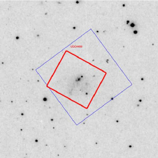
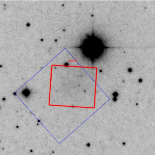
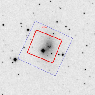
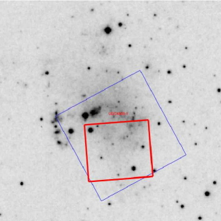
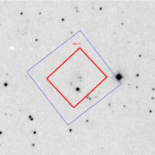
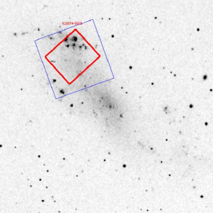
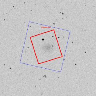
Figure 1.— Position of the WFC3/IR field of view (red), overlayed on an optical image from the Digitized Sky Survey. Blue region shows the area covered by optical HST data. (Target names from upper left to lower right: [a] UGC4459; [b] DDO78; [c] DDO82; [d] UGC5139; [e] UGC4305-1; [f] UGC4305-2; [g] HS117; [h] IC2574-SGS; [i] ESO540-030;).

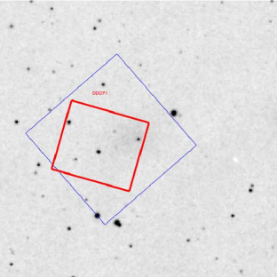
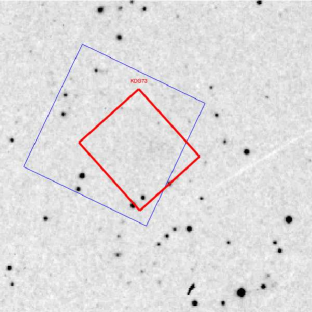
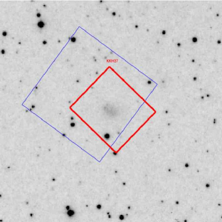
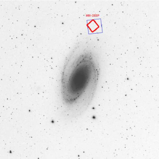
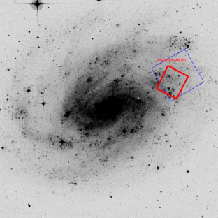
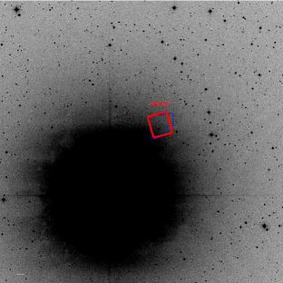
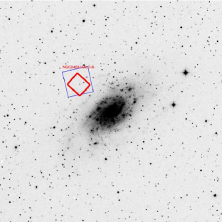
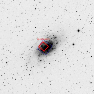
Figure 1 continued.— Position of the WFC3/IR field of view (red), overlayed on an optical image from the Digitized Sky Survey. Blue region shows the area covered by optical HST data. (Target names from upper left to lower right: [j] DDO71; [k] KDG73; [l] KKH37; [m] M81-DEEP; [n] NGC0300-WIDE1; [o] NGC404; [p] NGC2403-DEEP; [q] NGC2403-HALO-6; [r] SN-NGC2403-PR;).

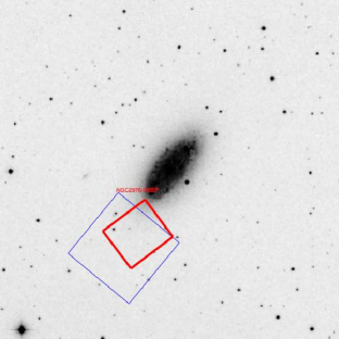
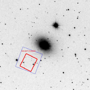
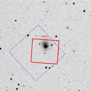
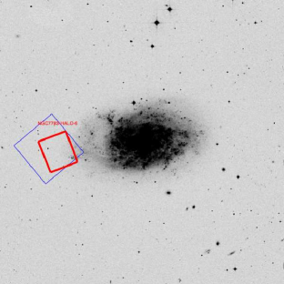
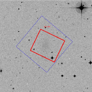
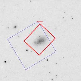
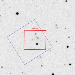
Figure 1 continued.— Position of the WFC3/IR field of view (red), overlayed on an optical image from the Digitized Sky Survey. Blue region shows the area covered by optical HST data. (Target names from upper left to lower right: [s] NGC2976-DEEP; [t] NGC3077-PHOENIX; [u] NGC3741; [v] NGC4163; [w] NGC7793-HALO-6; [x] SCL-DE1; [y] UGC8508; [z] UGCA292;).

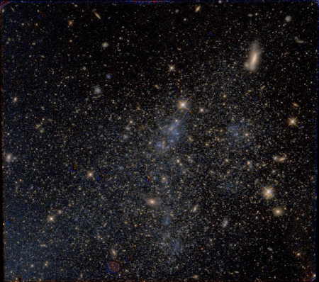
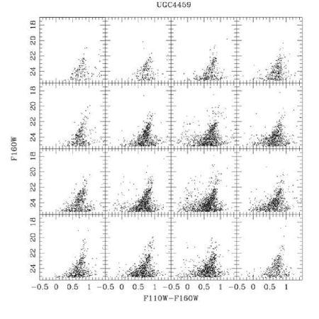
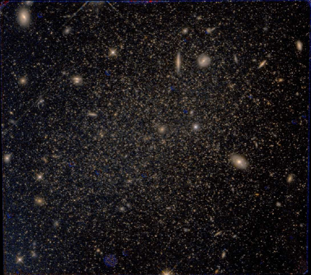
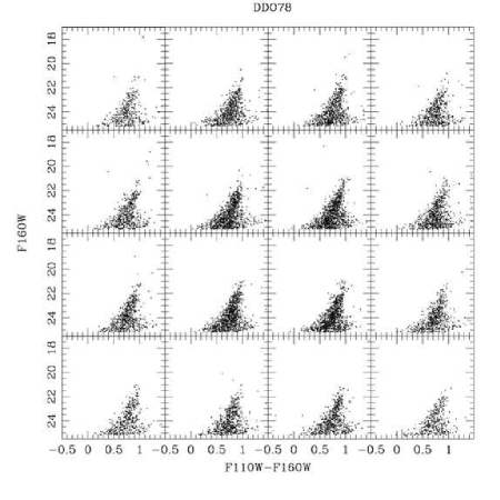
Figure 4.— (Left) False color $F110W+F160W$ image of the WFC3/IR field for the target UGC4459 within the galaxy DDO53 [Top] and within the galaxy DDO78 [Bottom]. (Right) Color-magnitude diagrams generated for a grid of subregions, so that the upper left CMD corresponds to the upper left of the adjacent image.

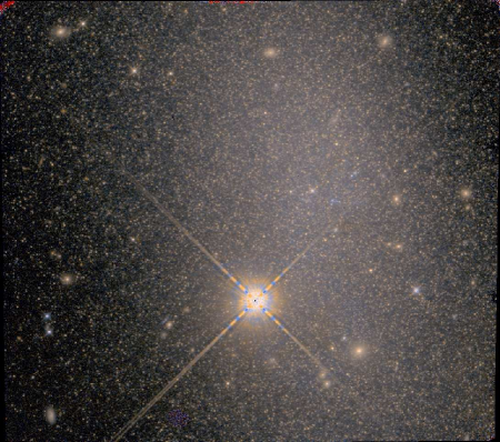
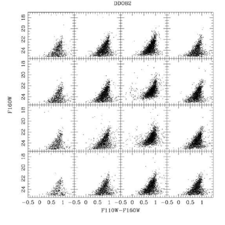
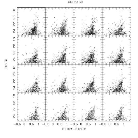
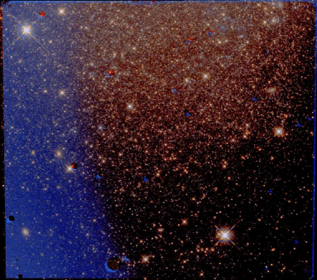
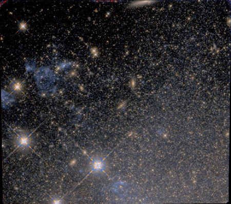
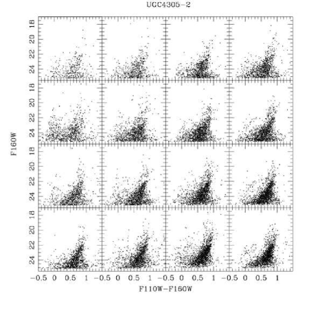
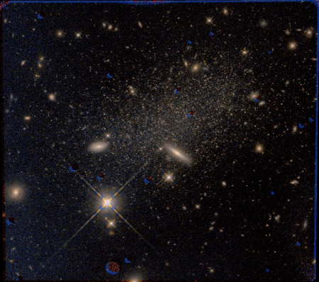
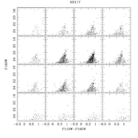
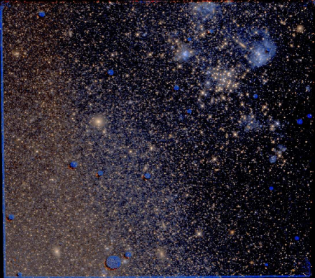
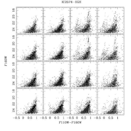
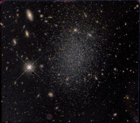
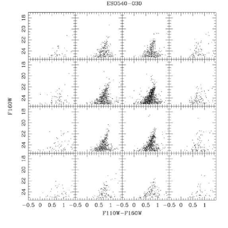
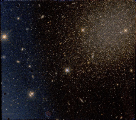
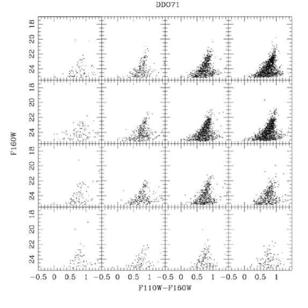
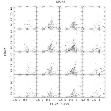
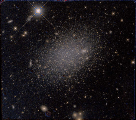
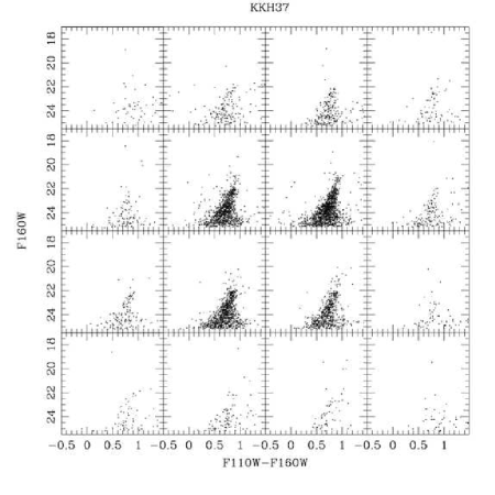
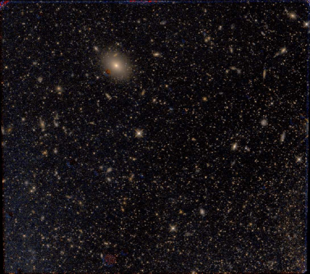
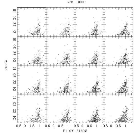
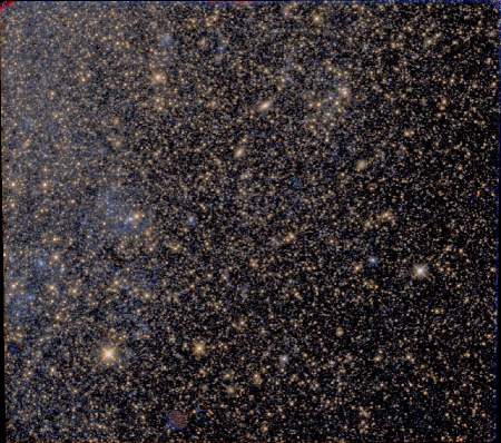
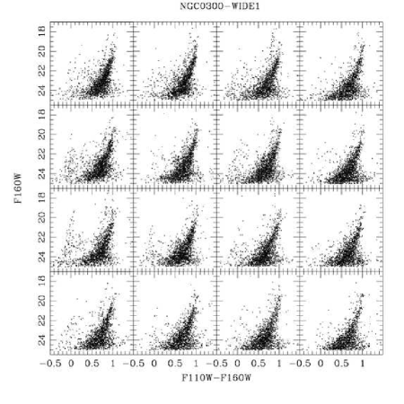
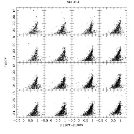
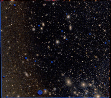
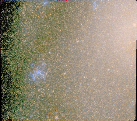
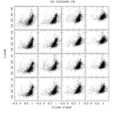
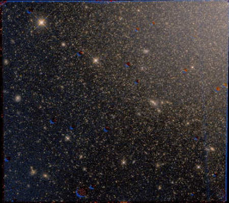
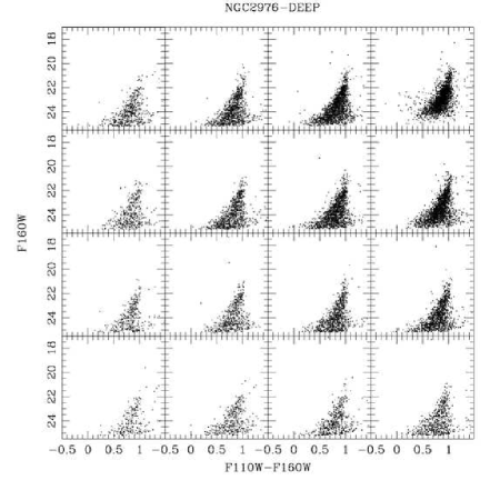
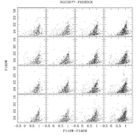
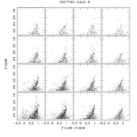
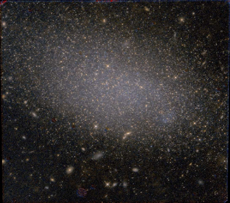
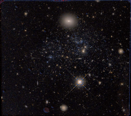
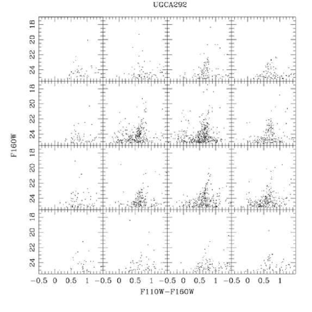
Figure 4 continued.— (Left) False color $F110W+F160W$ image of the WFC3/IR field for within the galaxy DDO82 [Top] and the target UGC5139 within the galaxy HoI [Bottom]. (Right) Color-magnitude diagrams generated for a grid of subregions, so that the upper left CMD corresponds to the upper left of the adjacent image.

Figure 4 continued.— (Left) False color $F110W+F160W$ image of the WFC3/IR field for the target UGC4305-1 within the galaxy HoII [Top] and the target UGC4305-2 within the galaxy HoII [Bottom]. (Right) Color-magnitude diagrams generated for a grid of subregions, so that the upper left CMD corresponds to the upper left of the adjacent image.

Figure 4 continued.— (Left) False color $F110W+F160W$ image of the WFC3/IR field for within the galaxy HS117 [Top] and the target IC2574-SGS within the galaxy I2574 [Bottom]. (Right) Color-magnitude diagrams generated for a grid of subregions, so that the upper left CMD corresponds to the upper left of the adjacent image.

Figure 4 continued.— (Left) False color $F110W+F160W$ image of the WFC3/IR field for the target ESO540-030 within the galaxy KDG2 [Top] and the target DDO71 within the galaxy KDG63 [Bottom]. (Right) Color-magnitude diagrams generated for a grid of subregions, so that the upper left CMD corresponds to the upper left of the adjacent image.

Figure 4 continued.— (Left) False color $F110W+F160W$ image of the WFC3/IR field for within the galaxy KDG73 [Top] and within the galaxy KKH37 [Bottom]. (Right) Color-magnitude diagrams generated for a grid of subregions, so that the upper left CMD corresponds to the upper left of the adjacent image.

Figure 4 continued.— (Left) False color $F110W+F160W$ image of the WFC3/IR field for the target M81-DEEP within the galaxy M81 [Top] and the target NGC0300-WIDE1 within the galaxy N300 [Bottom]. (Right) Color-magnitude diagrams generated for a grid of subregions, so that the upper left CMD corresponds to the upper left of the adjacent image.

Figure 4 continued.— (Left) False color $F110W+F160W$ image of the WFC3/IR field for the target NGC404 within the galaxy N404 [Top] and the target NGC2403-DEEP within the galaxy N2403 [Bottom]. (Right) Color-magnitude diagrams generated for a grid of subregions, so that the upper left CMD corresponds to the upper left of the adjacent image.

Figure 4 continued.— (Left) False color $F110W+F160W$ image of the WFC3/IR field for the target NGC2403-HALO-6 within the galaxy N2403 [Top] and the target SN-NGC2403-PR within the galaxy N2403 [Bottom]. (Right) Color-magnitude diagrams generated for a grid of subregions, so that the upper left CMD corresponds to the upper left of the adjacent image.

Figure 4 continued.— (Left) False color $F110W+F160W$ image of the WFC3/IR field for the target NGC2976-DEEP within the galaxy N2976 [Top] and the target NGC3077-PHOENIX within the galaxy N3077 [Bottom]. (Right) Color-magnitude diagrams generated for a grid of subregions, so that the upper left CMD corresponds to the upper left of the adjacent image.

Figure 4 continued.— (Left) False color $F110W+F160W$ image of the WFC3/IR field for the target NGC3741 within the galaxy N3741 [Top] and the target NGC4163 within the galaxy N4163 [Bottom]. (Right) Color-magnitude diagrams generated for a grid of subregions, so that the upper left CMD corresponds to the upper left of the adjacent image.

Figure 4 continued.— (Left) False color $F110W+F160W$ image of the WFC3/IR field for the target NGC7793-HALO-6 within the galaxy N7793 [Top] and the target SCL-DE1 within the galaxy Sc22 [Bottom]. (Right) Color-magnitude diagrams generated for a grid of subregions, so that the upper left CMD corresponds to the upper left of the adjacent image.

Figure 4 continued.— (Left) False color $F110W+F160W$ image of the WFC3/IR field for the target UGC8508 within the galaxy U8508 [Top] and the target UGCA292 within the galaxy UA292 [Bottom]. (Right) Color-magnitude diagrams generated for a grid of subregions, so that the upper left CMD corresponds to the upper left of the adjacent image.

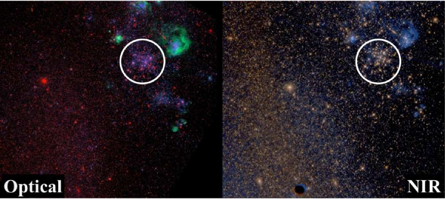
Figure 17.— Comparison between a false-color image in the optical (left: $F435W+F555W+F814W$) and the NIR (right: $F110W+F160W$) in a star forming region of I2574. Nebulosity associated with line emission from ionized [Siii] and netural He is visible near Hii regions in the NIR image. The circle indicates a compact star formation region dominated by luminous red core-Helium burning (RHeB) stars. This SF region is old enough that the photoionized Hii has recombined ($\gtrsim 10{\rm\,Myrs}$), and therefore lacks the diffuse emission seen in the younger neighboring HII regions. However, it also hosts all of the most NIR luminous sources (see discussion in Section 3.2.2).

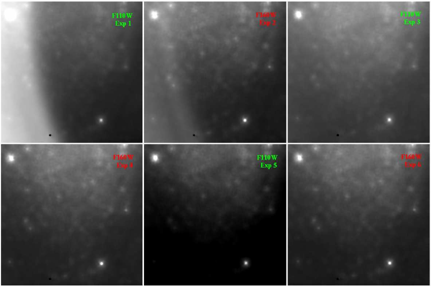
Figure 18.— DOLPHOT’s estimate of the local sky for a sequence of exposures taken during a single orbit visit for UGC4305-1, based on DOLPHOT’s PSF fitting. The first exposure in the orbit is in the upper left, and the final exposure is in the lower right. Exposures alternate between $F110W$ and $F160W$, and all images for a single filter have been displayed with a common scale and stretch. There is an overall gradient from top to bottom in all images, due to a larger fraction of unresolved sources in the upper half of the image. There is also a time-dependent feature on the left hand side of the image, due to scattered light. We show in Figure 19 that this feature appears when the telescope is pointed to within $30{{}^{\circ}}$ of a bright earth limb; the first two exposures in the orbit had average limb angles of $22{{}^{\circ}}$ and $26{{}^{\circ}}$, respectively, while the third through sixth exposures have limb angles of $31{{}^{\circ}}$, $34{{}^{\circ}}$, $36{{}^{\circ}}$, and $37{{}^{\circ}}$, respectively. Even after the bright limb feature disappears, there are still temporal variations in the overall sky brightness level.

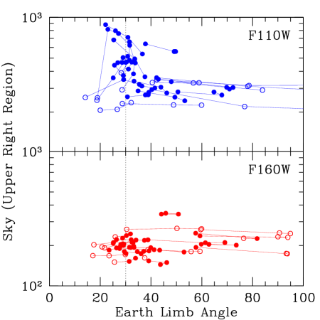
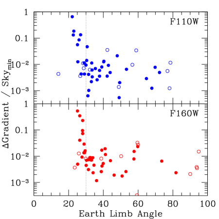
Figure 19.— (Left) Sky level (counts per pixel) in the upper right quadrant of all $F110W$ and $F160W$ exposures (top and bottom, respectively), as a function of the average angle between the spacecraft’s V1 axis and the earth’s limb during the exposure; open circles indicate that the limb was dark at the time of observation. Successive exposures in a single orbit are connected by lines, but intermediate non-destructive reads are not shown. In $F110W$, the mean sky level is clearly correlated with proximity to the earth’s limb, when the limb is bright. (Right) The amplitude of the scattered light feature seen in Figure 18 (as a fraction of the sky brightness), as a function of the average angle to the earth’s limb during each observation. The amplitude of the scattered light feature is taken to be the excess counts in the affected region, compared to the variation in the mean sky level seen in the unaffected upper right quadrant. It is calculated by first calculating a gradient across the image using the difference between the amplitude of the sky in the affected region and the unaffected region in the upper right of the image. The smallest gradient for the exposures in a given orbit is then taken to be the expected true spatial variation in the sky background, in the absence of scattered light. The amplitude of the scattered light feature is then scaled to the level of the sky in the upper right quadrant of each image, giving the approximate amplitude of the feature as a percent of sky. The scattered light feature turns on abruptly at earth limb angles less than 30^∘.

Figure 20.— Photometric uncertainties as a function of magnitude in the $F110W$ (top) and $F160W$ filters, for a representative field with moderate crowding (UGC8508), using the more complete *.st catalog. The vertical lines indicate the average 50% completeness level determined from artificial star tests (Table 2). Photometric uncertainties are those reported by DOLPHOT, and do not fully capture the uncertainties due to crowding (see Figure 22).

Figure 21.— Comparison of the color magnitude diagrams of the original stellar *.st photometry (left) and the high quality “cleaned” *.gst photometry (right) for target IC2574-SGS. The original photometry has higher completeness, but at the expense of increased errors due to crowding, producing less sharp features in the CMD. The *.st photometry includes stars that have a signal-to-noise of greater than 4 in only one filter, making the colors unreliable at faint magnitudes; the *.gst photometry requires high signal-to-noise in both filters.

Figure 22.— Distribution of differences between the true and the recovered $F160W$ magnitudes for artificial stars inserted into images of IC2574-SGS (left; highly crowded) and UGC 4459 (right; uncrowded). Distributions are calculated in bins 1 magnitude wide, with increasing line thicknesses indicating fainter magnitudes; the heaviest line includes stars with $23<m_{\rm{F160W}}\leq 24$. Crowding biases the photometry very slightly ($<0.004\,$mag) towards fainter observed magnitudes at the median, with larger biases at fainter magnitudes. However, these biases are much smaller than the photometric errors ($<\!0.05\sigma_{m}$ for IC2574-SGS) in all magnitude ranges. The uncertainties in the magnitude of individual stars is frequently dominated by crowding, however (see Figure 20 for typical photometric errors as a function of magnitude.)

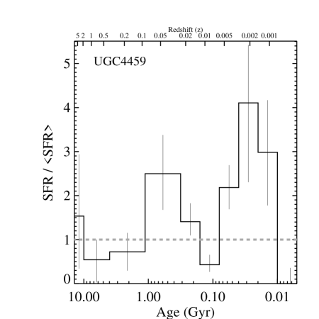
Figure 23.— Color magnitude diagrams of the WFC3/IR (upper left) and optical (upper right) for the target UGC4459 within galaxy DDO53. Lower panels show the star formation history derived from the optical data, for both the differential (left, with horizontal dotted line indicating the past average SFR) and cumulative (right) star formation histories. The cumulative star formation history is calculated from the present back to 14 Gyrs. Uncertainties in the lower two panels are the 68% confidence intervals, calculated from Monte Carlo tests including random and systematic uncertainties. Optical CMDs are restricted to the area covered by the WFC3 FOV.

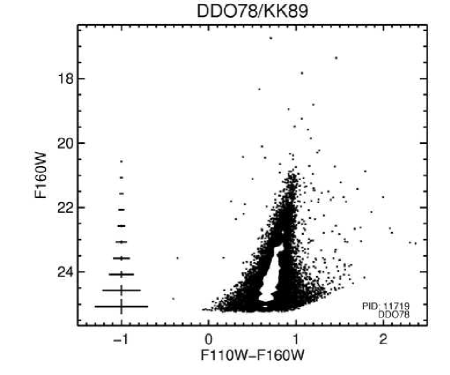
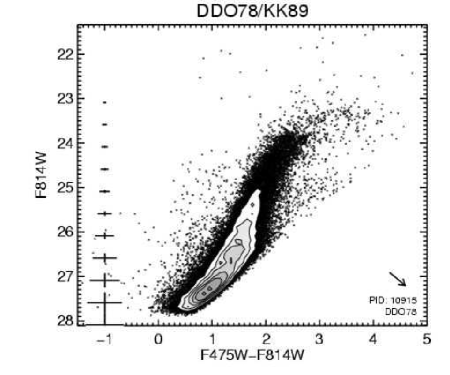
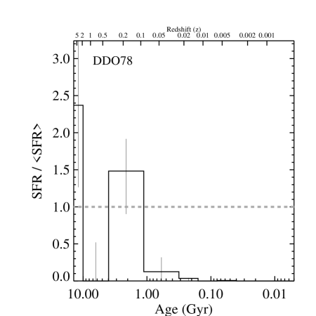
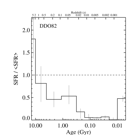
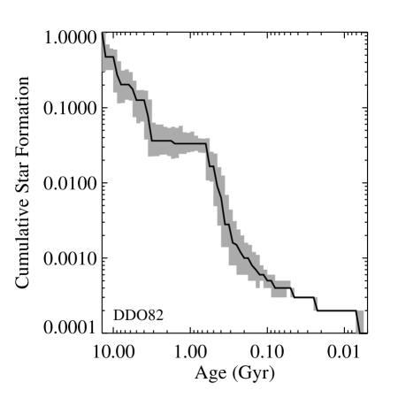
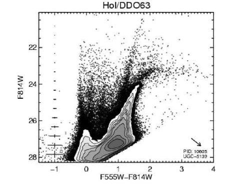
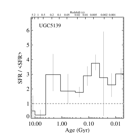
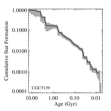
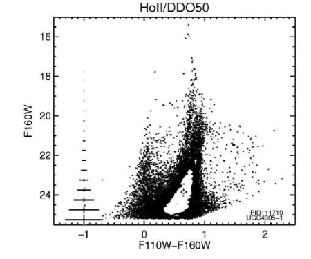
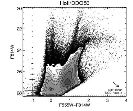
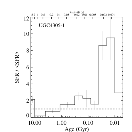
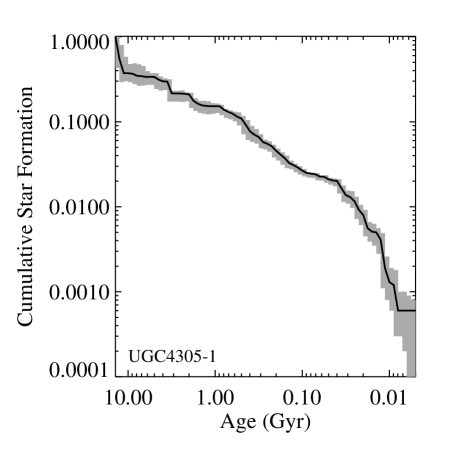
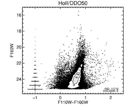
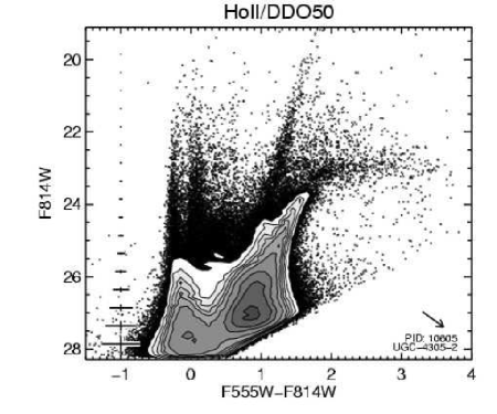
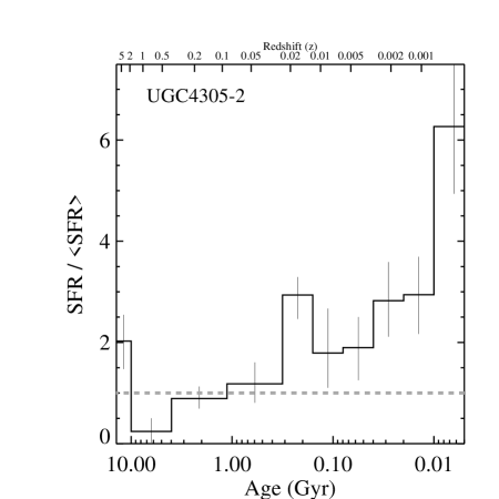
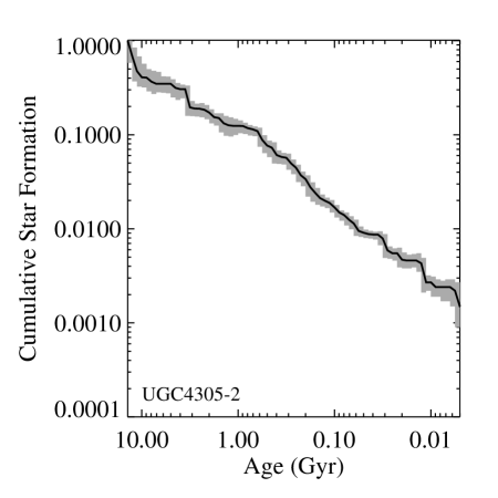
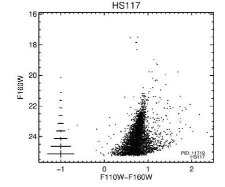
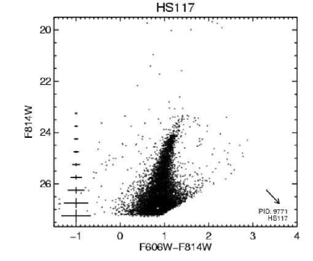
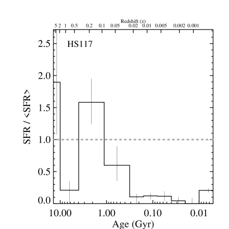
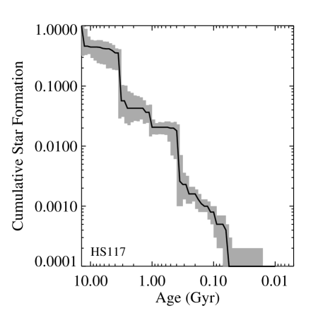
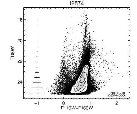
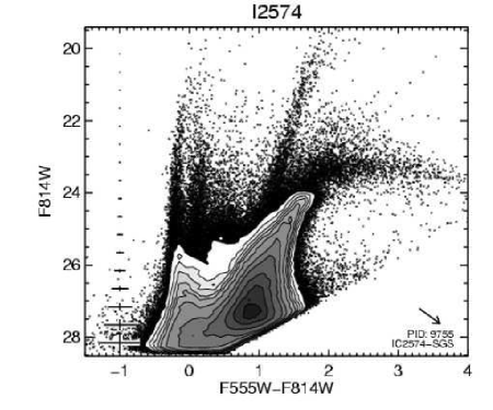
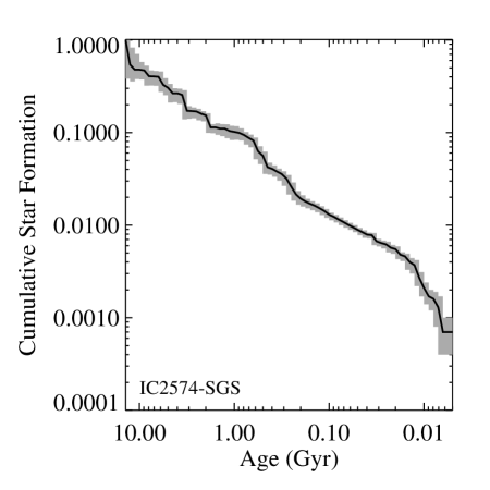
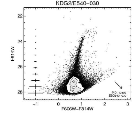
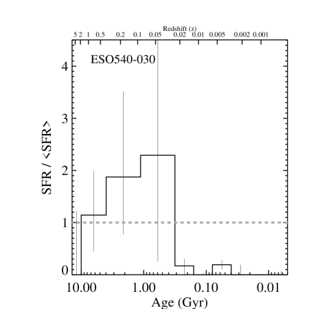
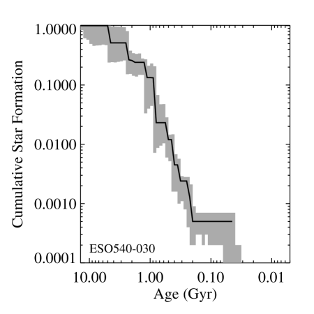
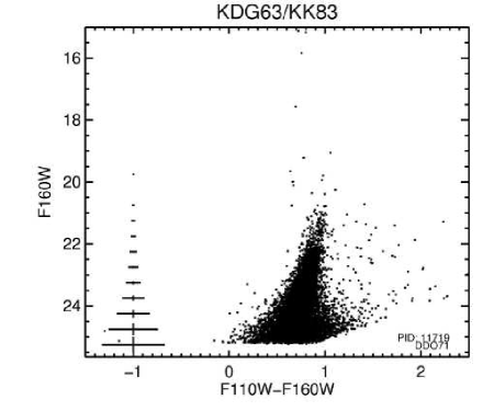
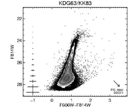
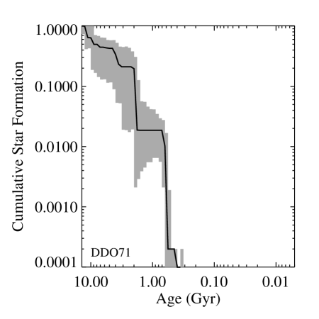
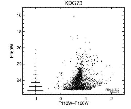
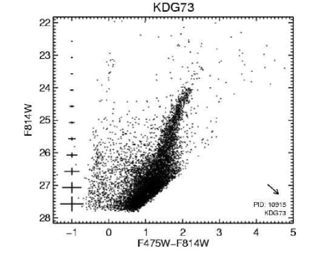
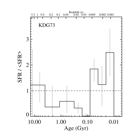
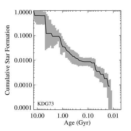
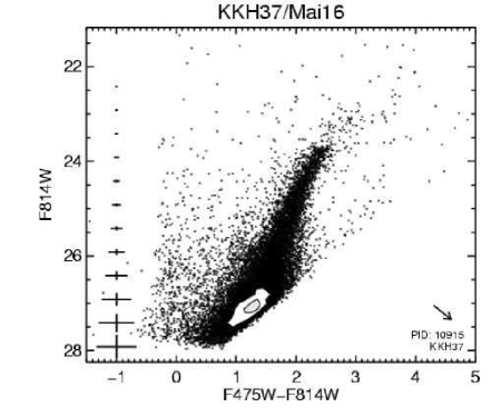
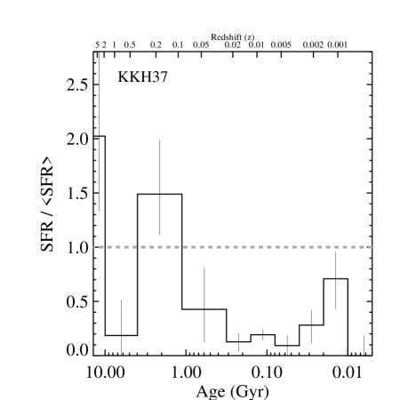
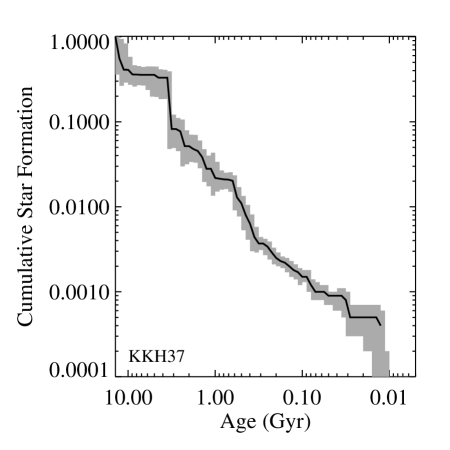
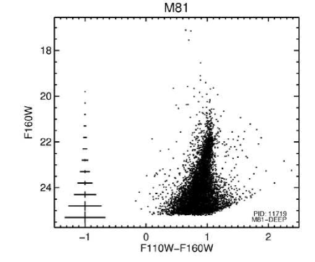
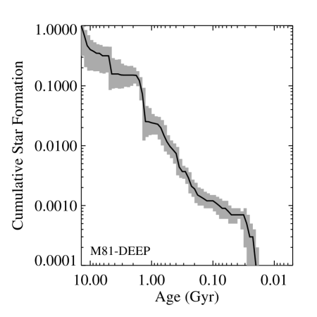
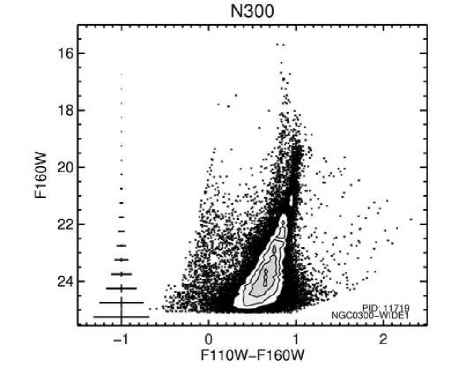
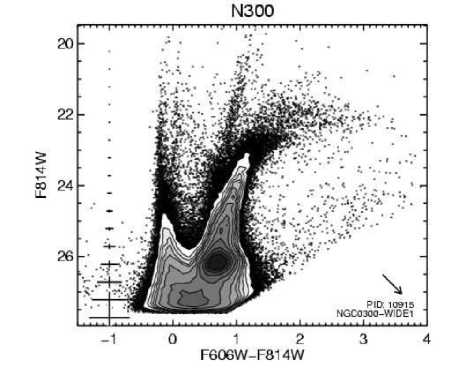
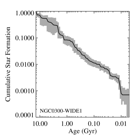
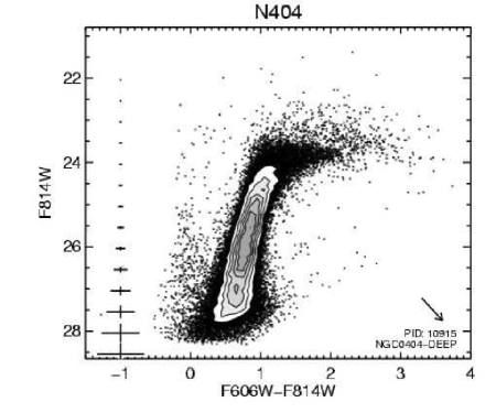
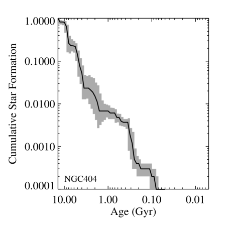
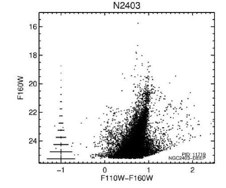
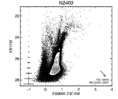
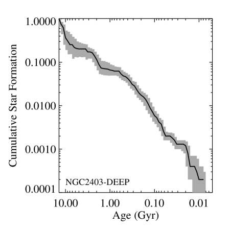
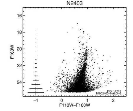
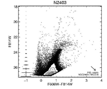
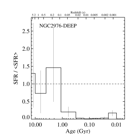
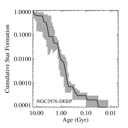
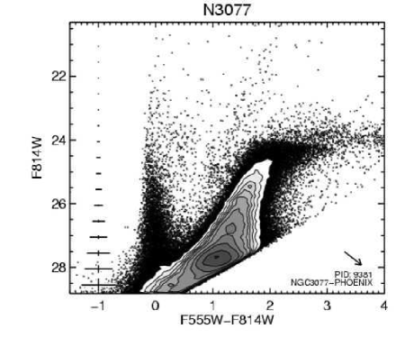
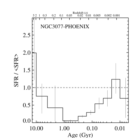
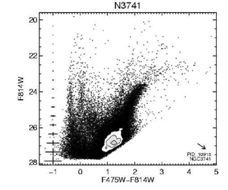
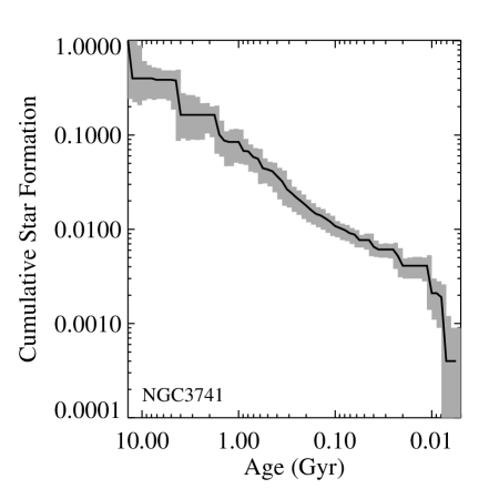
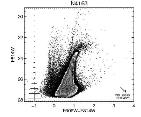
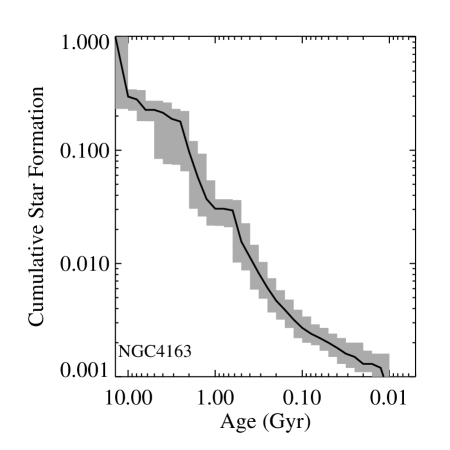
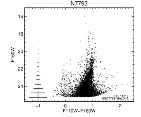
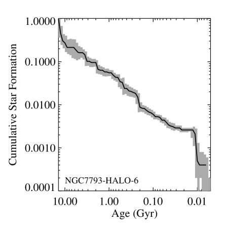
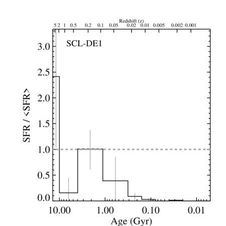
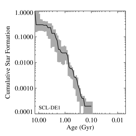
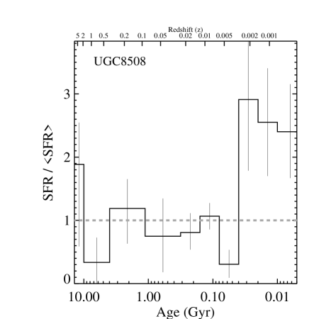
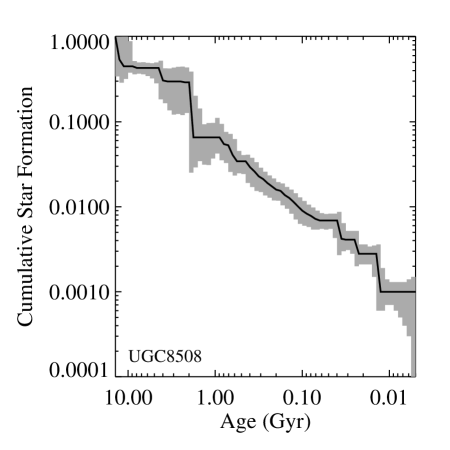
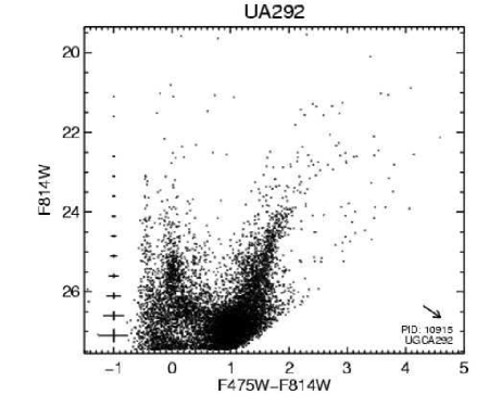
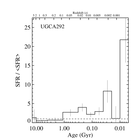
Figure 23 continued.— Color magnitude diagrams of the WFC3/IR (upper left) and optical (upper right) for DDO78. Lower panels show the star formation history derived from the optical data, for both the differential (left, with horizontal dotted line indicating the past average SFR) and cumulative (right) star formation histories. The cumulative star formation history is calculated from the present back to 14 Gyrs. Uncertainties in the lower two panels are the 68% confidence intervals, calculated from Monte Carlo tests including random and systematic uncertainties. Optical CMDs are restricted to the area covered by the WFC3 FOV.

Figure 23 continued.— Color magnitude diagrams of the WFC3/IR (upper left) and optical (upper right) for DDO82. Lower panels show the star formation history derived from the optical data, for both the differential (left, with horizontal dotted line indicating the past average SFR) and cumulative (right) star formation histories. The cumulative star formation history is calculated from the present back to 14 Gyrs. Uncertainties in the lower two panels are the 68% confidence intervals, calculated from Monte Carlo tests including random and systematic uncertainties. Optical CMDs are restricted to the area covered by the WFC3 FOV.

Figure 23 continued.— Color magnitude diagrams of the WFC3/IR (upper left) and optical (upper right) for the target UGC5139 within galaxy HoI. Lower panels show the star formation history derived from the optical data, for both the differential (left, with horizontal dotted line indicating the past average SFR) and cumulative (right) star formation histories. The cumulative star formation history is calculated from the present back to 14 Gyrs. Uncertainties in the lower two panels are the 68% confidence intervals, calculated from Monte Carlo tests including random and systematic uncertainties. Optical CMDs are restricted to the area covered by the WFC3 FOV.

Figure 23 continued.— Color magnitude diagrams of the WFC3/IR (upper left) and optical (upper right) for the target UGC4305-1 within galaxy HoII. Lower panels show the star formation history derived from the optical data, for both the differential (left, with horizontal dotted line indicating the past average SFR) and cumulative (right) star formation histories. The cumulative star formation history is calculated from the present back to 14 Gyrs. Uncertainties in the lower two panels are the 68% confidence intervals, calculated from Monte Carlo tests including random and systematic uncertainties. Optical CMDs are restricted to the area covered by the WFC3 FOV.

Figure 23 continued.— Color magnitude diagrams of the WFC3/IR (upper left) and optical (upper right) for the target UGC4305-2 within galaxy HoII. Lower panels show the star formation history derived from the optical data, for both the differential (left, with horizontal dotted line indicating the past average SFR) and cumulative (right) star formation histories. The cumulative star formation history is calculated from the present back to 14 Gyrs. Uncertainties in the lower two panels are the 68% confidence intervals, calculated from Monte Carlo tests including random and systematic uncertainties. Optical CMDs are restricted to the area covered by the WFC3 FOV.

Figure 23 continued.— Color magnitude diagrams of the WFC3/IR (upper left) and optical (upper right) for HS117. Lower panels show the star formation history derived from the optical data, for both the differential (left, with horizontal dotted line indicating the past average SFR) and cumulative (right) star formation histories. The cumulative star formation history is calculated from the present back to 14 Gyrs. Uncertainties in the lower two panels are the 68% confidence intervals, calculated from Monte Carlo tests including random and systematic uncertainties. Optical CMDs are restricted to the area covered by the WFC3 FOV.

Figure 23 continued.— Color magnitude diagrams of the WFC3/IR (upper left) and optical (upper right) for the target IC2574-SGS within galaxy I2574. Lower panels show the star formation history derived from the optical data, for both the differential (left, with horizontal dotted line indicating the past average SFR) and cumulative (right) star formation histories. The cumulative star formation history is calculated from the present back to 14 Gyrs. Uncertainties in the lower two panels are the 68% confidence intervals, calculated from Monte Carlo tests including random and systematic uncertainties. Optical CMDs are restricted to the area covered by the WFC3 FOV.

Figure 23 continued.— Color magnitude diagrams of the WFC3/IR (upper left) and optical (upper right) for the target ESO540-030 within galaxy KDG2. Lower panels show the star formation history derived from the optical data, for both the differential (left, with horizontal dotted line indicating the past average SFR) and cumulative (right) star formation histories. The cumulative star formation history is calculated from the present back to 14 Gyrs. Uncertainties in the lower two panels are the 68% confidence intervals, calculated from Monte Carlo tests including random and systematic uncertainties. Optical CMDs are restricted to the area covered by the WFC3 FOV.

Figure 23 continued.— Color magnitude diagrams of the WFC3/IR (upper left) and optical (upper right) for the target DDO71 within galaxy KDG63. Lower panels show the star formation history derived from the optical data, for both the differential (left, with horizontal dotted line indicating the past average SFR) and cumulative (right) star formation histories. The cumulative star formation history is calculated from the present back to 14 Gyrs. Uncertainties in the lower two panels are the 68% confidence intervals, calculated from Monte Carlo tests including random and systematic uncertainties. Optical CMDs are restricted to the area covered by the WFC3 FOV.

Figure 23 continued.— Color magnitude diagrams of the WFC3/IR (upper left) and optical (upper right) for KDG73. Lower panels show the star formation history derived from the optical data, for both the differential (left, with horizontal dotted line indicating the past average SFR) and cumulative (right) star formation histories. The cumulative star formation history is calculated from the present back to 14 Gyrs. Uncertainties in the lower two panels are the 68% confidence intervals, calculated from Monte Carlo tests including random and systematic uncertainties. Optical CMDs are restricted to the area covered by the WFC3 FOV.

Figure 23 continued.— Color magnitude diagrams of the WFC3/IR (upper left) and optical (upper right) for KKH37. Lower panels show the star formation history derived from the optical data, for both the differential (left, with horizontal dotted line indicating the past average SFR) and cumulative (right) star formation histories. The cumulative star formation history is calculated from the present back to 14 Gyrs. Uncertainties in the lower two panels are the 68% confidence intervals, calculated from Monte Carlo tests including random and systematic uncertainties. Optical CMDs are restricted to the area covered by the WFC3 FOV.

Figure 23 continued.— Color magnitude diagrams of the WFC3/IR (upper left) and optical (upper right) for the target M81-DEEP within galaxy M81. Lower panels show the star formation history derived from the optical data, for both the differential (left, with horizontal dotted line indicating the past average SFR) and cumulative (right) star formation histories. The cumulative star formation history is calculated from the present back to 14 Gyrs. Uncertainties in the lower two panels are the 68% confidence intervals, calculated from Monte Carlo tests including random and systematic uncertainties. Optical CMDs are restricted to the area covered by the WFC3 FOV.

Figure 23 continued.— Color magnitude diagrams of the WFC3/IR (upper left) and optical (upper right) for the target NGC0300-WIDE1 within galaxy N300. Lower panels show the star formation history derived from the optical data, for both the differential (left, with horizontal dotted line indicating the past average SFR) and cumulative (right) star formation histories. The cumulative star formation history is calculated from the present back to 14 Gyrs. Uncertainties in the lower two panels are the 68% confidence intervals, calculated from Monte Carlo tests including random and systematic uncertainties. Optical CMDs are restricted to the area covered by the WFC3 FOV.

Figure 23 continued.— Color magnitude diagrams of the WFC3/IR (upper left) and optical (upper right) for the target NGC404 within galaxy N404. Lower panels show the star formation history derived from the optical data, for both the differential (left, with horizontal dotted line indicating the past average SFR) and cumulative (right) star formation histories. The cumulative star formation history is calculated from the present back to 14 Gyrs. Uncertainties in the lower two panels are the 68% confidence intervals, calculated from Monte Carlo tests including random and systematic uncertainties. Optical CMDs are restricted to the area covered by the WFC3 FOV.

Figure 23 continued.— Color magnitude diagrams of the WFC3/IR (upper left) and optical (upper right) for the target NGC2403-DEEP within galaxy N2403. Lower panels show the star formation history derived from the optical data, for both the differential (left, with horizontal dotted line indicating the past average SFR) and cumulative (right) star formation histories. The cumulative star formation history is calculated from the present back to 14 Gyrs. Uncertainties in the lower two panels are the 68% confidence intervals, calculated from Monte Carlo tests including random and systematic uncertainties. Optical CMDs are restricted to the area covered by the WFC3 FOV.

Figure 23 continued.— Color magnitude diagrams of the WFC3/IR (upper left) and optical (upper right) for the target NGC2403-HALO-6 within galaxy N2403. Lower panels show the star formation history derived from the optical data, for both the differential (left, with horizontal dotted line indicating the past average SFR) and cumulative (right) star formation histories. The cumulative star formation history is calculated from the present back to 14 Gyrs. Uncertainties in the lower two panels are the 68% confidence intervals, calculated from Monte Carlo tests including random and systematic uncertainties. Optical CMDs are restricted to the area covered by the WFC3 FOV.

Figure 23 continued.— Color magnitude diagrams of the WFC3/IR (upper left) and optical (upper right) for the target SN-NGC2403-PR within galaxy N2403. Lower panels show the star formation history derived from the optical data, for both the differential (left, with horizontal dotted line indicating the past average SFR) and cumulative (right) star formation histories. The cumulative star formation history is calculated from the present back to 14 Gyrs. Uncertainties in the lower two panels are the 68% confidence intervals, calculated from Monte Carlo tests including random and systematic uncertainties. Optical CMDs are restricted to the area covered by the WFC3 FOV.

Figure 23 continued.— Color magnitude diagrams of the WFC3/IR (upper left) and optical (upper right) for the target NGC2976-DEEP within galaxy N2976. Lower panels show the star formation history derived from the optical data, for both the differential (left, with horizontal dotted line indicating the past average SFR) and cumulative (right) star formation histories. The cumulative star formation history is calculated from the present back to 14 Gyrs. Uncertainties in the lower two panels are the 68% confidence intervals, calculated from Monte Carlo tests including random and systematic uncertainties. Optical CMDs are restricted to the area covered by the WFC3 FOV.

Figure 23 continued.— Color magnitude diagrams of the WFC3/IR (upper left) and optical (upper right) for the target NGC3077-PHOENIX within galaxy N3077. Lower panels show the star formation history derived from the optical data, for both the differential (left, with horizontal dotted line indicating the past average SFR) and cumulative (right) star formation histories. The cumulative star formation history is calculated from the present back to 14 Gyrs. Uncertainties in the lower two panels are the 68% confidence intervals, calculated from Monte Carlo tests including random and systematic uncertainties. Optical CMDs are restricted to the area covered by the WFC3 FOV.

Figure 23 continued.— Color magnitude diagrams of the WFC3/IR (upper left) and optical (upper right) for the target NGC3741 within galaxy N3741. Lower panels show the star formation history derived from the optical data, for both the differential (left, with horizontal dotted line indicating the past average SFR) and cumulative (right) star formation histories. The cumulative star formation history is calculated from the present back to 14 Gyrs. Uncertainties in the lower two panels are the 68% confidence intervals, calculated from Monte Carlo tests including random and systematic uncertainties. Optical CMDs are restricted to the area covered by the WFC3 FOV.

Figure 23 continued.— Color magnitude diagrams of the WFC3/IR (upper left) and optical (upper right) for the target NGC4163 within galaxy N4163. Lower panels show the star formation history derived from the optical data, for both the differential (left, with horizontal dotted line indicating the past average SFR) and cumulative (right) star formation histories. The cumulative star formation history is calculated from the present back to 14 Gyrs. Uncertainties in the lower two panels are the 68% confidence intervals, calculated from Monte Carlo tests including random and systematic uncertainties. Optical CMDs are restricted to the area covered by the WFC3 FOV.

Figure 23 continued.— Color magnitude diagrams of the WFC3/IR (upper left) and optical (upper right) for the target NGC7793-HALO-6 within galaxy N7793. Lower panels show the star formation history derived from the optical data, for both the differential (left, with horizontal dotted line indicating the past average SFR) and cumulative (right) star formation histories. The cumulative star formation history is calculated from the present back to 14 Gyrs. Uncertainties in the lower two panels are the 68% confidence intervals, calculated from Monte Carlo tests including random and systematic uncertainties. Optical CMDs are restricted to the area covered by the WFC3 FOV.

Figure 23 continued.— Color magnitude diagrams of the WFC3/IR (upper left) and optical (upper right) for the target SCL-DE1 within galaxy Sc22. Lower panels show the star formation history derived from the optical data, for both the differential (left, with horizontal dotted line indicating the past average SFR) and cumulative (right) star formation histories. The cumulative star formation history is calculated from the present back to 14 Gyrs. Uncertainties in the lower two panels are the 68% confidence intervals, calculated from Monte Carlo tests including random and systematic uncertainties. Optical CMDs are restricted to the area covered by the WFC3 FOV.

Figure 23 continued.— Color magnitude diagrams of the WFC3/IR (upper left) and optical (upper right) for the target UGC8508 within galaxy U8508. Lower panels show the star formation history derived from the optical data, for both the differential (left, with horizontal dotted line indicating the past average SFR) and cumulative (right) star formation histories. The cumulative star formation history is calculated from the present back to 14 Gyrs. Uncertainties in the lower two panels are the 68% confidence intervals, calculated from Monte Carlo tests including random and systematic uncertainties. Optical CMDs are restricted to the area covered by the WFC3 FOV.

Figure 23 continued.— Color magnitude diagrams of the WFC3/IR (upper left) and optical (upper right) for the target UGCA292 within galaxy UA292. Lower panels show the star formation history derived from the optical data, for both the differential (left, with horizontal dotted line indicating the past average SFR) and cumulative (right) star formation histories. The cumulative star formation history is calculated from the present back to 14 Gyrs. Uncertainties in the lower two panels are the 68% confidence intervals, calculated from Monte Carlo tests including random and systematic uncertainties. Optical CMDs are restricted to the area covered by the WFC3 FOV.

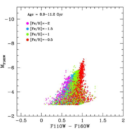
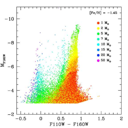
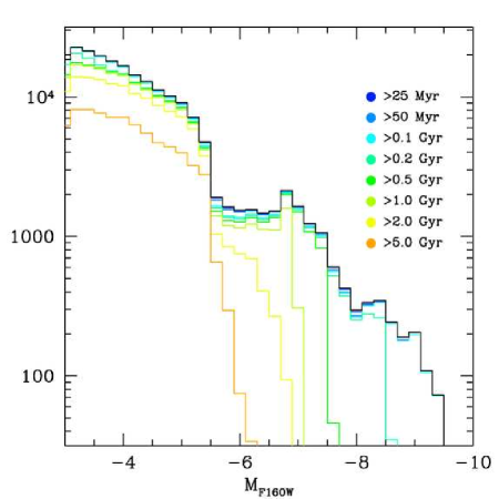
Figure 49.— Simulated CMDs showing the location of populations color-coded by age (upper left), initial stellar mass (lower left), and metallicity (upper right). The plots on the left and bottom right assume a constant star formation rate and metallicity of [Fe/H]=-1.45. The plot on the upper right assumes a constant star formation rate over a narrow age interval (8.9-11.2${\rm\,Gyr}$), for a range of metallicities. The plot on the lower right shows the total luminosity function, along with the contributions of stars older than a given stellar age, for stars and ages color coded as in the CMD on the upper left. Stars younger than $2{\rm\,Gyr}$ contribute significant numbers of NIR bright stars. Simulations use Padova isochrones with updated AGB models from Girardi et al. (2010), and assume photometric errors based on the artificial star tests for the M81-DEEP field; as we show in Melbourne et al. (2011), the current implementation of these models underestimate the constribution from red core Helium burning stars compared to the data.

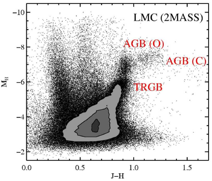
Figure 50.— $J-H$ vs $M_{H}$ 2MASS CMD for stars in the LMC. The sequence extending up from the TRGB at $M_{H}=-6$ is dominated by oxygen-rich AGB stars. The horizontal sequence at $M_{H}\sim-7.3$ extending redward of $J-H\sim 0.9$ contains mostly carbon-rich AGB stars. The main sequence is the bluest vertical sequence at $J-H\sim 0.25$. The vertical sequence at $J-H\sim 0.5$ is dominated by MW foreground stars.

Figure 51.— Simulated photometry for a model galaxy with a constant SFR and increasing metallicity (reaching $Z_{\odot}$ at the present day), made with the TRILEGAL code (Girardi et al., 2005; Girardi & Marigo, 2007). The TP-AGB population is color-coded by blue/red dots for O-rich/C-rich stars, respectively. The colors and magnitudes of C stars are derived from the model atmospheres by Loidl et al. (2001) (top row, panels a-c) or by Aringer et al. (2009) (bottom row, panels d-f). The colors of cool O-rich giants come from Fluks et al. (1994) model atmospheres. The left panels (a and d) show the expected $H$ vs. $J-H$ diagram for 2MASS filters, where C stars are found (as expected) to be slightly redder than O-rich stars. In the middle panels (b and e), however, C stars become bluer than the bulk of O-rich stars for the WFC3/IR $F160W$ vs. $F110W-F160W$ filter set, especially for the Aringer et al. (2009) models. The right panels (c and f) show the optical-IR color-color plots, comparable to Figure 54. For both models the the simulations include extended tails of blue and faint TP-AGB stars, that correspond to the $\sim 15$ % of TP-AGB stars caught in their low-luminosity dips along thermally-pulsing cycles, as well as the tails of extremely red stars at the late stages of high mass loss.

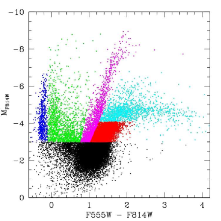
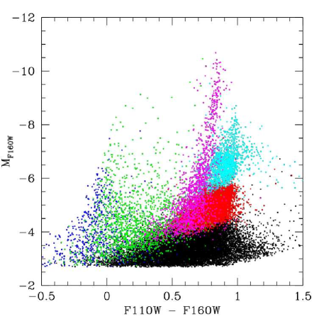
Figure 52.— Comparison of CMD features in the optical (left) and the NIR (right) for IC2574-SGS. Points are color-coded according to their likely evolutionary phase (Blue = main sequence; Green = blue core Helium burning; Magenta = red core Helium burning; Red = red giant branch; Cyan = asymptotic giant branch), as deduced from the optical CMD, for stars with $M_{F814W}<-2.5$ that are positionally well-matched to stars in the NIR; unmatched or fainter stars are plotted in black.

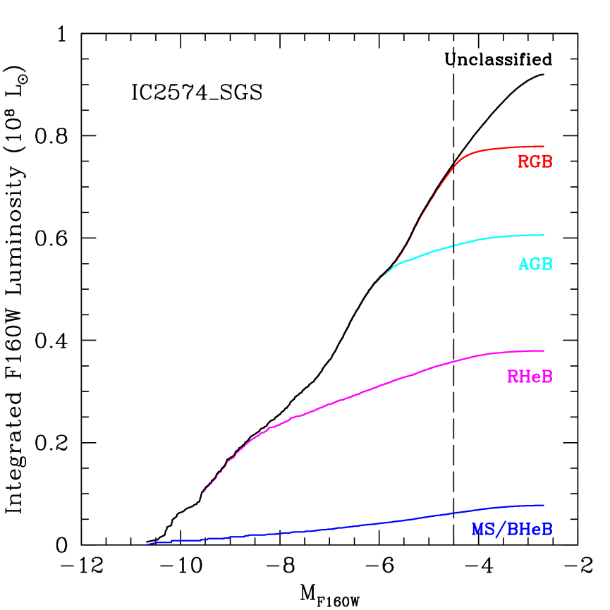
Figure 53.— Integrated $F160W$ luminosity for IC2574-SGS, integrating from the bright to the faint end, for stars classified as in Figure 52. Each line contains the integrated total luminosity for stars of a given evolutionary phase or younger, such that the “AGB” line includes the luminosity in RHeB and MS/BHeB stars as well. “Unclassified” stars are those that were not reliably matched to stars in the optical catalog. Note that the contribution from RHeB stars dominates the NIR luminosity for the detected stars. The vertical line indicates the approximate completeness limit of the data; RGB stars are likely to be the dominant contributor to the luminosity below this limit, which will reduce the fraction of the luminosity due to RHeB or AGB stars. Note that the “RGB” classification likely includes some contamination from AGB and RHeB stars as well, since such stars cannot be reliably separated within the red giant branch.

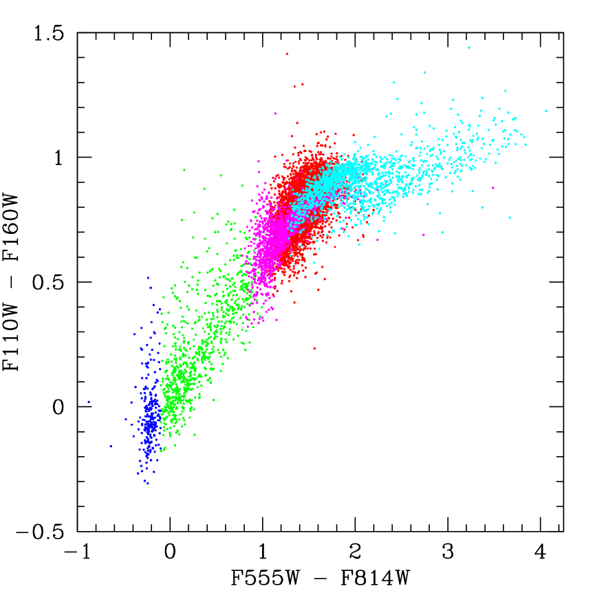
Figure 54.— Optical vs infrared color for stars within IC2574-SGS, color-coded as in Figure 52 (MS=dark blue; BHeB=green; RHeB=magenta; RGB=red; AGB=cyan). The AGB stars span a much wider range of optical colors, due to increased variability and reddening from circumstellar dust. The NIR colors of the AGB fall in a tight sequence for optical colors bluer than $F555W-F814W\!\lesssim\!1.8$, but optically redder AGB stars show increased dispersion in their NIR colors. Only stars with magnitude uncertainties of less than 0.1 mag are plotted.

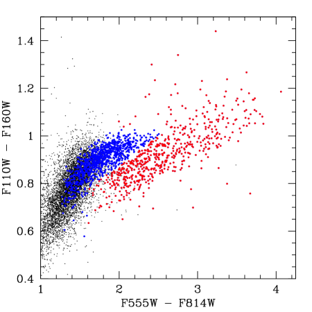
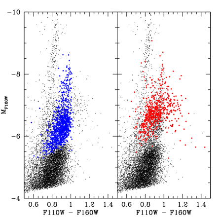
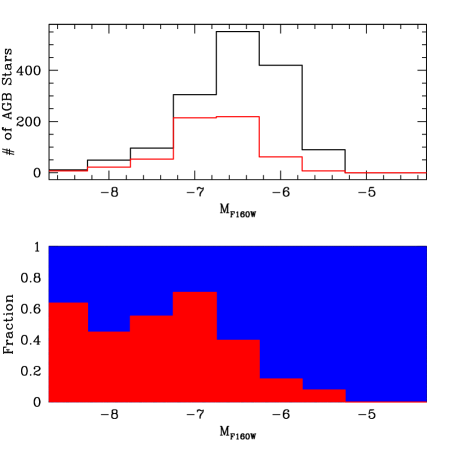
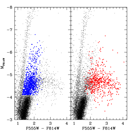
Figure 55.— (Upper Left) Color-color diagram for AGB stars from Figure 54, further split into two groups in an attempt to isolate the bluer, narrower sequence (blue points) from the redder population with high dispersion in NIR colors (red points). The NIR and optical CMDs of these two populations are shown on the upper right and lower right, respectively. The high dispersion selection isolates the reddest carbon stars (by design), and also selects against low luminosity AGB stars fainter than $M_{\rm{F160W}}=-6.5$ (histograms on lower left). The high dispersion sub-population is also systematically bluer in $F110W-F160W$ at $F160W$ magnitudes between -7 and -6.5.

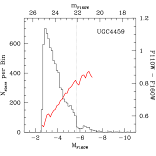
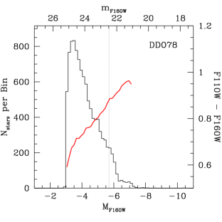
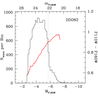
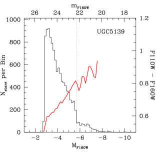
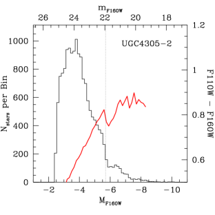
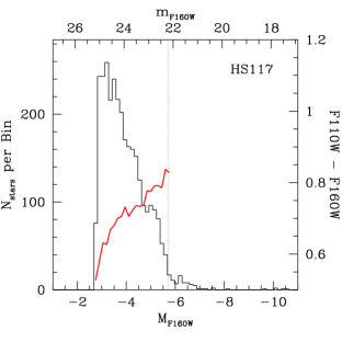
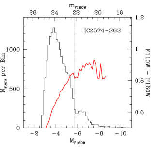
Figure 56.— Luminosity functions in $F160W$ (black histogram, left axis) and median $F110W-F160W$ color (thick red line, right axis, for bins with $>$12 stars) for red stars ( [a] DDO53; [b] DDO78; [c] DDO82; [d] HoI; [e] HoII; [f] HoII; [g] HS117; [h] I2574; [i] KDG2; ). All magnitudes have been extinction corrected, and distance moduli are as assumed in Table 1. The vertical dotted line indicates a fiducial TRGB magnitude of $F160W=-5.7$.

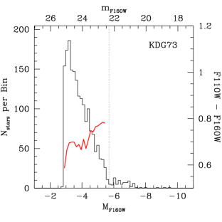
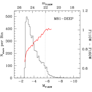
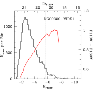
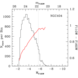
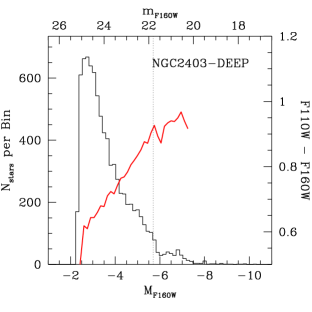
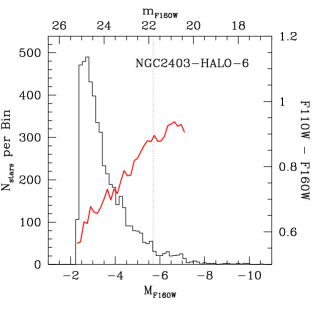
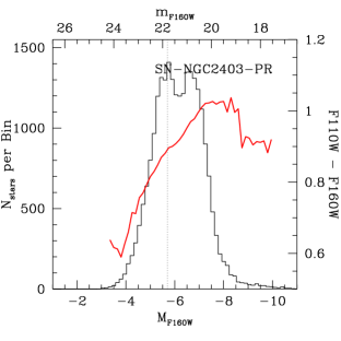
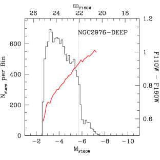
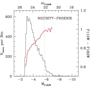
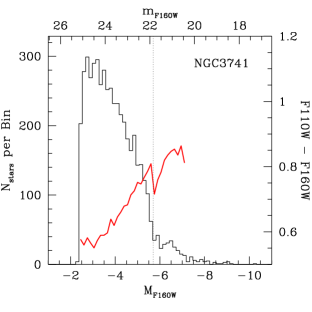
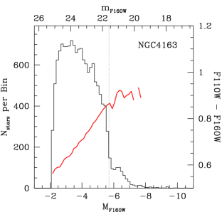
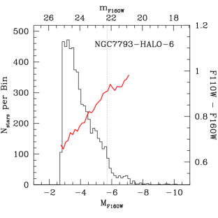
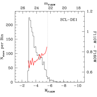
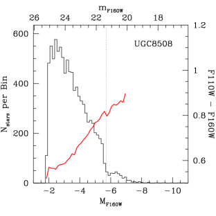
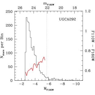
Figure 56 continued.— Luminosity functions in $F160W$ (black histogram, left axis) and median $F110W-F160W$ color (thick red line, right axis, for bins with $>$12 stars) for red stars ( [j] KDG63; [k] KDG73; [l] KKH37; [m] M81; [n] N300; [o] N404; [p] N2403; [q] N2403; [r] N2403; ). All magnitudes have been extinction corrected, and distance moduli are as assumed in Table 1. The vertical dotted line indicates a fiducial TRGB magnitude of $F160W=-5.7$.

Figure 56 continued.— Luminosity functions in $F160W$ (black histogram, left axis) and median $F110W-F160W$ color (thick red line, right axis, for bins with $>$12 stars) for red stars ( [s] N2976; [t] N3077; [u] N3741; [v] N4163; [w] N7793; [x] Sc22; [y] U8508; [z] UA292; ). All magnitudes have been extinction corrected, and distance moduli are as assumed in Table 1. The vertical dotted line indicates a fiducial TRGB magnitude of $F160W=-5.7$.

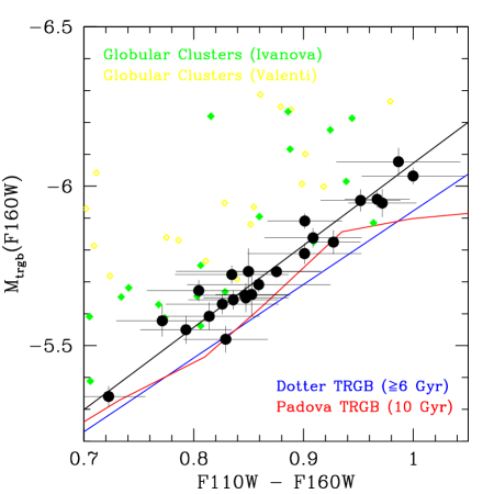
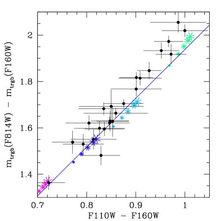
Figure 59.— (Left) Absolute $F160W$ magnitude of the TRGB as a function of $F110W-F160W$ color, for data in this sample (solid black circles). Also shown are loci from the isochrone models of Girardi et al. (2008) for a $10{\rm\,Gyr}$ RGB with a range of metallicities (solid red line; updated to the WFC3/IR filter set), and a fit to isochrone models provided by A. Dotter (blue solid line; private communication). Diamonds are data from globular clusters (solid green points are from Ivanov & Borissova 2002; open yellow points are from Valenti et al 2004,2007). Our measurements are slightly offset from the models by roughly 0.15 magnitudes brighter in $F160W$, or 0.1 magnitudes bluer in color. (Right) Magnitude difference between the optical $F814W$ (from Dalcanton et al 2009) and NIR $F160W$ TRGB, as a function of the measured $F110W-F160W$ color of the TRGB. Lines and symbols are the same as in the left hand plot. Individual points for the Dotter isochrone TRGB values are plotted for ages of 6, 8, 10, 12, & $14{\rm\,Gyr}$ (increasing asterix sizes) and metallicities of [Fe/H]=-2.49, [$\alpha$/Fe]=0.40, $Y$=0.245 (magenta), [Fe/H]=-1.99, [$\alpha$/Fe]=0.40, $Y$=0.246 (blue), [Fe/H]=-1.49, [$\alpha$/Fe]=0.20, $Y$=0.246 (cyan), & [Fe/H]=-0.99, [$\alpha$/Fe]=0.20, $Y$=0.249 (green).

Figure 60.— RGB luminosity functions for all galaxies, color-coded by their rank when sorted by the fraction of star formation in the most recent $1{\rm\,Gyr}$ (light lines, with redder colors indicating older mean stellar ages). Dark lines show the average luminosity function of galaxies, sorted by rank into 4 bins of recent star formation, with equal numbers of galaxies per bin; red, magenta, blue, and black lines go from lowest to highest fraction of recent star formation ($\langle f_{0-1{\rm\,Gyr}}\rangle=0.012,0.038,0.071,0.089$, respectively). All luminosity functions are for stars found within 1.5$\sigma$ of the line fit to the upper 1 magnitude of the RGB, and are normalized to have the same number of stars within the bins between 0.25 and 0.75 magnitudes fainter than the TRGB. All magnitudes are relative to the TRGB magnitude given in Table 3.

Figure 61.— (Upper Left) $F110W-F160W$ color of the TRGB, plotted against the absolute magnitude of the host galaxy in the $B_{T}$ filter. Error bars indicate the characteristic width of the RGB near the tip (Table 3). There is a statistically significant correlation between color and galaxy luminosity (Spearman rank correlation coefficient of -0.75, giving a less than 0.001% chance of occuring by chance), which is likely to be driven by the underlying mass-metallicity relationship for galaxies. Many of the galaxies that fall below the mean relationship have high recent star formation rates, which may bias the luminosity high (due to low mass-to-light ratios) or the RGB color blueward (due to contamination from RHeB and AGB stars, or younger mean RGB ages); (Upper Right) $F110W-F160W$ color of the TRGB, plotted against the solar luminosity of the host galaxy in the Spitzer 3.6$\mu$ bandpass (Dale et al., 2009). Again, a strong color-luminosity trend is apparent (Spearman rank correlation coefficient of 0.82). The plot excludes DDO78 and Sc22, which are undetected in the Spitzer 3.6$\mu$ bandpass; (Lower Left) $F110W-F160W$ color of the TRGB as a function the [Fe/H] metallicity inferred from the oldest bin of the star formation history adopted by Melbourne et al. (2011). There is a strong trend (Spearman rank correlation coefficient of 0.54, giving a less than 0.3% chance of occuring by chance, decreasing to 0.03% if KDG73 is excluded) driven by the fact that the color of the RGB is one of the strongest discriminant of metallicities in the CMD; Dashed lines indicate the fitting equations given in the text.

Figure 62.— (Left) Fits to the median color of the top 2 magnitudes of the RGB, using data from Figure 56. Colors have been randomly assigned to individual galaxies. All quantities have been corrected for extinction. (Right) Slopes of the fits shown in the left hand panel, as a function of the color of the fits at the TRGB. There are no obvious systematic trends across the whole sample, suggesting that the presence complex stellar populations can mask any intrinsic variation in the shape of the RGB with metallicity. There are, however, suggestive trends at the extremes. First, the three bluest RGBs make up three of the four steepest RGBs, suggesting a possible detection of variations in RGB shape at very low metallicity. Second, the three fields with extremely prominent RHeB sequences (IC2574 and two fields in HoII) have the three shallowest RGBs, suggesting that the presence of RHeB stars are biasing the slope of the RGB by pulling the base to bluer colors. These same galaxies are also outliers in the luminosity-metallicity plots in Figure 61.

References

- Aaronson et al. (1978) Aaronson, M., Cohen, J. G., Mould, J., & Malkan, M. 1978, ApJ, 223, 824
- Aringer et al. (2009) Aringer, B., Girardi, L., Nowotny, W., Marigo, P., & Lederer, M. T. 2009, A&A, 503, 913, 0905.4415
- Battinelli & Demers (2005) Battinelli, P., & Demers, S. 2005, A&A, 434, 657
- Battinelli & Demers (2009) ——. 2009, A&A, 493, 1075
- Bertelli et al. (1994) Bertelli, G., Bressan, A., Chiosi, C., Fagotto, F., & Nasi, E. 1994, A&AS, 106, 275
- Blum et al. (2006) Blum, R. D. et al. 2006, AJ, 132, 2034
- Boyer et al. (2009) Boyer, M. L., Skillman, E. D., van Loon, J. T., Gehrz, R. D., & Woodward, C. E. 2009, ApJ, 697, 1993
- Boyer et al. (2011) Boyer, M. L. et al. 2011, AJ, in preparation
- Brinchmann & Ellis (2000) Brinchmann, J., & Ellis, R. S. 2000, ApJ, 536, L77
- Bundy et al. (2005) Bundy, K., Ellis, R. S., & Conselice, C. J. 2005, ApJ, 625, 621
- Cassisi (2010) Cassisi, S. 2010, in IAU Symposium, Vol. 262, IAU Symposium, ed. G. Bruzual & S. Charlot, 13–22
- Castellani et al. (2000) Castellani, V., Degl’Innocenti, S., Girardi, L., Marconi, M., Prada Moroni, P. G., & Weiss, A. 2000, A&A, 354, 150
- Chiosi et al. (1992) Chiosi, C., Bertelli, G., & Bressan, A. 1992, ARA&A, 30, 235
- Chun et al. (2010) Chun, S. et al. 2010, A&A, 518, A15+
- Cirasuolo et al. (2010) Cirasuolo, M., McLure, R. J., Dunlop, J. S., Almaini, O., Foucaud, S., & Simpson, C. 2010, MNRAS, 401, 1166
- Cohen & Sleeper (1995) Cohen, J. G., & Sleeper, C. 1995, AJ, 109, 242
- Conroy & Gunn (2010) Conroy, C., & Gunn, J. E. 2010, ApJ, 712, 833
- Conselice et al. (2005) Conselice, C. J., Bundy, K., Ellis, R. S., Brichmann, J., Vogt, N. P., & Phillips, A. C. 2005, ApJ, 628, 160
- Dahlen et al. (2005) Dahlen, T., Mobasher, B., Somerville, R. S., Moustakas, L. A., Dickinson, M., Ferguson, H. C., & Giavalisco, M. 2005, ApJ, 631, 126
- Dalcanton et al. (2009) Dalcanton, J. J. et al. 2009, ApJS, 183, 67
- Dale et al. (2009) Dale, D. A. et al. 2009, ApJ, 703, 517
- Davidge (2010) Davidge, T. J. 2010, ApJ, 718, 1428
- Davidge et al. (1992) Davidge, T. J., Harris, W. E., Bridges, T. J., & Hanes, D. A. 1992, ApJS, 81, 251
- Dohm-Palmer & Skillman (2002) Dohm-Palmer, R. C., & Skillman, E. D. 2002, AJ, 123, 1433
- Dohm-Palmer et al. (2002) Dohm-Palmer, R. C., Skillman, E. D., Mateo, M., Saha, A., Dolphin, A., Tolstoy, E., Gallagher, J. S., & Cole, A. A. 2002, AJ, 123, 813
- Dolphin (2000) Dolphin, A. E. 2000, PASP, 112, 1383
- Dolphin (2002) ——. 2002, MNRAS, 332, 91
- Ferraro et al. (2000) Ferraro, F. R., Montegriffo, P., Origlia, L., & Fusi Pecci, F. 2000, AJ, 119, 1282
- Ferraro et al. (2006) Ferraro, F. R., Valenti, E., & Origlia, L. 2006, ApJ, 649, 243
- Fluks et al. (1994) Fluks, M. A., Plez, B., The, P. S., de Winter, D., Westerlund, B. E., & Steenman, H. C. 1994, A&AS, 105, 311
- Frayn & Gilmore (2003) Frayn, C. M., & Gilmore, G. F. 2003, MNRAS, 339, 887
- Frogel et al. (1990) Frogel, J. A., Mould, J., & Blanco, V. M. 1990, ApJ, 352, 96
- Gallart et al. (2005) Gallart, C., Zoccali, M., & Aparicio, A. 2005, ARA&A, 43, 387
- Gilbert et al. (2011) Gilbert, K. A., Williams, B. F., Dalcanton, J. J., & et al. 2011, AJ, in prep.
- Girardi et al. (2002) Girardi, L., Bertelli, G., Bressan, A., Chiosi, C., Groenewegen, M. A. T., Marigo, P., Salasnich, B., & Weiss, A. 2002, A&A, 391, 195
- Girardi et al. (2008) Girardi, L. et al. 2008, PASP, 120, 583
- Girardi et al. (2005) Girardi, L., Groenewegen, M. A. T., Hatziminaoglou, E., & da Costa, L. 2005, A&A, 436, 895
- Girardi & Marigo (2007) Girardi, L., & Marigo, P. 2007, in Astronomical Society of the Pacific Conference Series, Vol. 378, Why Galaxies Care About AGB Stars: Their Importance as Actors and Probes, ed. F. Kerschbaum, C. Charbonnel, & R. F. Wing, 20–+
- Girardi & Salaris (2001) Girardi, L., & Salaris, M. 2001, MNRAS, 323, 109
- Girardi et al. (2010) Girardi, L. et al. 2010, ApJ, 724, 1030
- Grocholski & Sarajedini (2002) Grocholski, A. J., & Sarajedini, A. 2002, AJ, 123, 1603
- Groenewegen (1999) Groenewegen, M. A. T. 1999, in IAU Symposium, Vol. 191, Asymptotic Giant Branch Stars, ed. T. Le Bertre, A. Lebre, & C. Waelkens, 535–+
- Groenewegen (2007) Groenewegen, M. A. T. 2007, in Astronomical Society of the Pacific Conference Series, Vol. 378, Why Galaxies Care About AGB Stars: Their Importance as Actors and Probes, ed. F. Kerschbaum, C. Charbonnel, & R. F. Wing, 433–+
- Gullieuszik et al. (2008) Gullieuszik, M., Held, E. V., Rizzi, L., Girardi, L., Marigo, P., & Momany, Y. 2008, MNRAS, 388, 1185
- Gullieuszik et al. (2007) Gullieuszik, M., Held, E. V., Rizzi, L., Saviane, I., Momany, Y., & Ortolani, S. 2007, A&A, 467, 1025
- Henriques et al. (2010) Henriques, B., Maraston, C., Monaco, P., Fontanot, F., Menci, N., De Lucia, G., & Tonini, C. 2010, ArXiv e-prints, 1009.1392
- Ivanov & Borissova (2002) Ivanov, V. D., & Borissova, J. 2002, A&A, 390, 937
- Karachentsev (2005) Karachentsev, I. D. 2005, AJ, 129, 178
- Karachentsev et al. (2006) Karachentsev, I. D. et al. 2006, AJ, 131, 1361
- Karachentsev et al. (2003) ——. 2003, A&A, 404, 93
- Karachentsev et al. (2004) Karachentsev, I. D., Karachentseva, V. E., Huchtmeier, W. K., & Makarov, D. I. 2004, AJ, 127, 2031
- Karakas et al. (2002) Karakas, A. I., Lattanzio, J. C., & Pols, O. R. 2002, PASA, 19, 515
- Kriek et al. (2010) Kriek, M. et al. 2010, ArXiv e-prints, 1008.4357
- Kuchinski et al. (1995) Kuchinski, L. E., Frogel, J. A., Terndrup, D. M., & Persson, S. E. 1995, AJ, 109, 1131
- Langer & Maeder (1995) Langer, N., & Maeder, A. 1995, A&A, 295, 685
- Lee et al. (2006) Lee, H., Skillman, E. D., Cannon, J. M., Jackson, D. C., Gehrz, R. D., Polomski, E. F., & Woodward, C. E. 2006, ApJ, 647, 970
- Lee et al. (1993) Lee, M. G., Freedman, W. L., & Madore, B. F. 1993, ApJ, 417, 553
- Loidl et al. (2001) Loidl, R., Lançon, A., & Jørgensen, U. G. 2001, A&A, 371, 1065
- Madore & Freedman (1995) Madore, B. F., & Freedman, W. L. 1995, AJ, 109, 1645
- Makarov et al. (2006) Makarov, D., Makarova, L., Rizzi, L., Tully, R. B., Dolphin, A. E., Sakai, S., & Shaya, E. J. 2006, AJ, 132, 2729
- Maraston et al. (2006) Maraston, C., Daddi, E., Renzini, A., Cimatti, A., Dickinson, M., Papovich, C., Pasquali, A., & Pirzkal, N. 2006, ApJ, 652, 85
- Marigo & Aringer (2009) Marigo, P., & Aringer, B. 2009, A&A, 508, 1539
- Marigo & Girardi (2007) Marigo, P., & Girardi, L. 2007, A&A, 469, 239
- Marigo et al. (2008) Marigo, P., Girardi, L., Bressan, A., Groenewegen, M. A. T., Silva, L., & Granato, G. L. 2008, A&A, 482, 883
- McQuinn et al. (2011) McQuinn, K. B. W., Skillman, E. D., Dalcanton, J., Dolphin, A., Holtzman, J., Weisz, D., & Williams, B. F. 2011, AJ, submitted
- Melbourne et al. (2010a) Melbourne, J., Williams, B., Dalcanton, J., Ammons, S. M., Max, C., Koo, D. C., Girardi, L., & Dolphin, A. 2010a, ApJ, 712, 469
- Melbourne et al. (2010b) ——. 2010b, ApJ, 712, 469
- Melbourne et al. (2011) Melbourne, J. et al. 2011, ApJ, submitted
- Méndez et al. (2002) Méndez, B., Davis, M., Moustakas, J., Newman, J., Madore, B. F., & Freedman, W. L. 2002, AJ, 124, 213
- Nikolaev & Weinberg (2000) Nikolaev, S., & Weinberg, M. D. 2000, ApJ, 542, 804
- Olsen et al. (2006) Olsen, K. A. G., Blum, R. D., Stephens, A. W., Davidge, T. J., Massey, P., Strom, S. E., & Rigaut, F. 2006, AJ, 132, 271
- Rejkuba et al. (2006) Rejkuba, M., da Costa, G. S., Jerjen, H., Zoccali, M., & Binggeli, B. 2006, A&A, 448, 983
- Sakai et al. (1996) Sakai, S., Madore, B. F., & Freedman, W. L. 1996, ApJ, 461, 713
- Salaris (2002) Salaris, M. 2002, in Astronomical Society of the Pacific Conference Series, Vol. 274, Observed HR Diagrams and Stellar Evolution, ed. T. Lejeune & J. Fernandes, 50–+
- Salaris & Girardi (2005) Salaris, M., & Girardi, L. 2005, MNRAS, 357, 669
- Saracco et al. (2006) Saracco, P. et al. 2006, MNRAS, 367, 349
- Schlegel et al. (1998) Schlegel, D. J., Finkbeiner, D. P., & Davis, M. 1998, ApJ, 500, 525
- Seth et al. (2005) Seth, A. C., Dalcanton, J. J., & de Jong, R. S. 2005, AJ, 130, 1574
- Stancliffe (2006) Stancliffe, R. J. 2006, MNRAS, 370, 1817
- Thronson & Greenhouse (1988) Thronson, Jr., H. A., & Greenhouse, M. A. 1988, ApJ, 327, 671
- Tully et al. (2006) Tully, R. B. et al. 2006, AJ, 132, 729, astro-ph/0603380
- Valdes et al. (1995) Valdes, F. G., Campusano, L. E., Velasquez, J. D., & Stetson, P. B. 1995, PASP, 107, 1119
- Valenti et al. (2004) Valenti, E., Ferraro, F. R., & Origlia, L. 2004, MNRAS, 354, 815
- Valenti et al. (2007) ——. 2007, AJ, 133, 1287
- van Dokkum et al. (2008) van Dokkum, P. G. et al. 2008, ApJ, 677, L5
- Weisz et al. (2011) Weisz, D. R. et al. 2011, ArXiv e-prints, 1101.1093
- Williams et al. (2011) Williams, B. F. et al. 2011, ApJ, submitted