Power law Kohn anomaly in undoped graphene induced by Coulomb interactions

Abstract

Phonon dispersions generically display non-analytic points, known as Kohn anomalies, due to electron-phonon interactions. We analyze this phenomenon for a zone boundary phonon in undoped graphene. When electron-electron interactions with coupling constant $\beta$ are taken into account, one observes behavior demonstrating that the electrons are in a critical phase: the phonon dispersion and lifetime develop power law behavior with $\beta$ dependent exponents. The observation of this signature would allow experimental access to the critical properties of the electron state, and would provide a measure of its proximity to an excitonic insulating phase.

I Introduction

The study of electron-electron interactions in graphene, a monolayer of carbon CGP09 , remains one of the most interesting open problems in the field and is currently a very active area of research KUP10 . The Coulomb interaction plays a very particular role in this system because its low-energy electronic excitations are described by massless Dirac fermions. For undoped graphene, the vanishing of the density of states at the Fermi level implies that the interaction remains truly long-ranged, decaying in real space as $1/r$, and this is predicted to lead to a number of exotic interaction-induced phenomena, such as logarithmic renormalization of many physical observables at weak coupling GGV94 ; SS07 ; KUP10 , and instabilities towards different symmetry breaking states, like the excitonic insulator K01 ; GGG10 , at strong coupling. The strength of the Coulomb interaction in graphene can be characterized by its bare fine structure constant $\beta=e^{2}/\epsilon v_{F}$, where $v_{F}$ is the Fermi velocity and $\epsilon$ the dielectric constant. A naive estimate yields $\beta\approx 2$ for suspended graphene, while lower values are obtained in the presence of a substrate. This suggests that Coulomb interactions can be relatively important, but experimentally their strength is still debated RUY10 ; EGM11 .

One of the most striking predicted effects of the Coulomb interaction in graphene is that, because the Hamiltonian that describes it is scale invariant, some of its correlation functions behave like power laws with interaction dependendent exponents, so that the system is effectively in a critical phase WFM10 . This has also been shown recently by renormalization group arguments G10 ; GMP10 . Similar power laws are also found in Dirac fermion models with interactions mediated by effective gauge fields FPS03 ; GKR03 . Unfortunately most of the usual experimental probes do not couple to the correlation functions that display critical behavior, making their experimental observation challenging.

In this work we show that a signature of this criticality may be accessed experimentally through the dispersion relation of a zone boundary phonon, the $A_{1}$ phonon at the $K$ point. The dispersion of this phonon is produced mainly by its interaction with the Dirac electrons. Without electron-electron interactions it shows a square root cusp at $q=q_{K}\equiv\omega_{K}/v_{F}$ ($\omega_{K}$ the phonon frequency at the K point) that crosses over to linear dispersion for $q>>q_{K}$, a feature known as a Kohn anomaly. In this work we demonstrate that when the Coulomb interaction is included, the phonon dispersion is modified strongly: around $q_{K}$ it becomes a power law cusp with exponent $\eta(\beta)$, and for $q>>q_{K}$ it crosses over to another power law with exponent $\eta_{0}(\beta)$. The observation of this strong modification of the Kohn anomaly, in principle feasible with current experimental techniques MSM07 ; GSB09 ; PMF11 , would provide dramatic evidence of the critical Coulomb interactions in this system, and could potentially be used as a much needed measurement of their strength $\beta$. This remarkable power law Kohn anomaly is similar to the one found in some one dimensional systems Luther .

The presence of these powers laws can be understood in simple terms, while their detailed behavior requires an elaborate calculation discussed below. Consider the usual low-energy Hamiltonian for graphene around the $K$ and $K^{\prime}$ points

$$H=iv_{F}\int d^{2}r\psi^{\dagger}(\alpha_{x}\partial_{x}+\alpha_{y}\partial_{y})\psi,$$ (1)

with $\vec{\alpha}=(\tau_{z}\sigma_{x},\sigma_{y})$, where the $\sigma$ and $\tau$ matrices act on the sublattice and valley degrees of freedom, respectively (spin will be accounted for when necessary). The chemical potential is set to zero. This Hamiltonian has an SU(2) valley symmetry generated by the matrices $T_{n}=(\tau_{x}\sigma_{y},\tau_{y}\sigma_{y},\tau_{z})$, in the sense that the SU(2) rotation $\psi\rightarrow e^{iT_{n}\theta_{n}}\psi$ leaves the Hamiltonian invariant. When the Coulomb interaction

$$H_{int}=\frac{e^{2}}{2}\int d^{2}rd^{2}r^{\prime}\frac{\psi^{\dagger}_{r}\psi_{r}\psi^{\dagger}_{r^{\prime}}\psi_{r^{\prime}}}{|r-r^{\prime}|}$$ (2)

is included and for $\beta$ greater than some critical value $\beta_{c}$, this system has an instability to an ordered state known as the excitonic insulator K01 ; GGG10 , where charge imbalance between sublattices, i.e. an expectation value of $\psi^{\dagger}\sigma_{z}\psi$, develops. This instability is reflected in the corresponding susceptibility $\left<\psi^{\dagger}\sigma_{z}\psi\psi^{\dagger}\sigma_{z}\psi\right>$ at $\omega=0$, which develops a power law $q^{\eta_{0}}$ with an interaction dependent exponent that goes to zero for $\beta\rightarrow\beta_{c}$, signaling the onset of the excitonic phase WFM10 ; G10 . Therefore, power law behavior in this correlator can be thought of as the weak coupling counterpart of the excitonic instability, and experimental access to the exponent would allow one to probe how close the system is to it. However, this particular susceptibility is difficult to measure, as it requires a probe that couples differently to the two sublattices.

The charge density wave instability is however not the only one that Coulomb interactions can induce. The Hamiltonian (1) admits two other time-reversal invariant masses $\tau_{x}\sigma_{x}$ and $\tau_{y}\sigma_{x}$, and an instability that develops an expectation value for either of them may proceed in the same way. These order parameters correspond to a bond density wave order known as the Kekulé distortion C00 . It can be shown that the Kekulé and CDW masses, $M_{n}=(\tau_{x}\sigma_{x},\tau_{y}\sigma_{x},\sigma_{z})$ transform like a spin 1/2 under the valley symmetry, and since the Coulomb interaction does not break this symmetry, the three instabilities are in fact equivalent: they have the same weak coupling power law susceptibility with the same exponents. Since, as we will see, the $A_{1}$ electron-phonon vertex corresponds to the Kekulé mass, the phonon self-energy is proportional to the Kekulé susceptibility. Therefore we expect power law behavior in the phonon dispersion and lifetime. To see this, however, the computation of the full $\omega$ dependent susceptibility is required. In the remainder of this paper we discuss the electron-phonon coupling in graphene and the computation of the phonon self-energies with the aim of establishing precisely where the signatures of critical behavior are to be found.

II Phonons and Kohn anomalies

The phonon spectrum of the honeycomb lattice consists of six phonon branches, four in-plane and two out-of-plane. Each of these phonons may couple to electrons near either Dirac point if it has momentum close to zero (a $\Gamma$ point or zone center phonon), which scatters electrons within each valley, or if it has momentum close to $K$ or $K^{\prime}$ points (a zone boundary phonon), in which case it produces intervalley scattering. The strength of the electron-phonon coupling (EPC), however, depends on how the particular displacement pattern of that phonon modifies the hopping integrals between atoms. Two modes have displacements that produce a significant EPC. The first of these is the phonon branch of highest energy at the $\Gamma$ point, the $E_{2}$ phonon. The second is the $A_{1}$ branch at the $K$ and $K^{\prime}$ points (also the highest branch). This is a lattice distortion with a supercell of six atoms, whose displacement pattern is obtained by taking linear combinations of the displacements at $K$ and $K^{\prime}$, and is shown in the inset of Fig 4. These two combinations couple to electrons exactly in the same way as the two components of the Kekulé distortion

$$H_{e-ph,K}=F_{K}\int d^{2}r\psi^{\dagger}(M_{1}u_{K1}+M_{2}u_{K2})\psi,$$ (3)

with $F_{K}=3\partial t/\partial a$. For this reason this phonon is also known as the Kekulé phonon SA08 . The fact that the $E_{2}$ and $A_{1}$ phonons are the most predominant is confirmed by Raman spectroscopy in pristine graphene, where two main peaks are observed FMS06 ; the G peak corresponds to $E_{2}$ phonons, while the 2D peak is a second order process involving two $A_{1}$ phonons. The Hamiltonian of the $A_{1}$ phonon may be expressed as

$$H=\sum_{i}\int\frac{d^{2}q}{(2\pi)^{2}}\omega_{K}b^{\dagger}_{i,q}b_{i,q},$$ (4)

with creation and destruction operators defined by

$$u_{i}=\sqrt{\frac{A_{c}}{4\omega_{K}M}}\int\frac{d^{2}q}{(2\pi)^{2}}(b_{i,q}e^{i\vec{q}\vec{r}}+b^{\dagger}_{i,q}e^{-i\vec{q}\vec{r}}),$$ (5)

where $i=K1,K2$, $\omega_{K}\approx 0.17$ eV, $A_{c}$ is the unit cell area. For the range of momenta $q<0.25\AA^{-1}$ where the Dirac fermion model is applicable CGP09 , the dispersion of the phonon can be neglected. Indeed phonon band-structure computations excluding the effect of electron-phonon coupling show a practically flat dispersion LAW08 ; KCC09 in this range. A dimensionless EPC can be defined as

$$\lambda_{K}=F_{K}^{2}A_{c}/(2M\omega_{K}v_{F}^{2}),$$ (6)

which is estimated to be in the range $\lambda_{K}\approx 0.03-0.1$ BA08 ; BPF09 .

Due to electron-phonon interactions, phonon dispersion relations are known to develop non-analytic points, known as Kohn anomalies, at the largest momenta for which the generation of an electron-hole excitation is kinematically allowed. This renormalization of the dispersion, as well as the phonon lifetime, can be obtained from the phonon self-energy $\Sigma$, which enters in the phonon Green’s function as

$$G_{ph}(\omega,q)=\frac{2\omega_{K}}{\omega^{2}-\omega_{K}^{2}-2\omega_{K}\Sigma(\omega,q)}.$$ (7)

As anticipated, this self-energy is related to the mass susceptibility, which is defined as

$$\Pi_{nm}=\left<\psi^{\dagger}M_{n}\psi\;\psi^{\dagger}M_{m}\psi\right>,$$ (8)

because of the form of the coupling given in eq. (3). The explicit relation follows from the previous definitions and reads

$$\Sigma=\frac{\lambda_{K}}{2}\Pi_{11}=\frac{\lambda_{K}}{2}\Pi_{22}.$$ (9)

In the absence of electron-electron interactions, the self-energy can be computed analytically, and it is given by PLM04 ; BPF09

$$\Sigma(\omega,q)=\frac{\lambda_{K}}{4}(v_{F}^{2}q^{2}-\omega^{2})^{1/2}.$$ (10)

Solving for the pole in Eq. (7) for small $\lambda_{K}$, we see the dispersion relation is corrected to

$$\omega(q)\approx\omega_{K}+\lambda_{K}/4(v_{F}^{2}q^{2}-\omega_{K}^{2})^{1/2}$$ (11)

which has a square root singularity at $q_{K}$ for $q>q_{K}$. For $q<q_{K}$ the self-energy is purely imaginary, and a finite lifetime is obtained. The Kohn anomaly is conventionally associated with a linear cusp in the dispersion, which is obtained only assymptotically for $q>>q_{K}$; the full dynamical self-energy should be used in general. Note that $q_{K}$ is approximately 2% of the $\Gamma-K$ distance in the Brillouin zone. The necessity of employing the dynamical self-energy has been emphasized before LM06 ; CG07 ; THD08 , in particular in the doped case where the static approximation produces poor agreement with experiments PLC07 .

III Power law mass susceptibility and phonon dispersion

We will now proceed to compute the general $\omega$ and $q$ dependent mass susceptibility $\Pi_{nm}$ including the Coulomb interaction. We will see that it acquires $\beta$ dependent power law behaviour, a feature that is thus inherited by the $A_{1}$ phonon. We will employ a ladder summation, as it is the simplest approximation that will capture any non-analytic behaviour. The ladder summation is represented diagramatically in Fig. 1.

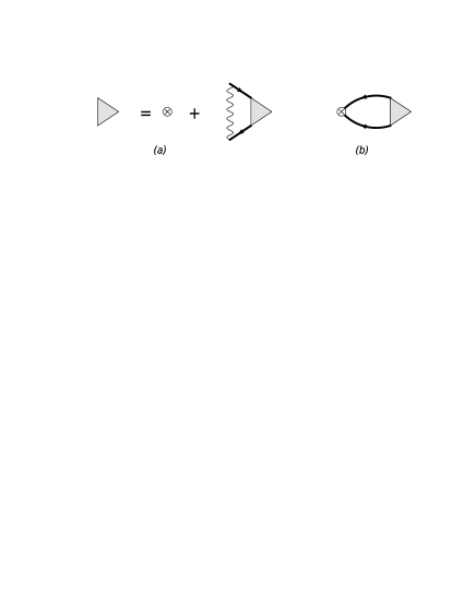
Figure 1: (a) Diagrammatic equation for the three point vertex (shaded triangle) in the ladder approximation. The cross denotes a mass vertex. (b) Response function diagram.

Denoting three-momenta $q=(q_{0},\vec{q}\,)$ one has

$$\Pi_{nm}(q)=2i\int\frac{d^{3}p}{(2\pi)^{3}}\;tr\left[M_{n}G(p)\Gamma_{m}(p,p+q)G(p+q)\right],$$ (12)

where the mass vertex $\Gamma_{m}$ is a 4x4 matrix (the sublattice/valley index is omitted for clarity), and the factor of 2 accounts for spin. In the ladder approximation $\Gamma_{m}$ satisfies the self-consistent equation

$$\Gamma_{m}(p,q)=M_{m}+ie^{2}\int\frac{d^{3}k}{(2\pi)^{2}}\frac{G(k)\Gamma_{m}(k,q)G(k+q)}{|\vec{p}-\vec{k}|},$$ (13)

where (we set $v_{F}=1$ henceforth)

$$G(k)=\frac{k_{0}+\vec{\alpha}\vec{k}}{k_{0}^{2}-\vec{k}^{2}+i\epsilon}.$$ (14)

To solve this set of equations, it is convenient to decompose $\Gamma_{m}$ in a basis of 4x4 matrices with well defined transformation properties under the SU(2) valley symmetry. Defining $\tilde{M}=\tau_{z}\sigma_{z}$, this basis may be taken as the four matrices $\tilde{M},\mathcal{I},\alpha^{i}$ which are scalars under this symmetry, and the matrices $M_{n},T_{n},\alpha^{i}T_{n}$, which transform like a spin 1/2. With this choice we express $\Gamma_{m}$ as

$$\begin{split}\Gamma_{m}&=\tilde{\Gamma}_{m}\tilde{M}+\tilde{\Gamma}^{0}_{m}\mathcal{I}+\tilde{\Gamma}^{i}_{m}\alpha^{i}\\ &+\Gamma_{nm}M_{n}+\Gamma^{0}_{nm}T_{n}+\Gamma^{i}_{nm}\alpha^{i}T_{n}\end{split}.$$ (15)

The equations are further simplified when $\Gamma^{i}_{nm}$ is expressed in terms of its longitudinal and transverse parts

$$\Gamma^{L}_{nm}=\hat{q}\cdot\vec{\Gamma}_{nm}, \Gamma^{T}_{nm}=\hat{q}\times\vec{\Gamma}_{nm},$$ (16)

where $\hat{q}=\vec{q}/q$, and a similar relation applies for $\tilde{\Gamma}^{i}_{nm}$. With the identities

$$\vec{k}\cdot\vec{\Gamma}_{nm} =\vec{k}\cdot\hat{q}\;\Gamma^{L}_{nm}-\vec{k}\times\hat{q}\;\Gamma^{T}_{nm},$$ (17)

$$\vec{k}\times\vec{\Gamma}_{nm} =\vec{k}\cdot\hat{q}\;\Gamma^{T}_{nm}+\vec{k}\times\hat{q}\;\Gamma^{L}_{nm},$$ (18)

substituting Eq. (15) into Eq. (12), and performing the trace, we obtain

$$\Pi_{nm}(q)=i\int \frac{d^{3}p}{(2\pi)^{3}}\;\frac{8}{D}\left[f_{11}\Gamma_{nm}+f_{12}\Gamma^{T}_{nm}\right.$$

$$\left.+\vec{p}\times\vec{q}(f_{13}\Gamma^{L}_{nm}+f_{14}\Gamma^{0}_{nm})\right],$$ (19)

where we have defined the denominator

$$D(p,q)=[p_{0}^{2}-\vec{p}^{2}+i\epsilon][(p_{0}+q_{0})^{2}-(\vec{p}+\vec{q})^{2}+i\epsilon],$$ (20)

and where all $f_{ij}(\vec{p},\vec{q})$ (specified below) are even functions under the reversal of the relative angle $\theta_{\vec{p},\vec{q}}=\theta_{p}-\theta_{q}$. Because of the decomposition in Eq. (15), the scalar parts decouple completely and are not needed. We can then obtain equations for the remaining components of $\Gamma_{m}$ by multiplying Eq. (13) by the corresponding basis matrices and taking the trace. One then obtains

$$\Gamma_{nm} =\delta_{nm}-i\beta\int\frac{d^{3}k}{(2\pi)^{2}}\frac{1}{D}\frac{1}{|\vec{p}-\vec{k}|}\left[f_{11}\Gamma_{nm}+f_{12}\Gamma^{T}_{nm}\right.$$

$$\left.+\vec{k}\times\vec{q}(f_{13}\Gamma^{L}_{nm}-f_{14}\Gamma^{0}_{nm})\right],$$ (21)

$$\Gamma^{T}_{nm} =-i\beta\int\frac{d^{3}k}{(2\pi)^{2}}\frac{1}{D}\frac{1}{|\vec{p}-\vec{k}|}\left[f_{21}\Gamma_{nm}+f_{22}\Gamma^{T}_{nm}\right.$$

$$\left.+\vec{k}\times\vec{q}\left(f_{23}\Gamma^{L}_{nm}+f_{24}\Gamma^{0}_{nm})\right)\right].$$ (22)

$\Gamma^{L}_{mn}$ and $\Gamma^{0}_{mn}$ satisfy similar equations, but are not needed in what follows. We now perform a circular harmonic expansion

$$\Gamma^{(n_{p},n_{q})}=\int\frac{d\theta_{p}}{2\pi}e^{in_{p}\theta_{p}}\frac{d\theta_{q}}{2\pi}e^{in_{q}\theta_{q}}\Gamma(p,q),$$ (23)

and retain only the first order contribution. Terms containing $\vec{k}\times\vec{q}$ are odd and vanish. Thus, $\Gamma^{L}_{n}$ and $\Gamma^{0}_{n}$ completely decouple to first order. Moreover, from the structure of Eqs. (III), (III) and (III) it can be seen that in fact $\Pi_{nm}=\delta_{nm}\Pi$. As expected, the Kekulé ($\Pi_{11}$ and $\Pi_{22}$) and CDW ($\Pi_{33}$) response functions are the same.

With this simplification the relevant components of $f_{ij}$ are

$$f_{11} =-k_{0}(k_{0}+q_{0})+\vec{k}(\vec{k}+\vec{q}\,),$$ (24)

$$f_{12} =f_{21}=i(\frac{q_{0}\vec{k}\vec{q}}{q}-k_{0}q),$$ (25)

$$f_{22} =\frac{2(\vec{q}\times\vec{k})^{2}}{q^{2}}+k_{0}(k_{0}+q_{0})-\vec{k}(\vec{k}+\vec{q}\,).$$ (26)

Defining the dimensionless kernels

$$K_{ij}^{(n)}=\frac{i}{\pi}\int\frac{d\theta_{p}}{2\pi}e^{\theta_{p}n}\int dk_{0}k\frac{f_{ij}}{D},$$ (27)

and

$$C^{(n)}(x)=\int\frac{d\theta_{k}}{2\pi}\frac{e^{in\theta_{k}}}{(1+x^{2}+2x\cos\theta_{k})^{1/2}},$$ (28)

the self-consistent equations to first order in the circular harmonic expansion finally read

$$\Gamma^{(0,0)}=1+\frac{\beta}{2p}\int dkC^{(0)}(K_{11}^{(0)}\Gamma^{(0,0)}+K_{12}^{(0)}\Gamma_{T}^{(0,0)}),$$ (29)

$$\Gamma_{T}^{(0,0)}=-\frac{\beta}{2p}\int dkC^{(0)}(K_{21}^{(0)}\Gamma^{(0,0)}+K_{22}^{(0)}\Gamma_{T}^{(0,0)}).$$ (30)

A numerical analysis shows that the mixing kernel $K_{12}$ is small compared to $K_{11}$ and may be neglected also. In this case, the final equations determining the response function, spelling all momentum dependence, read

$$\Gamma^{(0,0)}(p,q) =1+\frac{\beta}{2p}\int_{0}^{\Lambda}dkC^{(0)}(k/p)K_{11}^{(0)}(k,q)\Gamma^{(0,0)}(k,q),$$ (31)

$$\Pi(q) =\frac{2}{\pi}\int_{0}^{\Lambda}dpK_{11}^{(0)}(p,q)\Gamma^{(0,0)}(p,q),$$ (32)

where $\Lambda$ is an ultraviolet cutoff regularizing the integrals. Note the product $C^{(0)}(k/p)K_{11}^{(0)}(k,q)$ goes as $p/k$ for large $k$, so the iteration of this equation produces a series of logarithms characteristic of power law behaviour. Also note that when the external $q<q_{0}$, all $K_{ij}$ develop an imaginary part for $(q_{0}-q)/2<k<(q_{0}+q)/2$.

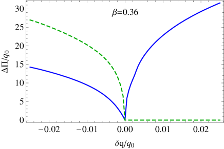
Figure 2: Mass susceptibility $\Delta\Pi(q_{0},q_{0}+\delta q)$ for $|\delta q|<<q_{K}$ and $\beta=0.36$, real part (full line) and imaginary part (dashed line).

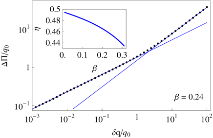
Figure 3: Logarithmic plot of the mass susceptibility $\Delta\Pi(q_{0},q_{0}+\delta q)$ for $\beta=0.24$ and $\delta q>0$ (dotted line). The full lines are linear fits with $\eta=0.45$ for $\delta q<<q_{K}$ and $\eta_{0}=0.69$ for $\delta q>>q_{K}$. Inset: The exponent $\eta$ as a function of $\beta$.

We solve Eq. (31) numerically by discretizing the momentum $k$ on a logarithmic mesh and solving the corresponding matrix equation by Gaussian elimination. The integration of Eq. (32) is straightforward. The result of this procedure is $\Pi(q_{0},q)$. It is convenient to represent it as the difference $\Delta\Pi=\Pi(q_{0},q_{0}+\delta q)-\Pi(q_{0},q_{0})$ with $\delta q=q_{0}-q$. Fig. 2 displays the real and imaginary parts of $\Delta\Pi$ for $|\delta q|<<q_{0}$. We observe a cusp at $\delta q=0$ in the real part, and a finite imaginary part for $\delta q<0$. Log plots of both sides of the real part and and the imaginary part reveal power laws as $\delta q\rightarrow 0$. A Kramers-Kronig analysis for $|\delta q|<<q_{0}$ shows that this is only consistent if $\Delta\Pi\propto(\delta q)^{\eta}$, i.e. the exponents are all the same. Fig. 3 shows a log plot for $\delta q>0$ where power law behavior is evident for $\delta q<<q_{0}$. We also observe that $\Delta\Pi$ crosses over to a different power law for $\delta q>>q_{0}$, which we identify as the static result $q^{\eta_{0}}$ WFM10 . The inset of Fig. 3 shows that $\eta$ is $\beta$-dependent, and that it tends to the non-interacting result in Eq. (10) as $\beta\rightarrow 0$. The dependence of $\eta_{0}$ on $\beta$ can be found in Ref. WFM10, .

Finally, we plot the phonon dispersion relation, which is the main result of this work. This is given in terms of the self-energy evaluated at the phonon frequency $\omega_{K}$. To ease the comparison at different values of $\beta$, we will also represent the difference

$$\Delta\omega(q)=\omega(q)-\omega(q_{K})=\frac{\lambda_{K}}{2}\left(\Pi(\omega_{K},q)-\Pi(\omega_{K},q_{K})\right)$$ (33)

where we have recovered physical units with $\hbar v_{F}=6.5$ eV$\AA$. The values of the parameters used are $\lambda_{K}=0.1$ and $\Lambda=1.7eV$. The phonon dispersion is depicted in Fig. 4 for different values of $\beta$. The dispersion follows the static power law $q^{\eta_{0}(\beta)}$ for $q>>q_{K}$, and the cusp turns into $q^{\eta(\beta)}$ as discussed.

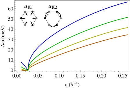
Figure 4: $A_{1}$ phonon dispersion relation $\Delta\omega(q)$ measured from the K point for $\beta=0,0.1,0.2,0.3$, with higher curves corresponding to higher values of $\beta$. Note that $\omega(q_{K})$, which depends on $\beta$, has been substracted from each curve for an easier comparison. Inset: the Kekulé phonon displacements.

IV Discussion

Our computation has shown that interactions turn the Kohn anomaly at the K point into a power law, so it is natural to ask whether the same effect happens for the anomaly at $\Gamma$. This is not expected in general grounds, because the corresponding self-energy is built with vertices corresponding to a conserved current, and these type of operators do not have anomalous dimensions because of Ward identities FPS03 . This is also consistent with the fact that the Coulomb interaction renormalizes the $A_{1}$ electron-phonon coupling strongly, but not the $E_{2}$ one BA08 ; LAW08 . Power law behavior is thus only expected in the $K$ point anomaly.

From the experimental point of view, there are several techniques available for the measurement of the $A_{1}$ phonon dispersion, and each one has its own potential difficulties. In general, the power law at $q>q_{K}$ appears in a range of momenta that has been already probed with different techniques, while the cusp structure lies within the precision limits of current experiments, and may require more effort.

Electron Energy Loss Spectroscopy (EELS) is for example a suitable technique that has already been used to map the phonon dispersion at the K-point in graphene. This experiments have been performed on different substrates for which graphene behaves as quasi-freestandingYTI05 ; PMF11 , such as Pt (this is important as hybridization with the substrate strongly changes the electron band structure and the Kohn anomaly AW10 ). Metallic screening is however a disadvantage as it spoils the critical behaviour of the electrons, and an insulating substrate would be more suited to observe the effect.

A more indirect experiment (with insulating substrate) is to track the dependence of the 2D Raman peak with incoming laser energy. This method has been used MSM07 to measure the dispersion of the $A_{1}$ phonon. While the amount of data it yields and the range of momenta it covers is limited and not very close to the $K$ point, the observation of the $q>q_{k}$ regime is certainly possible. Finally, X-rays are a usual tool to measure phonon dispersions in 3D crystals, and while it is probably challenging to obtain enough intensity from a single sheet of graphene, experiments in graphite MET04 ; GSB09 might be used to deduce the phonon dispersion. This approach is not straightforward because the electronic structure of graphite is different from graphene, and this must be taken into account. Nevertheless, it is encouraging to observe that precision measurements show an $A_{1}$ phonon dispersion that is not at all linear GSB09 .

A final comment concerns the robustness of our result to more refined approximations schemes than the ladder summation. While other sets of diagrams may modify our quantitative predictions, it is very unlikely that the non-analytic behaviour can be removed in this way. One may consider, for example, the inclusion of self-energy terms for the electron propagator GGV94 , which may produce a slow logarithmic dependence of the exponent. Finally, we also note that the 1/N approximation does gives power law behaviour for the Kekulé mass correlator G10 ; GMP10 (and thus the self-energy) as well.

In summary, this work has shown that the elusive critical behavior of interacting Dirac electrons in graphene manifests itself through a power law Kohn anomaly for the $A_{1}$ phonon at the K point.

V Acknowledgments

We thank A. Politano for very useful discussions. Support from NSF through Grant No. DMR-1005035, and from US-Israel Binational Science Foundation (BSF) through Grant No. 2008256 is acknowledged.

References

- (1) A. H. Castro Neto, F. Guinea, N. M. R. Peres, K. S. Novoselov, and A. K. Geim, Rev. Mod. Phys. 81, 109 (2009)
- (2) V. N. Kotov, B. Uchoa, V. M. Pereira, A. H. Castro Neto, and F. Guinea, Rev. Mod. Phys., submitted
- (3) J. González, F. Guinea, and M. A. H. Vozmediano, Nucl. Phys. B 424, 595 (1994)
- (4) D. E. Sheehy and J. Schmalian, Phys. Rev. Lett. 99, 226803 (2007)
- (5) D. V. Khveshchenko, Phys. Rev. Lett. 87, 246802 (2001)
- (6) O. V. Gamayun, E. V. Gorbar, and V. P. Gusynin, Phys. Rev. B 81, 075429 (2010)
- (7) J. P. Reed, B. Uchoa, Y. I. Joe, Y. Gan, D. Casa, E. Fradkin, and P. Abbamonte, Science 330, 805 (2010)
- (8) D. C. Elias, R. V. Gorbachev, A. S. Mayorov, S. V. Morozov, A. A. Zhukov, P. Blake, L. A. Ponomarenko, I. V. Grigorieva, K. S. Novoselov, F. Guinea, and A. K. Geim, Nat. Phys.(2011)
- (9) J. Wang, H. A. Fertig, and G. Murthy, Phys. Rev. Lett. 104, 186401 (2010)
- (10) J. González, Phys. Rev. B 82, 155404 (2010)
- (11) A. Giuliani, V. Mastropietro, and M. Porta, Phys. Rev. B 82, 121418 (2010)
- (12) M. Franz, T. Pereg-Barnea, D. E. Sheehy, and Z. Tešanović, Phys. Rev. B 68, 024508 (2003)
- (13) V. P. Gusynin, D. V. Khveshchenko, and M. Reenders, Phys. Rev. B 67, 115201 (2003)
- (14) D. L. Mafra, G. Samsonidze, L. M. Malard, D. C. Elias, J. C. Brant, F. Plentz, E. S. Alves, and M. A. Pimenta, Phys. Rev. B 76, 233407 (2007)
- (15) A. Grüneis, J. Serrano, A. Bosak, M. Lazzeri, S. L. Molodtsov, L. Wirtz, C. Attaccalite, M. Krisch, A. Rubio, F. Mauri, and T. Pichler, Phys. Rev. B 80, 085423 (2009)
- (16) A. Politano, A. R. Marino, V. Formoso, and G. Chiarello, Carbon 50, 734 (2012)
- (17) A. Luther and I. Peschel, Phys. Rev. B 9, 2911 (1974)
- (18) C. Chamon, Phys. Rev. B 62, 2806 (2000)
- (19) H. Suzuura and T. Ando, J. Phys. Soc. Jpn. 77, 044703 (2008)
- (20) A. C. Ferrari, J. C. Meyer, V. Scardaci, C. Casiraghi, M. Lazzeri, F. Mauri, S. Piscanec, D. Jiang, K. S. Novoselov, S. Roth, and A. K. Geim, Phys. Rev. Lett. 97, 187401 (2006)
- (21) M. Lazzeri, C. Attaccalite, L. Wirtz, and F. Mauri, Phys. Rev. B 78, 081406 (2008)
- (22) S. Viola Kusminskiy, D. K. Campbell, and A. H. Castro Neto, Phys. Rev. B 80, 035401 (2009)
- (23) D. M. Basko and I. L. Aleiner, Phys. Rev. B 77, 041409 (2008)
- (24) D. M. Basko, S. Piscanec, and A. C. Ferrari, Phys. Rev. B 80, 165413 (2009)
- (25) S. Piscanec, M. Lazzeri, F. Mauri, A. C. Ferrari, and J. Robertson, Phys. Rev. Lett. 93, 185503 (2004)
- (26) M. Lazzeri and F. Mauri, Phys. Rev. Lett. 97, 266407 (2006)
- (27) A. H. Castro Neto and F. Guinea, Phys. Rev. B 75, 045404 (2007)
- (28) W.-K. Tse, B. Y.-K. Hu, and S. Das Sarma, Phys. Rev. Lett. 101, 066401 (2008)
- (29) S. Pisana, M. Lazzeri, C. Casiraghi, K. S. Novoselov, A. K. Geim, A. C. Ferrari, and F. Mauri, Nat. Mater. 6, 198 (2007)
- (30) H. Yanagisawa, T. Tanaka, Y. Ishida, M. Matsue, E. Rokuta, S. Otani, and C. Oshima, Surface and Interface Analysis 37, 133 (2005)
- (31) A. Allard and L. Wirtz, Nano Letters 10, 4335 (2010)
- (32) J. Maultzsch, S. Reich, C. Thomsen, H. Requardt, and P. Ordejón, Phys. Rev. Lett. 92, 075501 (2004)