Exclusive diffractive production of real photons and vector mesons in a factorized Regge-pole model with non-linear Pomeron trajectory

Abstract

Exclusive diffractive production of real photons and vector mesons in ep collisions has been studied at HERA in a wide kinematic range. Here we present and discuss a Regge-type model of real photon production (Deeply Virtual Compton Scattering), as well as production of vector mesons (VMP) treated on the same footing by using an extension of a factorized Regge-pole model proposed earlier. The model has been fitted to the HERA data. Despite the very small number of the free parameters, the model gives a satisfactory description of the experimental data, both for the total cross section as a function of the photon virtuality $Q^{2}$ or the energy $W$ in the center of mass of the $\gamma^{*}p$ system, and the differential cross sections as a function of the squared four-momentum transfer $t$ with fixed $Q^{2}$ and $W$.

I Introduction

Measurements of exclusive deep inelastic processes, such as the production of a real photon or a vector meson, processes known as Deeply Virtual Compton Scattering (DVCS) and Vector Meson Production (VMP), respectively, opened a new window in the study of the nucleon structure in three dimensions, namely in the virtuality $Q^{2}$, the energy $W$ in the center of mass of the $\gamma^{*}p$ system and the squared momentum transfer $t$. The construction of scattering amplitudes depending simultaneously on these variables is a challenge for the theory and its knowledge is necessary for the deconvolution of the relevant Generalized Parton Distributions (GPDs). These ones provide information on parton distributions in the coordinate space and, in a more restricted sense, the parton density in the 2D impact parameter space. They are complementary to the linear momentum distribution in the variable $x$ to give a tomographic picture of the nucleon.

The aim of the present paper is to construct an explicit model for the DVCS and VMP amplitudes depending on the three independent variables $Q^{2}$, $W$ and $t$. The amplitude should satisfy Regge behaviour, scaling behaviour, be compatible with the quark counting rules and fit the experimental data on DVCS and VMP. In this paper we extend a model on DVCS DVCS , published earlier by some of the authors, to include VMP. Besides the similarities between these two processes, there are also differences. In a number of papers, Regge-pole models were successfully applied to VMP (for a review on VMP at HERA see Ref. Nikolaev ). The main problem is how the photon virtuality $Q^{2}$ enters the scattering amplitude. In Ref. Schild , the $Q^{2}$ dependence is described via a generalization of the vector dominance model. According to Donnachie and Landshoff L ; DL , the $Q^{2}$ evolution can be effectively mimicked by a properly chosen factor in front of the Regge-pole terms. Moreover the same authors argue that HERA data on DVCS and VMP indicate the existence of a soft and a hard Pomeron, whose relative contribution changes with the hardness of the reaction, i.e. with the photon virtuality and the mass of produced vector mesons.

The paper is organized as follows. In Section II we remind the main features of the model. In Section III we illustrate our fitting strategy and present the results of fits of our model to experimental data on DVCS and VMP processes. In Section IV there are our conclusions. Details of the calculation of the integrated cross section with a non-linear Pomeron trajectory are given in the Appendix.

II The Model

II.1 Kinematics

The diagrams of the reactions in question, DVCS and VMP processes, with a single-photon exchange, are shown in Fig. 1. Since we are interested in the nucleon structure, the precisely calculable electroweak vertex $e^{-}\gamma e^{-}$ of Fig. 1(a,b) can be factorized out. In the remaining sub-process $\gamma^{*}p\rightarrow\gamma(V)p$, where $\gamma^{*}$ is the incoming virtual photon and the outgoing vector particle is a real photon $\gamma$ (Fig. 1 (a)) or a vector meson V (Fig. 1(b)), at high energies, typical of the HERA experiments, the amplitude is dominated by Regge exchanges, as shown in Fig. 1(c). In the center of mass of the $\gamma^{*}p$ system the three independent variables of the reactions are, as said above, the virtuality $Q^{2}=-q_{1}^{2}$, whose physical values are positive, the energy $W=(p_{1}+q_{1})$ and squared momentum transfer $t=(q_{2}-q_{1})^{2}$. In the study of VMP it is customary to combine the virtuality $Q^{2}$ and the squared mass of the produced vector particle $M^{2}_{V}$ as $\tilde{Q}^{2}=Q^{2}+M_{V}^{2}$. Note that there is no proof for this relation, it is rather a plausible assumption. Moreover, a weight factor might enter the game, namely we could perform the substitution $\tilde{Q}^{2}\Rightarrow c\cdot\tilde{Q}^{2}$.

In Ref. DVCS one further step was made, introducing a new variable $z$ through the combination

$$z=t-Q^{2}.$$ (1)

The argument in favor of this relation is that both $t$ and $-Q^{2}$ have the meaning of the squared momentum transfer and are an indication of the softness - hardness of the dynamics.

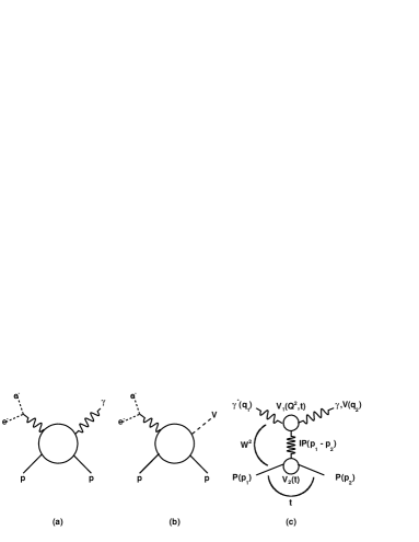
Figure 1: Diagrams of DVCS (a) and VMP (b); (c) DVCS (VMP) amplitude in a Regge-factorized form.

II.2 The Amplitude

In Ref. DVCS a simple factorized Regge-pole model for DVCS was suggested and successfully fitted to the HERA data. Here we extend the analysis to VMP processes by using the main ideas of the model. The extension includes a more detailed analysis of the $Q^{2}$ and $M_{V}^{2}$ dependence on dynamics. Note that at the HERA energies sub-leading (secondary Reggeon) contributions are negligible, so that a Pomeron exchange can account for the whole dynamics of the reaction. The Pomeron pole contribution was defined in Ref. DVCS on the following grounds:

• it is a single and factorable Regge pole;

• the dependence on the mass and virtuality of the external particles enters via the relevant residue functions, which means that the virtuality $Q^{2}$ and the produced vector meson mass enter only via the upper residue on Fig. 1(c), $V_{1}$, while the Pomeron trajectory $\alpha(t)$ is universal and $Q^{2}$-independent;

• following dual models (see, for instance, Ref. BGJPP ), we introduce a $t$ dependence in the residues that enters solely in terms of the trajectory;

• the Pomeron trajectory has the form

  $$\alpha(t)=\alpha_{0}-\alpha_{1}\ln(1-\alpha_{2}t),$$ (2)

  where $\alpha_{i},\ \ i=0-2$, are the $\alpha(t)$-trajectory parameters. This choice is unique for the trajectory, giving a nearly linear behaviour at small $|t|$, where $\alpha^{\prime}=\alpha_{1}\alpha_{2}$ is the forward slope, whereas at large $|t|$ the amplitude and the cross section obey scaling behaviour governed by the quark counting rule. In fact, the logarithmic asymptotics of the trajectory is required by the scaling of the fixed angle scattering amplitude (see Refs. FJMP ; DVCS , moreover it follows from perturbative Quantum Chromodynamic (pQCD) calculations (consider, for instance, the BFKL theory BFKL ).

Fig. 2 shows the comparison of our logarithmic trajectory with a linear one, $\alpha_{0}+\alpha^{\prime}t$, where $\alpha_{0}=1.09$ and $\alpha^{\prime}=0.25$ GeV^-2 for the intercept and the slope respectively, typical of the soft processes L , have been used. The logarithmic asymptotics are important for physical reasons: at large $|t|$ the amplitude and the cross sections obey scaling behaviour governed by the quark counting rules, as seen in hadronic reactions FJMP , where sufficiently large values of $|t|$ have been reached in $pp$ and $\bar{p}p$ scattering, confirming the quark counting rules. More arguments in favour of the logarithmic behaviour in $Q^{2}$ can be found in Ref. a . This is expected in future measurements  Boeretal , and should be implied, in DVCS and VMP as well. The high $Q^{2}$ region is governed by QCD evolution, and it is beyond the scope of the Regge-pole models. In any case, according to the DGLAP evolution equation DGLAP , the high $Q^{2}$ behaviour must be tempered with respect to that given by the linear trajectory, and be closer to the logarithmic one, or maybe even slower (double logarithmic?). This behaviour was studied in Ref. CJKLMP .

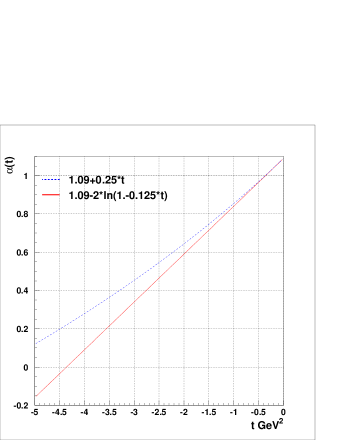
Figure 2: Logarithmic vs linear trajectory as function of t.

Neglecting spin, the invariant scattering amplitude with a simple Regge pole exchange, as shown in Fig. 1(c), can be written as

$$A(s,t,\tilde{Q}^{2})_{\gamma^{*}p\rightarrow\gamma(V)p}=-A_{0}V_{1}(t,\tilde{Q}^{2})V_{2}(t)(-is/s_{0})^{\alpha(t)}.$$ (3)

Here $A_{0}$ is a normalization factor, $V_{1}(t,\tilde{Q}^{2})=$ exp$[b_{2}\beta(z)]$ is the $\gamma^{*}I\!\!P\gamma$ vertex, $V_{2}(t)=$ exp$[b_{1}\alpha(t)]$ is the $pI\!\!Pp$ vertex, being $\beta(z)$ and $\alpha(t)$ the exchanged Pomeron trajectory in the photon vertex and in the proton vertex, respectively.

Similarly to Ref. Mullerfit , in Ref. DVCS for DVCS only the helicity conserving amplitude was considered. For not too large $Q^{2}$ the contribution from longitudinal photons is small (it vanishes for $Q^{2}=0$). Moreover, at high energies, typical of the HERA collider, the amplitude is dominated by the helicity conserving Pomeron exchange and, since the final photon is real and transverse, the initial one is also transverse. Electroproduction of vector mesons, discussed in the present paper, requires to take into account both the longitudinal and transverse cross sections. For convenience, and following the arguments based on duality (see Ref. DVCS and references therein), the $t$ dependence of the $pI\!\!Pp$ vertex $V_{2}$ is introduced via the trajectory and a generalization of this concept is applied also to the $\gamma^{*}I\!\!P\gamma$ vertex $V_{1}$, which however, apart from $t$, depends also on $Q^{2}$ through the trajectory

$$\beta(z)=\beta_{0}-\beta_{1}\ln(1-\beta_{2}z),$$ (4)

where $\beta_{i},\ \ i=0-2$, are the $\beta(z)$-trajectory parameters, and $\beta_{1}\beta_{2}=\beta^{\prime}$ is the forward slope of this trajectory.

Hence the scattering amplitude in Eq. (3) can be written in the form

$$A(s,t,\tilde{Q}^{2})_{\gamma^{*}p\rightarrow\gamma(V)p}=-A_{0}e^{b_{2}\beta(z)}e^{b_{1}\alpha(t)}(-is/s_{0})^{\alpha(t)}.$$ (5)

Although the model has many parameters, most of them are constrained by plausible assumptions. First, we fix the intercepts of both $\alpha(t)$ and $\beta(z)$ to the value of $1.09$. The Hardening of the dynamics with increasing $\tilde{Q}^{2}$ may be accounting for either by letting the intercept to be $\tilde{Q}^{2}$-dependent, unacceptable by Regge-factorization, or by introducing one more, hard component in the Pomeron (still unique!) with a $\tilde{Q}^{2}$-dependent residue, as suggested e.g. in Refs. DL and FFJL . In any case, the trajectories and their parameters are the same for DVCS and for VMP. The other two parameters of the trajectories, $\alpha_{1}$ and $\alpha_{2}$ ($\beta_{1}$ and $\beta_{2}$) are fixed in the following way: their product $\alpha^{\prime}=\alpha_{1}\alpha_{2}$ ($\beta^{\prime}=\beta_{1}\beta_{2}$) is their forward slope, that we set equal to the value $\alpha^{\prime}=0.25$ GeV^-2. Furthermore, since $\alpha_{1}\approx 2$ from the quark counting rules (see Ref. DVCS ), we get $\alpha_{2}=\alpha^{\prime}/\alpha_{1}=0.125$ GeV^-2. The same values are used also for the correspondent $\beta_{1}$ $\beta_{2}$ parameters of the $\beta(z)$-trajectory.

The parameter $s_{0}$ is not fixed by the Regge-pole theory. The nice and plausible relation $s_{0}=1/\alpha^{\prime}\approx(1/4)m^{2}_{p}$ follows from the hadronic string model BaPre , other values, however, cannot be excluded. We set, for sake of simplicity, $s_{0}=m^{2}_{p}\approx 1$ GeV².

Finally, we set the parameter $b_{1}$ entering the proton vertex (lower vertex of Fig. 1(c)) to $b_{1}=2.0$. In fact, this (p$I\!\!P$p) vertex is know from the analysis of the $pp$ and $\bar{p}p$ scattering to be of the form exp$(bt)$, and an estimate of $b$ is $b\approx 2$ GeV^-2 (see for this Ref. b and references therein).

In Table 1 we summarize the values of all parameters fixed following the arguments above. Thus, the only free parameters we remain with are the parameter $b_{2}$, entering the photon vertex $\gamma^{*}I\!\!P\gamma(V)$, and the squared modulus of the normalization factor, $|A_{0}|^{2}$.

Table 1: Values of fixed parameters of our model.

$\alpha_{0}=\beta_{0}$	$\alpha_{1}=\beta_{1}$	$\alpha_{2}=\beta_{2}~{}[GeV^{-2}]$	$s_{0}~{}[GeV^{2}]$	$b_{1}$	$\alpha^{\prime}=\beta^{\prime}~{}[GeV^{-2}]$	$M^{2}_{V}~{}[GeV^{2}]$
1.09	2.00	0.125	1.00	2.00	0.25	$M^{2}_{\gamma}=0$; $M^{2}_{\rho,\phi,...}$;

II.3 Cross Sections

Having fixed most of the parameters of the model as explained above, from the amplitude (5) we can now construct the physical quantities to be fitted to the experimental data.

Notice that in this amplitude there is no room for sub-leading trajectories (e.g. the $f$-trajectory) contribution, because they are suppressed at the Hera energies DL . This assumption has been confirmed by an exploratory fit with an amplitude containing also an $f$-Reggeon contribution ($\alpha_{0}=0.5$ and $\alpha^{\prime}=1~{}$GeV^-2). We found that the $f$-Reggeon contribution is totally negligible.

The differential cross-section $d\sigma(\gamma^{*}~{}p\rightarrow\gamma(V)~{}p)/dt$ is defined as

$${d\sigma\over{dt}}(\tilde{Q}^{2},W,t)={\pi\over{s^{2}}}|A(\tilde{Q}^{2},W,t)|^{2}.$$ (6)

The slope of the differential cross section as a function of t is given by

$$B(\tilde{Q}^{2},W,t)={d\over{dt}}\ln|A(\tilde{Q}^{2},W,t)|^{2}.$$ (7)

The total cross section can be approximated as follows:

$$\sigma(s,\tilde{Q}^{2}) = \int_{t_{min}\approx-s/2}^{t_{threshold}\approx-4m^{2}_{p}}dt{d\sigma(s,t,\tilde{Q}^{2})\over{dt}}$$ (8)

$$\approx \left[{1\over B(s,t,\tilde{Q}^{2})}{d\sigma(s,t,\tilde{Q}^{2})\over{dt}}\right]_{t=0}$$

$$= \frac{|A_{0}|^{2}\pi e^{2\alpha_{0}(b_{1}+b_{2})}}{[b_{1}+\ln(s/s_{0})](1+\alpha_{2}\tilde{Q}^{2})+b_{2}}\cdot$$

$$\cdot\frac{(s/s_{0})^{2\alpha_{0}}}{2\alpha^{\prime}s^{2}(1+\alpha_{2}\tilde{Q}^{2})^{2b_{2}\alpha_{1}-1}}.$$

Expression (8) was obtained in the limit $s\rightarrow\infty$. Alternatively, the integral can be analytically calculated; this is done in Appendix and the result is (see Eq. (15))

$$\sigma(s,\tilde{Q}^{2})=\frac{K}{\mu-1}~{}{{}_{2}}F_{1}\left(2b_{2}\alpha_{1},\mu-1;\mu;-\alpha_{2}\tilde{Q}^{2}\right),$$ (9)

where

$$K = \frac{\pi|A_{0}|^{2}}{\alpha_{2}~{}s^{2}}e^{2\alpha_{0}(b_{1}+b_{2})}(s/s_{0})^{2\alpha_{0}},$$ (10)

$$\mu = 2\alpha_{1}\left[b_{1}+b_{2}+\ln(s/s_{0})\right].$$ (11)

Performing an exploratory fit both expressions for the total cross sections lead to results consistent with each other. This means that the main contribution to the total cross section comes from the region close to $t=0$. We decided to use the exact analytical expression in the fit procedure.

III Fitting Strategy and Results

In the present paper the differential and the total cross sections have been fitted to the HERA data on DVCS d1 ; d2 ; d3 ; d4 and electroproduction of vector mesons $\rho^{0}$ r1 ; r2 , $\phi$ r1 ; phi_zeus , $\omega$ omega_zeus and $J/\Psi$ j1 ; j2 . The fit on $\sigma(\tilde{Q}^{2})$ is the most sensitive to the parameter $b_{2}$ and gives a precise estimation of it. For these reason we first performed preliminary fits of the total cross section as a function of $\tilde{Q}^{2}$ at fixed $W$, to HERA data on DVCS and VMP collected by the H1 and ZEUS Collaborations, in order to get weighted average values for $b_{2}$. Then, keeping $b_{2}$ fixed to these average values, we performed one-parameter fits to the data for $\sigma(Q^{2})$, $\sigma(W)$ and $d\sigma/dt$, the only free parameter being the normalization $A_{0}$.

III.1 DVCS

Experimental data for the fits are taken from Refs. d1 ; d2 ; d3 ; d4 . The exploratory fit to determine the weighted average value of $b_{2}$ gives globally a rather satisfactory result, which is shown in Table 2. Here and in the following Tables $\tilde{\chi}^{2}$ means $\chi^{2}$/d.o.f.

Table 2: Values of the two free parameters $|A_{0}|$, $b_{2}$ and $\tilde{\chi}^{2}$, from the two-parameter fit of the total cross section to data from Refs. d1 ; d3 ; d4 of $\gamma^{*}p\rightarrow\gamma p$ as function of $Q^{2}$ and fixed $W$. The average value of $b_{2}$ was found to be: $<b_{2}>=0.690\pm 0.021$

	$\sigma_{(\gamma^{*}~{}p~{}->~{}\gamma~{}p)}(Q^{2})$
Coll.	Years	$W$ [GeV]	$|A_{0}|$ [nb]1/2	$b_{2}$	$\tilde{\chi}^{2}$
H1	04-07	82	0.164 $\pm$ 0.012	0.641 $\pm$ 0.055	1.1
H1	96-00	82	0.162 $\pm$ 0.011	0.656 $\pm$ 0.069	0.7
ZEUS$(e^{-})$	96-00	89	0.177 $\pm$ 0.013	0.703 $\pm$ 0.091	0.6
ZEUS$(e^{+})$	96-00	89	0.170 $\pm$ 0.005	0.596 $\pm$ 0.026	0.4
ZEUS	99-00	104	0.209 $\pm$ 0.010	0.769 $\pm$ 0.077	3.3

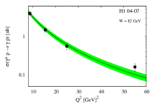
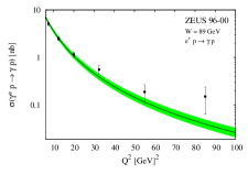
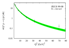
Figure 3: The behaviour according to our model of $\gamma^{*}p\rightarrow\gamma p$ total cross section as function of $Q^{2}$ is compared with data from Refs. d1 ; d3 ; d4 measured by the H1 and ZEUS Collaborations for several values of $W$. The green bands are calculated accordingly with the uncertainties on the free parameter $|A_{0}|$.

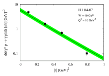
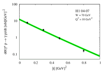
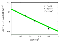
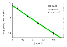
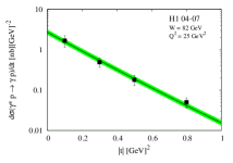
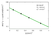
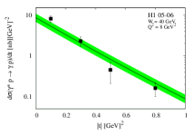
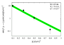
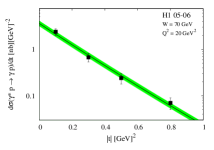
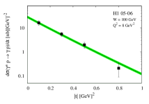
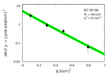
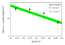
Figure 5: The behaviour according to our model of $\gamma^{*}p\rightarrow\gamma p$ differential cross section as function of $t$ is compared with data from Refs. d2 ; d3 ; d4 measured by the H1 and ZEUS Collaborations for several values of $Q^{2}$ and $W$. The green bands are calculated accordingly with the uncertainties on the free parameter $|A_{0}|$.

Having fixed the parameter $b_{2}$ to the weighted average value 0.690(21), all subsequent fits are performed with only $|A_{0}|$ as free parameter. In Figs. 3, 4 and Tables 3, 4 we present the result for the total cross section as a function of $Q^{2}$ at fixed $W$ and as a function of $W$ at fixed $Q^{2}$, respectively, while in Fig. 5 and Table 5 we present the results for the differential cross section. The result appears fairly good, except for high value of $Q^{2}$, for which we can observe some discrepancy between experimental data and our description.

Table 3: Values of the free parameter $|A_{0}|$ and $\tilde{\chi}^{2}$ from the fit to data from Refs. d1 ; d3 ; d4 of $\gamma^{*}p\rightarrow\gamma p$ total cross section as function of $Q^{2}$ for fixed values of $W$ and of $<b_{2}>=0.690\pm 0.021$.

	$\sigma_{(\gamma^{*}~{}p~{}->~{}\gamma~{}p)}(Q^{2})$
Coll.	Years	$W$ [GeV]	$|A_{0}|$ [nb]1/2	$\tilde{\chi}^{2}$
H1	04-07	82	0.172 $\pm$ 0.006	1.0
H1	96-00	82	0.165 $\pm$ 0.008	0.6
ZEUS$(e^{-})$	96-00	89	0.176 $\pm$ 0.006	0.4
ZEUS$(e^{+})$	96-00	89	0.183 $\pm$ 0.005	1.1
ZEUS	99-00	104	0.204 $\pm$ 0.009	3.3

Table 4: Values of the free parameter $|A_{0}|$ and $\tilde{\chi}^{2}$ from the fit to data from Refs. d1 ; d2 ; d4 of $\gamma^{*}p\rightarrow\gamma p$ integrated cross section as function of $W$ for fixed values of $Q^{2}$.

	$\sigma_{(\gamma^{*}~{}p~{}->~{}\gamma~{}p)}(W)$
Coll.	Years	$Q^{2}$ [GeV2]	$|A_{0}|$ [nb]1/2	$\tilde{\chi}^{2}$
H1	05-06	8	0.163 $\pm$ 0.008	6.0
ZEUS	99-00	2.4	0.240 $\pm$ 0.008	1.7
ZEUS	99-00	3.2	0.222 $\pm$ 0.007	3.8
ZEUS	96-00	6.2	0.181 $\pm$ 0.007	1.0
ZEUS	96-00	9.6	0.173 $\pm$ 0.007	3.2
ZEUS	96-00	9.9	0.170 $\pm$ 0.010	2.9
ZEUS	96-00	18.0	0.182 $\pm$ 0.010	1.9

Table 5: Values of the free parameter $|A_{0}|$ and $\tilde{\chi}^{2}$ from the fit to data from Ref. d3 of $\gamma^{*}~{}p\rightarrow\gamma p$ differential cross section as function of t for fixed values of Q² and W.

	$\sigma_{(\gamma^{*}~{}p~{}->~{}\gamma~{}p)}(t)$
Coll.	Years	$W$ [GeV]	$Q^{2}$ [GeV2]	$|A_{0}|$ [nb]1/2	$\tilde{\chi}^{2}$
H1	04-07	40	10	0.122 $\pm$ 0.007	1.5
H1	04-07	70	10	0.157 $\pm$ 0.003	0.3
H1	04-07	82	8	0.168 $\pm$ 0.006	0.8
H1	04-07	82	15.5	0.161 $\pm$ 0.004	0.3
H1	04-07	82	25	0.163 $\pm$ 0.008	0.4
H1	04-07	100	10	0.185 $\pm$ 0.003	0.2
H1	05-06	40	8	0.118 $\pm$ 0.0128	2.2
H1	05-06	40	20	0.109 $\pm$ 0.005	0.3
H1	05-06	70	8	0.146 $\pm$ 0.012	1.8
H1	05-06	70	20	0.150 $\pm$ 0.005	0.4
H1	05-06	100	8	0.181 $\pm$ 0.008	0.5
H1	05-06	100	20	0.171 $\pm$ 0.008	0.4
ZEUS	99-00	104	3.2	0.204 $\pm$ 0.018	0.9

III.2 Exclusive VM electroproduction ($\gamma^{*}~{}p\rightarrow V~{}p$)

To describe vector meson production (VMP) we used the same model as for DVCS. We considered exclusive electroproduction of $\rho^{0}$, $\phi$, $\omega$ and $J/\Psi$ mesons. In VMP, contrary to DVCS, apart from transversely polarized photon amplitude, the longitudinal component is also important. We have performed a fit for each reaction separately, applying the same strategy as in DVCS, using the same set of fixed parameters. First, leaving as free parameters the normalization $|A_{0}|$ and $b_{2}$, through a preliminary fit we have determined the weighted average value of the parameter $b_{2}$ for each process. Then we have fitted our model to the data having only $|A_{0}|$ as free parameter to be determined by the fit. From the results one can see how the weighted average value of the parameter $b_{2}$ of the Regge-pole in the $\gamma^{*}I\!\!P\gamma$ vertex obviously depends on the specific reaction.

III.2.1 $\gamma^{*}~{}p~{}\rightarrow~{}\rho^{0}~{}p$

Experimental data for the fits are taken from Refs. r1 ; r2 . The exploratory fit to determine the weighted average value of $b_{2}$ is shown in Table 6.

Table 6: Values of the two free parameters $|A_{0}|$, $b_{2}$ and $\tilde{\chi}^{2}$, from the two-parameter fit to data from Refs. r1 ; r2 of total cross section of $\gamma^{*}p\rightarrow\rho^{0}p$ as function of $Q^{2}$ and fixed $W$. The average value of $b_{2}$ was found to be: $<b_{2}>=1.087\pm 0.025$.

	$\sigma_{(\gamma^{*}~{}p~{}->~{}\rho^{0}~{}p)}(Q^{2})$
Coll.	Years	$W$ [GeV]	$|A_{0}|$ [nb]1/2	$b_{2}$	$\tilde{\chi}^{2}$
H1	96-00	75	0.887 $\pm$ 0.017	1.091 $\pm$ 0.025	1.5
ZEUS	96-00	90	0.916 $\pm$ 0.030	1.084 $\pm$ 0.044	7.5

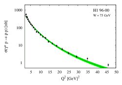
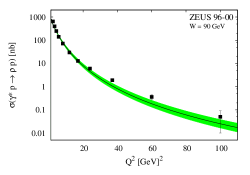
Figure 6: The behaviour according to our model of the $\gamma^{*}p\rightarrow\rho^{0}p$ total cross section as function of $Q^{2}$ is compared with data from Refs. r1 ; r2 measured by the H1 and ZEUS Collaborations for fixed values of $W$. The green bands are calculated accordingly with the uncertainties on the free parameter $|A_{0}|$.

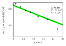
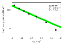
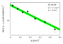
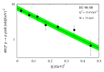
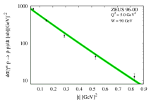
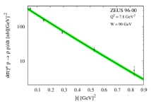
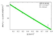
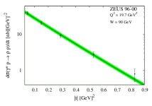
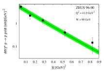
Figure 8: The behaviour of $\gamma^{*}p\rightarrow\rho^{0}p$ differential cross section as function of $t$ is compared with data from Ref. r1 ; r2 measured by the H1 and ZEUS Collaborations for several values of $Q^{2}$ and $W$. The green bands are calculated accordingly with the uncertainties on the free parameter $|A_{0}|$.

All subsequent fits are performed with only $|A_{0}|$ as free parameter. The results for the total cross section as a function of $Q^{2}$ at fixed $W$ and as a function of $W$ at fixed $Q^{2}$, are respectively shown in Figs. 6,  7, and Tables 3, 8. The results for the differential cross section as function of t are shown in Fig. 8, and Table 9.

Table 7: Values of the free parameter $|A_{0}|$ and $\tilde{\chi}^{2}$ from the fit to data from Refs. r1 ; r2 of $\gamma^{*}p\rightarrow\rho^{0}p$ total cross section as function of $Q^{2}$ for fixed values of $W$.

	$\sigma_{(\gamma^{*}~{}p~{}->~{}\rho^{0}~{}p)}(Q^{2})$
Coll.	Years	$W$ [GeV]	$|A_{0}|$ [nb]1/2	$\tilde{\chi}^{2}$
H1	96-00	75	0.885 $\pm$ 0.013	1.4
ZEUS	96-00	90	0.918 $\pm$ 0.021	6.8

Table 8: Values of the free parameter $|A_{0}|$ and $\tilde{\chi}^{2}$ from the fit to data from Ref. r1 of $\gamma^{*}p\rightarrow\rho^{0}p$ integrated cross section as function of $W$ for fixed values of $Q^{2}$.

	$\sigma_{(\gamma^{*}~{}p~{}->~{}\rho^{0}~{}p)}(W)$
Coll.	Years	$Q^{2}$ [GeV2]	$|A_{0}|$ [nb]1/2	$\tilde{\chi}^{2}$
H1	96-00	3.3	0.916 $\pm$ 0.036	3.1
H1	96-00	6.6	0.837 $\pm$ 0.027	2.1
H1	96-00	11.9	0.883 $\pm$ 0.021	0.7
H1	96-00	19.5	0.937 $\pm$ 0.054	4.2
H1	96-00	35.6	1.082 $\pm$ 0.112	3.7
ZEUS	96-00	2.4	1.023 $\pm$ 0.018	1.2
ZEUS	96-00	3.7	0.946 $\pm$ 0.023	4.0
ZEUS	96-00	6.0	0.837 $\pm$ 0.017	2.2
ZEUS	96-00	8.3	0.854 $\pm$ 0.024	4.5
ZEUS	96-00	13.5	0.866 $\pm$ 0.026	5.8
ZEUS	96-00	32.0	1.109 $\pm$ 0.053	3.9

Table 9: Values of the free parameter $|A_{0}|$ and $\tilde{\chi}^{2}$ from the fit to data from Ref. r1 of $\gamma^{*}~{}p\rightarrow\rho^{0}p$ differential cross section as function of t for fixed values of Q² and W.

	$\sigma_{(\gamma^{*}~{}p~{}->~{}\rho^{0}~{}p)}(t)$
Coll.	Years	$W$ [GeV]	$Q^{2}$ [GeV2]	$|A_{0}|$ [nb]1/2	$\tilde{\chi}^{2}$
H1	96-00	75	3.3	0.885 $\pm$ 0.048	5.1
H1	96-00	75	6.6	0.801 $\pm$ 0.039	5.0
H1	96-00	75	11.5	0.872 $\pm$ 0.030	1.1
H1	96-00	75	17.4	0.847 $\pm$ 0.022	0.7
H1	96-00	75	33	0.901 $\pm$ 0.023	0.4
ZEUS	96-00	90	2.7	1.002 $\pm$ 0.038	4.3
ZEUS	96-00	90	5.0	0.867 $\pm$ 0.026	2.8
ZEUS	96-00	90	7.8	0.824 $\pm$ 0.025	2.4
ZEUS	96-00	90	11.9	0.834 $\pm$ 0.019	1.1
ZEUS	96-00	90	19.7	0.946 $\pm$ 0.016	0.4
ZEUS	96-00	90	41.0	1.166 $\pm$ 0.050	0.4

III.2.2 $\gamma^{*}~{}p~{}\rightarrow~{}\phi~{}p$

Experimental data for the fits are taken from Refs. r1 ; phi_zeus . The exploratory fit to determine the weighted average value of $b_{2}$ is shown in Table 10.

Table 10: Values of the two free parameters $|A_{0}|$, $b_{2}$ and $\tilde{\chi}^{2}$, from the two-parameter fit to data from Refs. r1 ; phi_zeus of total cross section of $\gamma^{*}p\rightarrow\phi p$ as function of $Q^{2}$ and fixed values of $W$. The average value of $b_{2}$ was found to be:$<b_{2}>=1.131\pm 0.033$.

	$\sigma_{(\gamma^{*}~{}p~{}->~{}\phi~{}p)}(Q^{2})$
Coll.	Years	$W$ [GeV]	$|A_{0}|$ [nb]1/2	$b_{2}$	$\tilde{\chi}^{2}$
H1	96-00	75	0.390 $\pm$ 0.010	1.155 $\pm$ 0.044	0.9
ZEUS	98-00	75	0.433 $\pm$ 0.011	1.110 $\pm$ 0.050	2.6

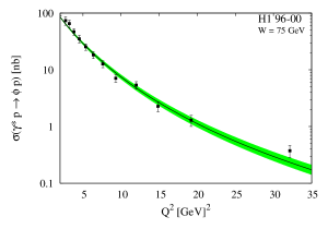
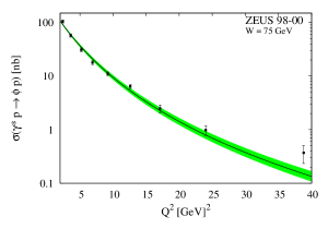
Figure 9: The behaviour of $\gamma^{*}p\rightarrow\phi p$ total cross section as function of $Q^{2}$ is compared to data from Refs. r1 ; phi_zeus measured by the H1 and ZEUS Collaborations for $W=$ 75 GeV. The green bands are calculated accordingly with the uncertainties on the free parameter $|A_{0}|$.

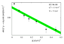
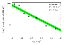
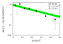
Figure 11: The behaviour according to our model of $\gamma^{*}p\rightarrow\phi p$ differential cross section as function of $t$ is compared with data from Refs. r1 measured by the H1 Collaboration for several values of $Q^{2}$ and $W$. The green bands are calculated accordingly with the uncertainties on the free parameter $|A_{0}|$.

All subsequent fits are performed with only $|A_{0}|$ as free parameter. The results for the total cross section as a function of $Q^{2}$ at fixed $W$ and as a function of $W$ at fixed $Q^{2}$ are respectively shown in Figs. 9, 10, and Tables 11, 15. The results for the differential cross section as function of $t$ are shown in Figs. 11, 12 and Tables 13.

Table 11: Values of the free parameter $|A_{0}|$ and $\tilde{\chi}^{2}$ from the fit to data from Refs. r1 ; phi_zeus of $\gamma^{*}p\rightarrow\phi p$ total cross section as function of $Q^{2}$ and fixed value of $W$.

	$\sigma_{(\gamma^{*}~{}p~{}->~{}\phi~{}p)}(Q^{2})$
Coll.	Years	$W$ [GeV]	$|A_{0}|$ [nb]1/2	$\tilde{\chi}^{2}$
H1	96-00	75	0.387 $\pm$ 0.008	0.8
ZEUS	96-00	75	0.435 $\pm$ 0.010	2.3

Table 12: Values of the free parameter $|A_{0}|$ and $\tilde{\chi}^{2}$ from the fit to data from Ref. r1 of $\gamma^{*}p\rightarrow\phi p$ integrated cross section as function of $W$ for fixed values of $Q^{2}$.

	$\sigma_{(\gamma^{*}~{}p~{}->~{}\phi~{}p)}(W)$
Coll.	Years	$Q^{2}$ [GeV2]	$|A_{0}|$ [nb]1/2	$\tilde{\chi}^{2}$
H1	96-00	3.3	0.397 $\pm$ 0.013	0.9
H1	96-00	6.6	0.362 $\pm$ 0.017	1.7
H1	96-00	15.8	0.423 $\pm$ 0.026	2.1
ZEUS	96-00	2.4	0.462 $\pm$ 0.010	1.1
ZEUS	96-00	3.8	0.431 $\pm$ 0.009	0.8
ZEUS	96-00	6.5	0.401 $\pm$ 0.007	0.4
ZEUS	96-00	13.0	0.470 $\pm$ 0.009	0.4

Table 13: Values of the free parameter $|A_{0}|$ and $\tilde{\chi}^{2}$ from the fit to data from Refs. r1 of $\gamma^{*}~{}p\rightarrow\phi p$ differential cross section as function of t for fixed values of Q² and W.

	$\sigma_{(\gamma^{*}~{}p~{}->~{}\phi~{}p)}(t)$
Coll.	Years	$W$ [GeV]	$Q^{2}$ [GeV2]	$|A_{0}|$ [nb]1/2	$\tilde{\chi}^{2}$
H1	96-00	75	3.3	0.396 $\pm$ 0.026	3.2
H1	96-00	75	6.6	0.358 $\pm$ 0.019	2.1
H1	96-00	75	15.8	0.329 $\pm$ 0.024	2.1
ZEUS	98-00	75	0.0	0.438 $\pm$ 0.015	2.0

III.2.3 $\gamma^{*}~{}p~{}\rightarrow~{}\omega~{}p$

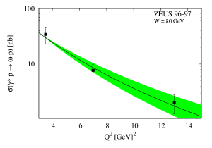
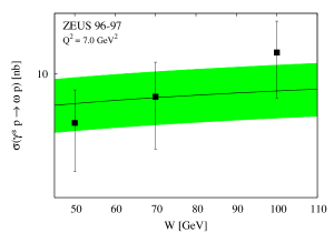
Figure 13: The behaviour according to our model of $\gamma^{*}p\rightarrow\omega p$ total cross section as function of Q² (left) nad $W$ (right) is compared with data from Ref. omega_zeus measured by the ZEUS Collaboration at fixed value of $W$ nas $Q^{2}$ respectively. The green bands are calculated accordingly with the uncertainties on the free parameter $|A_{0}|$.

Experimental data for the fits are taken from Ref. omega_zeus . There only two set of data have been published by the ZEUS Collaboration, one at fixed $W$, the other at fixed $Q^{2}$. No data for the differential cross section as function of $t$ are available. The results for the total cross section as a function of $Q^{2}$ at fixed $W$ and as a function of $W$ at fixed $Q^{2}$ are respectively shown in Fig. 13 and Table 14, 15.

Table 14: Values of the free parameter $|A_{0}|$ and $\tilde{\chi}^{2}$ from the fit to data from Ref. omega_zeus of $\gamma^{*}~{}p\rightarrow\omega p$ total cross section as function of Q² for fixed value of W.

	$\sigma_{(\gamma^{*}~{}p~{}->~{}\omega~{}p)}(Q^{2})$
Coll.	Years	$W$ [GeV]	$|A_{0}|$ [nb]1/2	$\tilde{\chi}^{2}$
ZEUS	96-97	80	0.273 $\pm$ 0.012	0.3

Table 15: Values of the free parameter $|A_{0}|$ and $\tilde{\chi}^{2}$ from the fit to data from Ref. omega_zeus of $\gamma^{*}~{}p\rightarrow\omega p$ total cross section as function of $W$ for fixed value of Q².

	$\sigma_{(\gamma^{*}~{}p~{}->~{}\omega~{}p)}(W)$
Coll.	Years	Q2 [GeV2]	$|A_{0}|$ [nb]1/2	$\tilde{\chi}^{2}$
ZEUS	96-97	7.0	0.265 $\pm$ 0.022	0.5

III.2.4 $\gamma^{*}~{}p~{}\rightarrow~{}J/\psi~{}p$

Experimental data for the fits are taken from Refs. j1 ; j2 . The exploratory fit to determine the weighted average value of $b_{2}$ gives a result which is shown in Table 16.

Table 16: Values of the two free parameters $|A_{0}|$, $b_{2}$ and $\tilde{\chi}^{2}$, from the two-parameter fit to data from Refs. j1 ; j2 of the total cross section of $\gamma^{*}p\rightarrow J/\psi p$ as function of $Q^{2}$ and fixed $W$. The average value of $b_{2}$ was found to be: $<b_{2}>=0.890\pm 0.033$.

	$\sigma_{(\gamma^{*}~{}p~{}->~{}J/\psi~{}p)}(Q^{2})$
Coll.	Years	$W$ [GeV]	$|A_{0}|$ [nb]1/2	$b_{2}$	$\tilde{\chi}^{2}$
H1	99-00	90	0.855 $\pm$ 0.031	0.898 $\pm$ 0.033	0.4
ZEUS	98-00	90	0.853 $\pm$ 0.040	0.879 $\pm$ 0.035	0.7

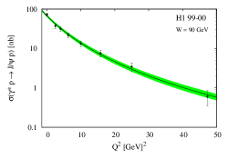
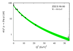
Figure 14: The behaviour according to our model of $\gamma^{*}p\rightarrow J/\psi p$ total cross section as function of $Q^{2}$ is compared with data from Refs. j1 ; j2 measured by the H1 and ZEUS Collaborations for $W=90$ GeV. The green bands are calculated accordingly with the uncertainties on the free parameter $|A_{0}|$.

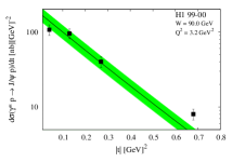
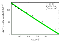
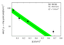
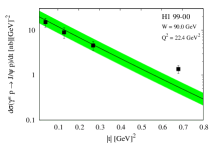
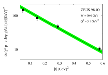
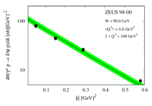
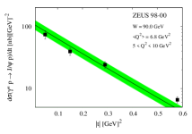
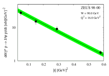
Figure 16: The behaviour according to our model of $\gamma^{*}p\rightarrow J/\psi p$ differential cross section as function of $t$ is compared with data from Ref. j1 ; j2 measured by the H1 and ZEUS Collaborations for several values of $Q^{2}$ and fixed $W$. The green bands are calculated accordingly with the uncertainties on the free parameter $|A_{0}|$.

All subsequent fits are performed with only $|A_{0}|$ as free parameter. The result for the total cross section as a function of $Q^{2}$ at fixed $W$ and as a function of $W$ at fixed $Q^{2}$ are respectively shown in Figs. 14, 15, and Tables 16, 18. The results for the differential cross section as function of $t$ are shown in Fig. 16 and Table 19.

Table 17: Values of the free parameter $|A_{0}|$ and $\tilde{\chi}^{2}$ from the fit to data from Refs. j1 ; j2 of the $\gamma^{*}p\rightarrow J/\psi p$ total cross section as function of $Q^{2}$ for fixed value of $W$.

	$\sigma_{(\gamma^{*}~{}p~{}->~{}J/\psi~{}p)}(Q^{2})$
Coll.	Years	$W$ [GeV]	$|A_{0}|$ [nb]1/2	$\tilde{\chi}^{2}$
H1	99-00	90	0.857 $\pm$ 0.013	0.4
ZEUS	98-00	90	0.875 $\pm$ 0.014	0.6

Table 18: Values of the free parameter $|A_{0}|$ and $\tilde{\chi}^{2}$ from the fit to data from Refs. j2 of $\gamma^{*}~{}p\rightarrow J/\psi p$ total cross section as function of $W$ for fixed values of Q².

	$\sigma_{(\gamma^{*}~{}p~{}->~{}J/\psi~{}p)}(W)$
Coll.	Years	Q2 [GeV2]	$|A_{0}|$ [nb]1/2	$\tilde{\chi}^{2}$
H1	99-00	3.2	0.790 $\pm$ 0.037	1.3
H1	99-00	7.0	0.768 $\pm$ 0.050	1.4
H1	99-00	22.4	0.916 $\pm$ 0.044	0.7
ZEUS	98-00	0.4	0.867 $\pm$ 0.111	4.0
ZEUS	98-00	3.1	0.840 $\pm$ 0.043	2.1
ZEUS	98-00	6.8	0.844 $\pm$ 0.033	1.4
ZEUS	98-00	16.0	0.815 $\pm$ 0.078	5.8

Table 19: Values of the free parameter $|A_{0}|$ and $\tilde{\chi}^{2}$ from the fit to data from Ref. j2 of $\gamma^{*}~{}p\rightarrow J/\psi p$ differential cross section as function of $t$ for fixed values of Q² and W.

	$\sigma_{(\gamma^{*}~{}p~{}->~{}J/\psi~{}p)}(t)$
Coll.	Years	$W$ [GeV]	$Q^{2}$ [GeV2]	$|A_{0}|$ [nb]1/2	$\tilde{\chi}^{2}$
H1	99-00	90	0.05	0.860 $\pm$ 0.035	5.1
H1	99-00	90	3.2	0.778 $\pm$ 0.066	4.1
H1	99-00	90	7.0	0.710 $\pm$ 0.083	4.3
H1	99-00	90	22.4	0.861 $\pm$ 0.090	3.0
ZEUS	98-00	90	3.1	0.868 $\pm$ 0.031	0.9
ZEUS	98-00	90	6.8	0.841 $\pm$ 0.033	2.9
ZEUS	98-00	90	6.8	0.824 $\pm$ 0.049	3.3
ZEUS	98-00	90	16.0	0.863 $\pm$ 0.023	0.5

IV Conclusions and Outlooks

In this paper we have revised and extended the model of Ref. DVCS to include, apart from DVCS, vector meson production as well. The basic features of the model here remain intact, but the fitting procedure has changed. On one hand, the parameters entering the Pomeron trajectory and the coefficient $b_{1}$ in the residue of the proton ($pI\!\!Pp$) vertex are the same for DVCS and VMP processes. In particular, the parameter $b_{1}$ is known, due to Regge factorization, from $pp$ and $\bar{p}$p scattering and set to the value $b_{1}=2.0$, related to the proton radius. On the other hand, the normalization parameter $A_{0}$ and the coefficient $b_{2}$ in the residue of the photon $\gamma^{*}I\!\!P\gamma$ vertex are different for each reaction we considered in this paper (production of a real $\gamma$ or $\rho$, $\ \ \phi$,   $\omega$ and $J/\Psi$ vector mesons). In particular, for each reaction the parameter $b_{2}$ first has been fitted to the existing sets of experimental data on the total cross section as a function of the virtuality $Q^{2}$, then it has been fixed to the average value among those obtained from the fits. Consequently, fits to experimental data on differential cross section and total cross section as a function of the energy $W$ have been performed, the normalization $A_{0}$ being the only free parameter. All experimental data used in the fitting procedure were selected by the H1 and ZEUS collaborations as diffractive ones, therefore there is no place for any secondary (nonleading) Regge contribution, the Pomeron trajectory being the only $t$ channel contribution, and hence the often used notion of an effective trajectory, in this paper means the genuine Pomeron.

It is always instructive to compare the Pomeron trajectory deduced from DVCS and VMP production data with that extracted from hadronic scattering. Since the Pomeron trajectory is universal and the precision of the high-energy $pp$ and $\bar{p}p$ data exceeds those of DVCS or VMP, it makes sense to use for it values of parameters resulting from fits to the former data.

Here we come to the important question of how many Pomerons exist in nature. Our answer is that there is only one Pomeron and it is universal, which does not mean that it is simple. Moreover, it may have more components, whose relative weight is governed by their residue.

By assuming the universality of the Pomeron trajectory in lepton-hadron and hadron-hadron reactions, one expects that the effect of its non-linearity be visible also in $pp$ scattering, say in the ISR energy region comparable to typical HERA energies. Indeed, as shown in a series of papers Enrico , the flattening of the differential cross section of $pp$ scattering beyond the dip, fitted by Donnachie and Landshoff by a power $t^{-n}$ can equally well be attributed by the logarithmic behavior of the Pomeron trajectory, mimicking this hard power behavior.

In the present paper we adopted the simple case of a soft Pomeron. The presence of another hard component here was not considered. The delicate interplay of soft and hard components (in a single Pomeron) is governed by the external masses and virtualities in the residues as shown in Ref DL . We intend to come back to this point in a forthcoming study. As expected, our model leads to results on the whole satisfactory for moderate values of $\tilde{Q}^{2}$ and $|t|$. Instead, without a hard component in the Pomeron, fits to the data for high $\tilde{Q}^{2}$ and $|t|$ definitely deteriorate.

Finally, let us come back to one of the main ingredients of the model we considered in the present paper, namely to the variable $z=t-Q^{2}$. This is an unusual combination of the squared momentum transfer $t$ and virtuality $Q^{2}$ ; it does not follow from the theory, although it appears also e.g. in the expression for the slope $B(Q^{2},t)$ in Refs. R1 ; R2 . These two variables not only have similar dimensions, but have also close physical meanings, so we could say that high values of the variable $z$ are correlated with a hard component in the Pomeron.

In fact, as seen from Fig. 2, our non-linear Pomeron trajectory, in the region $-1.0<t<0$ GeV² does not differ significantly from the linear one e.g. in Refs. L . The use of the non-linear trajectories is motivated: 1) conceptually, by the expected large-$|t|$ scaling behavior (not reached yet experimentally) and 2) by the large-$Q^{2}$ data, already experimentally accessible.

In the spirit of the Regge-pole theory, we have taken into account Regge-factorization of the lower vertex and the propagator by keeping them $t-$dependent only, while the upper $\gamma^{*}I\!\!P\gamma$ vertex depends also on $Q^{2}.$ At the same time, considering the Regge-exchange as an effective one, one must not respect this factorization since the corresponding effective amplitude absorbs various Regge-exchanges anyway.

Since the H1 and ZEUS data, both on DVCS and VMP are well within the Regge kinematical region, we used the Regge-factorized form, according to which the scattering amplitude corresponding to the exchange of a single Regge-trajectory is the product of the two vertices and the Pomeron propagator. Actually, the sum of different Regge-pole exchanges often is comprised in a single effective pole, which however should not be confused with a true Regge-pole.

Most of our figures presenting the $W$ dependence of the various channels underestimate the high-energy tail of the data. In our opinion, this is a strong evidence in favor of a Pomeron having two components, hard and soft, their relative weights depending on $\tilde{Q}^{2}$, as advocated in Ref. DL . The presence of a hard component, with a Pomeron intercept as high as $1.3-1.4$ will require unitarization. In a forthcoming study, based on Reggeometry FFJL , we plan to extend the model to high values of $Q^{2}$ and $|t|$ by introducing a hard component in the single universal Pomeron.

Our final comment is that our model should be used as a guide in building explicit expressions for General Parton Distributions.

*

Appendix A

Here we present the calculation of the integrated cross section with the non linear trajectory given in Eqs. (2) and (4) and entering the amplitude (5). The cross section is defined as

$$\sigma(s,\tilde{Q}^{2})=\int^{-4m^{2}_{p}}_{-s/2}~{}dt~{}{\frac{d\sigma(s,t,\tilde{Q}^{2})}{dt}}.$$ (12)

In the limit of very high energy ($s\rightarrow\infty$) and negligible proton mass it becomes

$$\sigma(s,\tilde{Q}^{2})=\int^{\infty}_{0}~{}dt~{}\frac{d\sigma(s,t,\tilde{Q}^{2})}{dt},$$ (13)

where the change $t\rightarrow-t$ has been applied.

Substituting the expression (6) for the differential cross section, using Eq. (5) for the amplitude and with the replacement $x=\alpha_{2}t$, this cross section assumes the form GrRy

$$\sigma(s,\tilde{Q}^{2}) = \int^{\infty}_{0}dx~{}(1+x)^{-\mu+\nu}(\beta+x)^{-\nu}$$ (14)

$$= KB(\mu-1,1)_{~{}2}F_{1}\left(\nu,\mu-1;\mu;1-\beta\right)~{}~{}~{}~{}~{}~{}~{}~{}$$

with

$$K = \frac{\pi|A_{0}|^{2}}{\alpha_{2}~{}s^{2}}e^{2\alpha_{0}(b_{1}+b_{2})}(s/s_{0})^{2\alpha_{0}},$$

$$\beta = 1+\alpha_{2}\tilde{Q}^{2},$$

$$\nu = 2b_{2}\alpha_{1},$$

$$\mu = 2\alpha_{1}\left[b_{1}+b_{2}+\ln(s/s_{0})\right]>1.$$

Here $B(\mu-1,1)=1/(\mu-1)$ is our $Beta$ function and ${}_{~{}2}F_{1}\left(\nu,\mu-1;\mu;1-\beta\right)$ is the Gauss hypergeometric function. Then our final expression for the integrated cross section is

$$\sigma(s,\tilde{Q}^{2})=\frac{K}{\mu-1}{~{}_{2}}F_{1}\left(\nu,\mu-1;\mu;1-\beta\right).$$ (15)

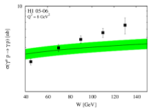
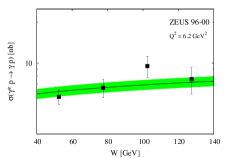
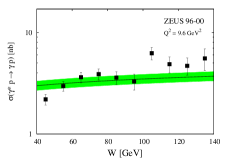
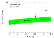
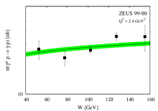
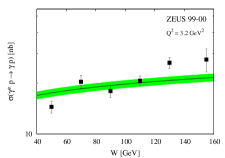
Figure 4: The behaviour according to our model of $\gamma^{*}p\rightarrow\gamma p$ total cross section as function of $W$ is compared with data from Refs. d1 ; d3 ; d4 measured by the H1 and ZEUS Collaborations for several values of $Q^{2}$. The green bands are calculated according with the uncertainties on the free parameter $|A_{0}|$.

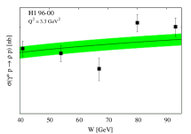
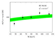
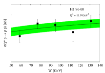
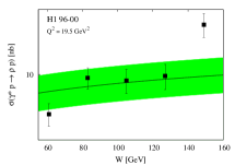
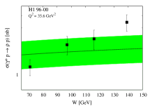
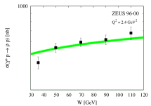
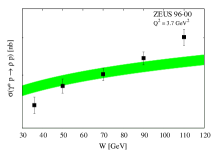
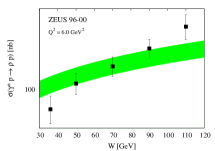
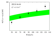
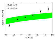
Figure 7: The behaviour according to our model of the $\gamma^{*}p\rightarrow\rho^{0}p$ total cross section as function of $W$ is compared with data from Ref. r1 ; r2 measured by the H1 and ZEUS Collaborations for several values of $Q^{2}$. The green bands are calculated according with the uncertainties on the free parameter $|A_{0}|$.

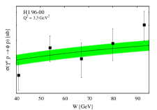
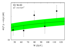
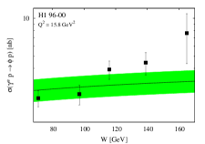
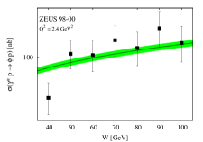
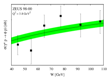
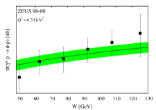
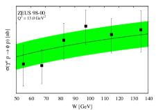
Figure 10: The behaviour of $\gamma^{*}p\rightarrow\phi p$ total cross section as function of $W$ is compared to data from Ref. r1 ; phi_zeus measured by the H1 and ZEUS Collaborations for several values of $Q^{2}$. The green bands are calculated according with the uncertainties on the free parameter $|A_{0}|$.

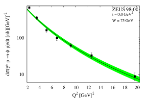
Figure 12: The behaviour according to our model of $\gamma^{*}p\rightarrow\phi p$ differential cross section as function of Q² is compared with data from Refs. phi_zeus measured by the ZEUS Collaboration for fixed values $W$ and $t$. The green bands are calculated accordingly with the uncertainties on the free parameter $|A_{0}|$.

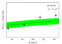
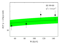
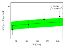
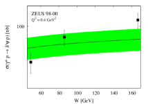
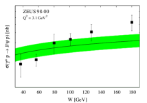
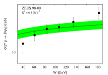
Figure 15: The behaviour according to our model of $\gamma^{*}p\rightarrow J/\psi p$ total cross section as function of $W$ is compared with data from Ref. j1 ; j2 measured by the H1 and ZEUS Collaborations for several values of $Q^{2}$. The green bands are calculated accordingly with the uncertainties on the free parameter $|A_{0}|$.

References

- (1) M. Capua, S. Fazio, R. Fiore, L.L. Jenkovszky, and F. Paccanoni, Phys. Lett. B645 (2007) 161.
-
(2)
I.P. Ivanov, N.N. Nikolaev, and A.A. Savin, Phys. Part. Nucl. 37 (2006) 1, DESY 04-243 preprint, [hep-ph/0501034];
-
(3)
H. Fraas and D. Schildknecht, Nucl. Phys. B14 (1969) 543;
D. Schildknecht, G.A. Schuler, and B. Surrow, Phys. Lett. B449 (1999) 328, CERN-TH-98-294, [hep-ph/9810370]. - (4) P. Landshoff, Fundamental problems with hadronic and leptonic interactions, [hep-ph/0903.1523].
- (5) A. Donnachie and P.V. Landshoff, Successful description of exclusive vector meson electroproduction, DAMTP-2008-3, MAN-HEP-2008-1, [hep-ph/0803.0686].
-
(6)
L.L. Jenkovszky, Rivista Nuovo Cim., 10 (1987) 1;
M. Bertini et al. ibid 19 (1996) 1. - (7) R. Fiore, L.L. Jenkovszky, V.K. Magas, and F. Paccanoni, Phys. Rev. D60 (1999) 116003, [hep-ph/9904202].
-
(8)
E.A Kuraev,L.N. Lipatov, and V.S .Fadin, Zh.Eksp.Teor.Fiz. 72 (1977) 377 [Sov. Phys. JETP 45 (1977) 199];
Ya.Ya. Balitsky and L.N. Lipatov, Sov. J.Nucl.Phys. 28 (1978) 822;
L.N. Lipatov, Zh. Eksp. Teor. Fiz. 90 (1986) 1536 [Sov. Phys. JEPT B63 (1986) 904]. - (9) D. Boer et al., Gluons an the quark sea at high energies: distributions, polarization, tomography, arXiv:1108.1713 [nucl-th].
-
(10)
V.N. Gribov and L.N. Lipatov. Sov.J.Nucl.Phys. 15 (1972) 438;
G. Altarelli and G. Parisi, Nucl. Phys. B 126 (1977) 298;
Yu. L. Dokshitzer. Sov.Phys, JETP 46 (1977) 641. - (11) L. Csernai, L.L. Jenkovszky, K. Kontros, A. Lengyel, V.K. Magas, and F. Paccanoni, Eur. Phys. J. C24 (2002) 205, [hep-ph/0112265].
-
(12)
S.M. Troshin, N.E. Tyurin, Eur. Phys. J. C. 22 (2002) 667;
M.A. Perfilov, S.M. Troshin, Mass dependence in vector meson electroproduction, [hep-ph/0207306];
S.M. Troshin, N.E. Tyurin, Regularities of vector meson electroproduction: Transitory effects or early asymptotics?, [hep-ph/0301112]. - (13) D. Mueller, Pomeron dominance in deeply virtual Compton scattering and the femto holographic image of the proton, [hep-ph/0605013].
- (14) S. Fazio, R. Fiore, L.L. Jenkovszky, A. Lavorini, and A. Salij, Reggeometry in DVCS and VMP, in preparation.
- (15) V. Barone and E. Predazzi, High-energy Particle Diffraction, Springer-Verlag, 2002.
- (16) R. Fiore, L.L. Jenkovszky, and F. Paccanoni, Eur. Phys. J., CIO (1999), [hep-ph/9812458]
- (17) H1 Coll., A. Atkas et al., Eur. Phys. J. C44 (2005) 1, DESY-05-065 preprint, [hep-ex/0505061].
- (18) H1 Coll., F. D. Aaron et al., Phys. Lett. B659 (2008) 796, DESY-07142 preprint, arXiv:0709.4114 [hep-ex].
- (19) H1 Coll., F. D. Aaron et al., Phys. Lett. B681 (2009) 391, DESY 09-109 preprint, arXiv:0907.5289 [hep-ex].
- (20) ZEUS Coll., S. Chekanov et al., JHEP 0905 (2009) 108, DESY 08-132 preprint, arXiv:0812.2517 [hep-ex].
- (21) H1 Coll., F. D. Aaron et al., JHEP 1005 (2010) 032, DESY 09-093 preprint, arXiv:0910.5831 [hep-ex].
- (22) ZEUS Coll., S. Chekanov et al., PMC Phys. A1 (2007) 6, DESY 07-118 preprint, arXiv:0708.1478 [hep-ex].
- (23) ZEUS Coll., S. Chekanov et al., DESY-05-038 preprint, Nucl. Phys. B718 (2005) 3, DESY-05-038 preprint, [hep-ex/0504010].
- (24) ZEUS Coll., J. Breitweg et al., Phys. Lett. B487 (2000) 3-4, 273, DESY-00-084 preprint, [hep-ex/0006013].
- (25) ZEUS Coll., S. Chekanov et al., Nucl. Phys. B695 (2004) 3, DESY 04-052 preprint, [hep-ex/0404008].
- (26) H1 Coll., A. Atkas et al., Eur. Phys. J. C46 (2006) 585, DESY 05-161 preprint, [hep-ex/0510016].
- (27) A.D. Martin, M.G. Ryskin and T. Teubner, Phys. Rev. D 62 (2000) 014022, hep-ph/9912551.
- (28) M.G. Ryskin, Yu.M. Shabelski, A.G. Shuvalov, Phys. Lett. B 446 (1998) 395, hep-ph/9802366.
- (29) Gradshteyn and Ryzhik, Table of Integrals, Series, and Products, Academic Press, 2007.
-
(30)
R.J.M. Covolan, L.L. Jenkovszky, E. Predazzi, Z. Phys. C 51 (1991) 456;
P. Desgrolard, M. Giffon, L.L. Jenkovszky, Z. Phys. 55 (1992) 637;
R.J.M. Covolan et al., Z.Phys. C. 58 (1993) 109.