Testing nonstandard cosmological models with SNLS3 supernova data and other cosmological probes

Abstract

We investigate the implications for some nonstandard cosmological models using data from the first three years of the Supernova Legacy Survey (SNLS3), assuming a spatially flat universe. A comparison between the constraints from the SNLS3 and those from other SN Ia samples, such as the ESSENCE, Union2, SDSS-II and Constitution samples, is given and the effects of different light-curve fitters are considered. We find that SN Ia with SALT2 or SALT or SIFTO can give consistent results and the tensions between different data sets and different light-curve fitters are obvious for fewer-free-parameters models. At the same time, we also study the constraints from the SNLS3 along with data from the cosmic microwave background and the baryonic acoustic oscillations (CMB/BAO), and the latest Hubble parameter versus redshift (H(z)). Using model selection criteria such as $\chi^{2}$/dof, GoF, AIC and BIC, we find that, among all the cosmological models considered here ($\Lambda$CDM, constant $w$, varying $w$, DGP, modified polytropic Cardassian, and the generalized Chaplygin gas), the flat DGP is favored by the SNLS3 alone. However, when additional CMB/BAO or H(z) constraints are included, this is no longer the case, and the flat $\Lambda$CDM becomes preferred.

1 INTRODUCTION

Type Ia supernovae (SNe Ia) have altered the focus of cosmology dramatically since they first indicated that the expansion of the Universe is currently accelerating (Riess et al., 1998; Perlmutter et al., 1999). Usually, the mysterious cause of the cosmic acceleration is attributed either to the existence of an exotic energy component, called dark energy, or a modification of the standard theory of gravity. At present, SNe Ia are still the most direct probe of the history of cosmic expansion and the properties of dark energy, and many SN Ia samples, such as ESSENCE (Wood-Vasey et al., 2007), SDSS-II (Kessler et al., 2009), Constitution (Hicken et al., 2009) and Union2 (Amanullah et al., 2010), have been released.

The Supernova Legacy Survey (SNLS) is an ongoing five year project that aims to probe the expansion history of the universe using SNe Ia (Sullivan et al., 2005). The goal of this survey is to measure the time-averaged equation of state (EOS) of dark energy ($w$) to $5\%$ (statistical uncertainties only) in combination with other cosmological probes and to $10\%$ including the systematic uncertainties. Analysis of the first year of data from SNLS, containing 71 high-redshift SNe Ia, was presented in Astier et al. (2006).

Recently, data from the first three years SNLS data set were released. Guy et al. (2010, hereafter G10) presented the photometric properties and relative distance moduli of 252 SNe Ia from this sample. Based on selection criteria, they removed 21 SNe and obtained $\Omega_{m}=0.211\pm 0.034(\mathrm{stat})\pm 0.069(\mathrm{sys})$ for a flat $\Lambda$CDM using the SNLS3 data alone. Using a slightly different set of selection criteria, Conley et al. (2011, hereafter C11) selected 242 SNe Ia from SNLS, and combined these with 123 low-$z$, 93 intermediate-$z$ (SDSS-II) and 14 high-$z$ SNe from the Hubble Space Telescope to form a high-quality unified sample containing 472 SNe Ia. We shall refer to this sample as SNLS3. For the SNLS3 data alone, C11 finds that $w=-0.91^{+0.16}_{-0.20}(\mathrm{stat})^{+0.07}_{-0.14}(\mathrm{sys})$, considering a flat Universe with constant $w$. The constraints on dark energy when SNLS3 is combined with other probes (such as the baryonic acoustic oscillation (BAO) (Percival et al., 2009) or WMAP7 (Komatsu et al., 2011)) were presented in Sullivan et al. (2011, hereafter S11). The results for a flat constant $w$ universe are $\Omega_{m}=0.269\pm 0.015$ and $w=-1.061^{+0.069}_{-0.068}$, and those for a flat varying $w$ universe characterized by the CPL parameterization (Chevallier & Polarski, 2001; Linder, 2003) ($w(a)=w_{0}+w_{a}(1-a)$) are $w_{0}=-0.905\pm 0.196$ and $w_{a}=-0.984^{+1.094}_{-1.097}$.

Dark energy is not the only possible explanation of the present cosmic acceleration, and many other models have been considered such as DGP, Cardassian, and the generalized Chaplygin gas. In this paper we investigate constraints on these nonstandard cosmological models. Similar analyses were carried out by Davis et al. (2007) and  Sollerman et al. (2009) using the ESSENCE (Wood-Vasey et al., 2007) and SDSS-II (Kessler et al., 2009) SN Ia data sets, respectively. In order to give a comparison between the results from SNLS3 with those from other SN Ia data sets, we also compare the constraints obtained using SNLS3 to those using other popular SNe Ia samples such as the ESSENCE, Constitution, Union2 and SDSS-II samples, and additionally analyze the effects of different light-curve fitters on the results. In addition to the SNe Ia data, constraints from other probes, such as the cosmic microwave background (CMB) and baryonic acoustic oscillations (BAO) measurements of the acoustic scale (CMB/BAO) and the Hubble parameter vs. redshift (H(z)), are also considered.

We organize our paper as follows. Section 2 presents the data sets and the statistical analysis method. Section 3 describes briefly the models considered and the observational constraints on them. Model testing results using model selection statistics are shown in section 4. Finally, Section 5 gives a summary of our results.

2 DATA SETS AND ANALYSIS METHODS

In this Section, we describe the data sets and analysis techniques.

2.1 Type Ia supernovae

The SNLS3 SN Ia sample has been discussed in detail in C11. This sample consists of 472 SNe Ia (123 low-$z$, 93 SDSS, 242 SNLS, and 14 $Hubble~{}Space~{}Telescope$) and is compiled with the combined SiFTO (Conley et al., 2008) and SALT2 (Guy et al., 2007) light curve fitters. As discussed in S11, the SNLS3 data set has several advantages over the first year sample presented in Astier et al. (2006). First of all, the sample size has increased by a factor of three. Furthermore, the sources of potential astrophysical systematics are examined by dividing the SN Ia sample according to the properties of either the SN or its environment (Sullivan et al., 2010). Finally, an ameliorated photometric calibration of the light curves and a more consistent understanding of the experimental characteristics are allowed (Regnault et al., 2009).

For the cosmological analysis, one can minimize the following $\chi^{2}$,

$$\chi^{2}=\sum_{\mathrm{SN}}\frac{(m_{B}-m_{B}^{mod})^{2}}{\sigma^{2}_{stat}+\sigma^{2}_{int}},$$ (1)

where $m_{B}$ is the rest-frame $B$-band magnitude of an SN, $m_{B}^{mod}$ is the magnitude of the SN predicted by the cosmological model, $\sigma_{stat}$ includes the uncertainties both in $m_{B}$ and $m_{B}^{mod}$ and $\sigma_{int}$ parameterizes the intrinsic dispersion of each SN sample. The values for $\sigma_{int}$ used in our analysis can be found in Table 4 in C11. The model-dependent magnitude is given by

$$m_{B}^{\mathrm{mod}}=5\log_{10}\mathcal{D}_{L}(z_{\mathrm{hel}},z_{\mathrm{cmb}};\mathbf{p})-\alpha(s-1)+\beta\mathcal{C}+\mathcal{M}_{B},$$ (2)

where $\mathbf{p}$ stands for the model parameters set, $\mathcal{D}_{L}$ is the Hubble-constant free luminosity distance, $z_{\mathrm{hel}}$ and $z_{\mathrm{cmb}}$ are the heliocentric and CMB frame redshifts of the SN, and $\alpha$ and $\beta$ characterize the stretch and color ($s$ and $\mathcal{C}$)-luminosity relationships. $\mathcal{M}_{B}$ represents some combination of the absolute magnitude of a fiducial SN Ia and the Hubble constant. Here, $\alpha$, $\beta$ and $\mathcal{M}_{B}$ are “nuisance parameters”. We marginalize over $\mathcal{M}_{B}$ by following the method described in C11 (Appendix C). In this marginalization method the environmental dependence of SN properties, which allows $\mathcal{M}_{B}$ to be split by host-galaxy stellar mass at $10^{10}M_{\odot}$ (this correction is not employed for all other SN Ia samples we are considering), is taken into account. Defining the vector of residuals between the model magnitudes and the observed magnitudes $\Delta\mathbf{\vec{m}}=\mathbf{\vec{m}}_{B}-\mathbf{\vec{m}}_{B}^{\mathrm{mod}}$, we obtain the observational constraints on model parameters by minimizing

$$\chi^{2}_{SN}=\Delta\mathbf{\vec{m}}^{T}\cdot\mathbf{C}^{-1}\cdot\Delta\mathbf{\vec{m}},$$ (3)

where $\mathbf{C}^{-1}$ is the inverse covariance matrix . The total covariance matrix is detailed in section 3.1 in C11. The covariances which take both statistical and systematic uncertainties into consideration are used in our investigation. We allow $\alpha$ and $\beta$ to vary with the cosmological parameters to avoid biasing our results using a grid $\chi^{2}$ minimization routine and then use their best fit results to obtain the allowed regions of model parameters.

It is well-known that to obtain the precise distance of the standard candle, SNe Ia, is crucial for modern cosmology. Since the intrinsic luminosity of SNe Ia is correlated with the shape of its optical light curves, one can determine it by proposing a method to relate them. Phillips (1993) firstly introduced a method by finding a correction between the SNe Ia intrinsic luminosity and the parameter $\Delta m_{15}(B)$, where $\Delta m_{15}(B)$ is the amount of a SNe Ia B-band declination during the first fifteen days after maximum light. The MLCS is a different method using the multicolor light curve shapes to estimate the luminosity distance proposed in Riess et al. (1995). This approach was extended to include U-band measurements, named MLCS2k2, by Jha (2002). The MLCS2k2 has been applied for distance estimate in several popular SN Ia samples, such as ESSENCE, SDSS-II, and Constitution.

Guy et al. (2005) proposed another method, SALT, to construct the SNe Ia luminosity distance estimate by parameterizing the light curve with a parameter set, i.e., a luminosity parameter, a decline rate parameter and a single color parameter. It offers a practical advantage which makes it easily applicable to high-redshift SNe Ia. By including spectroscopic data, Guy et al. (2007) improved this SALT to SALT2. SALT2 has been applied to calculate the distance modulus for several popular SN Ia samples, such as Constitution, Union2, SDSS-II, and SNLS3. It is notable that the SDSS-II corrected the SALT2 results for selection biases by using a Monte Carlo simulation (see section 5.2 and section 6 of Kessler et al. 2009) and the SNLS team made a few technical modifications in the training procedure, such as higher resolution for the components and the color variation law, and a new regularisation scheme, to SALT2 for the SNLS3 (detailed in section 4.3 and Appendix A of Guy et al. 2010). Recently, Conley et al. (2008) proposed another new empirical way, i.e., SiFTO, which is similar to SALT2 using the luminosity magnitude, light curve shape and color to obtain the distance. This method has been applied in the analysis of SNLS3.

Previous works have shown that different SN Ia data sets give different results (Rydbeck et al., 2007; Bueno Sancheza et al., 2009) and different light-curve fitters may also lead to different conclusions although the same SN Ia sample is considered (Sollerman et al., 2009; Bengochea, 2011). Therefore, in the present paper, besides the SNLS3 (analyzed with SALT2 and SiFTO light-curve fitters), we also consider some other popular SN compilations: ESSENCE (SALT and MLCS2k2), Constitution (SALT2 and MLCS2k2 with $R_{V}=1.7$), Union2 (SALT2) and SDSS-II (SALT2 and MLCS2k2). However, it should be mentioned that these SN Ia samples are not independent, since many of them are drawn from the same sources. That is , different SN Ia compilations may contain many of the same SNe. For instance, the nearby (Jha et al., 2007) and SNLS (Astier et al., 2006) SN Ia are, in part, included as subsets in all above mentioned samples. In addition, except for the Union2 and SNLS3, there is no easy way to include systematic uncertainties for other referred SN samples. In our analysis only for the SNLS3 sample are the systematic uncertainties considered.

2.2 The Cosmic Microwave Background and Baryon Acoustic Oscillations

The CMB and BAO constraints used in this analysis are based on the angular scales measured at the CMB decoupling epoch at $z_{*}=1090$ and imprinted in the clustering of luminous red galaxies (BAO) at $z=[0.2,0.35]$. Its acoustic scale is given by

$$l_{A}=\pi\frac{d_{A}(z_{*})(1+z_{*})}{r_{s}(z_{*})},$$ (4)

which represents the angular scale of sound horizon at decoupling, where $d_{A}=d_{L}/(1+z)^{2}$ is the proper (not comoving) angular diameter distance, $d_{L}=(1+z)\int_{0}^{z}\frac{dz}{H}$ is the luminosity distance, and $r_{s}(z_{*})$ is the comoving sound horizon at recombination,

$$r_{s}(z_{*})=\int_{z_{*}}^{\infty}\frac{c_{s}(z)}{H(z)}dz$$ (5)

which depends on the speed of sound, $c_{s}$, in the early universe. The BAO scale is given by $r_{s}(z_{d})/D_{V}$, where the $r_{s}(z_{d})$ is the comoving sound horizon at drag epoch ($z_{d}\approx 1020$), and the so-called dilation scale, $D_{V}$, is a combination from angular diameter distance and radial distance according to

$$D_{V}(z)=\bigg{[}(1+z)^{2}d_{A}^{2}\frac{cz}{H(z)}\bigg{]}^{1/3}.$$ (6)

By combining the BAO measurements of $r_{s}(z_{d})/D_{V}(z)$ at two redshifts (Percival et al., 2007), $r_{s}(z_{d})/D_{V}(0.2)=0.1980\pm 0.0058$ and $r_{s}(z_{d})/D_{V}(0.35)=0.1094\pm 0.0033$, with the CMB measurement of $l_{A}$ given in Komatsu et al. (2009), $l_{A}=302.10\pm 0.86$, and considering the ratio of the sound horizon at the two epochs, $r_{s}(z_{d})/r_{s}(z_{*})=1.044\pm 0.019$, the final constraints we use for the cosmology analysis are obtained:

$$f_{0.20}=\frac{d_{A}(z_{*})(1+z_{*})}{D_{V}(z=0.2)}=19.04\pm 0.58$$ (7)

$$f_{0.35}=\frac{d_{A}(z_{*})(1+z_{*})}{D_{V}(z=0.35)}=10.52\pm 0.32,$$ (8)

which do not depend on the comoving sound horizon scale at recombination. However, these two ratios are not independent with a correlation coefficient of $0.39$. This correlation is considered in our cosmological fits. Moreover, the constraints from these two ratios (labeled CMB/BAO here) are expected to be a good approximation for all models tested in this paper since the redshift difference between the decoupling and the drag epoch is relatively small, and the sound horizon at these two epoch is mostly dominated by the fractional difference between the number of photons and baryons (Sollerman et al., 2009).

In addition, we do not use the CMB “shift parameters” ($l_{A},R,z_{*}$) derived from WMAP7 (Komatsu et al., 2011) in our analysis, because the CMB distance prior is applicable only when the model in question is based on the standard Friedmann-Lemaitre-Robertson-Walker universe with matter, radiation, dark energy and spatial curvature (Komatsu et al., 2011), and we are testing some nonstandard models, e.g. DGP and modified polytropic Cardassian.

2.3 Hubble parameter versus redshift data

The Hubble parameter versus redshift data to be used in this paper consists of three subsamples. The first one includes 9 data points which are derived from differential ages of old passively evolving galaxies (Simon et al., 2005). The second two-points subsample is determined from the high-quality spectra with the Keck-LRIS spectrograph of red-envelope galaxies in the redshift range $0.2<z<1$ (Stern et al., 2010). The third subsample contains three data points obtained by using the 2-point correlation of SDSS luminous red galaxies and taking the BAO peak position as a standard ruler in the radial direction (Gaztanaga et al., 2009). These three points are considered as a direct measurement of H(z) for the first time and are independent of the earlier BAO measurements (Percival et al., 2007) which constrains an integral of H(z) by using the spherically averaged (monopole) correlation. The parameters set can be determined by minimizing

$${}\chi^{2}_{\mathrm{H(z)}}=\sum_{i=1}^{14}\frac{[H_{th}(z_{i};\mathbf{p})-H_{obs}(z_{i})]^{2}}{\sigma^{2}_{i}}.$$ (9)

When fully expanded, this expression includes $H_{0}$ as a nuisance parameter. We marginalize over $H_{0}$ using the Gaussian prior $H_{0}=73.8\pm 2.4$ $km~{}s^{-1}~{}Mpc^{-1}$ (Riess et al., 2011) as proposed in (Wu & Yu, 2007a).

3 MODELS AND CONSTRAINT RESULTS

For the sake of simplicity, we assume a spatially flat universe. We study several popular cosmological models. The chosen models, their parameters, and the abbreviations we use to refer to them are summarized in Table 1. In the following, we will outline the basic equations governing the background evolution of the universe in each model and give the observational results.

Model                                          Abbreviation                    Parameters

Flat $\Lambda$CDM………………………………………….           F$\Lambda$                                 $\Omega_{m}$

Flat constant $w$…………………………………….           F$w$                              $\Omega_{m},~{}w$

Flat varying $w$ (CPL)…………………………….         FCPL                          $\Omega_{m},~{}w_{0},~{}w_{1}$

Flat Dvali-Gabadadze-Porrati brane ……….         FDGP                               $\Omega_{r_{c}}$

Flat Modified Polytropic Cardassian……….          FMPC                          $\Omega_{m},~{}q,~{}n$

Flat Generalized Chaplygin Gas………………         FGCG                             $A_{s},~{}\gamma$

Table 1: Summary of models. $\mathrm{\mathbf{Note}}$: since the parameter “$\alpha$” has been used to describe the stretch-luminosity relation for the SNLS3, we utilize “$\gamma$” to replace the original parameter “$\alpha$” in the GCG model.

3.1 Flat $\Lambda$CDM

The flat $\Lambda$CDM model is the simplest one that can explain the present accelerating cosmic expansion, and is generally considered to be the standard cosmological model. In this model, dark energy is a result of a nonzero cosmological constant. So, we have $\Omega_{\mathrm{DE}}=\Omega_{\Lambda}=(1-\Omega_{m})$, with equation of state $w=-1$. The Friedmann equation in this case is

$$H^{2}=H_{0}^{2}[\Omega_{m}(1+z)^{3}+(1-\Omega_{m})],$$ (10)

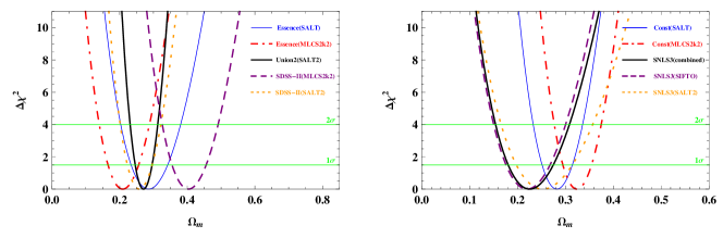
Figure 1: The constraints on the flat $\Lambda$CDM model from several popular SN Ia data sets compiled with different light-curve fitters. “Const” represents for the Constitution SN Ia sample.

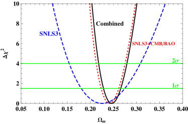
Figure 2: The constraints on the flat $\Lambda$CDM model. The blue dashed, red dotted and solid lines represent the results from SNLS3, SNLS3+CMB/BAO and SNL3+CMB/BAO+H(z), respectively.

This model is consistent with almost all observations. Fig. 1 shows a comparison of different SN Ia data constraints on the model parameter. From this Figure, we see that irrespective of whether SALT2, SALT, or SIFTO light curve fitter is used, different SN Ia samples give fairly consistent results. However, this is not the case when the MLCS2k2 light-curve fitter is considered, different SN Ia sets lead to notably different results. For example, the best fit values are $\Omega_{m}=0.209^{+0.059}_{-0.054}$ (ESSENCE), $\Omega_{m}=0.324^{+0.038}_{-0.036}$ (Constitution) and $\Omega_{m}=0.403^{+0.056}_{-0.059}$ (SDSS-II). In addition, as Sollerman et al. (2009), we also find that SDSS-II (SALT2) and SDSS-II (MLCS2k2) are clearly inconsistent. At the $95.4\%$ confidence level, the constraints from SDSS-II (SALT2) and SDSS-II (MLCS2k2) have no overlap. In Fig. 2, we give the constraints from SNLS3 with other cosmological probes, from which we find that the main constraints come from the SN Ia+CMB/BAO and the H(z) data set has little effect. Using SNLS3+CMB/BAO+H(z), we obtain $\Omega_{m}=0.245^{+0.026}_{-0.020}$ at the $68.3\%$ confidence level. Compared with the value of $\Omega_{m}=0.27\pm 0.04$ obtained by Davis et al. (2007) from ESSENCE+BAO+CMB, we find that SNLS3+CMB/BAO+H(z) yields a tighter constraint on $\Omega_{m}$.

3.2 Flat constant $w$

This model is obtained by assuming that dark energy has a constant equation of state parameter $w$. Thus the Friedmann equation can be expressed as:

$$H^{2}=H_{0}^{2}[\Omega_{m}(1+z)^{3}+(1-\Omega_{m})(1+z)^{3(1+w)}],$$ (11)

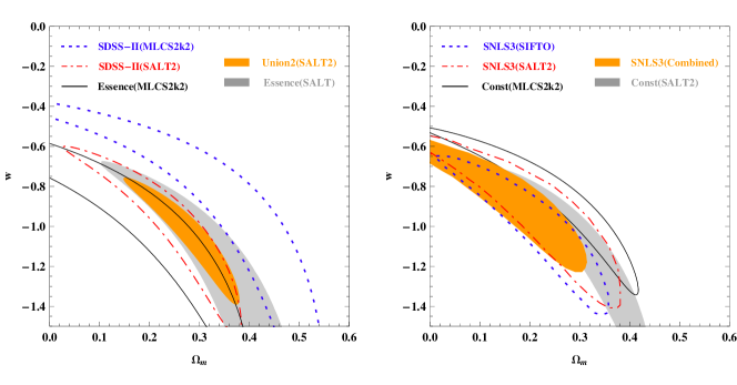
Figure 3: The $68.3\%$ contours for the flat constant $w$ model from several popular SN Ia data sets compiled with different light-curve fitters. “Const” represents for the Constitution SN Ia sample.

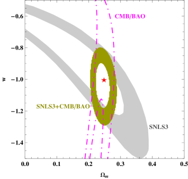
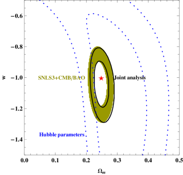
Figure 4: The $68.3\%$ and $95.4\%$ confidence level contours for the flat constant $w$ model. Left panel shows the constraints from SNLS3, CMB/BAO and their combination, and right panel is the case with the H(z) data included. The red star ($\Omega_{m}=0.25,~{}w=-1.0$) represents the $\Lambda$CDM with the best fit $\Omega_{m}$

which depends on two free parameters, $\Omega_{m}$ and $w$. Fig. 3 shows the constraints at the $68.3\%$ confidence level from different SN Ia samples, from which we find that, for all SN Ia data, especially for the SDSS-II, different light-curve fitters still affect the results. In the SDSS-II case, there exists an obvious inconsistency between SALT2 and MLCS2k2 since there is no overlap at the $68.3\%$ confidence level in this model. By fitting this model to the combined SNLS3 SN Ia, BAO/CMB and H(z) data, the $68.3\%$ constraints are $\Omega_{m}=0.248^{+0.024}_{-0.022}$ and $w=-1.039^{+0.135}_{-0.153}$. The contours of $\Omega_{m}$ and $w$ are plotted in Fig. 4. $w=-1$ is consistent with observations at the $68.3\%$ confidence level. As was the case for the $\Lambda$CDM, the H(z) has little effect on the derived cosmological parameters.

3.3 Flat varying $w$ (CPL)

The degrees of freedom of the cosmic model increase when we allow the dark energy equation of state to vary with the cosmic time. In this case, the Friedmann equation for a varying $w$ dark energy model is given by

$$H^{2}=H_{0}^{2}\bigg{\{}\Omega_{m}(1+z)^{3}+(1-\Omega_{m})\exp\bigg{[}3\int_{0}^{z}\frac{1+w(z^{\prime})}{1+z^{\prime}}dz^{\prime}\bigg{]}\bigg{\}}.$$ (12)

In this paper, we consider the popular CPL (Chevallier & Polarski, 2001; Linder, 2003) parametrization $w(z)=w_{0}+w_{1}z/(1+z)$. The above expression can then be simplified to

$$H^{2}=H_{0}^{2}\bigg{\{}\Omega_{m}(1+z)^{3}+(1-\Omega_{m})(1+z)^{3(1+w_{0}+w_{1})}\exp\bigg{[}-\frac{3w_{1}z}{1+z}\bigg{]}\bigg{\}}.$$ (13)

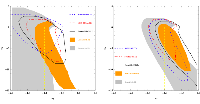
Figure 5: The marginalized $68.3\%$ contours of $w_{0}$ and $w_{1}$ in the flat CPL model from several popular SN Ia data sets which are compiled with different light-curve fitters. “Const” represents for the Constitution SN Ia sample.

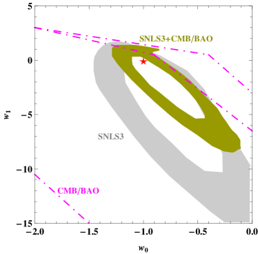
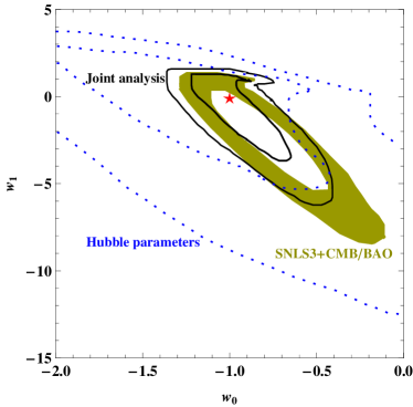
Figure 6: The marginalized $68.3\%$ and $95.4\%$ confidence level contours on $w_{0}-w_{1}$ for the varying $w$ model with the CPL parametrization. Left panel shows the constraints from SNLS3, CMB/BAO and their combination, and right panel is the case with the H(z) data included. The red star ($w_{0}=-1.0,~{}w_{1}=0.0$) represents the $\Lambda$CDM.

This model has been investigated by using SNLS3 in S11 and Li et al. (2011). In Fig. 5, we show the marginalized $68.3\%$ contours of $w_{0}$ and $w_{1}$ from different SN Ia data with different light-curve fitters. Consistent results are obtained and the tensions between different SN Ia sets and different light-curve fitters occurring in the $\Lambda$CDM and the constant $w$ model disappear when the CPL is considered. However, this tension improvements are probably simply due to the fact that this model is not well constrained by current data sets, especially the $w_{1}$ constraints are so bad. A combination of SNLS3+BAO/CMB+H(z) gives $\Omega_{m}=0.253^{+0.023}_{-0.020}$, $w_{0}=-1.007^{+0.187}_{-0.253}$, and $w_{1}=-0.344^{+1.144}_{-2.656}$ at the $68.3\%$ confidence level. The marginalized contours for $w_{1}$ and $w_{0}$ are plotted in Fig. 6. One can see that the $\Lambda$CDM ($w_{0}=-1.0,~{}w_{1}=0.0$) is included at the $68.3\%$ confidence level for all observational data sets, which are consistent with what obtained in S11 from SNLS3+SDSS DR7 LRGs+WMAP7+$H_{0}$.

3.4 Flat DGP model

The DGP model (Dvali et al., 2000), which accounts for the cosmic acceleration without dark energy, arises from a class of brane world theories in which gravity leaks out into the bulk at large distances. For a spatially flat case, the Friedmann equation in the DGP model can be expressed as

$$H^{2}=H_{0}^{2}[\sqrt{\Omega_{m}(1+z)^{3}+\Omega_{r_{c}}}+\sqrt{\Omega_{r_{c}}}]^{2},$$ (14)

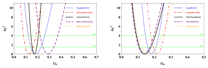
Figure 7: The constraints on the flat DGP model from several popular SN Ia data sets compiled with different light-curve fitters. “Const” represents for the Constitution SN Ia sample.

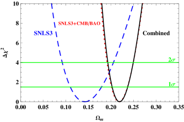
Figure 8: The constraints on the flat DGP model. The blue dashed, red dotted and solid lines represent the results from SNLS3, SNLS3+CMB/BAO and SNL3+CMB/BAO+H(z), respectively.

where $\Omega_{m}=1-2\sqrt{\Omega_{r_{c}}}$. The parameter $r_{c}$ represents the critical length scale beyond which gravity leaks out into the bulk and $\Omega_{r_{c}}$ is related to this critical length by $\Omega_{r_{c}}=1/(4r_{c}h_{0}^{2})$. The flat DGP model has the same number of free parameter as the $\Lambda$CDM. The constraints from different SN Ia samples are shown in Fig. 7. We obtain similar results to the $\Lambda$CDM for the DGP model, except that the latter favors a smaller $\Omega_{m}$. Fig. 8 shows the constraints on $\Omega_{m}$ from SNLS3, CMB/BAO and H(z) data, from which we find that the SNLS3 gives a very small value for $\Omega_{m}$ and this value becomes large when the CMB/BAO data are added. The combined SNLS3+CMB/BAO+H(z) gives $\Omega_{m}=0.219^{+0.022}_{-0.020}$, which is smaller than that obtained in Xu & Wang (2010); Liang & Zhu (2010) from other observations, where $\Omega_{m}=0.297^{+0.037}_{-0.039}$ and $0.285^{+0.252}_{-0.066}$, respectively.

It has been argued that the BAO data cannot be used to constrain the DGP model, since the details of structure formation are unclear in this model (Rydbeck et al., 2007). Moreover, it has been found that a tension between distance measures and horizon scale growth in the DGP exists and there is no way to alleviate it (Seahra & Hu, 2010; Song et al., 2007; Fang et al., 2008). With these caveats in mind, we still present the CMB/BAO constraints for the sake of completeness.

3.5 Flat Modified Polytropic Cardassian

The Cardassian model (Freese & Lewis, 2002) is based on a modified Friedmann equation in which an additional term $B\rho_{m}^{n}$ is added to the right hand side

$$H^{2}=\frac{8\pi G}{3}\rho_{m}+B\rho_{m}^{n},$$ (15)

where $\rho_{m}$ is the density of matter and $n$ is a dimensionless parameter. This equation can be rewritten as

$$H^{2}=\frac{8\pi G}{3}\rho_{m}\bigg{[}1+\bigg{(}\frac{\rho_{Card}}{\rho_{m}}\bigg{)}^{1-n}\bigg{]}.$$ (16)

This model reduces to the flat $\Lambda$CDM when $n=0$, and is related to the constant $w$ model by $n=1+w$. Therefore, the results for the original Cardassian model can be directly transcribed from those of section 3.2 and there is no need of additional fit for that model. Here, we consider a modified Cardassian model, the modified polytropic Cardassian model, in which the cosmic evolution is governed by (Wang et al., 2003):

$$H^{2}=\frac{8\pi G}{3}\rho_{m}\bigg{[}1+\bigg{(}\frac{\rho_{Card}}{\rho_{m}}\bigg{)}^{q(1-n)}\bigg{]}^{1/q}.$$ (17)

The above expression can be reexpressed as

$$H^{2}=H_{0}^{2}\bigg{\{}\Omega_{m}(1+z)^{3}\big{[}1+(\Omega_{m}^{-q}-1)(1+z)^{3q(n-1)}\big{]}^{1/q}\bigg{\}}.$$ (18)

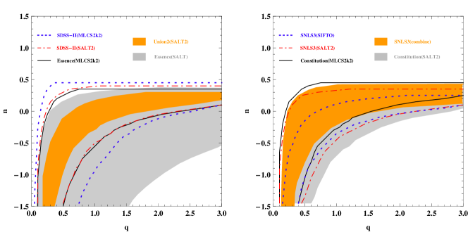
Figure 9: The marginalized $68.3\%$ contours for the flat modified polytropic Cardassian model from several popular SN Ia data sets which are compiled with different light-curve fitters.

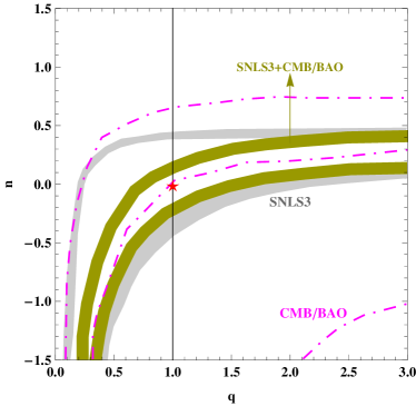
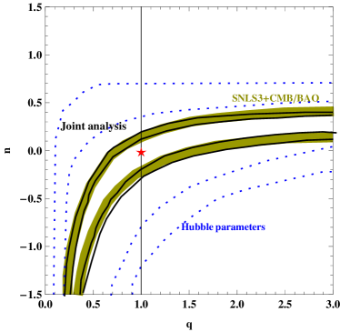
Figure 10: The marginalized $68.3\%$ and $95.4\%$ confidence level contours for the flat modified polytropic Cardassian model. Left panel shows the constraints from SNLS3, CMB/BAO and their combination, and right panel is the case of H(z) data included. The vertical line ($q=1.0$) represents the constant $w(=n-1)$ model, and the red star ($q=1.0,~{}n=0.0$) corresponds to the $\Lambda$CDM one.

$\Lambda$CDM is recovered for $q=1$ and $n=0$. The marginalized $68.3\%$ contours in the $q-n$ plane for different SN samples are shown in Fig. 9. As was the case for the varying $w$ CPL model, here we find that the differences between the constraints arising from different data and different light-curve fitters are negligible, which may also be due to the weak constraints on the model parameters from these observations. The constraint results from SNLS3 along with other data are shown in Fig. 10. The $\Lambda$CDM is well consistent with all observations at the $68.3\%$ confidence level. The combined analysis gives $\Omega_{m}=0.248^{+0.047}_{-0.013}$, $q=1.098^{+1.015}_{-0.465}$ and $n=0.014^{+0.364}_{-0.946}$, which is consistent with what given in Davis et al. (2007) (see Fig. 4) and in Wang & Wu (2009) ($\Omega_{m}=0.271^{+0.014}_{-0.015}$, $q=0.824^{+0.750}_{-0.622}$, $n=-0.091^{+0.331}_{-1.908}$).

3.6 Flat Generalized Chaplygin Gas

The Chaplygin gas model (Kamenshchik et al., 2001) unifies dark matter and dark energy by invoking a background fluid with an equation of state $p\propto\rho^{-\gamma}$, with $\gamma=1$ in the basic model. Here, we consider a generalization of this model (the Generalized Chaplygin Gas, or GCG model) by allowing $\gamma$ to take arbitrary, but constant, values (Bento et al., 2002). For the GCG, the Friedmann equation is

$$H^{2}=H_{0}^{2}\big{[}\Omega_{b}(1+z)^{3}+(1-\Omega_{b})\times\big{(}A_{s}+(1-A_{s})(1+z)^{3(1+\gamma)})^{\frac{1}{1+\gamma}}\big{]},$$ (19)

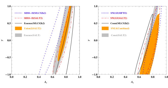
Figure 11: The constraints on the flat GCG model from several popular SN Ia data sets which are compiled with different light-curve fitters. “Const” represents for the Constitution SN Ia sample.

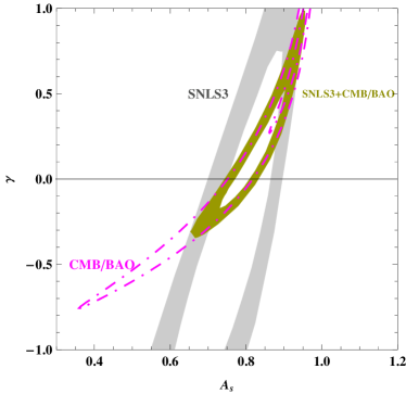
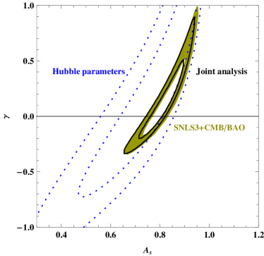
Figure 12: The $68.3\%$ and $95.4\%$ confidence level contours for the flat GCG model. Left panel shows the constraints from SNLS3, CMB/BAO and their combination, and right panel is the case with the H(z) data included. The horizontal line ($\gamma=0.0$) represents the standard cosmological constant model ($\Lambda$CDM) and $\gamma=1.0$ corresponds to the original Chaplygin gas one. The original Chaplygin gas model is ruled out by SNLS3+CMB/BAO and SNLS3+CMB/BAO+Hubble at the $95.4\%$ confidence level, while, except for the CMB/BAO data, the LCDM is allowed by observations at the $68.3\%$ confidence level.

where $\Omega_{b}$ is the present dimensionless density parameter of baryonic matter which is related to the effective matter density parameter by $\Omega_{m}=\Omega_{b}+(1-\Omega_{b})(1-A_{s})^{1/(1+\gamma)}$ and the WMAP7 observation gives $\Omega_{b}h^{2}=0.02246$  (Komatsu et al., 2011). Here $h$ is the Hubble constant in unit of $100~{}\mathrm{Km}\cdot\mathrm{s}^{-1}\cdot\mathrm{Mpc}^{-1}$ and we marginalize over it by using the Riess et al. (2011) $H_{0}$ prior. $A_{s}$ is a model parameter which relates the pressure $p$ and energy density $\rho$ of the background fluid: $A_{s}=p/\rho^{\gamma}$. $\gamma=0$ corresponds to the case of the cold dark matter plus a cosmological constant. The $68.3\%$ contours on $A_{s}$ and $\gamma$ from different SN data sets are shown in Fig. 11. The results are similar to the constant $w$ model. Inconsistency appears between SDSS-II (SALT2) and SDSS-II (MLCS2k2) and there is no overlap between them at the $68.3\%$ confidence level. The constraints from SNLS3 along with other cosmological probes are shown in Fig. 12. By fitting this model to the combined SNLS3 SN Ia, BAO/CMB and H(z) data, the constraints are $A_{s}=0.810^{+0.085}_{-0.095}$ and $\gamma=0.086^{+0.434}_{-0.286}$. We find that the standard Chaplygin gas model ($\gamma=1$) is ruled out by SNLS3+CMB/BAO and SNLS3+CMB/BAO+H(z) data at the $95.4\%$ confidence level, while the $\Lambda$CDM is consistent with them at the $68.3\%$ confidence level. This is consistent with the results of Davis et al. (2007); Liang et al. (2010); Lu et al. (2009); Wu & Yu (2007a, b).

4 MODEL TESTING USING MODEL SELECTION STATISTICS

In this section, we discuss the worth of models by applying model comparison statistics such as $\chi^{2}/dof$ ($dof$: degrees of freedom), goodness of fit (GoF), Akaike information criterion (AIC;, Akaike 1974) and Bayesian information criterion  (BIC;, Schwarz 1978). The $\chi^{2}/dof$ describes how well the model fits a set of observations. The GoF simply gives the probability of obtaining, by chance, a data set that is a worse fit to the model than the actual data, assuming the model is correct. It is defined as

$$\mathrm{GoF}=\Gamma(\nu/2,~{}\chi^{2}/2)/\Gamma(\nu/2),$$ (20)

where $\Gamma$ is the incomplete gamma function and $\nu$ is the number of degrees of freedom. For a family of models, the best fit one has a minimum $\chi^{2}/dof$ value, while it has a maximum value of GoF.

For a given data set, the candidate models may be ranked according to their AIC values, which can be calculated by

$$\mathrm{AIC}=-2\ln\mathcal{L}+2k$$ (21)

where $\mathcal{L}$ is the maximum likelihood, $k$ is the number of model parameters. Given a set of candidate models for the data, the one which has the minimum AIC value can be considered the best. Then the relative strength of evidence for each model can be judged by using the differences ($\Delta$AIC) between the AIC quantities of the rest of models and that of the best one. The models with $0\leq\Delta\mathrm{AIC}\leq 2$ are considered substantially supported, those where $4\leq\Delta\mathrm{AIC}\leq 7$ have less support, while models with $\Delta\mathrm{AIC}>10$ are essentially unsupported with respect to the best model (Szydlowski & Kurek, 2008).

The BIC, very similar to the AIC, is also a criterion for model selection among a finite set of models. It is defined as

$$\mathrm{BIC}=-2\ln\mathcal{L}+k\ln N$$ (22)

where $N$ is the number of data points used in the fit. The model which minimizes the BIC is the best fit one. As the AIC, the differences between the BIC of the rest of models and that of the best one ($\Delta$BIC) is used for the judgement of the model, that is, $0\leq\Delta\mathrm{BIC}\leq 2$ is considered as a weak, $2\leq\Delta\mathrm{BIC}\leq 6$ as a positive, $6\leq\Delta\mathrm{BIC}\leq 10$ as a strong and $\Delta\mathrm{BIC}>10$ as a very strong evidence favoring a better model (Liddle, 2004; Szydlowski & Kurek, 2008). Both the AIC and BIC penalize the case of adding the model parameter to increase the likelihood through the introduction of a penalty term, which depends on the number of parameters in the model. But the coefficients in this penalty term are different for the AIC and BIC. It should be noticed that in the limit of large data (large N) the AIC tends to favor models with more parameters while the BIC tends to penalize them (Parkinson et al., 2005).

The results for these model tests are shown in Table 2, 3, 4. From these tables, we find that, the DGP model is favored by the SNLS3 data alone. However, if additional constraints such as CMB/BAO and H(z) are included, this is no longer true, and the DGP model is disfavored by most criteria. Instead, the flat $\Lambda$CDM becomes preferred. The GCG and F$w$ are hardly distinguishable by most selection statistics and they become the favored non-standard models (excluding $\Lambda$CDM) when the CMB/BAO and H(z) are added. The variable $w$ (CPL) and Cardassian (MPC) models are penalized the most because of their large number of cosmological parameters.

5 Conclusion

In this paper, we compare the constraints from the enlarged first three years data of the Supernova Legacy Survey (SNLS3) with those from other SN Ia samples. Several popular SN Ia samples, such as ESSENCE, Union2, Constitution and SDSS-II are used and the effects of different light-curve fitters on results are considered. We also discuss the observational constraints from the SNLS3, together with other two cosmological probes, CMB/BAO and Hubble parameter versus redshift. The $\Lambda$CDM and five nonstandard cosmological models are considered. We find that, for models with fewer free parameters (F$\Lambda$, FDGP, F$w$ and FGCG; see Table 1), different SN Ia samples give fairly consistent results when analyzed with the SALT2, SALT, or SIFTO light-curve fitters, but this is not true when the MLCS2k2 light-curve fitter is used. Moreover, we find significant tension between SDSS-II sample results when analyzed with SALT2 or MLCS2k2, as noted in Sollerman et al. (2009). The inconsistencies between different samples and different light-curve fitters seem to be reduced for models with more free parameters (FCPL and FMPC). This improvement may be ascribed to the fact that current observational data has a weak constraint on the model parameters.

By combining the SNLS3 with CMB/BAO and Hubble parameter versus redshift data, we find that, except for the flat varying $w$ model, the main constraints on model parameters come from the SNLS3+CMB/BAO and the H(z) data has little effect. Moreover, we study the worth of models by applying model comparison statistics such as $\chi^{2}/dof$, goodness of fit (GoF), Akaike information criterion and Bayesian information criterion. We find that the DGP model is the best one for SNLS3 alone while the flat $\Lambda$CDM is preferred when the CMB/BAO or H(z) data is included. When only the nonstandard models are considered ($\Lambda$CDM is excluded), the GCG and F$w$ are preferred by both SNLS3+CMB/BAO and SNLS3+CMB/BAO+H(z) data. These results are independent of the test methods, that is, different test methods give consistent conclusions. Our results are slightly different from that of the analysis of the SDSS-II (Sollerman et al., 2009) and ESSENCE SN Ia data (Davis et al., 2007). In Sollerman et al. (2009), both SDSS-II (MLCS2k2) and SDSS-II (MLCS2k2) plus CMB/BAO prefer the DGP model, while, once the SDSS-II (SALT2) is used, the $\Lambda$CDM is always the best fit one. In Davis et al. (2007), the combination of ESSENCE (MLCS2k2), BAO, and CMB favors the $\Lambda$CDM. Finally, the FCPL and FMPC suffer in BIC test due to the extra model parameters, which agrees with the conclusions in (Davis et al., 2007; Sollerman et al., 2009).

Model                      $\chi^{2}/dof$                  GoF(%)           $\Delta$AIC            $\Delta$BIC
FDGP…..          419.464/472(0.8887)           96.04              0.00              0.00
F$\Lambda$………           419.691/472(0.8892)           95.98              0.23              0.23
F$w$………           419.282/471(0.8902)           95.81              1.82              5.98
FGCG….           419.342/471(0.8903)           95.79              1.88              6.04
FMPC….           418.472/470(0.8904)           95.77              3.01              11.32
FCPL…..           418.664/470(0.8908)           95.71              3.20              11.51

Table 2: Summary of the model test results for the SNLS3. The models are listed in the increasing order of the $\Delta$AIC values (please refer to Table 1 for the definitions of the model acronyms). When only the SNLS3 is considered, the flat DGP is preferred.

Model                      $\chi^{2}/dof$                  GoF(%)           $\Delta$AIC            $\Delta$BIC
F$\Lambda$………           422.741/474(0.8919)           95.61              0.00              0.00
FGCG….           422.487/473(0.8932)           95.38              1.75              5.91
F$w$………           422.603/473(0.8935)           95.34              1.86              6.02
FCPL…..           421.124/472(0.8922)           95.52              2.38              10.71
FMPC….           421.213/472(0.8924)           95.49              2.47              10.79
FDGP…..           429.995/474(0.9072)           92.71             7.25               7.25

Table 3: Summary of the model test results for SNLS3+CMB/BAO. The models are listed in the increasing order of the $\Delta$AIC values (please refer to Table 1 for the definitions of the model acronyms). When the additional CMB/BAO is included, the flat DGP is disfavored and the flat $\Lambda$CDM becomes preferred.

Model                      $\chi^{2}/dof$                  GoF(%)           $\Delta$AIC            $\Delta$BIC
F$\Lambda$………           436.106/488(0.8937)           95.57              0.00              0.00
FGCG….           435.931/487(0.8951)           95.31              1.83              6.02
F$w$………           435.938/487(0.8951)           95.31              1.83              6.02
FMPC….           435.656/486(0.8964)           95.08              3.55              11.93
FCPL…..           435.900/486(0.8969)           94.99              3.79              12.18
FDGP…..           443.030/488(0.9078)           92.85              6.92               6.92

Table 4: Summary of the model test results for SNLS3+CMB/BAO+H(z). The models are listed in the increasing order of the $\Delta$AIC values (please refer to Table 1 for the definitions of the model acronyms). When the additional H(z) is included, the flat DGP is still disfavored and the flat $\Lambda$CDM remains preferred.

References

- AIC; (Akaike 1974) Akaike, H. 1974, IEEE Trans. Automatic Control, 19, 716
- Amanullah et al. (2010) Amanullah, R., et al. 2010, Astrophys. J., 716, 712
- Astier et al. (2006) Astier, P., et al. 2006, A&A, 447, 31
- Bengochea (2011) Bengochea, G. R. 2011, Phys. Lett. B, 696, 5
- Bento et al. (2002) Bento, M. C., Bertolami, O., & Sen, A. A. 2002, Phys. Rev. D, 66, 043507
- Bueno Sancheza et al. (2009) Bueno Sancheza, J. C., Nesserisb, S. and Perivolaropoulos, L. 2009, arXiv:0908.2636
- Chevallier & Polarski (2001) Chevallier, M., and Polarski, D. 2001, Int. J. Mod. Phys. D, 10, 213
- Conley et al. (2008) Conley, A., et al. 2008, Astrophys. J., 681, 482
- Conley et al. (2011, hereafter C11) Conley, A., et al. 2011, ApJS, 192, 1
- Davis et al. (2007) Davis, T. M., et al. 2007, Astrophys. J., 666, 716
- Dvali et al. (2000) Dvali, G., Gabadadze, G., & Porrati, M. 2000, Phys. Lett. B, 484, 112
- Fang et al. (2008) Fang, W., Wang, S., Hu. W., Haiman, H., Hui, L. and May, M. 2008, Phys. Rev. D, 78, 103509
- Freese & Lewis (2002) Freese, K., & Lewis, M. 2002, Phys. Lett. B, 540, 1
- Gaztanaga et al. (2009) Gaztanaga, E., et al. 2009, Mon. Not. Roy. Astron. Soc., 399, 1663
- Guy et al. (2005) Guy, J., Astier, P., Nobili, S., Regnault, N., & Pain, R. 2005, A&A, 443, 781
- Guy et al. (2007) Guy, J., et al. 2007, A&A, 466, 11
- Guy et al. (2010, hereafter G10) Guy, J., et al. 2010, A&A, 523, A7
- Hicken et al. (2009) Hicken, M., et al. 2009, Astrophys. J., 700, 1097
- Jha (2002) Jha, S. 2002, PhD thesis, University of Washington
- Jha et al. (2007) Jha, S., Riess, A. G., & Kirshner, R. P. 2007, Astrophys. J., 659, 122
- Kamenshchik et al. (2001) Kamenshchik, A., Moschella, U., & Pasquier, V. 2001, Phys. Lett. B, 511, 265
- Kessler et al. (2009) Kessler, R., et al. 2009, ApJS, 185, 32
- Komatsu et al. (2009) Komatsu, E., et al. 2009, ApJS, 180, 330
- Komatsu et al. (2011) Komatsu, E., et al. 2011, ApJS, 192, 18
- Li et al. (2011) Li, X. D., et al. 2011, JCAP07(2011)011
- Liang & Zhu (2010) Liang, N. and Zhu, Z. 2010, arXiv:1010.2681
- Liang et al. (2010) Liang, N., Xu, L. and Zhu, Z. 2010, arXiv:1009.6059
- Liddle (2004) Liddle, A. R. 2004, Mon. Not. Roy. Astron. Soc., 351, L49
- Linder (2003) Linder, E. V. 2003, Phys. Rev. Lett., 90, 091301
- Lu et al. (2009) Lu, J., Gui, Y., Xu L. 2009, Eur. Phys. J. C, 63, 349
- Parkinson et al. (2005) Parkinson, D., Tsujikawa, S., Bassett, B. A., Amendola, L. 2005, Phys.Rev. D, 71, 063524
- Phillips (1993) Phillips, M. M. 1993, Astrophys. J., 413, L105
- Percival et al. (2007) Percival, W. J., et al. 2007, Mon. Not. Roy. Astron. Soc., 381, 1053
- Percival et al. (2009) Percival, W. J., et al. 2009, Mon. Not. Roy. Astron. Soc., 401, 2148
- Perlmutter et al. (1999) Perlmutter, S., et al. 1999, Astron. J., 617, 565
- Rydbeck et al. (2007) Rydbeck, R., Fairbairn and Goobar, A. 2007, JCAP003(2007)0705
- Regnault et al. (2009) Regnault, N., et al. 2009, A&A, 506, 999
- Riess et al. (1995) Riess, A. G., Press, W. H., & Kirshner, R. P. 1995, Astron. J., 438, L17
- Riess et al. (1998) Riess, A. G., et al. 1998, Astron. J., 116, 1009
- Riess et al. (2011) Riess, A. G., et al. 2011, Astrophys. J., 730, 119
- BIC; (Schwarz 1978) Schwarz, G. 1978, Ann. Stat., 6, 461
- Seahra & Hu (2010) Seahra, S. S. and Hu, W. 2010, Phys. Rev. D, 82, 124015
- Simon et al. (2005) Simon, J., Verde, L., and Jimenez, J. 2005, Phys. Rev. D, 71, 123001
- Sollerman et al. (2009) Sollerman, J., et al. 2009, Astrophys. J., 703, 1374
- Song et al. (2007) Song, Y. S., Sawicki, I. and Hu W. 2007, Phys. Rev. D, 75, 064003
- Stern et al. (2010) Stern, D., et al. 2010, JCAP02(2010)008
- Sullivan et al. (2005) Sullivan, M., et al. 2005, ASP Conf. Ser., 342, 466
- Sullivan et al. (2010) Sullivan, M., et al. 2010, Mon. Not. Roy. Astron. Soc., 406, 782
- Sullivan et al. (2011, hereafter S11) Sullivan, M., et al. 2011, Astrophys. J., 737, 102
- Szydlowski & Kurek (2008) Szydlowski, M., and Kurek, A. 2008, arxiv:0801.0638
- Wang & Wu (2009) Wang, T. and Wu, P. 2009, Phys. Lett. B, 678, 32
- Wang et al. (2003) Wang, Y., Freese, K., Gondolo, P., & Lewis, M. 2003, Astrophys. J., 594, 25
- Wood-Vasey et al. (2007) Wood-Vasey, W. M., et al. 2007, Astrophys. J., 666, 694
- Wu & Yu (2007a) Wu, P. X., and Yu, H. W. 2007, Phys. Lett. B, 644, 16
- Wu & Yu (2007b) Wu, P. X., and Yu, H. W. 2007, Astrophys . J., 658, 663
- Xu & Wang (2010) Xu, L., Wang, Y. 2010, Phys. Rev. D, 82, 043503