Computing the lower and upper bounds of Laplace eigenvalue problem: by combining conforming and nonconforming finite element methods

Abstract.

This article is devoted to computing the lower and upper bounds of the Laplace eigenvalue problem. By using the special nonconforming finite elements, i.e., enriched Crouzeix-Raviart element and extension $Q_{1}^{\rm rot}$, we get the lower bound of the eigenvalue. Additionally, we also use conforming finite elements to do the postprocessing to get the upper bound of the eigenvalue. The postprocessing method need only to solve the corresponding source problems and a small eigenvalue problem if higher order postprocessing method is implemented. Thus, we can obtain the lower and upper bounds of the eigenvalues simultaneously by solving eigenvalue problem only once. Some numerical results are also presented to validate our theoretical analysis.

1. Introduction

The eigenvalue problems are important, which appears in many fields, such as quantum mechanics, fluid mechanics, stochastic process and etc.Thus, a fundamental work is to find the eigenvalues of partial differential equations. From last century, abundant works are dedicated to this topic.

Feng in his famous paper [6] cites the pioneer work of Pólya in computing the upper bound of Laplace eigenvalue problem. And based on the minimum-maximal principle discovered by Rayleigh, Poincaré, Courant and Fischer ect., any conforming finite element method will give the upper bound (see Strang and Fix [18]). Nevertheless, to the lower bound aspect, until 1979, Rannacher [17] gives some numerical results for plate problem.

And then there is few work on analysis of the lower bound for a long time. Hu, Huang and Shen [7] get the lower bound of Laplace equation by conforming linear and bilinear elements together with the mass lumping method. Inspired by the minimum-maximal principle, people try to find the lower bound with the nonconforming element methods. Recently, a series of works make progress in this aspect, e.g. Lin and Lin [11] use the asymptotic expansion skill to compute the eigenvalues by nonconforming finite element method; also see the numerical reports of Liu and Liu [15], Liu and Yan [16], and the work of Lin, Huang and Li [10]. Another way by Armentano and Durán [1] is to use another kind of expansion method to get the lower bound, which is of less restriction to the smoothness of eigenfunctions compared with the asymptotic expansion skill. Also see the follow-up works by Li [9], Lin [13], Yang [21].

Inspired by these works, this article propose a method to obtain the lower and upper bounds of the eigenvalue simultaneously which only need to solve the eigenvalue problem once and additional auxiliary source problem. Our method can be described as follows: (1) solve the eigenvalue problem by some nonconforming finite element; (2) solve an additional auxiliary source problem in an conforming finite element space. Since we obtain not only lower bound but also upper bound of the eigenvalue, we can give the accurate error of the eigenvalue approximations. Compared with the existed literature, this note contributes on the following aspects:

• The assumption of the lower bound in [1] needs an critical assumption that: $|u-u_{h}|_{1}\geq Ch^{\gamma}$, $\gamma<1$, which promise itself be the dominant term in the expansion. By our recent result of lower bound of convergence rate by finite element method, we get rid of this constrain.

• A new application of the correction method of eigenvalue problem is proposed to obtain the lower and upper bounds of the eigenvalues by solving the eigenvalue problem once and an additional source problem.

• By using higher order conforming finite element to do the correction in a new way, we also prove the upper bound of the corrected eigenvalue approximations.

• After calculating upper and lower bounds simultaneously, we can find how much accuracy we have actually achieved (an accurate a posteriori error estimate).

For simplicity, we only discuss the problem in $\mathcal{R}^{2}$, but the methods and results here can be easily extended to the case $\mathcal{R}^{3}$. In this paper, we will use the standard notation of Sobolev spaces ([18]). The outline of the paper is as follows. In Section 2, some preliminaries and notation are introduced. The weak form of the Laplace eigenvalue problem and its corresponding discrete form is stated. In Section 3, we will give the results about the lower bound with nonconforming finite elements. Section 4 is devoted to analyzing the upper bound of the eigenvalue by postprocessing with the lowest order conforming finite element methods. In section 5, another type of postprocessing method is proposed to obtain not only higher order accuracy but also upper bound approximation of the eigenvalues. Some numerical results are presented in section 6 to test our theoretical results and some concluding remarks are given in the last section.

2. The eigenvalue problem

In this paper we are concerned with the Laplace eigenvalue problem:

Find $(\lambda,u)$ such that

(2.1) $$\left\{\begin{array}[]{rcl}-\triangle u&=&\lambda u,\quad\text{in }\Omega,\\ u&=&0,\quad\ \ \text{on }\partial\Omega,\\ \int_{\Omega}u^{2}dxdy&=&1,\end{array}\right.$$

where $\Omega$ is a bounded domain in $\mathcal{R}^{2}$ with continuous Lipschitz boundary $\partial\Omega$ .

The variational problem associated with (2.1) is given by:

Find $u\in V:=H_{0}^{1}(\Omega)$ and $\lambda\in\mathcal{R}$ such that $b(u,u)=1$ and

(2.2) $$a(u,v)=\lambda b(u,v),\quad\forall v\in V,$$

where

$$a(u,v)=\int_{\Omega}\nabla u\cdot\nabla vdxdy\ \ {\rm and}\ \ \ b(u,v)=\int_{\Omega}uvdxdy.$$

From [3], we know that the Lapalce eigenvalue problem has a positive eigenvalue sequence $\{\lambda_{j}\}$ with

$$0<\lambda_{1}\leq\lambda_{2}\leq\cdots\leq\lambda_{k}\leq\cdots,\quad\lim\limits_{k\rightarrow\infty}\lambda_{k}=\infty,$$

and the corresponding eigenfunction sequence $\{u_{j}\}$

$$u_{1},u_{2},\cdots,u_{k},\cdots,$$

with the property $b(u_{i},u_{j})=\delta_{ij}$.

From the result in [3], the Rayleigh quotient is defined by

$$R(u):=\frac{a(u,u)}{b(u,u)}=\lambda.$$

We define the discrete finite element method to solve the problem (2.3). $\mathcal{T}_{h}$ is a quasi-uniform triangulation. Based on this partition, $\mathcal{E}_{h}$ denotes the set of all edges in partition $\mathcal{T}_{h}$. The finite element space $V_{h}$ is the corresponding finite element space to the partition, i.e. $V^{NC}_{h}\nsubseteq V$ as a nonconforming space and $V^{C}_{h}\subset V$ a conforming space.

In the rest of this paper, the finite element space $V_{h}$ can be $V_{h}^{C}$ or $V_{h}^{NC}$. The finite element approximation of (2.2) is defined as follows:

Find $(\lambda_{h},u_{h})\in\mathcal{R}\times V_{h}$ such that $b(u_{h},u_{h})=1$ and

(2.3) $$a_{h}(u_{h},v_{h})=\lambda_{h}b(u_{h},v_{h}),\quad\forall v_{h}\in V_{h},$$

where the bilinear form $a_{h}(\cdot,\cdot)$ coincides with $a(\cdot,\cdot)$ in conforming finite element, or a elementwise representation of $a(\cdot,\cdot)$ in nonconforming situation, e.g.

$$a_{h}(u_{h},v_{h})=\sum\limits_{K\in\mathcal{T}_{h}}\int_{k}\nabla u_{h}\cdot\nabla v_{h}dxdy.$$

Obviously, the bilinear form for conforming situation can also be presented as this form. It is easy to see that for both situation, the bilinear are $V_{h}-$elliptic. Thus, we define the norm on $V_{h}+V$ by

$$\|v\|_{a,h}^{2} = a_{h}(v,v),\ \ \ \ {\rm for}\ v\in V_{h}^{NC},$$

and

$$\|v\|_{a}^{2} = a(v,v),\ \ \ \ \ \ {\rm for}\ v\in V+V_{h}^{C}.$$

For both conforming and nonconforming situations, the Rayleigh quotient holds for the eigenvalue $\lambda_{h}$

$$R(u_{h})=\frac{a_{h}(u_{h},u_{h})}{b(u_{h},u_{h})}=\lambda_{h}.$$

Similarly, the discrete eigenvalues problem (2.3) has also an eigenvalue sequence $\{\lambda_{j,h}\}$ with

$$0<\lambda_{1,h}\leq\lambda_{2,h}\leq\cdots\leq\lambda_{N,h},$$

and the corresponding discrete eigenfunction sequence $\{u_{k,h}\}$

$$u_{1,h},u_{2,h},\cdots,u_{k,h},\cdots,u_{N,h}$$

with the property $b(u_{i,h},u_{j,h})=\delta_{ij},1\leq i,j\leq N_{h}$ ($N_{h}$ is the dimension of $V_{h}$).

We cite here the classical result about eigenvalue: minimum-maximum principle. Let $\lambda_{j}$ be the $j-$th eigenvalue of (2.2) and $\lambda_{j,h}$ be the $j-$th eigenvalue of (2.3), respectively. Arranging them by increasing order, then we have ([3])

(2.4) $$\lambda_{j}=\min\limits_{V_{j}\subset V,\dim V_{j}=j}\max\limits_{v\in V_{j}}R(v),\quad\lambda_{j,h}=\min\limits_{V_{j}\subset V_{h},\dim V_{j}=j}\max\limits_{v\in V_{j}}R(v).$$

Since the convergence of the finite element approximation to the eigenvalue problem depends on the regularity of the original eigenvalue problem, here we assume that the regularity of the eigenfunction $u\in H^{1+\gamma}(\Omega)$ with $0<\gamma\leq 1$ which is decided by the largest inner angle of the boundary $\partial\Omega$.

For the eigenvalue problem, we have the following basic expansion from [1], and has been extensively used in [13, 20, 21].

Lemma 2.1.

Suppose $(\lambda,u)$ is the eigenpair of the original problem (2.1), $(\lambda_{h},u_{h})\in\mathcal{R}\times V_{h}$ is the eigenpair of the discrete problem (2.3), we have the following expansion

$$\lambda-\lambda_{h}=\|u-u_{h}\|_{a,h}^{2}-\lambda_{h}\|v_{h}-u_{h}\|_{b}^{2}$$

(2.5) $$\ +\lambda_{h}(\|v_{h}\|_{b}^{2}-\|u\|_{b}^{2})+2a_{h}(u-v_{h},u_{h}),\quad\forall v_{h}\in V_{h}.$$

3. Lower bound with nonconform finite element methods

In this paper, we are concerned with two types of nonconforming finite elements: Enriched Crouzeix-Raviart (ECR) ([8, 13]) and Extension $Q_{1}^{\rm rot}$ ($EQ_{1}^{\rm rot}$) ([12]) for triangle and rectangle partitions, respectively.

• ECR element is defined on the triangle partition and

  $$V_{h}^{NC}:= \Big{\{}v\in L^{2}({\it\Omega}):v|_{K}\in{\rm span}\{1,x,y,x^{2}+y^{2}\},\int_{\ell}v|_{K_{1}}{\rm d}s=\int_{\ell}v|_{K_{2}}{\rm d}s,$$

  (3.1) $$\hskip 28.45274pt\text{ when }K_{1}\cap K_{2}=\ell\in\mathcal{E}_{h},\ \text{and }\int_{\ell}v|_{K}{\rm d}s=0,\text{ if }K\cap\partial{\it\Omega}=\ell\Big{\}},$$

  where $K,\ K_{1},\ K_{2}\in\mathcal{T}_{h}$.

• On the rectangle partition, $EQ_{1}^{\rm rot}$ is employed defined by

  $$V_{h}^{NC}:= \Big{\{}v\in L^{2}(\Omega):v|_{K}\in{\rm span}\{1,x,y,x^{2},y^{2}\},\int_{\ell}v|_{K_{1}}ds=\int_{\ell}v|_{K_{2}}ds,$$

  (3.2) $$\hskip 28.45274pt\text{if }K_{1}\cap K_{2}=\ell,\text{ and }\int_{\ell}v|_{K}ds=0,\text{ if}\ K\cap\partial\Omega=\ell\Big{\}},$$

  where $K,\ K_{1},\ K_{2}\in\mathcal{T}_{h}$.

From [8] and [13], the following basic error estimates for the two nonconforming finite elements hold

(3.3) $$|\lambda-\lambda_{h}| \leq Ch^{2\gamma}\|{u}\|_{1+\gamma}^{2},$$

(3.4) $$\|u-u_{h}\|_{a,h} \leq Ch^{\gamma}\|u\|_{1+\gamma}\ ,$$

(3.5) $$\|u-u_{h}\|_{b} \leq Ch^{\gamma}\|u-u_{h}\|_{a,h}\leq Ch^{2\gamma}\|u\|_{1+\gamma}.$$

The interpolation operator corresponding to ECR and $EQ_{1}^{\rm rot}$ can be defined in the same way:

(3.6) $$\int_{\ell}(u-{\it\Pi}_{h}u)ds = 0,\ \ \ \ \forall\ell\in\mathcal{E}_{h},$$

(3.7) $$\int_{K}(u-{\it\Pi}_{h}u){\rm d}K = 0,\ \ \ \ \forall K\in\mathcal{T}_{h},$$

Lemma 3.1.

(See [13]) For the ECR and $EQ_{1}^{\rm rot}$ elements, the interpolation operator satisfies:

$$\|u-{\it\Pi}_{h}u\|_{b}+h\|u-{\it\Pi}_{h}u\|_{a,h}\leq Ch^{1+\gamma}\|u\|_{1+\gamma},$$

for any $u\in H^{1+\gamma}(\Omega)$.

Lemma 3.2.

With the interpolation defined above, for any $u\in V$, we have the following results

(3.8) $$a_{h}(u-\it\Pi_{h}u,\it\Pi_{h}u)=0,$$

(3.9) $$\|\it\Pi_{h}u\|_{a,h}\leq C\|u\|_{a},$$

(3.10) $$\|u-\it\Pi_{h}u\|_{b}\leq Ch\|u-\it\Pi_{h}u\|_{a,h},$$

(3.11) $$\|u-\it\Pi_{h}u\|_{b}\leq Ch\|u-u_{h}\|_{a,h}.$$

Proof.

Here we only give the proof for the ECR element and the one for $EQ_{1}^{\rm rot}$ is almost the same.

Integrating by parts, we have

$$a_{h}(u-\it\Pi_{h}u,\it\Pi_{h}u)=\sum_{K\in\mathcal{T}_{h}}\big{[}\int_{K}(u-\it\Pi_{h}u)\triangle\Pi_{h}udxdy+\int_{\partial K}(u-\it\Pi_{h}u)(\nabla\it\Pi_{h}u)\cdot\textbf{n}ds\big{]}.$$

Since $\it\Pi_{h}u\in V^{NC}_{h}$

$$\triangle\it\Pi_{h}u=const.$$

From the definition of the face interpolation, the following equality holds

$$\int_{K}(u-\it\Pi_{h}u)\triangle\Pi_{h}udxdy=0.$$

For any $\ell\in\partial K$ can denoted by the linear function $y=kx+m$, then the normal direction corresponding to this edge is $\mathbf{n}=\frac{1}{\sqrt{1+k^{2}}}(\pm{k,-1})$. Thus suppose $\it\Pi_{h}u=a+bx+cy+d(x^{2}+y^{2})$, we have

$$(\nabla\it\Pi_{h}u)\cdot\mathbf{n} = \pm(b+2dx,c+2dy)\frac{1}{\sqrt{1+k^{2}}}(k,-1)^{T}$$

$$= \pm\frac{1}{\sqrt{1+k^{2}}}(bk-c-2dm)=const.$$

From the definition of the interpolation, we have

$$\int_{\ell}(u-\it\Pi_{h}u)(\nabla\it\Pi_{h}u)\cdot\mathbf{n}ds=0.$$

So

$$a_{h}(u-\it\Pi_{h}u,\it\Pi_{h}u)=0.$$

From (3.8), we can obtain

$$a_{h}(\it\Pi_{h}u,\Pi_{h}u)=a_{h}(u,\it\Pi_{h}u)\leq\|\it\Pi_{h}u\|_{a,h}\|u\|_{a,h}.$$

Canceling the term $\|\it\Pi_{h}u\|_{a,h}$ leads to (3.9).

Defining $\Pi_{0}$ be the piecewise constant interpolation, we have

$$\|u-\it\Pi_{h}u\|^{2}_{b} = b(u-\it\Pi_{h}u,u-\it\Pi_{h}u-\Pi_{0}(u-\it\Pi_{h}u))$$

$$\leq \|u-\it\Pi_{h}u\|_{b}\|u-\it\Pi_{h}u-\Pi_{0}(u-\it\Pi_{h}u)\|_{b}$$

$$\leq C\|u-\it\Pi_{h}u\|_{b}h\|u-\it\Pi_{h}u\|_{a,h}.$$

It means we arrive the result (3.10).

For the last inequality, from (3.9) and (3.10), we have following equality

$$\|u-\it\Pi_{h}u\|_{b}\leq Ch\|u-\it\Pi_{h}u\|_{a,h}\leq Ch(\|u-u_{h}\|_{a,h}+\|u_{h}-\it\Pi_{h}u\|_{a,h})$$

$$=Ch\big{(}\|u-u_{h}\|_{a,h}+\|\Pi_{h}u_{h}-\it\Pi_{h}u\|_{a,h}\big{)}\leq Ch\|u-u_{h}\|_{a,h}.$$

Thus, we get (3.11). ∎

Lemma 3.3.

([14, Section 3]) If we solve the eigenvalue problem (2.2) by $Q_{1}^{\rm rot}$, ECR, bilinear or linear elements, the following lower bound for the convergence rate holds

(3.12) $$\|u-u_{h}\|_{a,h} \geq Ch.$$

Theorem 3.4.

Let $\lambda_{j}$ and $\lambda_{j,h}$ be the $j$-th exact eigenvalue and its corresponding numerical approximation by ECR or $EQ_{1}^{\rm rot}$ element. Assume $u_{j}\in H^{1+\gamma}(\Omega)$ with $0<\gamma\leq 1$. When $h$ is small enough, we have

(3.13) $$0\leq\lambda_{j}-\lambda_{j,h}\leq Ch^{2\gamma}\|u\|_{1+\gamma}^{2}.$$

Proof.

The result for ECR and $EQ_{1}^{\rm rot}$ elements can be proved in the uniform way. We choose $v_{j,h}={\it\Pi_{h}}u_{j}$ in Lemma 2.1. For the second term in (2.1), from Lemma 3.2, we have

$$\|u_{j,h}-\it\Pi_{h}u_{j}\|^{2}_{b}\leq Ch^{2}\|u_{j}-u_{j,h}\|^{2}_{a,h}.$$

For the third term in (2.1), from (3.11), we have

$$\|v_{j,h}\|_{b}^{2}-\|u_{j}\|_{b}^{2} = ({\it\Pi_{h}}u_{j}-u_{j},{\it\Pi_{h}}u_{j}+u_{j})$$

$$= \big{(}{\it\Pi_{h}}u_{j}-u_{j},({\it\Pi_{h}}u_{j,h}+u_{j})-{\it\Pi_{0}}({\it\Pi_{h}}u_{j,h}+u_{j})\big{)}$$

$$\leq Ch\|{\it\Pi_{h}}u_{j}-u_{j}\|_{b}\leq Ch^{2}\|u_{j}-u_{j,h}\|_{a,h},$$

where $\Pi_{0}$ denotes the piecewise constant interpolation. Together with (3.8) and Lemma 3.3, the first term will be the dominant term in (2.5) and then (3.13) can be derived. ∎

4. Upper bound with linear conforming element

4.1. Upper bound by direct use of linear conforming element

Due to the minimum-maximal principle (2.4), by using conforming finite element, we can get the upper bound naturally. Here we use the lowest order conforming element for both triangle and rectangle partitions, respectively

• On the triangle partition, we use the linear element defined as below:

  (4.1) $$V_{h}^{C}:= \Big{\{}v\in C^{0}({\it\Omega}):v|_{K}\in{\rm span}\{1,x,y\}\Big{\}}\cap H^{1}_{0}(\Omega).$$

• On the rectangle partition, the bilinear element is employed here:

  (4.2) $$V_{h}^{C}:= \Big{\{}v\in C^{0}({\it\Omega}):v|_{K}\in{\rm span}\{1,x,y,xy\}\Big{\}}\cap H^{1}_{0}(\Omega).$$

In the conforming finite element space $V_{h}^{C}$, we can define the corresponding discrete eigenvalue problem:

Find ($\overline{\lambda}_{h},\overline{u}_{h}$)$\in\mathcal{R}\times V_{h}^{C}$ such that $b(\overline{u}_{h},\overline{u}_{h})=1$ and

(4.3) $$a(\overline{u}_{h},\overline{v}_{h})=\overline{\lambda}_{h}(\overline{u}_{h},\overline{v}_{h}),\quad\forall\overline{v}_{h}\in V_{h}^{C}.$$

From [3], the basic estimates about approximation errors exist

(4.4) $$0\leq\overline{\lambda}_{h}-\lambda \leq Ch^{2\gamma}\|{u}\|_{1+\gamma}^{2},$$

(4.5) $$\|u-\overline{u}_{h}\|_{a,h} \leq Ch^{\gamma}\|u\|_{1+\gamma}\ ,$$

(4.6) $$\|u-\overline{u}_{h}\|_{b} \leq Ch^{2\gamma}\|u\|_{1+\gamma}.$$

So by (4.4), (3.3) and Theorem 3.4, we have the following estimate between conforming and nonconforming eigenvalue approximations:

(4.7) $$0\leq\lambda-\lambda_{h} \leq Ch^{2\gamma}\|{u}\|_{1+\gamma}^{2},$$

(4.8) $$0\leq\overline{\lambda}_{h}-\lambda \leq Ch^{2\gamma}\|{u}\|_{1+\gamma}^{2},$$

(4.9) $$0\leq\overline{\lambda}_{h}-\lambda_{h} \leq Ch^{2\gamma}\|{u}\|_{1+\gamma}^{2}.$$

4.2. Upper bound by postprocess

The results (4.7)-(4.9) are very interesting and useful. Especially, (4.9) can give a guaranteed error for the current numerical approximations. Unfortunately, in order to get (4.9), we need to solve the eigenvalue problem twice, one with nonconforming and the other with conforming elements, which is always difficult since solving eigenvalue problem need much more computation than solving the corresponding source problems. So, in this subsection we give a postprocessing method to obtain the upper bound eigenvalue approximation without solving eigenvalue problem but only need to solve a source problem.

After obtaining the eigenpair approximation $(\lambda_{h},u_{h})\in\mathcal{R}\times V_{h}^{NC}$ by the nonconforming finite element, we put them as the right hand side of an auxiliary source Laplace problem. Then we utilize conforming finite element method to solve this problem which is defined as follows:

(4.10) $$a(\widehat{u}_{h},\widehat{v}_{h})=\lambda_{h}b(u_{h},\widehat{v}_{h}),\ \quad\forall\widehat{v}_{h}\in V_{h}^{C}$$

After obtaining $\widehat{u}_{h}$, we calculate the following Rayleigh quotient as an approximation of $\lambda$

(4.11) $$\widehat{\lambda}_{h}:=R(\widehat{u}_{h}).$$

In order to analyze the error estimate for the eigenpair approximation $(\widehat{\lambda}_{h},\widehat{u}_{h})\in\mathcal{R}\times V_{h}^{C}$, we define the projection operator associated with the space $V_{h}^{C}$ as follows

(4.12) $$a(\widehat{P}_{h}u,\widehat{v}_{h}) = a(u,\widehat{v}_{h}),\ \ \ \forall\widehat{v}_{h}\in V_{h}^{C}.$$

For this projection operator, we have the following error estimate

(4.13) $$\|\widehat{P}_{h}u-u\|_{b}+h^{\gamma}\|\widehat{P}_{h}u-u\|_{a} \leq Ch^{2\gamma}\|u\|_{1+\gamma}.$$

An important lemma from Babuška and Osborn ([3, 19]), tells that

Lemma 4.1.

([3, Lemma 4.1]) For the self-adjoint problem (2.3), suppose ($\lambda,u$) be the exact eigenpair. Then for any $w\in V$, $\|w\|_{b}\neq 0$, the Rayleigh quotient $R(w)$ satisfy

(4.14) $$R(w)-\lambda=\frac{\|w-u\|_{a}^{2}}{\|w\|_{b}^{2}}-\lambda\frac{\|w-u\|_{b}^{2}}{\|w\|_{b}^{2}}.$$

Theorem 4.2.

For the eigenpair approximation $(\widehat{\lambda}_{h},\widehat{u}_{h})\in\mathcal{R}\times\widehat{V}_{h}^{C}$, the following error estimates hold

(4.15) $$\|u-\widehat{u}_{h}\|_{a} \leq Ch^{\gamma}\|u\|_{1+\gamma},$$

(4.16) $$|\widehat{\lambda}_{h}-\lambda| \leq Ch^{2\gamma}.$$

Assume $u\in H^{1+\gamma}(\Omega)$ with $0<\gamma\leq 1$. Then when $h$ is small enough, we have the following upper bound for $\widehat{\lambda}_{h}$ defined by (4.19),

(4.17) $$\widehat{\lambda}_{h} \geq \lambda.$$

Proof.

First, we have the following estimate

$$\|\widehat{u}_{h}-\widehat{P}_{h}u\|_{a}^{2} = a(\widehat{u}_{h}-\widehat{P}_{h}u,\widehat{u}_{h}-\widehat{P}_{h}u)=b(\lambda_{h}u_{h}-\lambda u,\widehat{u}_{h}-\widehat{P}_{h}u)$$

$$\leq \|\lambda_{h}u_{h}-\lambda u\|_{0,h}\|\widehat{u}_{h}-\widehat{P}_{h}u\|_{a}$$

$$\leq \big{(}|\lambda_{h}|\|u-u_{h}\|_{b}+|\lambda_{h}-\lambda|\|u\|_{b}\big{)}\|\widehat{u}_{h}-\widehat{P}_{h}u\|_{a}$$

$$\leq Ch^{2\gamma}\|\widehat{u}_{h}-\widehat{P}_{h}u\|_{a}\|u\|_{1+\gamma}.$$

So the following estimate holds

(4.18) $$\|\widehat{u}_{h}-\widehat{P}_{h}u\|_{a} \leq Ch^{2\gamma}\|u\|_{1+\gamma}.$$

Then we have the following error estimates for $\widehat{u}_{h}$

$$\|\widehat{u}_{h}-u\|_{a} \leq \|\widehat{u}_{h}-\widehat{P}_{h}u\|_{a}+\|\widehat{P}_{h}u-u\|_{a}$$

$$\leq Ch^{\gamma}\|u\|_{1+\gamma},$$

$$\|\widehat{u}_{h}-u\|_{b} \leq \|\widehat{u}_{h}-\widehat{P}_{h}u\|_{a}+\|\widehat{P}_{h}u-u\|_{b}$$

$$\leq Ch^{2\gamma}\|u\|_{1+\gamma}.$$

Since $V_{h}^{C}\subset V$, replacing $w$ with $\widehat{u}_{h}$ in (4.14), we have

(4.19) $$\widehat{\lambda}_{h}-\lambda=\frac{\|\widehat{u}_{h}-u\|_{a}^{2}}{\|\widehat{u}_{h}\|_{b}^{2}}-\lambda\frac{\|\widehat{u}_{h}-u\|_{b}^{2}}{\|\widehat{u}_{h}\|_{b}^{2}}.$$

Applying the estimates of $\widehat{u}_{h}$ to (4.19), we can obtain (4.16). Furthermore from Lemma 3.3, we have $\|u-\widehat{u}_{h}\|_{a}\geq Ch$. Thus we can see that the first term is dominate and the desired result (4.17) is derived. ∎

Theorem 4.3.

Under the conditions in Theorem 3.4 and 4.2, for the eigenvalue approximation $\lambda_{h}$ and $\widehat{\lambda}_{h}$, we have $0\leq\widehat{\lambda}_{h}-\lambda_{h}\leq Ch^{2\gamma}$ and $\max\{|\lambda-\lambda_{h}|,|\widehat{\lambda}_{h}-\lambda|\}\leq\widehat{\lambda}_{h}-\lambda_{h}\leq Ch^{2\gamma}$.

Proof.

Based on the results in Theorems 3.4 and 4.2 and the error estimate (3.3), we can easily prove this theorem. ∎

5. Better upper bound approximation with finer finite element space

In the last section, the postprocessing method is applied to get the upper bound of the eigenvalue which has the same convergence order as the lower bound. But as we know from [19], we can employ the postprocessing method to obtain a new eigenpair approximation with better accuracy than the obtained nonconforming approximation $(\lambda_{h},u_{h})$. But because of the higher order convergence, the analysis of upper bound in last section can not be used in this case. Here, we propose a method to produce not only higher order accuracy but also upper bound approximation of the eigenvalue. This procedure contains solving some auxiliary source problems and a very small eigenvalue problem.

The aim of this section is to obtain the approximation of the first $m$ eigenvalues $\lambda_{1}\leq\lambda_{2}\leq\cdots\leq\lambda_{m}$. Assume we have obtained the first eigenvalue approximations $\lambda_{1,h}\leq\lambda_{2,h}\cdots\leq\lambda_{m,h}$ and the corresponding eigenfunction approximations $u_{1,h},u_{2,h},\cdots,u_{m,h}$ by the nonconforming finite element method with the lower bound property $\lambda_{j,h}\leq\lambda_{j}\ (j=1,2,\cdots,m)$.

Before introducing the postprocessing method, we need to define a finer conforming finite element space $V_{h}^{HC}$ which can be constructed by using higher order finite element or refining current mesh $\mathcal{T}_{h}$ such that this space has the higher convergence order ([19])

(5.1) $$\inf_{\widehat{v}_{h}\in\widehat{V}_{h}^{HC}}\|u-\widehat{v}_{h}\|_{a} \leq Ch^{2\gamma},\ \ \ \forall u\in H^{1+\gamma}(\Omega).$$

Now let us introduce a postprocessing method to get the upper bound approximations with the help of obtained approximations $(\lambda_{1,h},u_{1,h}),\cdots,(\lambda_{m,h},u_{m,h})$.

Algorithm 5.1.

Higher order postprocessing method:

1. For $j=1,2,\cdots,m$

   Find $\widehat{u}_{j,h}\in V_{h}^{HC}$ such that

   (5.2) $$a(\widehat{u}_{j,h},\widehat{v}_{h}) = \lambda_{j,h}b(u_{j,h},\widehat{v}_{h}),\ \ \ \ \forall\widehat{v}_{h}\in V_{h}^{HC}.$$

2. Construct the finite dimensional space $\widehat{V}_{h}={\rm span}\{\widehat{u}_{1,h},\cdots,\widehat{u}_{m,h}\}$ and solve the following eigenvalue problem in the space $\widehat{V}_{h}$:

   Find $(\widetilde{\lambda}_{h},\widetilde{u}_{h})\in\mathcal{R}\times\widehat{V}_{h}$ such that

   (5.3) $$a(\widetilde{u}_{h},\widetilde{v}_{h}) = \widetilde{\lambda}_{h}b(\widetilde{u}_{h},\widetilde{v}_{h}),\ \ \ \ \forall\widetilde{v}\in\widehat{V}_{h}.$$

   Finally, we obtain the new eigenpair approximations $(\widetilde{\lambda}_{1,h},\widetilde{u}_{1,h}),\cdots,(\widetilde{\lambda}_{m,h},\widetilde{u}_{m,h})$.

Similarly to the last section, in order to analyze the error estimate for the eigenfunction approximations $\widehat{u}_{1,h},\cdots,\widehat{u}_{m,h}$, we define the projection operator corresponding to the space $V_{h}^{HC}$ as follows

(5.4) $$a(P_{h}^{HC}u,\widehat{v}_{h}) = a(u,\widehat{v}_{h}),\ \ \ \forall\widehat{v}_{h}\in V_{h}^{HC}.$$

For this projection operator, we have the following error estimate

(5.5) $$\|P_{h}^{HC}u-u\|_{a} \leq C\inf_{\widehat{v}_{h}\in\widehat{V}_{h}^{HC}}\|u-\widehat{v}_{h}\|_{a}\leq Ch^{2\gamma}.$$

Theorem 5.2.

For the eigenpair approximations $(\widetilde{\lambda}_{1,h},\widetilde{u}_{1,h}),\cdots,(\widetilde{\lambda}_{m,h},\widetilde{u}_{m,h})$ obtained by Algorithm 5.1, we have following estimates

(5.6) $$0\leq\widetilde{\lambda}_{j,h}-\lambda_{j} \leq Ch^{4\gamma},$$

(5.7) $$\|\widetilde{u}_{j,h}-u\|_{a} \leq Ch^{2\gamma}.$$

Proof.

First, we prove the error estimate of the eigenfunction approximations (5.7). From (2.2), (5.4) and the coercivity of $a(\cdot,\cdot)$, we have

$$\|\widehat{u}_{j,h}-P_{h}^{HC}u_{j}\|_{a}^{2} = a(\widehat{u}_{j,h}-P_{h}^{HC}u_{j},\widehat{u}_{j,h}-P_{h}^{HC}u_{j})=b(\lambda_{j,h}u_{j,h}-\lambda_{j}u_{j},\widehat{u}_{j,h}-P_{h}^{HC}u_{j})$$

$$\leq \|\lambda_{j,h}u_{j,h}-\lambda_{j}u_{j}\|_{0,h}\|\widehat{u}_{j,h}-P_{h}^{HC}u_{j}\|_{a}$$

$$\leq \big{(}|\lambda_{j,h}|\|u_{j}-u_{j,h}\|_{b}+|\lambda_{j,h}-\lambda_{j}|\|u_{j}\|_{b}\big{)}\|\widehat{u}_{j,h}-P_{h}^{HC}u_{j}\|_{a}$$

$$\leq Ch^{2\gamma}\|\widehat{u}_{j,h}-P_{h}^{HC}u_{j}\|_{a}.$$

Combined with (5.5), the following estimate holds

(5.8) $$\|\widehat{u}_{j,h}-u_{j}\|_{a} \leq \|\widehat{u}_{j,h}-P_{h}^{HC}u_{j}\|_{a}+\|P_{h}^{HC}u-u\|_{a}\leq Ch^{2\gamma}.$$

Based on the theory in [3] for the error estimate of the eigenvalue problem by finite element method, we have the following inequality

(5.9) $$\|\widetilde{u}_{j,h}-u_{j}\|_{a} \leq C\inf_{\widetilde{v}_{h}\in\widehat{V}_{h}}\|u_{j}-\widetilde{v}_{h}\|_{a}\leq C\|u_{j}-\widehat{u}_{j,h}\|_{a}\leq Ch^{2\gamma}.$$

This is the desired result (5.7). Now, we come to prove the error estimate property (5.6). With the help of (4.14), we have

(5.10) $$|\widetilde{\lambda}_{j,h}-\lambda_{j}| \leq C\|\widetilde{u}_{j,h}-u_{j}\|_{a}^{2}\leq Ch^{4\gamma}.$$

Thanks to the minimum-maximum principle (2.4), we have

(5.11) $$\lambda_{j}=\min\limits_{V_{j}\subset V,\dim V_{j}=j}\max\limits_{v\in V_{j}}R(v),$$

and the discrete version in the space $\widehat{V}_{h}$

(5.12) $$\widetilde{\lambda}_{j,h}=\min_{V_{j,h}\subset\widehat{V}_{h},\dim V_{j,h}=j}\max\limits_{v\in V_{j,h}}R(v).$$

Based on (5.11) and (5.12), we can easily obtain $\lambda_{j}\leq\widetilde{\lambda}_{j,h}\ (j=1,2,\cdots,m)$ and complete the proof. ∎

6. Numerical Results

In this section, two numerical examples are presented to validate our theoretical results stated in the above sections.

6.1. Eigenvalue problem on the unit square domain

In this subsection, we solve the eigenvalue problem (2.1) on the unit domain $\Omega=(0,1)\times(0,1)$. The aim here is to find the approximations of the first $6$ eigenvalues $\lambda_{1},\lambda_{2},\cdots,\lambda_{6}$.

First, ECR element is applied to solve the eigenvalue problem and then the linear finite element to do the postprocessing on the series of meshes which are produced by Delaunay scheme. The quadratic element is applied to implement Algorithm 5.1. Table 1 shows the eigenvalue approximations of the first $6$ eigenvalues. And the approximations by postprocessing method with linear element is presented in Table 2. Table 3 shows the numerical results of the postprocessing Algorithm 5.1 with quadratic element. From Table 1, we can find the numerical approximations of ECR element are lower bounds of the exact eigenvalues. Tables 2 and 3 show the upper bounds of the numerical approximations by the postprocessing method using linear and quadratic elements.

Table 1. ECR element for eigenvalue problem on unit square

$h$	$\lambda_{1,h}$	$\lambda_{2,h}$	$\lambda_{3,h}$	$\lambda_{4,h}$	$\lambda_{5,h}$	$\lambda_{6,h}$
$0.2$	19.282902	46.704835	46.785588	72.047988	88.938276	89.192096
$0.1$	19.609902	48.619503	48.628462	77.120773	95.649531	95.991202
$0.05$	19.711840	49.180465	49.181471	78.517381	98.019716	98.037715
$0.025$	19.732395	49.306198	49.306523	78.849396	98.532500	98.532943
$0.0125$	19.737526	49.337705	49.337756	78.930339	98.655173	98.655315
Trend	$\nearrow$	$\nearrow$	$\nearrow$	$\nearrow$	$\nearrow$	$\nearrow$

Table 2. Linear element for postprocessing method on unit square

$h$	$\lambda_{1,h}$	$\lambda_{2,h}$	$\lambda_{3,h}$	$\lambda_{4,h}$	$\lambda_{5,h}$	$\lambda_{6,h}$
$0.2$	20.458912	53.558232	53.776851	90.030803	117.15806	116.15773
$0.1$	19.940425	50.568044	50.561690	82.204934	103.84878	103.61419
$0.05$	19.784700	49.634441	49.633984	79.701583	99.844154	99.842216
$0.025$	19.750665	49.419822	49.419553	79.140201	98.978970	98.978102
$0.0125$	19.742054	49.365577	49.365546	79.002394	98.765631	98.765878
Trend	$\searrow$	$\searrow$	$\searrow$	$\searrow$	$\searrow$	$\searrow$

Table 3. Quadratic element for postprocessing method on unit square

$h$	$\lambda_{1,h}$	$\lambda_{2,h}$	$\lambda_{3,h}$	$\lambda_{4,h}$	$\lambda_{5,h}$	$\lambda_{6,h}$
$0.2$	19.744698	49.427336	49.434146	79.315293	99.263888	99.326679
$0.1$	19.739654	49.354899	49.354991	78.982884	98.747751	98.748129
$0.05$	19.739231	49.348360	49.348371	78.958190	98.698705	98.698827
$0.025$	19.739210	49.348043	49.348043	78.956922	98.696216	98.696219
$0.0125$	19.739209	49.348023	49.348023	78.956841	98.696054	98.696054
Trend	$\searrow$	$\searrow$	$\searrow$	$\searrow$	$\searrow$	$\searrow$

Then, $EQ_{1}^{\rm rot}$ element is applied to solve the eigenvalue problem and then the bilinear finite element to do the postprocessing on the series of uniform rectangle meshes. Biquadratic element is employed to implement Algorithm 5.1. Table 4 shows the eigenvalue approximations of the first $6$ eigenvalues and the approximations by postprocessing method with bilinear element is presented in Table 5. Table 6 shows the numerical results of the postprocessing Algorithm 5.1 with biquadratic element. From Table 4, we can find the numerical approximations of $EQ_{1}^{\rm rot}$ element are lower bounds of the exact eigenvalues. Tables 5 and 6 show the upper bounds of the numerical approximations by the postprocessing method using bilinear and biquadratic elements.

Table 4. $EQ_{1}^{\rm rot}$ element for eigenvalue problem on unit square

$h$	$\lambda_{1,h}$	$\lambda_{2,h}$	$\lambda_{3,h}$	$\lambda_{4,h}$	$\lambda_{5,h}$	$\lambda_{6,h}$
$1/8\times 1/8$	19.530807	47.509983	47.523306	75.754849	89.869065	89.943840
$1/16\times 1/16$	19.686551	48.878512	48.879400	78.123216	96.394505	96.399928
$1/32\times 1/32$	19.726009	49.229994	49.230051	78.746202	98.114256	98.114609
$1/64\times 1/64$	19.735907	49.318474	49.318478	78.904035	98.550189	98.550211
$1/128\times 1/128$	19.738383	49.340632	49.340633	78.943626	98.659555	98.659556
Trend	$\nearrow$	$\nearrow$	$\nearrow$	$\nearrow$	$\nearrow$	$\nearrow$

Table 5. Bilinear element for postprocessing method on unit square

$h$	$\lambda_{1,h}$	$\lambda_{2,h}$	$\lambda_{3,h}$	$\lambda_{4,h}$	$\lambda_{5,h}$	$\lambda_{6,h}$
$1/8\times 1/8$	20.506335	52.821611	54.413322	90.985945	114.01626	114.01577
$1/16\times 1/16$	19.929848	50.211622	50.588305	82.000375	102.46652	102.46652
$1/32\times 1/32$	19.786796	49.563576	49.656364	79.717934	99.633341	99.633341
$1/64\times 1/64$	19.751101	49.401888	49.424998	79.147095	98.930015	98.930015
$1/128\times 1/128$	19.742182	49.361487	49.367259	79.004399	98.754514	98.754514
Trend	$\searrow$	$\searrow$	$\searrow$	$\searrow$	$\searrow$	$\searrow$

Table 6. Biquadratic element for postprocessing method on unit square

$h$	$\lambda_{1,h}$	$\lambda_{2,h}$	$\lambda_{3,h}$	$\lambda_{4,h}$	$\lambda_{5,h}$	$\lambda_{6,h}$
$1/8\times 1/8$	19.743647	49.388394	49.422024	79.218966	99.081741	99.083312
$1/16\times 1/16$	19.739492	49.350652	49.352826	78.974583	98.721403	98.721409
$1/32\times 1/32$	19.739227	49.348188	49.348325	78.957968	98.697654	98.697654
$1/64\times 1/64$	19.739210	49.348032	49.348041	78.956906	98.696145	98.696145
$1/128\times 1/128$	19.739209	49.348023	49.348023	78.956840	98.696050	98.696050
Trend	$\searrow$	$\searrow$	$\searrow$	$\searrow$	$\searrow$	$\searrow$

Figure 1 shows the errors of the eigenvalue approximations by ECR and $EQ_{1}^{\rm rot}$ elements, postprocessing methods with lowest order (linear and bilinear) and higher order (quadratic and biquadratic) elements on the unit square. Since we know the exact eigenvalues on the unit square, we can give the exact errors of $\lambda_{j,h}$, $\widehat{\lambda}_{j,h}$ and $\widetilde{\lambda}_{j,h}\ (j=1,2,3,4,5,6)$. Since the eigenfunctions are smooth, the postprocessing with higher order element can improve the convergence order. From Figure 1, we can find the eigenvalue approximations have the reasonable convergence order.

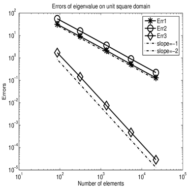
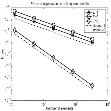
Figure 1. The errors for the eigenvalue approximations on unit square by ECR (left) and $EQ_{1}^{\rm rot}$ (right), where ${\rm Err1}=\sum_{j=1}^{6}(\lambda_{j}-\lambda_{j,h})$, ${\rm Err2}=\sum_{j=1}^{6}(\widehat{\lambda}_{j,h}-\lambda_{j})$ and ${\rm Err3}=\sum_{j=1}^{6}(\widetilde{\lambda}_{j,h}-\lambda_{j})$

6.2. Eigenvalue problem on the $L$ shape domain

In this subsection, we solve the eigenvalue problem (2.1) on the $L$ shape domain $\Omega=(-1,1)\times(-1,1)\setminus(-1,0)\times(-1,0)$. The aim here is also to find the approximations of the first $6$ eigenvalues $\lambda_{1},\lambda_{2},\cdots,\lambda_{6}$.

First, ECR element is applied to solve the eigenvalue problem and then the linear finite element to do the postprocessing on the series of meshes which are produced by Delaunay scheme. The quadratic element is applied to implement Algorithm 5.1. Table 7 shows the eigenvalue approximations of the first $6$ eigenvalues and the approximations by postprocessing method with linear element is presented in Table 8. Table 9 shows the numerical results of the postprocessing Algorithm 5.1 with quadratic element. From Table 7, we can find the numerical approximations of ECR element are lower bounds of the exact eigenvalues. Tables 8 and 9 show the upper bounds of the numerical approximations by the postprocessing method using linear and quadratic elements.

Table 7. ECR element for eigenvalue problem on $L$ shape domain

$h$	$\lambda_{1,h}$	$\lambda_{2,h}$	$\lambda_{3,h}$	$\lambda_{4,h}$	$\lambda_{5,h}$	$\lambda_{6,h}$
$0.2$	8.9126839	14.379736	18.200634	26.360803	27.160361	34.333785
$0.1$	9.3655553	14.954062	19.323660	28.615430	30.449112	39.363462
$0.05$	9.5439611	15.133230	19.625778	29.266600	31.451422	40.860929
$0.025$	9.6066551	15.181407	19.711040	29.459256	31.775515	41.305926
$0.0125$	9.6277308	15.193312	19.732422	29.506604	31.869752	41.426233
Trend	$\nearrow$	$\nearrow$	$\nearrow$	$\nearrow$	$\nearrow$	$\nearrow$

Table 8. Linear element for postprocessing method on $L$ shape domain

$h$	$\lambda_{1,h}$	$\lambda_{2,h}$	$\lambda_{3,h}$	$\lambda_{4,h}$	$\lambda_{5,h}$	$\lambda_{6,h}$
$0.2$	10.578106	16.642707	22.460586	36.034300	39.441562	52.785280
$0.1$	9.9724152	15.610430	20.469954	31.132236	34.109328	44.593560
$0.05$	9.7438532	15.309456	19.934653	29.958076	32.522745	42.389559
$0.025$	9.6728756	15.224811	19.786815	29.627051	32.086619	41.719036
$0.0125$	9.6521963	15.203927	19.750613	29.546869	31.965675	41.541732
Trend	$\searrow$	$\searrow$	$\searrow$	$\searrow$	$\searrow$	$\searrow$

Table 9. Quadratic element for postprocessing method on $L$ shape domain

$h$	$\lambda_{1,h}$	$\lambda_{2,h}$	$\lambda_{3,h}$	$\lambda_{4,h}$	$\lambda_{5,h}$	$\lambda_{6,h}$
$0.2$	9.7067976	15.233894	19.813091	29.809049	32.402601	42.472832
$0.1$	9.6691745	15.201608	19.744920	29.541711	32.011248	41.586610
$0.05$	9.6496097	15.197646	19.739617	29.522960	31.939132	41.497609
$0.025$	9.6432648	15.197293	19.739232	29.521572	31.921467	41.481392
$0.0125$	9.6414840	15.197258	19.739210	29.521488	31.916952	41.477779
Trend	$\searrow$	$\searrow$	$\searrow$	$\searrow$	$\searrow$	$\searrow$

Then, $EQ_{1}^{\rm rot}$ element is applied to solve the eigenvalue problem and then the bilinear finite element to do the postprocessing on the series of uniform rectangle meshes. Biquadratic element is employed to implement Algorithm 5.1. Table 10 shows the eigenvalue approximations of the first $6$ eigenvalues and the approximations by postprocessing method with bilinear element is presented in Table 11. Table 12 shows the numerical results of the postprocessing Algorithm 5.1 with biquadratic element. From Table 10, we can find the numerical approximations of $EQ_{1}^{\rm rot}$ element are lower bounds of the exact eigenvalues. Tables 11 and 12 show the upper bounds of the numerical approximations by the postprocessing method using bilinear and biquadratic elements.

Table 10. $EQ_{1}^{\rm rot}$ element for eigenvalue problem on $L$ shape domain

$h$	$\lambda_{1,h}$	$\lambda_{2,h}$	$\lambda_{3,h}$	$\lambda_{4,h}$	$\lambda_{5,h}$	$\lambda_{6,h}$
$1/4\times 1/4$	9.2784846	15.049120	19.477978	28.869068	30.381898	39.579205
$1/8\times 1/8$	9.5063501	15.154836	19.675337	29.348136	31.415853	40.855247
$1/16\times 1/16$	9.5896364	15.185968	19.723326	29.477224	31.747401	41.282853
$1/32\times 1/32$	9.6205870	15.194336	19.735243	29.510335	31.855244	41.413996
$1/64\times 1/64$	9.6323169	15.196509	19.738218	29.518686	31.891900	41.454533
Trend	$\nearrow$	$\nearrow$	$\nearrow$	$\nearrow$	$\nearrow$	$\nearrow$

Table 11. Bilinear element for postprocessing method on $L$ shape domain

$h$	$\lambda_{1,h}$	$\lambda_{2,h}$	$\lambda_{3,h}$	$\lambda_{4,h}$	$\lambda_{5,h}$	$\lambda_{6,h}$
$1/4\times 1/4$	10.164089	15.980053	20.773284	32.476652	35.807091	48.127411
$1/8\times 1/8$	9.7907347	15.392383	19.994161	30.245451	32.945969	43.311982
$1/16\times 1/16$	9.6867567	15.246072	19.802707	29.701314	32.192812	41.959311
$1/32\times 1/32$	9.6552886	15.209476	19.755068	29.566371	31.992010	41.603765
$1/64\times 1/64$	9.6451377	15.200312	19.743173	29.532700	31.936225	41.509772
Trend	$\searrow$	$\searrow$	$\searrow$	$\searrow$	$\searrow$	$\searrow$

Table 12. Biquadratic element for postprocessing method on $L$ shape domain

$h$	$\lambda_{1,h}$	$\lambda_{2,h}$	$\lambda_{3,h}$	$\lambda_{4,h}$	$\lambda_{5,h}$	$\lambda_{6,h}$
$1/4\times 1/4$	9.6733499	15.208409	19.749420	29.581107	32.072149	41.784684
$1/8\times 1/8$	9.6525125	15.198129	19.739857	29.525433	31.949976	41.516052
$1/16\times 1/16$	9.6447652	15.197334	19.739249	29.521742	31.925488	41.485165
$1/32\times 1/32$	9.6417221	15.197261	19.739211	29.521499	31.917575	41.478309
$1/64\times 1/64$	9.6405166	15.197253	19.739209	29.521483	31.914580	41.475981
Trend	$\searrow$	$\searrow$	$\searrow$	$\searrow$	$\searrow$	$\searrow$

Figure 2 shows the errors of the eigenvalue approximations by ECR and $EQ_{1}^{\rm rot}$ elements, postprocessing methods with lowest order (linear and bilinear) and higher order (quadratic and biquadratic) elements on the $L$ shape domain. Since we don’t know the exact eigenvalues on the $L$ shape domain, we can only give the errors of $\widehat{\lambda}_{j,h}-\lambda_{j,h}$ and $\widetilde{\lambda}_{j,h}-\lambda_{j,h}\ (j=1,2,3,4,5,6)$. Since the eigenfunctions here are singular, the convergence order by postprocessing with higher order element can not be improved which is shown in Figure 2.

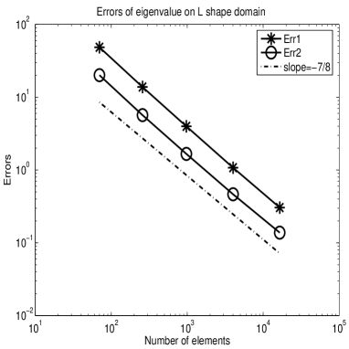
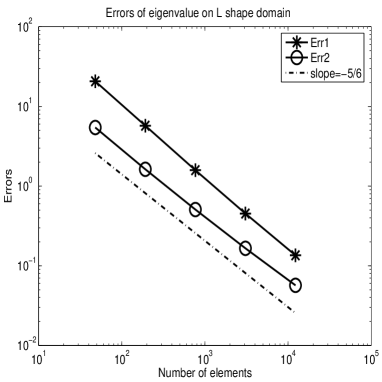
Figure 2. The errors for the eigenvalue approximations on $L$ shape domain by ECR (left) and $EQ_{1}^{\rm rot}$ (right), where ${\rm Err1}=\sum_{j=1}^{6}(\widehat{\lambda}_{j,h}-\lambda_{j,h})$ and ${\rm Err2}=\sum_{j=1}^{6}(\widetilde{\lambda}_{j,h}-\lambda_{j,h})$

7. Concluding remarks

In this paper, we analyzed the lower bound approximation of eigenvalue problem by nonconforming elements (ECR and $EQ_{1}^{\rm rot}$) and also two postprocessing methods to obtain the upper bound of the eigenvalues. Especially, based on the lower bound approximations, a new postprocessing method which can produce not only higher order convergence but also upper bound approximation of the eigenvalues is proposed. This improves the efficiency of solving eigenvalue problems and obtain the accurate a posteriori error estimates by the lower and upper bounds of eigenvalues.

We should point out that all the methods and results here can be easily extended to the three dimension case. We listed some related space and results. The corresponding $ECR$ element in $\mathcal{R}^{3}$ is defined as

$$V_{h}^{NC}:= \Big{\{}v\in L^{2}({\it\Omega}):v|_{K}\in{\rm span}\{1,x,y,z,x^{2}+y^{2}+z^{2}\},\int_{\ell}v|_{K_{1}}{\rm d}s=\int_{\ell}v|_{K_{2}}{\rm d}s,$$

(7.1) $$\hskip 28.45274pt\text{ when }K_{1}\cap K_{2}=\ell,\ \text{and }\int_{\ell}v|_{K}{\rm d}s=0,\text{ if }K\cap\partial{\it\Omega}=\ell\Big{\}},$$

where $K,K_{1},K_{2}\in\mathcal{T}_{h}$.

The corresponding $EQ_{1}^{\rm rot}$ element in $\mathcal{R}^{3}$ is defined as

$$V_{h}^{NC}:= \Big{\{}v\in L^{2}(\Omega):v|_{K}\in{\rm span}\{1,x,y,z,x^{2},y^{2},z^{2}\},\int_{\ell}v|_{K_{1}}ds=\int_{\ell}v|_{K_{2}}ds,$$

(7.2) $$\hskip 28.45274pt\text{if }K_{1}\cap K_{2}=\ell,\ \text{ and }\int_{\ell}v|_{K}ds=0,\text{ if}K\cap\partial\Omega=\ell\Big{\}},$$

where $K,K_{1},K_{2}\in\mathcal{T}_{h}$.

These two nonconforming elements can be used in the three dimensional case to get the lower bounds of eigenvalues and the corresponding postprocessing methods can also be constructed to obtain upper bounds of the eigenvalues.

References

- [1] M. Armentano and R. Duŕan, Asymptotic lower bounds for eigenvalues by nonconforming finite element methods, ETNA 17(2004), 93-101.
- [2] I. Babuška and J. Osborn, Finite element Galerkin approximation of the eigenvalues and eigenvectors of selfadjoint problem, Math. Comp., 52(1989), 275-297.
- [3] I. Babuška and J. Osborn, Eigenvalue Problems, in Handbook of Numerical Analysis, V. II: Finite Element Methods (Part I), Edited by P. G. Ciarlet and J. L. Lions, 1991, Elsevier.
- [4] P. Ciarlet, The Finite Element Method for Elliptic Problems, North-Holland, 1978.
- [5] F. Chatelin, Spectral Approzimations of Linear Operators, Academic Press, New York, 1983.
- [6] K. Feng, A difference scheme based on variational principle, Appl. Math and Comp. Math, 2(1965), 238-262.
- [7] J. Hu, Y. Huang and H. Shen, The lower approximation of eigenvalue by lumped mass finite element methods, J. Comput. Math., 22(2004), 545-556.
- [8] J. Hu, Y. Huang and Q. Lin, The analysis of the lower approximation of eigenvalues by nonconforming elements, to appear, 2010.
- [9] Y. Li, Lower approximation of eigenvalue by the nonconforming finite element method, Math. Numer. Sin., 30(2)(2008), 195-200.
- [10] Q. Lin, H. Huang and Z. Li, New expansions of numerical eigenvalues for by nonconforming elements, Math. Comput., 77(2008), 2061-2084.
- [11] Q. Lin and J. Lin, Finite Element Methods: Accuracy and Improvements, Science Press, Beijing, 2006.
- [12] Q. Lin, L. Tobiska and A. Zhou, On the superconvergence of nonconforming low order finite elements applied to the Poisson equation, IMA. J. Numer. Anal., 25(2005), 160-181.
- [13] Q. Lin, H. Xie, F. Luo, Y. Li and Y. Yang, Stokes eigenvalue approximation from below with nonconforming mixed finite element methods, Math. in Practice and theory, 19(2010), 157-168.
- [14] Q. Lin, H. Xie, and J. Xu, Lower bounds of the discretization for piecewise polynomials, http://arxiv.org/abs/1106.4395, 2011.
- [15] H. Liu and L. Liu, Expansion and extrapolation of the eigenvalue on element, Journal of Hebei University, 23(2005), 11-15.
- [16] H. Liu and N. Yan, Four finite element solutions and comparisions of problem for the Poisson equation eigenvalue, J. Numer. Method & Comput Appl, 2(2005), 81-91.
- [17] R. Rannacher, Nonconforming finite element methods for eigenvalue problems in linear plate theory, Numer Math 33, 23-42, 1979
- [18] G. Stang, G. Fix, An Analysis of the Finite Element Method, Englewood Cliffs, NJ: Prentice-Hall, 1973.
- [19] J. Xu and A. Zhou, A two-grid discretization scheme for eigenvalue problems, Math. Comput., 70(233)(2001), 17-25.
- [20] Y. Yang, Finite Element Methods Analysis to Eigenvalue Problem, Guizhou People Press, China, 2004.
- [21] Y. Yang, Z. Zhang and F. Lin, Eigenvalue approximation from below using nonforming finite elements, Sci. China Math., 53(1)(2010), 137-150.