Winning games for bounded geodesics in moduli spaces of quadratic differentials

Abstract.

We prove that the set of bounded geodesics in Teichmüller space are a winning set for Schmidt’s game. This is a notion of largeness in a metric space that can apply to measure $0$ and meager sets. We prove analogous closely related results on any Riemann surface, in any stratum of quadratic differentials, on any Teichmüller disc and for intervals exchanges with any fixed irreducible permutation.

1. Introduction

In the 1966 paper [15] W. Schmidt introduced a game, now called a Schmidt game, to be played by two players in $\mathbb{R}^{n}$. He showed that winning sets for his game are large in the sense that they have full Hausdorff dimension, and that the set of badly approximable vectors in $\mathbb{R}^{n}$, which were known to have measure zero, is a winning set for this game. Schmidt’s game and a modified version of it were used in [3] and [9] to establish that the set of bounded trajectories of nonquasiunipotent flow on a finite volume homogeneous space has full Hausdorff dimension, a result first established in [7] using different methods. The dynamical significance of badly approximable vectors is well-understood: in terms of the flow on the moduli space of $(n+1)$-dimensional tori $\operatorname{SL}(n+1,\mathbb{R})/\operatorname{SL}(n,\mathbb{Z})$ induced by the left action of the one-parameter subgroup $g_{t}=\operatorname{diag}(e^{t},\dots,e^{t},e^{-nt})$, a vector $\mathbf{x}\in\mathbb{R}^{n}$ is badly approximable if and only if it determines a bounded trajectory via $g_{t}U(\mathbf{x})\operatorname{SL}(n+1,\mathbb{Z})$ where $U(\mathbf{x})$ is the unipotent matrix whose $(i,j)$-entry is $1$ if $i=j$, $-x_{i}$ if $i\leq n$ and $j=n+1$, and $0$ otherwise.

This paper is concerned with higher genus analogues of the same circle of ideas. Let $\mathcal{PMF}$ be Thurston’s sphere of projective measured foliations on a closed surface of genus $g>1$. Let $D\subset\mathcal{PMF}$ consist of those foliations $F$ such that for some (hence all) quadratic differentials $q$ whose vertical foliation is $F$, the Teichmüller geodesic defined by $q$ stays in a compact set in $\mathcal{M}_{g}$, the moduli space of genus $g$. Following [11], we use the terminology Diophantine to describe the foliations that lie in the set $D$. It was shown in [11] that a foliation $F$ is Diophantine if and only if

$$\inf_{\beta}|\beta|i(F,\beta)>0.$$

Here, the infimum is over all homotopy classes of simple closed curves $\beta$, $i(F,\beta)$ is the standard intersection number, and for $|\beta|$ one can take it to be the length of the geodesic in the homotopy class with respect to some fixed hyperbolic structure on the surface. The notion of Diophantine does not depend on which hyperbolic metric is chosen. Alternatively, we may fix a triangulation of the surface and take the number $|\beta|$ to be the minimum number of edges traversed by any curve in the homotopy class. In the moduli space of genus one, a.k.a. the modular surface, Teichmüller geodesic rays are represented by arcs of circles or vertical lines in the upper half plane with endpoint in $\mathbb{R}\cup\{\infty\}$. The notion of Diophantine extends the property of a geodesic ray that its endpoint is a badly approximable real number.

In [10] McMullen introduced two variants of the Schmidt game, giving rise to the notions of strong winning and absolute winning sets. (We recall their definitions in the next section.) It is not hard to show that absolute winning implies strong winning while strong winning implies Schmidt winning, i.e. winning in the original sense of Schmidt. In particular, they also have full Hausdorff dimension. McMullen raises the question in [10] as to whether the set of Diophantine foliations $D\subset\mathcal{PMF}$ is a strong winning set. In this paper, we give an affirmative answer to this question.

Theorem 1.1.

The set $D\subset\mathcal{PMF}$ of Diophantine foliations is a strong winning set, hence a winning set for the Schmidt game. However, it is not absolute winning.

We remark that the Schmidt game requires a metric on the space, but the notion of winning is invariant under bi-Lipschitz equivalence. In the case of $\mathcal{PMF}$ there are various bi-Lipschitz equivalent ways of defining a metric. The most familiar is to use train track coordinates. (See [14] for a discussion of train tracks). A fixed train track defines a local metric by pull-back of the Euclidean metric. A finite collection of train tracks can be used to parametrize all of $\mathcal{PMF}$. One can then defined a path metric on $\mathcal{PMF}$ via a finite number of locally defined metrics.

The next theorem concerns quadratic differentials (see Section 3 for the definition of quadratic differentials) that determine bounded geodesics in a stratum.

Theorem 1.2.

Let $Q^{1}(k_{1},\ldots,k_{n},\pm)$ be any stratum of unit norm quadratic differentials. Let $U$ be an open set with compact closure $\bar{U}\subset Q^{1}(k_{1},\ldots,k_{n},\pm)$ with a metric given by the pull-back of the Euclidean metric under a local coordinate system given by the holonomy coordinates of saddle connections. Then there exists an $\alpha>0$ depending on the smallest systole in $U$ such that the subset $E_{Q}\subset\bar{U}$ consisting of those quadratic differentials $q$ such that the Teichmüller geodesic defined by $q$ stays in a compact set in the stratum is an $\alpha$-strong winning, hence winning for the Schmidt game. It is not absolute winning.

Again we remark that the metric is not canonical as it depends on a choice of coordinates. However different choices give bi-Lipschitz equivalent metrics and the notion of winning is well-defined. We remark that bounded has a slightly more restrictive meaning here than in the case of $\mathcal{PMF}$ in that in this case no saddle connection gets short along the geodesic, while in the case of $\mathcal{PMF}$ the condition is slightly weaker in that no simple closed curve gets short. The difference in definitions is accounted for by the fact that points in $\mathcal{PMF}$ are only defined up to equivalence by Whitehead moves ([4]) which collapse leaves of a foliation joining singularities to a higher order singularity. Thus quadratic differentials whose vertical foliations determine the same point in $\mathcal{PMF}$ may lie in different strata.

Theorem 1.3.

Fix a closed Riemann surface $X$ of genus $g>1$ and let $Q^{1}(X)$ denote the space of unit norm holomorphic quadratic differentials on $X$. Then the set of $q\in Q^{1}(X)$ that determine a Teichmüller geodesic that stays in a compact set of the stratum is strong winning, hence Schmidt winning. It is not absolute winning.

Here the distance is defined by the norm; namely $d(q_{1},q_{2})=\|q_{1}-q_{2}\|$.

Theorem 1.4.

Let $\Lambda$ denote the simplex of interval exchange transformations $(T,\lambda,\pi)$ on $n$ intervals with a fixed irreducible permutation $\pi$ defined on the unit interval $[0,1)$. We give $\Lambda$ the Euclidean metric. Let $E_{B}$ consist of the bounded $(T,\lambda,\pi)$. This means that $\inf_{n}n|T^{n}(p_{1})-p_{2}|>0$, where $p_{1},p_{2}$ are discontinuities of $T$. Then $E_{B}$ is strong winning hence Schmidt winning. It is not absolute winning.

Because winning has nice intersection properties we obtain the following result that there are many interval exchange transformations which are bounded and any reordering of the lengths is also bounded.

Corollary 1.1.

Let $E_{B}$ be as in Theorem 1.4. Then the set

$$\{\lambda\in\Lambda:(\lambda_{i_{1}},...\lambda_{i_{n}})\in E_{B}\text{ for all }\{i_{1},...,i_{n}\}=\{1,...,n\}\}$$

is nonempty. In fact, it has full Hausdorff dimension.

The main theorem we prove from which the other theorems will follow is a one-dimensional version.

Theorem 1.5.

Let $q$ be a holomorphic quadratic differential on a closed Riemann surface of genus $g>1$. Then the set $E$ of directions $\theta$ in the circle $S^{1}$ with the Euclidean metric such that the Teichmüller geodesic defined by $e^{i\theta}q$ stays in a compact set of the corresponding stratum in the moduli space of quadratic differentials is an absolute winning set; hence strong winning.

In Theorem 1.5 we call the directions in $E$ bounded directions. Here is an equivalent formulation of Theorem 1.5 (Proposition LABEL:equiv_cond establishes the equivalence).

Theorem 1.6.

Let

$$S=\{(\theta,L):\theta\text{ is the direction of a saddle connection of $q$ of length }L\}.$$

Then the set $E$ of bounded directions $\psi$ in the circle is the same as

$$\{\psi:\underset{(\theta,L)\in S}{\inf}L^{2}|\theta-\psi|>0\}$$

and this is an absolute winning set.

As an immediate corollary we get the following result which was first proved by Kleinbock and Weiss [8] using quantitative non-divergence of horocycles [13].

Corollary 1.2.

The set of directions such that the Teichmüller geodesic stays in a compact subset of the stratum has Hausdorff dimension $1$.

It is well-known that a billiard in a polygon $\Delta$ whose vertex angles are rational multiples of $\pi$ gives rise to a translation surface by an unfolding process. We have the following corollary to Theorem 1.6.

Corollary 1.3.

Let $\Delta$ be a rational polygon. The set $E$ of directions $\theta$ for the billiard flow in $\Delta$ with the property that there is an $\epsilon=\epsilon(\theta)>0$, so that for all $L>0$, the billiard path in direction $\theta$ of length smaller than $L$ starting at any vertex, stays outside an $\frac{\epsilon}{L}$ neighborhood of all vertices of $\Delta$, is an absolute winning set.

Since for any $0<\alpha<2\pi$ and $n\in\mathbb{Z}$, the set $E+n\alpha$ (mod $2\pi$) is an isometric image of $E$, it is also Schmidt winning with the same winning constant for each $n$. Therefore, the infinite intersection $\cap_{n\in\mathbb{Z}}(E+n\alpha)$ is Schmidt winning, and thus has Hausdorff dimension $1$. This gives the following corollary.

Corollary 1.4.

For any $\alpha$ there is a Hausdorff dimension $1$ set of angles $\theta$ such that for any $n$, there is $\epsilon_{n}>0$ such that a billiard path at angle $\theta+n\alpha(mod(2\pi))$ and length at most $L$ from a vertex does not enter a neighborhood of radius $\frac{\epsilon_{n}}{L}$ of any vertex.

Another corollary uses the absolute winning property but does not follow just from Schmidt winning. Let $E$ be the set from Corollary 1.3.

Corollary 1.5.

The set $E^{\prime}=\{\theta:\forall n\in\mathbb{Z}_{>0},n\theta\in E\}$ has Hausdorff dimension $1$.

The core theorems that we prove are Theorem 1.5 for the set of bounded directions in the disc and Theorem 1.2 for winning in the stratum. The former is a model for the latter although the former proves absolute winning and the latter strong winning. The fairly general Theorem 2.1 will reduce Theorem 1.1 and Theorem 1.4 to Theorem 1.2. Theorem 1.3 reduces to Theorem 1.1.

1.1. Acknowledgments

The authors would like to thank Dmitry Kleinbock and Barak Weiss for telling the first author about this delightful problem and helpful conversations and to thank Curtis McMullen for his conversations with the third author. The authors would also like to thank the referee for numerous helpful suggestions.

2. Strong and absolute winning sets

2.1. Schmidt games

We describe the Schmidt game in $\mathbb{R}^{n}$. Suppose we are given a set $E\subset\mathbb{R}^{n}$. Suppose two players Bob and Alice take turns choosing a sequence of closed Euclidean balls

$$B_{1}\supset A_{1}\supset B_{2}\supset A_{2}\supset B_{3}\ldots$$

(Bob choosing the $B_{i}$ and Alice the $A_{i}$) whose diameters satisfy, for fixed $0<\alpha,\beta<1$,

(1) $$|A_{i}|=\alpha|B_{i}|\quad\text{and}\quad|B_{i+1}|=\beta|A_{i}|.$$

Following Schmidt

Definition 2.1.

We say $E$ is an $(\alpha,\beta)$-winning set if Alice has a strategy so that no matter what Bob does, $\cap_{i=1}^{\infty}B_{i}\in E$. It is $\alpha$-winning if it is $(\alpha,\beta)$-winning for all $0<\beta<1$. $E$ is a winning set for Schmidt game if it is $\alpha$-winning for some $\alpha>0$.

Their main properties, proved by Schmidt in [15], are:

• they have full Hausdorff dimension,

• they are preserved by bi-Lipschitz mappings (the constant $\alpha$ can change),

• a countable intersection of $\alpha$-winning sets is $\alpha$-winning.

McMullen [10] suggested two variants of the Schmidt game as follows. The first variant replaces (1) with

(2) $$|A_{i}|\geq\alpha|B_{i}|\quad\text{and}\quad|B_{i+1}|\geq\beta|A_{i}|.$$

The notions of $(\alpha,\beta)$-strong and $\alpha$-strong winning sets are similarly defined. (Bob wins if $\cap_{i=1}^{\infty}B_{i}\cap E=\emptyset$; otherwise, Alice wins). A strong winning set refers to a set that is $\alpha$-strong winning for some $\alpha>0$.

In the second variant, the sequence of balls $B_{i}$, $A_{i}$ must be chosen so that

$$B_{1}\supset B_{1}\setminus A_{1}\supset B_{2}\supset B_{2}\setminus A_{2}\supset B_{3}\supset\dots$$

and for some fixed $0<\beta<1/3$,

$$|A_{i}|\leq\beta|B_{i}|\quad\text{and}\quad|B_{i+1}|\geq\beta|B_{i}|.$$

We say $E$ is $\beta$-absolute winning if Alice has a strategy that forces $\cap_{i=1}^{\infty}B_{i}\cap E=\emptyset$ regardless of how Bob responds. An absolute winning set is one that is $\beta$-absolute winning for all $0<\beta<1/3$. (Remark: The condition $\beta<1/3$ ensures Bob always has moves available to him no matter how Alice plays her moves.) It is also clear that if a set is absolute winning for some $\beta_{0}$ then it is absolute winning for $\beta>\beta_{0}$.

As noted in the introduction, absolute winning implies strong winning, which in turn implies winning in the sense of Schmidt. In particular, both types of sets have full Hausdorff dimension. These notions provide two new classes of sets that also have the countable intersection property and are not only bi-Lipschitz invariant, but preserved by the much larger class of quasi-symmetric homeomorphisms. (See [10].) As McMullen notes, most sets known to be winning in the sense of Schmidt are in fact strong winning, as is the case with the set of badly approximable vectors in $\mathbb{R}^{n}$. Since any subset of $\mathbb{R}^{n}$ that contains a line segment in its complement cannot be absolute winning (because Bob can always choose $B_{j}$ centered at a point on this line segment), the set of badly approximable vectors in $\mathbb{R}^{n}$ ($n\geq 2$) provides a natural example of a strong winning set that is not absolutely winning. However, it is far from obvious that there are winning sets in the sense of Schmidt that are not strong winning ([10]).

2.2. Projections and the simultaneous blocking game

Theorem 1.1 and Theorem 1.4 will follow from Theorem 1.2 by use of the following fairly general statement.

Definition 2.2.

A surjective map $f:X\to Y$ between metric spaces is a quasi-symmetry if there exists $0<c<1$ such that for all $(x,r)\in X\times\mathbb{R}_{+}$,

$$B_{Y}(f(x),cr)\subset f(B_{X}(x,r))\subset B_{Y}(f(x),r/c).$$

Theorem 2.1.

Suppose $f:X\to Y$ is a surjective quasi-symmetry between complete metric spaces and $E\subset X$ is $\alpha$-strong winning. Then $f(E)$ is $c^{2}\alpha$-strong winning. (Here winning means that once Bob chooses an initial ball in $Y$ then Alice has a strategy to force the intersection point to lie in $f(E)$).

We remark that linear projection maps from $\mathbb{R}^{n}$ onto subspaces obviously satisfy the hypotheses and these are what will occur in the proofs of Theorem 1.1 and Theorem 1.4, but we wish to prove a more general theorem.

Proof.

First we claim that if $s<r,r_{0}^{\prime},x_{0}^{\prime}\in X,z\in Y$, and $y^{\prime}\in B_{X}(x_{0}^{\prime},r_{0}^{\prime})$ are such that $B_{Y}(z,s)\subset B_{Y}(f(y^{\prime}),cr)$ then there exists $z^{\prime}\in f^{-1}(z)$ such that $B_{X}(z^{\prime},s)\subset B_{X}(y^{\prime},r)$. We prove the claim.

Since $B_{Y}(z,s)\subset B_{Y}(f(y^{\prime}),cr)$ we have $B_{Y}(z,cs)\subset B_{Y}(f(y^{\prime}),cr)$ which in turn implies that $z\in B_{Y}(f(y^{\prime}),c(r-s))$. It follows from the hypotheses of the Theorem that there is a $z^{\prime}\in B_{X}(y^{\prime},r-s)$ such that $f(z^{\prime})=z$. The triangle inequality now implies that $B_{X}(z^{\prime},s)\subset B_{X}(y^{\prime},r)$, proving the claim.

Now we show that $f(E)$ is $(c^{2}\alpha,\beta)$-strong winning in $Y$ by winning an auxiliary $(\alpha,c^{2}\beta)$-strong winning game in $X$. We describe the inductive strategy. We are given $B_{X}(x_{k},r)$ and $B_{Y}(f(x_{k}),cr)$ where $B_{X}(x_{k},r)$ is part of Alice’s $(\alpha,c^{2}\beta)$-strong winning strategy in $X$ and $B_{Y}(f(x_{k}),cr)$ is Alice’s move in the $(c^{2}\alpha,\beta)$-game in $Y$. Bob chooses $B_{Y}(z,s)\subset B_{Y}(f(x_{k}),cr)$ and $s\geq\beta cr$.

By the claim there exists $z^{\prime}\in f^{-1}(z)$ such that

$$B_{X}(z^{\prime},cs)\subset B_{X}(x_{k},r)\text{ with }cs\geq c^{2}\beta r.$$

So $B_{X}(z^{\prime},cs)$ is a legal move in the $(\alpha,c^{2}\beta)$-strong winning game (in $X$) given Alice’s move $B_{X}(x_{k},r)$. So Alice has a response

$$B_{X}(x_{k+1},t)\subset B_{X}(z^{\prime},cs)\text{ and }t\geq\alpha cs$$

as part of her $(\alpha,c^{2}\beta)$-strong winning strategy in $X$, which we assumed existed.

Now

$$B_{Y}(f(x_{k+1}),ct)\subset f(B_{X}(x_{k+1},t))\subset f(B_{X}(z^{\prime},cs))\subset B_{Y}(z,s)\text{ and }ct\geq c^{2}\alpha s.$$

So it is a legal move for the $(c^{2}\alpha,\beta)$-strong winning game given Bob’s move $B_{Y}(z,s).$

Because the auxiliary game is a legal $(\alpha,c^{2}\beta)$-game we have $\cap_{k=1}^{\infty}B_{X}(x_{k},r_{k})\in E$. Thus

$$\cap_{k=1}^{\infty}B_{Y}(f(x_{k}),cr)\subset\cap_{k=1}^{\infty}f(B_{X}(x_{k},r))\in f(E).$$

So $f(E)$ is $(c^{2}\alpha,\beta)$-strong winning. ∎

To prove Theorem 1.5, (played on the circle $S^{1}$) it will be convenient to consider a variation on the absolute winning game where Alice is permitted to simultaneously block $M$ intervals of radii $\leq\beta|I_{j}|$. (The condition $(2M+1)\beta<1$ ensures that Bob will always have available moves.)

Lemma 2.1.

Suppose $E$ is a winning set for the modified game where Alice is permitted to simultaneously block $M$ intervals of length at most $\beta^{M}$ times the length of Bob’s interval. Then $E$ is an absolute winning set with the parameter $\beta$.

Proof.

Let $I_{j},j\geq 1$ denote the intervals that Bob plays in the (original) absolute game. Alice will consider the subsequence $I_{1+rM},r\geq 0$ as Bob’s moves in the modified game. Given $j=1\mod M$ Alice considers the intervals $J_{1},\dots,J_{M}$ she would have played in the modified game in response to Bob’s choice of $I_{j}$. The strategy for her next $M$ moves of the original game is to pick

$$U_{j}=J_{1},\quad U_{j+1}=J_{2}\cap I_{j+1},\quad U_{j+2}=J_{3}\cap I_{j+2},\quad\dots\quad U_{j+M-1}=J_{M}\cap I_{j+M-1}.$$

Observe that for $i=1,\dots,k-1,$

$$|U_{j+k-1}|\leq|J_{k}|\leq\beta^{M}|I_{j}|\leq\beta^{M-i}|I_{j+i}|\leq\beta|I_{j+k-1}|$$

so Alice’s choice of $U_{j+k-1}$ in response to $I_{j+k-1}$ is valid. Note that $|I_{j+M}|\geq\beta^{M}|I_{j}|$ and that $I_{j+M}$ is disjoint from $J_{k}$ because $I_{j+M}\subset I_{j+k}$ and Bob is required to choose $I_{j+k}$ disjoint from $J_{k}$ inside $I_{j+k-1}$. Thus, $I_{j+M}$ is a valid move for Bob in the modified game so that Alice can continue her next $M$ moves by repeating the strategy just described.

Since the intervals $I_{j}$ are nested, we have

$$\bigcap_{j=1}^{\infty}I_{j}=\bigcap_{r=1}^{\infty}I_{1+rM},$$

which has nontrivial intersection with $E$, by hypothesis. ∎

We remark that there is an obvious partial converse: if Alice can win the absolute game then she can also win the modified game with the same parameter. Indeed, she simply picks all her $M$ intervals to be the same as the interval she would have chosen in the original, absolute game.

2.3. Case of badly approximable numbers

Recall that a real number $\theta$ is badly approximable if there exists $c>0$ such that for all rationals $p/q\in\mathbb{Q}$

$$\left|\theta-\frac{p}{q}\right|>\frac{c}{q^{2}}.$$

The fact that the set of badly approximable numbers is absolute winning is a special case of Theorem 1.3 of [10]. We give a proof of this result because it serves as a motivation for the proof of Theorem 1.5.

Theorem 2.2.

The set of badly approximable real numbers is absolute winning.

Proof.

Fix $\varepsilon>0$. Given an interval $B_{j}$ chosen by Bob, let $I_{j}$ be an $\varepsilon|B_{j}|$-neighborhood of $B_{j}$ and let $p_{j}/q_{j}$ be the rational of smallest denominator (in lowest terms) in the interval $I_{j}$. Alice’s strategy is to ”block $p_{j}/q_{j}$”; in other words, she picks

$$A_{j}=\left(\frac{p_{j}}{q_{j}}-\frac{\beta|B_{j}|}{2},\frac{p_{j}}{q_{j}}+\frac{\beta|B_{j}|}{2}\right).$$

We claim that there exists $c>0$ such that $|I_{j}|q_{j}^{2}>c$ for all $j\geq 1$. Indeed, if $q_{j+1}<\beta^{-1}q_{j}$ then

(3) $$|I_{j}|>\left|\frac{p_{j}}{q_{j}}-\frac{p_{j+1}}{q_{j+1}}\right|\geq\frac{1}{q_{j}q_{j+1}}>\frac{\beta}{q_{j}^{2}}$$

whereas if $q_{j+1}\geq\beta^{-1}q_{j}$ we have

$$|I_{j+1}|q_{j+1}^{2}\geq\beta|I_{j}|q_{j+1}^{2}\geq\beta^{-1}|I_{j}|q_{j}^{2}.$$

Now whenever the quantity $|I_{j}|q_{j}^{2}$ is less than $\beta$, the above inequality says it must increase by a factor of at least $\beta^{-1}$ at each step until it exceeds $\beta$, after which it may decrease by a factor of at most $\beta$ (since $|I_{j+1}|\geq\beta|I_{j}|$ and $q_{j+1}\geq q_{j}$) and then exceed $\beta$ again at the following step. Hence, $\liminf|I_{j}|q_{j}^{2}>\beta^{2}$ and the claim follows.

Given $x\in\cap B_{j}$ and $p/q\in\mathbb{Q}$, suppose first that $p/q\not\in I_{1}$. Then

$$\left|x-\frac{p}{q}\right|\geq\varepsilon|B_{1}|\geq\frac{\varepsilon|B_{1}|}{q^{2}}.$$

Thus assume $p/q\in I_{1}$. Since our strategy guarantees that $p/q\notin\cap I_{j}$, there is a (unique) index $j$ such that $p/q\in I_{j}\setminus I_{j+1}$ and $q_{j}\leq q$ (because $p/q\in I_{j}$) and since $p/q\not\in I_{j+1}$ we have

$$\left|x-\frac{p}{q}\right|\geq\varepsilon|B_{j+1}|\geq\beta\varepsilon|B_{j}|>\frac{c\beta\varepsilon|I_{j}|}{1+2\varepsilon}>\frac{c\beta\varepsilon}{(1+2\varepsilon)q_{j}^{2}}\geq\frac{c\beta\varepsilon}{(1+2\varepsilon)q^{2}}$$

proving $x$ is badly approximable. ∎

2.4. Sketch of the proofs of Theorem 1.5 and Theorem 1.2

In the game played with quadratic differentials on a higher genus surface, we have a similar criterion as for the torus, given by Proposition 1 that for a Teichmüller geodesic to lie in a compact set in the stratum, the direction is far from the direction of a saddle connection. This says that in order to show this set is winning we want to find a strategy giving us a point far from the direction of any saddle connection. Unlike the genus one case we have the major complication that directions of saddle connections in general need not be separated in the sense that the angle between them need not be at least a constant over the product of their lengths as it is in the case of tori. Equivalently, it may happen that on some flat surfaces there are many intersecting short saddle connections. This forces us to consider complexes of saddle connections that become simultaneously short under the geodesic flow. We call these complexes shrinkable.

An important tool is a process of combining a pair of shrinkable complexes of a certain level or complexity to build a shrinkable complex of higher level. This is given by Lemma 3.8 with the preliminary Lemma 3.6. These ideas are not really new; having appeared in several papers beginning with [6].

The main point in this paper and the strategy is given by Theorem 4.1. We show first that complexes of highest level are separated, as in the case of the torus, for otherwise we could combine them to build a complex of higher level that is shrinkable. This is impossible by definition of highest level. We develop a strategy for Alice where, as in the torus case, she blocks these highest level complexes. Then we consider complexes of one lower level that lie in the complement of the interval used to block highest level intervals and which are not too long in a certain sense depending on the stage of the game. We show that these are separated as well, for if not, we could combine them into a highest level complex of bounded size and these have supposedly been blocked at an earlier stage of the game. Thus there can be at most one such lower level complex (up to a certain combinatorial equivalence) and we block it. We continue this process inductively considering complexes of decreasing level one step at a time, ending by blocking single saddle connections. Then after a fixed number of steps we return to blocking highest level complexes and so forth. From this strategy, Theorem 1.5 will follow. For technical reasons, we need to block complexes by intervals whose length is comparable to the reciprocal of the product of their longest saddle connection and the longest saddle connection on their boundary.

In adapting the argument to the proof of Theorem 1.2, we need to consider complexes on distinct flat surfaces. In order to combine them so that Lemma 3.8 can be applied, we need to consider the problem of moving a complex on one surface to a nearby one. (See Theorem 5.1.) This operation is not canonical since unlike parallel transport, it does not respect the operation of concatenation along paths. However it does preserve inclusion of complexes (Proposition 2) and this is sufficient for our purposes. While the basic strategy is the same as that in the proof of Theorem 1.5, we caution the reader that unlike the ordinary and strong winning games, after Alice chooses $A_{j}$, the game ”continues” in $B_{j}\setminus A_{j}$ rather than inside $A_{j}$. In particular, we do not have an analog of the simultaneous blocking strategy Lemma 2.1.

3. Quadratic differentials, complexes, and geodesic flow

3.1. Quadratic differentials

A general reference here is [12]. Recall a holomorphic quadratic differential $q=\phi(z)dz^{2}$ on a Riemann surface $X$ of genus $g>1$ defines for each local holomorphic coordinate $z$, a holomorphic function $\phi_{z}(z)$ such that in overlapping coordinate neighborhoods $w=w(z)$ we have

$$\phi_{w}(w)\left(\frac{dw}{dz}\right)^{2}=\phi_{z}(z).$$

On a compact surface, $q$ has a finite set $\Sigma$ of zeroes. On the complement of $\Sigma$ there are natural local coordinates $z$ such that $\phi_{z}(z)\equiv 1$ and hence $q$ defines a flat surface. A zero of order $k$ defines a cone singularity of angle $(k+2)\pi$. Suppose $q$ has zeroes of orders $k_{1},\ldots,k_{p}$ with $\sum k_{i}=4g-4$. There is a moduli space or stratum $Q=Q(k_{1},\ldots,k_{p},\pm)$ of quadratic differentials all of which have zeroes of orders $k_{i}$. The $+$ sign occurs if $q$ is the square of an Abelian differential and the $-$ sign otherwise.

A quadratic differential $q$ defines an area form $|\phi(z)||dz^{2}|$ and a metric $|\phi|^{1/2}|dz|$. We assume that our quadratic differentials have area one. Recall a saddle connection is a geodesic in the metric joining a pair of zeroes which has no zeroes in its interior. By the systole of $q$ we mean the length of the shortest saddle connection.

A choice of a branch of $\phi^{1/2}(z)$ along a saddle connection $\beta$ and an orientation of $\beta$ determines a holonomy vector

$$hol(\beta)=\int_{\beta}\phi^{1/2}dz\in\mathbb{C}.$$

It is defined up to sign. Thinking of this as a vector in $\mathbb{R}^{2}$ gives us the horizontal and vertical components defined up to sign. We will denote by $h(\gamma)$ and $v(\gamma)$ the absolute value of these components. We will denote its length $|\gamma|$ as the maximum of $h(\gamma)$ and $v(\gamma)$. This slightly different definition will cause no difficulties in the sequel.

Given $\epsilon>0$, let $Q^{1}_{\epsilon}$ denote the compact set of unit area quadratic differentials in the stratum such that the shortest saddle connection has length at least $\epsilon$. The group $SL(2,\mathbb{R})$ acts on $Q^{1}$ and on saddle connections. (In the action we will suppress the underlying Riemann surface). Let

$$g_{t}=\left(\begin{array}[]{cc}e^{t}&0\\ 0&e^{-t}\end{array}\right)$$

denote the Teichmüller flow acting on $Q^{1}$ and

$$r_{\theta}=\left(\begin{array}[]{cc}\cos\theta&\sin\theta\\ -\sin\theta&\cos\theta\end{array}\right)$$

denote the rotation subgroup.

The Teichmüller flow acts by expanding the horizontal component of saddle connections by a factor of $e^{t}$ and contracting the vertical components by $e^{t}$. For $\sigma$ a saddle connection we will also use the notation $g_{t}r_{\theta}\sigma$ for the action on saddle connections. The action of $SL(2,\mathbb{R})$ is linear on holonomy of saddle connections.

Definition 3.1.

We say a direction $\theta$ is bounded if there exists $\epsilon$ such that $g_{t}r_{\theta}q\in Q^{1}_{\epsilon}$ for all $t\geq 0$.

3.2. Conditions for $\beta$-absolute winning

Definition 3.2.

Given a saddle connection $\gamma$ on $q$ we denote by $\theta_{\gamma}$ the angle such that $\gamma$ is vertical with respect to $r_{\theta_{\gamma}}q$.

We can think of the set of saddle connections as a subset of $S^{1}\times\mathbb{R}$ by associating to each $\gamma$ the pair $(\theta_{\gamma},|\gamma|)$. The following proposition gives the equivalence of Theorem 1.5 and Theorem 1.6 and will be the motivation for what follows.

Proposition 1.

Let

$$S=\{(\theta,L):\theta\text{ is the vertical direction of a saddle connection of length }L\}.$$

Then $\underset{(\theta,L)\in S}{\inf}L^{2}|\theta-\psi|>0$, if and only if $\psi$ determines a bounded direction.

Proof.

If $(\theta,L)\in S$, let $c=|\theta-\psi|$. We can assume $c\leq\frac{\pi}{4}$. Then the length of the saddle connection in $g_{t}r_{\psi}q$ coming from $(\theta,L)$ is $\max\{e^{t}\sin(c)L,e^{-t}L\cos(c)\}$ and minimized in $t$ when equality of the two terms holds; that is when $e^{-t}=\sqrt{\tan(c)}$. At this time the length is

$$L\sqrt{\sin(c)\cos(c)}=L\sqrt{\frac{\sin(2c)}{2}}\geq L\sqrt{\frac{c}{2}}.$$

So if $c>\frac{\delta}{L^{2}}$, for some $\delta>0$, then

$$\max\{e^{t}\sin(c)L,e^{-t}L\cos(c)\}>\sqrt{\frac{\delta}{2}}.$$

Conversely, if the minimum length $L\sqrt{\frac{\sin(2c)}{2}}$ is bounded below by some $\ell_{0}$ then the difference in angles $c$ satisfies

$$2c\geq\sin(2c)\geq\frac{2\ell_{0}^{2}}{L^{2}}.$$

∎

3.3. Complexes

In this section we fix a quadratic differential $q$. Let $\Gamma$ be a collection of saddle connections of $q$, any two of which are disjoint except possibly at a common zero. Let $K$ be the simplicial complex having $\Gamma$ as its set of $1$-simplices and whose $2$-simplices consist of all triangles that have all three edges in $\Gamma$. By a complex we mean any simplicial complex that arises in this manner. We shall also use the same term to mean the closed subset $K$ of the surface given by the union of all simplices; in this case, we call $\Gamma$ a triangulation of $K$. We shall often leave it to the context to determine which sense of the term is intended. For example, “a saddle connection in $K$” refers to an element of $\Gamma$, whereas “the interior of $K$” refers to the largest open subset contained in $K$, which may be empty. An edge $e$ is in the topological boundary $\partial K$ of $K$ if any neighborhood of an interior point of $e$ intersects the complement of $K$. We note that the boundary of a complex may fail to satisfy the requirement that a triangle with edges in the complex is also included in the complex, as happens when $K$ is simply a triangle.

We distinguish between internal saddle connections in $\partial K$, which lie on the boundary of a $2$-simplex in $K$ and external ones, which do not. Note that a triangulation $\Gamma$ of $K$ may contain both internal and external saddle connections. The remaining saddle connections are on the boundary of two $2$-simplices, and we refer to them as interior saddle connections, which, of course, depend on the choice of $\Gamma$. Each internal saddle connection comes with a transverse orientation, which is determined by the choice of an inward normal vector at any interior point of the segment. The interior of $K$ is determined by the data consisting of $\partial K$, the subdivision into internal and external saddle connections, together with the choice of transverse orientation for each internal saddle connection. Simplicial homeomorphisms respect these notions in the obvious sense, while simplicial maps generally do not.

Definition 3.3.

The level of a complex is the number of edges in any triangulation.

An easy Euler characteristic argument says that the level $M$ is well defined and is bounded by $6g-6+3n$, where $n$ is the number of zeroes.

We say two complexes are topologically equivalent if they determine the same closed subset of the surface. Otherwise, they are topologically distinct.

Lemma 3.1.

If $K_{1}$ and $K_{2}$ are topologically distinct complexes of the same level, then any triangulation of $K_{2}$ contains a saddle connection $\gamma\in K_{2}$ that intersects the exterior of $K_{1}$, i.e. $\gamma\not\subset K_{1}$.

Proof.

Arguing by contradiction, we suppose that the conclusion does not hold. Then there is a triangulation of $K_{2}$ such that every edge is contained in $K_{1}$. It would follow that $K_{2}\subset K_{1}$, and properly so, since they are topologically distinct. By repeatedly adding saddle connections $\sigma\subset K_{1}$ that are disjoint from those in $K_{2}$, we can extend the triangulation of $K_{2}$ to one of $K_{1}$ to obtain one where the number of edges is strictly greater than the level of $K_{1}$. This contradicts the fact that any two triangulations of a complex contains the same number of edges. ∎

A path in $\Gamma$ refers to a sequence of edges in $\Gamma$ such that the terminal endpoint of the previous edge coincides with the initial endpoint of the next edge. We may also think of it as a map of the unit interval into $X$. The combinatorial length of a path in $\Gamma$ refers to the number of edges in the sequence, including repetitions. For a homotopy class of paths with endpoints fixed at the zeroes of $q$ we define the combinatorial length to be the minimum combinatorial length of a path in $\Gamma$ in the homotopy class. We denote the combinatorial length of a saddle connection by $|\gamma|_{\Gamma}$.

To show that combinatorial and flat lengths are comparable, we first need a lemma.

Lemma 3.2.

For any saddle connection $\sigma$ there is $\delta=\delta(\sigma)>0$ such that the length of a geodesic segment with endpoints in $\sigma$ but otherwise not contained in $\sigma$ is at least $\delta$.

Proof.

For any small $\delta>0$ take the $\delta$ neighborhood of $\sigma$. This is simply connected if $\sigma$ has distinct endpoints and is an annulus if the endpoints coincide. Then any geodesic starting and ending on $\sigma$ must leave the neighborhood; otherwise the geodesic and a segment of $\sigma$ would bound a disc, which is impossible. ∎

Definition 3.4.

Given $q$, let $L_{0}=L_{0}(q)$ denote the systole and for $\Gamma$ a triangulation of a complex $K$ let $L_{1}=L_{1}(\Gamma,q)$ denote the length of the longest edge of $\Gamma$.

Lemma 3.3.

Let $\delta=\delta(\Gamma)$ denote the minimum of the constants given by Lemma 3.2 associated to each saddle connection in $\Gamma$. There are constants $\lambda_{2}>\lambda_{1}>0$ depending on $L_{0},L_{1}$ and $\delta$ such that for any saddle connection $\gamma\subset\Gamma$, $\lambda_{1}|\gamma|\leq|\gamma|_{\Gamma}\leq\lambda_{2}|\gamma|$.

Proof.

Since $\gamma$ is the geodesic in its homotopy class, its length is bounded above by $L_{1}|\gamma|_{\Gamma}$. Hence, we may take $\lambda_{1}=1/L_{1}$. For the other inequality,

$$|\gamma|_{\Gamma}\leq N+2$$

where $N$ is the number of times $\gamma$ crosses a saddle connection in $\Gamma$. Since one of these saddle connections is crossed at least $[N/e]$ times, where $e$ is the number of elements in $\Gamma$, we have

$$|\gamma|\geq([N/e]-1)\delta.$$

First, if $N\geq 4e$ then $|\gamma|\geq\frac{N}{2e}\delta\geq 2\delta$ so that

$$|\gamma|_{\Gamma}\leq\frac{2e}{\delta}|\gamma|+2\leq\frac{2e+1}{\delta}|\gamma|.$$

On the other hand, if $N<4e$ then $|\gamma|_{\Gamma}<4e+2$ whereas $|\gamma|$ is bounded below by the $L_{0}$. Hence, the lemma holds with

$$\lambda_{2}=\max\left(\frac{2e+1}{\delta},\frac{4e+2}{L_{0}}\right).$$

∎

Lemma 3.4.

There exists $\epsilon_{0}$ such that a $3\epsilon_{0}$-complex must have strictly fewer than $6g-6+3n$ saddle connections.

Proof.

We can triangulate the surface by disjoint saddle connections. If the surface can be triangulated by edges of length $\epsilon_{0}$ then there is a bound in terms of $\epsilon_{0}$ for the area. However we are assuming that the area of $q$ is one. ∎

Lemma 3.5.

Given $q$, there is a number $M<6g-6+3n$ such that for any $\epsilon\leq\epsilon_{0}$, $M$ is the maximum level of any $\epsilon$-complex for any $g_{t}r_{\theta}q$.

The following will be applied to complexes on the surface $g_{t}r_{\theta}q$ for some suitable choice of $t$ and $\theta$.

Lemma 3.6.

Let $K$ be an $\varepsilon$-complex and $\gamma\not\subset K$, i.e. a saddle connection that intersects the exterior of $K$. Then there exists a complex $K^{\prime}=K\cup\{\sigma\}$ formed by adding a disjoint saddle connection $\sigma$ satisfying $h(\sigma)\leq h(\gamma)+3\varepsilon$ and $v(\sigma)\leq v(\gamma)+3\varepsilon$.

Proof.

We have that $\gamma$ must be either disjoint from $K$ or cross the boundary of $K$.

Case I. $\gamma$ is disjoint from $K$. Add $\gamma$ to $K$ to form $\tilde{K}$. It is clear that the estimate on lengths holds.

Case II $\gamma$ intersects $\partial K$ crossing $\beta\subset\partial K$ at a point $p$ dividing $\beta$ into segments $\beta_{1},\beta_{2}$.

Case IIa One endpoint $p^{\prime}$ of $\gamma$ lies in the exterior of $K$. Let $\hat{\gamma}$ be the segment of $\gamma$ that goes from $p^{\prime}$ to $p$. We consider the homotopy class of paths $\hat{\gamma}*\beta_{i}$ which is the segment $\hat{\gamma}$ followed by $\beta_{i}$. Together with $\beta$ they bound a simply connected domain $\Delta$. Replace each path by the geodesic $\omega_{i}$ joining the endpoints in the homotopy class. Then $\partial\Delta$ is made up of at most $M$ saddle connections $\sigma$ all of which have their horizontal and vertical lengths bounded by the sum of the horizontal and vertical lengths of $\gamma$ and $\beta$. If some $\sigma\notin K$ we add it to form $K^{\prime}$. It is clear that the estimate on lengths holds.

The other possibility is that $\Delta\subset\partial K$. It cannot be the case that $\Delta$ is a triangle, since then $\Delta$ would be a subset of $K$, contradicting the assumption on $\gamma$. Since the edges of $\Delta$ all have length at most $\varepsilon$ we can find a diagonal $\sigma$ in $\Delta$ of length at most $2\varepsilon$ and add it to form $K^{\prime}$. See Figure 1.

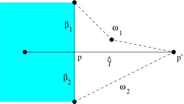
Figure 1. Case IIa.

Case IIb Both endpoints of $\gamma$ lie in $K$. Let $\gamma$ successively cross $\partial K$ at $p_{1},p_{2}$, and let $\gamma_{1}$ be the segment of $\gamma$ lying in the exterior of $K$ between $p_{1}$ and $p_{2}$.

The first case is where $p_{1},p_{2}$ lie on different $\beta_{1},\beta_{2}$ which have endpoints $q_{1}^{1},q_{1}^{2}$ and $q_{2}^{1},q_{2}^{2}$. Then $p_{1},p_{2}$ divide $\beta_{i}$ into segments $\beta_{i}^{\prime},\beta_{i}^{\prime\prime}$. We can form a homotopy class $\beta_{1}^{\prime}*\gamma_{1}*\beta_{2}^{\prime}$ joining $q_{1}^{1}$ to $q_{2}^{2}$ and a homotopy class $\beta_{1}^{\prime\prime}*\gamma_{1}*\beta_{2}^{\prime\prime}$ joining $q_{1}^{2}$ to $q_{2}^{1}$. cWe replace these with their geodesics with the same endpoints and then together with $\beta_{1},\beta_{2}$ they bound a simply connected domain. We are then in a situation similar to Case IIa. See Figure 2.

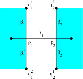
Figure 2. First subcase of Case IIb.

The last case is that $p_{1},p_{2}$ lie on the same saddle connections $\beta$ of $\partial K$. Let $\hat{\beta}$ be the segment between $p_{2}$ and $p_{1}$. Let $\beta_{1}$ and $\beta_{2}$ be the segments joining the endpoints $q_{1},q_{2}$ of $\beta$ to $p_{1},p_{2}$. Find the geodesic in the homotopy class of $\beta_{1}*\gamma_{1}*\beta_{2}$ joining $q_{1}$ to $q_{2}$ and the geodesic in the class of the loop $\beta_{1}*\gamma_{1}*\beta_{2}*\beta^{-1}$ from $q_{1}$ to itself. These two geodesics together with $\beta$ bound a simply connected domain. The analysis is similar to the previous cases. See Figure 3.

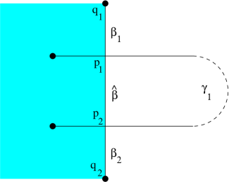
Figure 3. Second subcase of Case IIb.

∎

Now fix the base surface $q$. All angles and lengths will be measured on the base surface. We shall often let $K$ denote a complex equipped with a triangulation without explicit mention the choice of triangulation, as in the statement and proof of Lemma 3.6.

Definition 3.5.

Denote by $L(K)$ the length of the longest saddle connection in $K$. Let $\theta(K)$ the angle that makes the longest saddle connection vertical.

We assume that the complexes considered now have the property that for any saddle connection $\gamma\in K$ we have $|\theta_{\gamma}-\theta(K)|\leq\frac{\pi}{4}$. This implies that measured with respect to the angle $\theta(K)$ we have $|\gamma|=v(\gamma)$. In other words the vertical component is larger than the horizontal component. This will exclude at most finitely many complexes from our game and these will be excluded in any case by our choice of $c_{M+1}$ in Theorem 4.1.

Definition 3.6.

We say a complex $K$ is $\epsilon$-shrinkable if for all saddle connections $\beta$ of $K$ if we let $h(\beta)$ be the component of the holonomy vector in the direction perpendicular to the direction $\theta(K)$ of the longest saddle connection, then $h(\beta)\leq\frac{\epsilon^{2}}{L(K)}$.

We note that this condition could equally well be stated as follows. For any saddle connection $\beta$ of $K$ we have $|\theta_{\beta}-\theta(K)|\leq\frac{\epsilon^{2}}{|\beta|L(K)}$.

The following is immediate.

Lemma 3.7.

If $\epsilon_{1}<\epsilon_{2}$ and $K$ is $\epsilon_{1}$-shrinkable, then it is $\epsilon_{2}$-shrinkable.

Definition 3.7.

A complex $K$ and a saddle connection $\gamma$ that intersects the exterior of $K$ are jointly $\epsilon$-shrinkable if $K$ is $\epsilon$-shrinkable and

• if $|\gamma|\leq L(K)$ then $|\theta(K)-\theta_{\gamma}|\leq\frac{\epsilon^{2}}{|\gamma|L(K)}$.

• if $L(K)<|\gamma|$ then $|\theta_{\gamma}-\theta_{\omega}|\leq\frac{\epsilon^{2}}{|\gamma||\omega|}$ for all $\omega\in K$.

The next lemma says that if the longest saddle connections of each of two complexes have comparable lengths and the angles between these saddle connections is not too large, then the complexes can be combined to form another shrinkable complex.

Lemma 3.8.

Let $K_{1}$ and $K_{2}$ be $\varepsilon$-shrinkable complexes of level $i$ satisfying

$$\left|\theta(K_{1})-\theta(K_{2})\right|<\frac{\rho_{1}\varepsilon^{2}}{L(K_{1})L(K_{2})}\quad\text{ and }\quad L(K_{1})\leq L(K_{2})<\rho_{2}L(K_{1})$$

for some $\rho_{1}>3$ and $\rho_{2}>3$ and assume they are topologically distinct. Then there is an $\varepsilon^{\prime}$-shrinkable complex $K^{\prime}$ of one level higher satisfying $L(K^{\prime})<\rho^{\prime}_{2}L(K_{1})$ where

(4) $$\varepsilon^{\prime}=(16\rho_{1}\rho^{\prime}_{2})^{1/2}\varepsilon\quad\text{ and }\quad\rho^{\prime}_{2}=\sqrt{4\rho_{2}^{2}+9\rho_{1}^{2}\varepsilon^{4}/L(K_{1})^{4}}.$$

Proof.

By Lemma 3.1 there is a saddle connection $\gamma\in K_{2}$ such that $\gamma\not\subset K_{1}$. Let $\theta=\theta(K_{1})$ and $t=\log(L(K_{1})/\varepsilon)$. Then

$$\left|\theta(K_{1})-\theta_{\gamma}\right|<\frac{\rho_{1}\varepsilon^{2}}{L(K_{1})L(K_{2})}+\frac{\varepsilon^{2}}{|\gamma|L(K_{2})}<\frac{2\rho_{1}\varepsilon^{2}}{|\gamma|L(K_{1})}$$

so that

$$h_{\theta}(\gamma)\cdot\frac{L(K_{1})}{\varepsilon}<2\rho_{1}\varepsilon\quad\text{ and }\quad v_{\theta}(\gamma)\cdot\frac{\varepsilon}{L(K_{1})}<\rho_{2}\varepsilon.$$

We apply Lemma 3.6 to produce a new saddle connection $\sigma$. On $g_{t}r_{\theta}X$ we have $\sigma_{\theta,t}=g_{t}r_{\theta}\sigma$ satisfies

$$h(\sigma_{\theta,t})<(2\rho_{1}+3)\varepsilon<3\rho_{1}\varepsilon\quad\text{ and }\quad v(\sigma_{\theta,t})<(\rho_{2}+3)\varepsilon<2\rho_{2}\varepsilon$$

which implies that

$$|\sigma| =\sqrt{\left(h(\sigma_{\theta,t})\cdot\frac{\varepsilon}{L(K_{1})}\right)^{2}+\left(v(\sigma_{\theta,t})\cdot\frac{L(K_{1})}{\varepsilon}\right)^{2}}$$

$$<\sqrt{(3\rho_{1}\varepsilon^{2}/L(K_{1}))^{2}+4\rho_{2}^{2}L(K_{1})^{2}}=\rho^{\prime}_{2}L(K_{1})$$

so that $K^{\prime}=K\cup\{\sigma\}$ satisfies

(5) $$L(K^{\prime})=\max(L(K_{1}),|\sigma|)<\rho^{\prime}_{2}L(K_{1}).$$

If $|\sigma|<L(K_{1})$ we have $K^{\prime}$ is $\varepsilon^{\prime}$-shrinkable because

$$\left|\theta(K_{1})-\theta_{\sigma}\right|\leq 2\frac{h_{\theta}(\sigma)}{|\sigma|}\leq\frac{6\rho_{1}\varepsilon^{2}}{|\sigma|L(K_{1})}$$

while if $|\sigma|\geq L(K_{1})$ it follows that $K^{\prime}$ is $\varepsilon^{\prime}$-shrinkable because $\theta(K^{\prime})=\theta_{\sigma}$ and for every $\xi\in K_{1}$

$$\left|\theta(K^{\prime})-\theta_{\xi}\right| \leq\left|\theta_{\sigma}-\theta(K_{1})\right|+\left|\theta(K_{1})-\theta_{\xi}\right|$$

$$<\frac{6\rho_{1}\varepsilon^{2}}{|\sigma|L(K_{1})}+\frac{\varepsilon^{2}}{|\xi|L(K_{1})}<\frac{6\rho_{1}\varepsilon^{2}}{|\xi|L(K_{1})}<\frac{6\rho_{1}\rho^{\prime}_{2}\varepsilon^{2}}{|\xi|L(K^{\prime})}$$

where $|\sigma|\geq L(K_{1})\geq|\xi|$ and (5) were used in last two inequalities. ∎

The following symmetric version allows us to bypass Lemma 3.1.

Lemma 3.9.

Let $K_{1}$ and $K_{2}$ be $\varepsilon$-shrinkable complexes of level $i$ satisfying

$$\left|\theta(K_{1})-\theta(K_{2})\right|<\frac{\rho_{1}\varepsilon^{2}}{L(K_{1})L(K_{2})}\quad\text{ and }\quad\rho_{2}^{-1}L(K_{1})\leq L(K_{2})<\rho_{2}L(K_{1})$$

for some $\rho_{1}>3$ and $\rho_{2}>3$ and assume they are topologically distinct. Then there is an $\varepsilon^{\prime}$-shrinkable complex $K^{\prime}$ of one level higher satisfying $L(K^{\prime})<\rho^{\prime}_{2}L(K_{1})$ where

(6) $$\varepsilon^{\prime}=(8\rho_{*}\rho^{\prime}_{2})^{1/2}\varepsilon,\quad\rho^{\prime}_{2}=\sqrt{4\rho_{2}^{2}+9\rho_{*}^{2}\varepsilon^{4}/L(K_{1})^{4}}\quad\text{ and }\quad\rho_{*}=\max(\rho_{1},\rho_{2}).$$

Proof.

The only place where $L(K_{1})\leq L(K_{2})$ was used in the previous proof was at the last inequality in the first displayed line. The entire proof goes through if every occurrence of $\rho_{1}$ is replaced with $\rho_{*}$. ∎

In what follows we will be considering shrinkable complexes. In each combinatorial equivalence class of such shrinkable complexes we will consider the complex $K$ which minimizes $L(\cdot)$ and the corresponding angle $\theta(\cdot)$. We note that this complex is perhaps not unique and so there is ambiguity in $\theta(K)$ but this will not matter.

We let $L(\partial K)$ denote the length of the longest saddle connection on the boundary of $K$. We also let $\theta(\partial K)$ the angle that makes the longest vertical.

4. Proofs of Theorem 1.5 and Theorem 4.1

We are now ready to begin the proof of Theorem 1.5. It is based on Theorem 4.1 whose statement and proof were suggested in the outline.

Theorem 4.1.

For all $\beta$ sufficiently small and given Bob’s first move $I_{1}$ in the game, there exist positive constants $c_{i}$, $i=1,\ldots,M+1$, and a strategy for Alice such that regardless of the choices $I_{j}$ made by Bob, the following will hold. For all $\beta c_{i}$-shrinkable level $i$-complexes $K$ if

$$L(K)L(\partial K)|I_{j}|<c_{i}^{2},$$

then

$$d(\theta(K),I_{j})>\frac{\beta c_{i}^{2}}{4L(K)L(\partial K)}.$$

Proof.

We assume $\beta<1/12$. (The value $1/12$ is chosen so that some inequalities that appear in the proof are satisfied). Let $L_{0}$ denote the length of the shortest saddle connection on $(X,q)$. Let $0<c_{1}<\dots<c_{M+1}$ be given by

$$c_{i}=\beta^{N_{i}}c_{i+1}$$

and

$$c_{M+1}=\min(L_{0}\beta^{N_{M}},L_{0}|I_{1}|^{1/2}\varepsilon_{0}),$$

where $N_{i}$ are defined recursively by $N_{1}=6$ and $N_{i+1}=6+2(N_{1}+\dots+N_{i})$. (Again the value $6$ is chosen only so that a particular inequality is satisfied) . These $N_{i}$ are chosen so that

(7) $$\frac{c_{i+1}}{c_{i}}=\beta^{-6}\left(\frac{c_{i}}{c_{1}}\right)^{2}.$$

We remark that this last equation will be used in Step $2$ of the proof. All that is needed is an inequality, but to simplify matters we present it as an equality.

Let $\mathcal{E}_{i}$ be the set of all marked $\beta c_{i}$-shrinkable complexes of level $i$. Given $I_{j}$, we let

$$\mathcal{A}_{i}(j):=\left\{K\in\mathcal{E}_{i}:d(\theta(K),I_{j})>\frac{\beta c_{i}^{2}}{4L(K)L(\partial K)}\right\}$$

and

$$\Omega_{i}(j):=\left\{K\in\mathcal{E}_{i}\setminus\mathcal{A}_{i}(j):\frac{c_{i}^{2}}{L(K)L(\partial K)}\leq|I_{j}|<\frac{\beta^{-1}c_{i}^{2}}{L(K)L(\partial K)}\right\}$$

and

$$z_{i}(j):=\frac{\inf\Theta_{i}(j)+\sup\Theta_{i}(j)}{2}\quad\text{ where }\quad\Theta_{i}(j)=\{\theta(K):K\in\Omega_{i}(j)\}.$$

Alice chooses $M$ intervals of length $\beta|I_{j}|$ centered at the points $z_{i}(j),\;i=1,\dots,M$.

The restatement of theorem then is that for every $j\geq 1$:

($$P_{j} \forall i\in\{1,\dots,M\}\;\forall K\in\mathcal{E}_{i}\qquad L(K)L(\partial K)|I_{j}|<c_{i}^{2}\;\;\Longrightarrow\;\;K\in\mathcal{A}_{i}(j)$$)

Note that ($P_{j}$) holds for all $j<j_{0}:=\min\{k:|I_{k}|<\beta^{2N_{M}}\}$ because

$$L(K)L(\partial K)|I_{j}|\geq L_{0}^{2}\beta^{2N_{M}}\geq c_{M+1}^{2}>c_{i}^{2}$$

while if $j_{0}=1$, we note that $L(K)L(\partial K)|I_{1}|\geq L_{0}^{2}|I_{1}|\geq c_{M+1}^{2}>c_{i}^{2}.$

We proceed by induction and suppose that $j\geq j_{0}$ and that ($P_{j-1}$) holds.

Step 1. For any $K\in\Omega_{i}(j)$,

(8) $$\frac{L(K)}{L(\partial K)}<\beta^{-2}\left(\frac{c_{i}}{c_{1}}\right)^{2}.$$

Consider first the case

(9) $$L(\partial K)^{2}|I_{j}|<\beta c_{1}^{2}.$$

Then $L(\partial K)^{2}|I_{j-1}|<c_{1}^{2}$ so that ($P_{j-1}$) implies the longest saddle connection on $\partial K$ belongs to $A_{1}(j-1)$, meaning

(10) $$d(\theta(\partial K),I_{j-1})>\frac{\beta c_{1}^{2}}{4L(\partial K)^{2}}.$$

But since $K$ is $\beta c_{i}$-shrinkable and not in $\mathcal{A}_{i}(j)$, the triangle inequality implies

$$d(\theta(\partial K),I_{j-1}) \leq\left|\theta(\partial K)-\theta(K)\right|+d(\theta(K),I_{j})$$

$$\leq\frac{\beta^{2}c_{i}^{2}}{L(K)L(\partial K)}+\frac{\beta c_{i}^{2}}{4L(K)L(\partial K)}\leq\frac{\beta c_{i}^{2}}{L(K)L(\partial K)}$$

which together with (10) and the fact that $\beta<\frac{1}{3}$ implies (8). Suppose then that (9) does not hold. Then we have

$$\frac{L(K)}{L(\partial K)}=\frac{L(K)L(\partial K)|I_{j}|}{L(\partial K)^{2}|I_{j}|}<\frac{\beta^{-1}c_{i}^{2}}{\beta c_{1}^{2}}$$

so that (8) holds in this case as well.

Step 2. Any pair $K_{1},K_{2}\in\Omega_{i}(j)$ are topologically equivalent.
For any $K_{1},K_{2}\in\Omega_{i}(j)$, we have

(11) $$\frac{L(K_{2})}{L(\partial K_{1})}<\beta^{-1}\frac{L(K_{1})}{L(\partial K_{2})}.$$

Multiplying (11) by $L(K_{2})/L(\partial K_{1})$ and invoking (8), we get

$$\frac{L(K_{2})}{L(\partial K_{1})}<\beta^{-5/2}\left(\frac{c_{i}}{c_{1}}\right)^{2}$$

so that, exploiting $2<\beta^{-1/2}$, and the above inequality we have

$$\left|\theta(K_{1})-\theta(K_{2})\right|\leq 2|I_{j}|<\frac{2\beta^{-1}c_{i}^{2}}{L(K_{1})L(\partial K_{1})}<\frac{\beta^{-4}(c_{i}/c_{1})^{2}c_{i}^{2}}{L(K_{1})L(K_{2})}.$$

On the other hand again multiplying (11) by $L(K_{2})/L(K_{1})$ and applying (8), we obtain

$$\left(\frac{L(K_{2})}{L(K_{1})}\right)^{2}<\beta^{-1}\frac{L(K_{2})L(\partial K_{1})}{L(\partial K_{2})L(K_{1})}<\beta^{-3}\left(\frac{c_{i}}{c_{1}}\right)^{2}.$$

Now suppose $K_{1}$ and $K_{2}$ are topologically distinct. We shall derive a contradiction. Without loss of generality, we may assume $L(K_{1})\leq L(K_{2})$. The hypotheses of Lemma 3.8 are then satisfied with the parameters

$$\varepsilon=c_{i},\qquad\rho_{1}=\beta^{-4}\left(\frac{c_{i}}{c_{1}}\right)^{2},\quad\text{ and }\quad\rho_{2}=\beta^{-2}\left(\frac{c_{i}}{c_{1}}\right).$$

Consider the two terms under the radical in the expression for $\rho^{\prime}_{2}$ in (4). Note that the second being dominated by the first is equivalent to $L(K_{1})^{2}>\displaystyle\frac{3\rho_{1}}{2\rho_{2}}c_{i}^{2}$. we have

$$|I_{j}|\leq|I_{j_{0}}|<\beta^{2N_{M}}=\left(\frac{c_{M}}{c_{M+1}}\right)^{2}<\left(\frac{c_{1}}{c_{i}}\right)^{4}<\frac{2\rho_{2}}{3\rho_{1}},$$

the first inequality a conseqeunce of (7). Since $L(K_{1})^{2}\geq L(K_{1})L(\partial K_{1})\geq c_{i}^{2}/|I_{j}|$, it now follows that

$$\rho^{\prime}_{2}<3\rho_{2}.$$

Also, since $\rho_{1}=\rho_{2}^{2}$ and $\beta^{2}c_{i+1}=\rho_{2}^{2}c_{i}$, we have

(12) $$\varepsilon^{\prime}=(8\rho_{1}\rho^{\prime}_{2})^{1/2}c_{i}<2\sqrt{6}\rho_{2}^{3/2}c_{i}<\frac{\beta c_{i+1}}{\sqrt{6\rho_{2}}}<\beta c_{i+1}$$

where we used $\beta<1/12$ in the middle inequality.

By Lemma 3.8, there exists a $\beta c_{i+1}$-shrinkable complex $K^{\prime}$ of level $i+1$ satisfying

$$L(K^{\prime})<3\rho_{2}L(K_{1}).$$

Since there are no $c_{M+1}$-shrinkable complexes of level $M+1$, we have our desired contradiction when $i=M$. For $i<M$, we have

$$L(K^{\prime})L(\partial K^{\prime})|I_{j-1}|<\frac{9\rho_{2}^{2}L(K_{1})^{2}|I_{j}|}{\beta}<\frac{9\rho_{2}^{2}c_{i}^{2}L(K_{1})}{\beta^{2}L(\partial K_{1})}<9\beta^{-8}c_{i}^{2}\left(\frac{c_{i}}{c_{1}}\right)^{4}<c_{i+1}^{2},$$

where in the last inequality we have used (7) and (8). The induction hypothesis ($P_{j-1}$) implies $K^{\prime}\in\mathcal{A}_{i+1}(j-1)$, meaning

$$d(\theta(K^{\prime}),I_{j-1})>\frac{\beta c_{i+1}^{2}}{4L(K^{\prime})L(\partial K^{\prime})}\geq\frac{\beta c_{i+1}^{2}}{4L(K^{\prime})^{2}}.$$

On the other hand by (12), $K^{\prime}$ is in fact $\displaystyle\frac{\beta c_{i+1}}{\sqrt{6\rho_{2}}}$-shrinkable, and since $c_{i+1}>\sqrt{6\rho_{2}}c_{i}$, we have

$$d(\theta(K^{\prime},I_{j-1}) \leq\left|\theta(K^{\prime})-\theta(K_{1})\right|+d(\theta(K_{1}),I_{j})$$

$$<\frac{\beta^{2}c_{i+1}^{2}}{6\rho_{2}L(K^{\prime})L(K_{1})}+\frac{\beta c_{i}^{2}}{L(K_{1})L(\partial K_{1})}<\frac{\beta c_{i+1}^{2}}{12\rho_{2}L(K^{\prime})L(K_{1})}<\frac{\beta c_{i+1}^{2}}{4L(K^{\prime})^{2}}$$

which contradicts the previously displayed inequality. This finishes the proof of Step 2.

Step 3. For each $i=1,\dots,M$, we have $\operatorname{diam}\Theta_{i}(j)<\frac{\beta}{2}|I_{j}|$.
Assume $\Omega_{i}(j)\neq\emptyset$ and fix a complex $K_{0}$ in it. The previous step implies for any $K\in\Omega_{i}(j)$, we have $\partial K=\partial K_{0}$. Moreover, the longest saddle connection on $\partial K_{0}$ belongs to $K$ so that since $K$ is $\beta c_{i}$-shrinkable, we have (using $\beta<1/5$)

$$\left|\theta(K)-\theta(\partial K_{0})\right|<\frac{\beta^{2}c_{i}^{2}}{L(K)L(\partial K_{0})}=\frac{\beta^{2}c_{i}^{2}}{L(K)L(\partial K)}<\frac{\beta}{5}|I_{j}|.$$

Thus, $\Theta_{i}(j)$ is inside a ball of radius $\frac{\beta}{5}|I_{j}|$, so that its diameter is $\leq\frac{2\beta}{5}|I_{j}|<\frac{\beta}{2}|I_{j}|$.

Step 4. We now show that ($P_{j}$) holds.
Suppose $K\in\mathcal{E}_{i}$ is such that $L(K)L(\partial K)|I_{j}|<c_{i}^{2}$. Since $|I_{j}|\geq\beta|I_{j-1}|$, we have $L(K)L(\partial K)|I_{j-1}|<\beta^{-1}c_{i}^{2}$. There are two cases. If $L(K)L(\partial K)|I_{j-1}|<c_{i}^{2}$, then ($P_{j-1}$) implies $K\in\mathcal{A}_{i}(j-1)\subset\mathcal{A}_{i}(j)$ and we are done. Otherwise, we conclude that $K\in\Omega_{i}(j-1)$ so that, by the previous step, $\theta(K)$ lies in an interval of length $<\frac{\beta}{2}|I_{j-1}|$ centered about $z_{i}(j-1)$. Since Bob’s interval $I_{j}$ must be disjoint from the interval of length $\beta|I_{j-1}|$ centered at $z_{i}(j-1)$ chosen by Alice, we have

$$d(\theta(K),I_{j})>\frac{\beta}{4}|I_{j-1}|>\frac{\beta c_{i}^{2}}{4L(K)L(\partial K)}.$$

In any case, we have $K\in\mathcal{A}_{i}(j)$. ∎

Proof of Theorem 1.5.

By Theorem 4.1 we are able to ensure that for any level $i$ complex $K_{i}$, we have

$$\max\{L(\partial K)\cdot L(K)\cdot|I_{j}|,L(\partial K)\cdot L(K)\cdot d(\theta(K),I_{j})\}>\frac{\beta c_{i}^{2}}{4}.$$

In particular this holds when $i=1$. Since there is only one saddle connection in a 1-complex, and since for any fixed saddle connection $\gamma$, $|\gamma|^{2}|I_{j}|\to 0$ as $j\to\infty$, we conclude that for all but finitely many intervals $I_{j}$ we have

$$|\gamma|^{2}d(\theta_{\gamma},I_{j})=\max\{|\gamma|^{2}|I_{j}|,|\gamma|^{2}d(\theta_{\gamma},I_{j})\}>\frac{\beta c_{1}^{2}}{4}.$$

Thus if $\phi=\cap_{l=-1}^{\infty}I_{l}$ is the point we are left with at the end of the game, and $\gamma$ is a saddle connection, then $|\gamma|^{2}|\theta_{\gamma}-\phi|>\frac{\beta c_{1}^{2}}{4}$, which by Proposition LABEL:equiv_cond establishes Theorem 1.5. ∎

5. Playing the Game in the Stratum

In this section we prove a theorem that as a corollary will imply Theorem 1.2, Theorem 1.3, Theorem 1.4 and Theorem 1.1. In the general situation we will be playing the game in a subset of a stratum $Q^{1}(k_{1},\ldots,k_{n},\pm)$. In the case of Theorem 1.2 it will be the entire stratum. In the case of Theorem 1.3 and Theorem 1.1 it is the entire space of quadratic differentials on a fixed Riemann surface, and in the case of Theorem 1.4 a subset of the space of Abelian differentials on a compact Riemann surface. What these examples have in common is that there is a $S^{1}$ action on the space given by $q\to e^{i\theta}q$. This will allow us to use the ideas of the previous section.

5.1. Product structure and metric

Given a quadratic differential $q_{0}$ that belongs to a stratum $Q^{1}(k_{1},\ldots,k_{n},\pm)$ and a triangulation $\Gamma=\{e_{i}\}_{i=1}^{6g-6+3n}$ of it, we have a chart $\varphi:U\to\mathbb{C}^{6g-6+3n}$ on a neighborhood $U$ of $q_{0}$ in the stratum where the triangulation remains defined, i.e. none of the triangles are degenerate.

For sufficiently small $U$, using holonomy coordinates, we obtain an embedding

$$\varphi_{\Gamma}:U\to\mathbb{C}^{6g-6+3n}$$

whose image is a convex subset of a linear subspace. Equip $U$ with the metric induced by the norm $\|\boldsymbol{z}\|_{\Gamma}=\max(|z_{1}|,\dots,|z_{6g-6+3n}|)$. Note that the notation $\|q_{1}-q_{2}\|_{\Gamma}$ for the distance between $q_{1}$ and $q_{2}$ in these holonomy coordinates should not be confused with the possibility that $q_{1},q_{2}$ are quadratic differentials on the same Riemann surface in which case $q_{1}-q_{2}$ will refer to vector space subtraction and $\|q_{1}-q_{2}\|$ the area.

We note that $U$ and the induced metric depend only on the $6g-6+3n$ homotopy classes relative to the zeroes of the saddle connections in the triangulation. However a change in homotopy classes will induce a bi-Lipschitz map of metrics and since winning is invariant under bi-Lipschitz maps, we are free to choose any triangulation.

Note that multiplication by $e^{i\theta}$ defines an $S^{1}$-action that is equivariant with respect to $(U,\varphi)$. Let $\pi_{a}:\varphi(U)\to S^{1}$ be the map that gives the argument of $e_{1}$. Let $Z=\pi_{a}^{-1}(\theta_{0})$ where $\theta_{0}=\pi_{a}(q_{0})$ and let $\pi_{Z}:\varphi(U)\to Z$ be the map that sends $q$ to the unique point of $Z$ that is contained in the $S^{1}$-orbit of $q$. Then

$$\varphi(U)\simeq Z\times S^{1}$$

with projections given by $\pi_{Z}$ and $\pi_{a}$.

The metric on $Z$ is the ambient metric:

$$d_{Z}(q_{1},q_{2})=\|q_{1}-q_{2}\|_{\Gamma}\quad\text{ for }\quad q_{1},q_{2}\in Z$$

The metric on $U$ is given by

$$d_{U}(q_{1},q_{2})=\max(d_{Z}(\pi_{Z}(q_{1}),\pi_{Z}(q_{2})),d_{a}(\pi_{a}(q_{1}),\pi_{a}(q_{2})))$$

where $d_{a}(\cdot,\cdot)$ is the distance on $S^{1}$ measuring difference in angles. This metric has the property that a ball in the metric $d_{U}$ is a ball in each factor.

Definition 5.1.

By an $\varepsilon$-perturbation of $q$ we mean any flat surface in $U$ whose distance from $q$ is at most $\varepsilon$.

We now show that the holonomy of any any saddle connection of $q$ is not changed much by an $\varepsilon$-perturbation. Recall the constant $\lambda_{2}$, given in Lemma 3.3 that depends on the and the choice of triangulation.

Lemma 5.1.

Let $q^{\prime}$ be an $\varepsilon$-perturbation of $q$ and suppose that the homotopy class specified by a saddle connection $\gamma$ in $q$ is represented on $q^{\prime}$ by a union of saddle connections $\cup_{1}^{k}\gamma^{\prime}_{i}$. Then the total holonomy vector $hol(\cup\gamma^{\prime}_{i})$ makes an angle at most $2\lambda_{2}\varepsilon$ with the direction of $\gamma$ and and its length differs from that of $\gamma$ by a factor between $1\pm\lambda_{2}\varepsilon$. Also, the direction of the individual $\gamma^{\prime}_{i}$ also lie within $2\lambda_{2}\epsilon$ of $\gamma$.

Proof.

Represent $\gamma$ as a path in the triangulation $\Gamma$ on $q$. After perturbation, the total holonomy vectors $hol(\gamma),hol(\gamma^{\prime})$ satisfy

$$hol(\gamma^{\prime})-hol(\gamma)\leq|\gamma|_{\Gamma}\varepsilon\leq\lambda_{2}|\gamma|\varepsilon,$$

by Lemma 3.3. Hence the difference in angle is at most

$$\arcsin\left(\frac{\lambda_{2}\varepsilon|\gamma|}{|\gamma|}\right)\leq 2\lambda_{2}\varepsilon,$$

proving the first statement.

For the individual $\gamma^{\prime}_{i}$, fix a linear parametrization $q_{t},0\leq t\leq 1$, so that $q_{0}=q$ and $q_{1}=q^{\prime}$. Then there are times $0=t_{0}<t_{1}<\dots<t_{n}=1$ and saddle connections $\gamma_{j}$ on $q_{t_{j}}$ (that are parallel to other saddle connections on $q_{t_{j}}$) such that $\gamma_{0}=\gamma$, $\gamma_{n}=\gamma^{\prime}_{i}$, and, by the first part of the lemma, the angle between $\gamma_{j}$ and $\gamma_{j+1}$ is at most

$$2\lambda_{2}\varepsilon(t_{j+1}-t_{j}).$$

The triangle inequality now implies the angle between the holonomies of $\gamma$ and $\gamma^{\prime}_{i}$ is at most $2\lambda_{2}\varepsilon$. ∎

5.2. Moving complexes

In the proof of the theorems we will need to move triangulations from one quadratic differential to another in order to play the games. In such a move, vertices of the triangulation may hit other edges forcing degenerations. The following theorem is the mechanism for keeping track of complexes as they move. We first note that about each point in the stratum there is a neighborhood where the homotopy class of a saddle connection can be consistently defined.

Theorem 5.1.

Suppose $q_{t};0\leq t\leq 1$ is a smooth path of quadratic differentials in a given stratum. Suppose $K$ is a complex on $q_{0}$ (with triangulation $\Gamma$). Then there is a complex $K^{\prime}$ on $q_{1}$ with triangulation, denoted $\Gamma^{\prime}$ and a piecewise linear map $F:K\to K^{\prime}$ such that

1. the homotopy class of every saddle connection of $K$ is mapped by $F$ to a union of saddle connections on $K^{\prime}$. These saddle connections have the same homotopy class.

2. the closed subset $K^{\prime}$ depends only on $K$ and the path of quadratic differentials; in particular it does not depend on the choice of triangulation of $\Gamma$ of $K$.

Proof.

Let $T$ be the set of $t\geq 0$ such that the geodesic representative on $q_{t}$ of the homotopy class of each saddle connection in $\Gamma$ is realized by a single saddle connection in $q_{t}$. Let $A(0)$ be the connected component of $T$ containing $0$. For each $t\in A(0)$, let $\Gamma_{t}$ be the collection of saddle collections in $q_{t}$ representing these homotopy classes. It is easy to see that $\Gamma_{t}$ is a pairwise disjoint collection and that three saddle connections in $\Gamma$ bound a triangle if and only if the corresponding saddle connections in $\Gamma_{t}$ bound a triangle. Let $K_{t}$ be the complex determined by $\Gamma_{t}$. The obvious piecewise linear map $f_{t}:K\to K_{t}$ is a homeomorphism onto its image.

Let $t_{1}=\sup A(0)$. We claim that the closed set $K_{t}$ is independent of the choice of triangulation $\Gamma$ for $0<t<t_{1}$. Indeed, suppose $\tilde{\Gamma}$ is another triangulation of $K$ such that for $0<t<t_{1}$ the geodesic representative on $q_{t}$ of the homotopy class of each saddle connection in $\tilde{\Gamma}$ is realized by a single saddle connection on $q_{t}$. Let $\tilde{f}_{t}:K\to\tilde{K}_{t}$ be the simplicial homeomorphism between $K$ and the complex $K_{t}$ determined by the corresponding collection $\tilde{\Gamma}_{t}$ of saddle connections on $q_{t}$. Then $\tilde{f}_{t}$ and $f_{t}$ agree on $\partial K$, so that $\partial K_{t}=f_{t}(\partial K)=\tilde{f}_{t}(\partial K)=\partial\tilde{K}_{t}$. Note that $f_{t}$ and $\tilde{f}_{t}$ induce the same transverse orientation on any saddle connection in $\partial K_{t}$. Since $\tilde{f}_{t}\circ f_{t}^{-1}$ restricts to the identity on $\partial K_{t}$, it maps each connected component of the interior of $K_{t}$ to itself. Hence, the interiors of $K_{t}$ and $\tilde{K}_{t}$ coincide, and therefore $K_{t}=\tilde{K}_{t}$, proving the claim.

Let $(E,\pi:E\to[0,t_{1}])$ be the pull-back of the tautological bundle so that each fiber $\pi^{-1}(t)$ is a copy of $q_{t}$ for each $t\in[0,t_{1}]$. Let $\Omega\subset E$ be the subset that intersects each fiber in $K_{t}$. Define $K_{t_{1}}=\bar{\Omega}\setminus\Omega$ and note that it is a closed set contained in the fiber over $t=t_{1}$. Let $f_{t_{1}}:K\to K_{t_{1}}$ be the pointwise limit of the maps $f_{t}$ as $t\to t_{1}^{-}$. Each saddle connection $\gamma$ of $\Gamma$ is mapped by $f_{t_{1}}$ to a union of parallel saddle connections $\gamma^{\prime}_{i},i=1,\dots,r=r(\gamma)$. A triangle $\Delta$ determined by $\Gamma$ may collapse under $f_{t_{1}}$ to a union of parallel saddle connections; otherwise, $f_{t_{1}}(\Delta)$ has $n=n(\Delta)$ saddle connections on its boundary, possibly with $n>3$. If $n>3$, then $n-3$ zeroes of $q_{t}$ hit the interior of an edge of $\Delta$ at $t=t_{1}$. In this case we triangulate $f_{t_{1}}(\Delta)$ by adding $n-3$ ”extra” saddle connections. Let $\Gamma_{t_{1}}$ be the collection of saddle connections $\gamma^{\prime}_{i}$ associated to $\gamma\in\Gamma$ together with the “extra” saddle connections needed to triangulate $f_{t_{1}}(\Delta)$ for $\Delta$ that do not collapse and have $n(\Delta)>3$. Let $K^{\prime}_{t_{1}}$ be the complex determined by $\Gamma_{t_{1}}$ and let $f^{\prime}_{t_{1}}:K\to K_{t_{1}}^{\prime}$ be the composition of $f_{t_{1}}$ with the inclusion of $K_{t_{1}}$ into $K^{\prime}_{t_{1}}$. It is easy to see that $F_{t_{1}}:=f^{\prime}_{t_{1}}$ maps saddle connections to unions of saddle connections and that $K^{\prime}_{t_{1}}$ does not depend on the choice of $\Gamma$.

If $t_{1}=1$ we are done and we set $K^{\prime}=K^{\prime}_{t_{1}}$. Thus assume $t_{1}<1$. We repeat the construction above starting with $K^{\prime}_{t_{1}}$ and form the maximal set $A(t_{1})$ of times $t_{1}\leq t<t_{2}$ such that the homotopy class of each saddle connection of $K^{\prime}_{t_{1}}$ is realized by a single saddle connection on $q_{t}$. We repeat the procedure, building a new complex $K^{\prime}_{t_{2}}$ and finding a map $f^{\prime}_{2}:K^{\prime}_{t_{1}}\to K^{\prime}_{t_{2}}$. We then let $F_{t_{2}}=F_{1}\circ f^{\prime}_{t_{1}}$. The compactness of $[0,1]$ implies that this procedure only need be repeated a finite number of times $t_{1}<t_{2}<\dots<t_{N}=1$. We inductively find $F_{t_{N}}$ and set $F=F_{t_{N}}$ and $K^{\prime}=K^{\prime}_{t_{N}}$. ∎

Definition 5.2.

Let $q^{\prime}$ be an $\varepsilon$-perturbation of $q$ and $K$ a complex in $q$. Let $K^{\prime}$ be the complex obtained by applying Theorem 5.1 using the linear path in the stratum joining $q$ and $q^{\prime}$. We call $K^{\prime}$ the moved complex.

Corollary 5.1.

Let $q^{\prime}$ be an $\varepsilon$-perturbation of $q$ and suppose that $K$ is a complex on $q$ that moves to $K^{\prime}$ on $q^{\prime}$ by $F$. Let $\gamma\in K$. Let $\cup_{1}^{k}\gamma_{i}^{\prime}=F(\gamma)$. Then $|\theta_{\gamma}-\theta_{\gamma_{i}^{\prime}}|<2\lambda_{2}\varepsilon$.

Proof.

Each $f^{\prime}_{t_{k}},i=1,\dots,N$ in the proof of Theorem 5.1 is a piecewise linear map between complexes on $q_{k}$ that are $\varepsilon_{k}$-perturbations of one another, where $\sum_{k=1}^{N}\varepsilon_{k}=\varepsilon$. Let $\sigma_{k},k=0,1,\dots,N$ be the saddle connections such that $\sigma_{0}=\gamma$, $f^{\prime}_{t_{k}}(\sigma_{k-1})\supset\sigma_{k}$, and $\sigma_{N}=\gamma^{\prime}_{i}$. Lemma 5.1 implies $|\theta_{k-1}-\theta_{k}|<2\lambda_{2}\varepsilon_{k}$ where $\theta_{k}$ denotes the direction of $\sigma_{k}$. The conclusion of the corollary now follows from the triangle inequality. ∎

Proposition 2.

Suppose $K_{1}\subset K_{2}$ as closed subsets and each is a complexes on $q_{0}$. They are both moved to $q_{1}$ to become complexes $K_{1}^{\prime},K_{2}^{\prime}$. Then again viewed as closed subsets, we have $K_{1}^{\prime}\subset K_{2}^{\prime}$.

Proof.

We can extend the triangulation of $K_{1}$ to a triangulation $\hat{K}_{1}$ of the same closed subset as is defined by $K_{2}$ and such that $\hat{K}_{1}$ and $K_{2}$ coincide on the boundary. We move both $K_{2}$ and $\hat{K}_{1}$ to $q_{1}$ obtaining triangulations $K_{2}^{\prime}$ and $\hat{K}_{1}^{\prime}$. Theorem 5.1 says that $K_{2}^{\prime}$ and $\hat{K}_{1}^{\prime}$ are triangulations of the same closed set. Clearly $K_{1}^{\prime}\subset\hat{K}_{1}^{\prime}$ and we are done. ∎

We adopt the notation $(K,q)$ to refer to a complex on the flat surface defined by $q$.

Definition 5.3.

Suppose $(K_{1},q_{1})$ and $(K_{2},q_{2})$ are complexes of distinct flat surfaces. We say $(K_{1},q_{1})$ and $(K_{2},q_{2})$ are not combinable if $K_{1}$ moved to $q_{2}$ satisfies $K_{1}^{\prime}\subseteq K_{2}$ and $K_{2}$ moved to $q_{1}$ satisfies $K_{2}^{\prime}\subseteq K_{1}$. Otherwise they are said to be combinable.

5.3. Proof of Theorem 1.2

We are given the compact set $\bar{U}$ in the stratum. For any $\alpha,\beta$ we can play the game a finite number of steps so that we are allowed to assume that $U$ is a ball with center $q_{0}$ which has a triangulation $\Gamma$ which remains defined for all $q\in U$. We are therefore able to talk about $\epsilon$ perturbations in $U$. Furthermore since $\bar{U}$ is compact, the constant $\lambda_{2}$ given by Lemma 3.3 which depends only on the and the triangulation can be taken to be uniform in $U$. Furthermore because our choice of metric is the sup metric, each ball $B_{j}$ will be of the form

$$B_{j}=Z_{j}\times I_{j},$$

where $Z_{j}$ is a ball in the space $Z$ and $I_{j}\subset S^{1}$.

Now choose

(13) $$\alpha<\min\{\frac{1}{8},\frac{1}{720(6g-6+n)^{2}\lambda_{2}}\},$$

where $n$ is the number of zeroes. (Again the significance of the choice of constants $8$, $720$ is only to make certain inequalities hold.) Let $L_{0}$ denote the length of the shortest saddle connection on $q_{0}$. Let $0<c_{1}<\dots<c_{M+1}$ be given by $c_{i}=(\alpha\beta)^{N_{i}}c_{i+1}$ and

$$c_{M+1}=\min(L_{0}\beta^{N_{M}},L_{0}|I_{1}|^{1/2}\varepsilon_{0})$$

where $N_{i}$ are defined by $N_{1}=4M+1$ and $N_{i+1}=4M+4(N_{1}+\dots+N_{i})$ so that

(14) $$\frac{c_{i+1}}{c_{i}}=(\alpha\beta)^{-4M-1}\left(\frac{c_{i}}{c_{1}}\right)^{4}\geq 100(\alpha\beta)^{-4M}\left(\frac{c_{i}}{c_{1}}\right)^{4}.$$

Now inductively, given a ball $B_{j}=Z_{j}\times I_{j}$, where $Z_{j}$ is centered at $q_{j}$, let $\mathcal{E}_{i}(B_{j}):=\mathcal{E}_{i}$ be the set of all marked $(\alpha\beta)^{3+M}c_{i}$-shrinkable complexes $(K,q)$ of level $i$ where $q\in B_{j}$. Given $I_{j}$ with $j\equiv M-i+1$ mod $M$, we let

$$\mathcal{A}_{i}(j):=\left\{(K,q)\in\mathcal{E}_{i}:d(\theta(K),I_{j})>\frac{(\alpha\beta)^{M}c_{i}^{2}}{24L(K)L(\partial K)}\right\}.$$

We shall prove the following statement for every $j\geq 1$ and every $i\in\{1,\dots,M\}$, where $j\equiv M-i+1$ mod $M$.

($$P_{j} \;\forall K\in\mathcal{E}_{i}\qquad L(K)L(\partial K)|I_{j}|<c_{i}^{2}\;\;\Longrightarrow\;\;K\in\mathcal{A}_{i}(j)$$)

Note that ($P_{j}$) holds automatically for all $j<j_{0}:=\min\{k:|I_{k}|<\beta^{2N_{M}}\}$ because

$$L(K)L(\partial K)|I_{j}|\geq L_{0}^{2}\beta^{2N_{M}}\geq c_{M+1}^{2}>c_{i}^{2}$$

while if $j_{0}=1$, we note that $L(K)L(\partial K)|I_{1}|\geq L_{0}^{2}|I_{1}|\geq c_{M+1}^{2}>c_{i}^{2}.$

We proceed by induction and suppose that Alice is given a ball $B_{j}=Z_{j}\times I_{j}$, $j\geq j_{0}$, where $Z_{j}\subset Z$ is a ball and $I_{j}\subset I$ is an interval. Suppose inductively that ($P_{k}$) holds for $k\leq j$. We will show that Alice has a choice of a ball $A_{j}\subset B_{j}$ to ensure $(P_{j+M})$ will hold.

Define

$$\Omega_{i}(j):=\left\{(K,q)\in\mathcal{E}_{i}\setminus\mathcal{A}_{i}(j):\frac{c_{i}^{2}}{L(K)L(\partial K)}\leq|I_{j}|<\frac{(\alpha\beta)^{-M}c_{i}^{2}}{L(K)L(\partial K)}\right\}.$$

We summarize our strategy. We will show that for any $q_{1},q_{2}\in B_{j}$ such that $d_{U}(q_{1},q_{2})\leq\alpha|B_{j}|$, no two complexes $(K_{1},q),(K_{2},q)$ are combinable (step 2). Then we will show that if $d_{U}(q^{\prime},q)\leq\alpha|Z_{j}|$, and $(K,q),(K^{\prime},q^{\prime})\in\Omega_{i}(j)$ are complexes which are not pairwise combinable, then $|\theta(K)-\theta(K^{\prime})|$ is small (step 3). Then choosing some $(K,q)$, Alice can choose an angle $\phi$ where $d(\phi,\theta(K))>\frac{1}{3}|I_{j}|$, and an interval $I_{j}^{\prime}$ centered at $\phi$ of radius $\alpha|I_{j}|$. There will be no $(K^{\prime},q^{\prime})$ with $\theta(K^{\prime})\in I_{j}^{\prime}$ and where $K^{\prime}$ is combinable with $K$ and $d_{U}(q,q^{\prime})\leq\alpha|Z_{j}|$ (step 4). As in the proof of Theorem 4.1, step 1 is a technical result controlling the ratio of $L(K)$ and $L(\partial K)$, which is necessary for step 2.

Step 1. We show that for any $(K,q)\in\Omega_{i}(j)$,

(15) $$\frac{L(K)}{L(\partial K)}<(\alpha\beta)^{-2M}\left(\frac{c_{i}}{c_{1}}\right)^{2}.$$

This is essentially the same as the proof of Step 1 in the proof of Theorem 4.1. We provide the details. Let $k$ be the previous stage for dealing with 1-complexes. Consider first the case that

(16) $$L(\partial K)^{2}|I_{j}|<(\alpha\beta)^{M}c_{1}^{2}.$$

Then $L(\partial K)^{2}|I_{k}|<c_{1}^{2}$ so that ($P_{k}$) implies the longest saddle connection on $\partial K$ belongs to $A_{1}(k)$, meaning

$$d(\theta(\partial K),I_{k})>\frac{(\alpha\beta)^{M}c_{1}^{2}}{24L(\partial K)^{2}}>c_{1}^{2}|I_{k}|.$$

But since $K$ is $(\alpha\beta)^{3+M}c_{i}$-shrinkable and not in $\mathcal{A}_{i}(j)$, the triangle inequality implies

$$d(\theta(\partial K),I_{j}) \leq\left|\theta(\partial K)-\theta(K)\right|+d(\theta(K),I_{j})$$

$$\leq\frac{(\alpha\beta)^{6+2M}c_{i}^{2}}{L(K)L(\partial K)}+\frac{(\alpha\beta)^{M}c_{i}^{2}}{24L(K)L(\partial K)}\leq\frac{(\alpha\beta)^{M}c_{i}^{2}}{L(K)L(\partial K)}$$

which implies (15) using the fact that $\alpha\beta<1$. Suppose now that (16) does not hold. Since $(K,q)\in\Omega_{i}(j)$, we have

$$\frac{L(K)}{L(\partial K)}=\frac{L(K)L(\partial K)|I_{j}|}{L(\partial K)^{2}|I_{j}|}<\frac{(\alpha\beta)^{-M}c_{i}^{2}}{(\alpha\beta)^{M}c_{1}^{2}}$$

so that (15) holds in this case as well.

Step 2. Now we show that if $(K_{1},q_{1})$ and $(K_{2},q_{2})$ are in $\Omega_{i}(j)$ and

$$d_{U}(q_{1},q_{2})\leq\alpha|B_{j}|,$$

then $K_{1}$ and $K_{2}$ are not combinable. Assume on the contrary that they are combinable. So without loss of generality assume there exists $\gamma\in K_{2}$ so that the moved $\gamma^{\prime}\not\subset K_{1}$.

Choose the following constants.

Let $\varepsilon=c_{i}(\alpha\beta)^{3+M},\qquad\rho_{1}=2(\alpha\beta)^{-4M}\left(\frac{c_{i}}{c_{1}}\right)^{2},\quad\rho_{2}=(\alpha\beta)^{-2M}\left(\frac{c_{i}}{c_{1}}\right)$ and  $\rho_{3}=12\rho_{2}(\rho_{1}+\rho_{2})$.

We now show that we can combine $\gamma^{\prime}$ to $K_{1}$ to make a $\sqrt{\rho_{3}}\epsilon$-shrinkable complex. Observe that similarly to the proof of Step 2 in Theorem 4.1 we have

$$|\theta(K_{1})-\theta(K_{2})|\leq(1+\frac{1}{12})|B_{j}|\leq\frac{\rho_{1}\epsilon^{2}}{L(K_{1})L(K_{2})}\text{ and }\frac{L(K_{1})}{L(K_{2})}\leq\rho_{2}.$$

Therefore

(17) $$|\theta_{\gamma^{\prime}}-\theta(K_{1})|\leq|\theta_{\gamma}-\theta_{\gamma^{\prime}}|+|\theta_{\gamma}-\theta(K_{2})|+|\theta(K_{1})-\theta(K_{2})|\leq\\ \lambda_{2}\|q_{1}-q_{2}\|+\frac{3\epsilon^{2}}{2|\gamma^{\prime}|L(K_{2})}+\frac{\rho_{1}\epsilon^{2}}{L(K_{1})L(K_{2})}\leq\frac{2\epsilon^{2}}{|\gamma^{\prime}|L(K_{2})}+\frac{2\rho_{1}\epsilon^{2}}{L(K_{1})L(K_{2})}\leq\frac{(2\rho_{1}+2\rho_{2})\epsilon^{2}}{|\gamma^{\prime}|L(K_{1})}$$

Let $\theta=\theta(K_{1})$ and $t=\log\frac{(L(K_{1})}{\epsilon}$. There is a saddle connection $\sigma$ disjoint from $K_{1}$ such that on $g_{t}r_{\theta}X$ the saddle connection $\sigma_{\theta,t}=g_{t}r_{\theta}\sigma$ satisfies

$$h_{\theta}(\sigma_{\theta,t})\leq(2\rho_{2}+2\rho_{1}+3)\epsilon\text{ and }v_{\theta}(\sigma_{\theta,t})\leq\frac{3}{2}\rho_{2}\epsilon.$$

It follows that

$$|\sigma|\leq\sqrt{\left(\frac{(2\rho_{2}+2\rho_{1}+3)\epsilon}{L(K_{1})}\right)^{2}+\left(\frac{3\rho_{2}L(K_{1})}{2}\right)^{2}}\leq 2\rho_{2}L(K_{1}).$$

Now we show $\hat{K}=K_{1}\cup\sigma$ is $\epsilon\sqrt{\rho_{3}}$ shrinkable. We have $L(\hat{K})=\max\{L(K_{1}),|\sigma|\}$. If $L(\hat{K})=L(K_{1})$ then $\hat{K}$ is $\epsilon\sqrt{\rho_{3}}$ shrinkable because

$$|\theta_{\sigma}-\theta(K_{1})|\leq 2\frac{h_{\theta}(\sigma)}{|\sigma|}\leq\frac{(5\rho_{1}+5\rho_{2})\epsilon^{2}}{|\sigma|L(K_{1})}.$$

If $L(\hat{K})=|\sigma|$ for every $\xi\in K_{1}$ we have

$$\left|\theta(\hat{K})-\theta_{\xi}\right| \leq\left|\theta_{\sigma}-\theta(K_{1})\right|+\left|\theta(K_{1})-\theta_{\xi}\right|$$

$$<\frac{(5\rho_{1}+5\rho_{2})\varepsilon^{2}}{|\sigma|L(K_{1})}+\frac{\varepsilon^{2}}{|\xi|L(K_{1})}<\frac{(6\rho_{1}+6\rho_{2})\varepsilon^{2}}{|\xi|L(K_{1})}<\frac{(12\rho_{1}+12\rho_{2})\rho_{2}\varepsilon^{2}}{|\xi|L(\hat{K})}$$

where $2\rho_{2}L(K_{1})\geq|\sigma|\geq L(K_{1})\geq|\xi|$ was used in last two inequalities. This shows that $\hat{K}$ is $\sqrt{\rho_{3}}\epsilon$-shrinkable.

Now we derive a contradiction. Notice that $c_{i+1}(\alpha\beta)^{3+M}>\sqrt{\rho_{3}}\epsilon$ and so $\hat{K}$ is $c_{i+1}(\alpha\beta)^{3+M}$ shrinkable.

Since there are no $c_{M+1}$-shrinkable complexes of level $M+1$, we have our desired contradiction when $i=M$. For $i<M$, we have

$$L(\hat{K})L(\partial\hat{K})|B_{j-1}|<\frac{4\rho_{2}^{2}L(K_{1})^{2}|B_{j}|}{\alpha\beta}<\frac{4\rho_{2}^{2}c_{i}^{2}L(K_{1})}{(\alpha\beta)^{1+M}L(\partial K_{1})}<4(\alpha\beta)^{-7M-1}c_{i}^{2}\left(\frac{c_{i}}{c_{1}}\right)^{4}<c_{i+1}^{2}.$$

The first inequality uses the bound on $L(\hat{K})$ in terms of $L(K_{1})$ and the definition of the game. The third inequality uses Step 1. We conclude that the induction hypothesis ($P_{j-1}$) implies $\hat{K}\in\mathcal{A}_{i+1}(j-1)$, meaning

(18) $$d_{a}(\theta(\hat{K}),I_{j-1})>\frac{(\alpha\beta)^{M}c_{i+1}^{2}}{24L(\hat{K})L(\partial\hat{K})}\geq\frac{(\alpha\beta)^{M}c_{i+1}^{2}}{24L(\hat{K})^{2}}.$$

Since $\hat{K}$ is $\sqrt{\rho_{3}}\epsilon$ shrinkable by the choice of $\epsilon$, it is in fact ${c_{i}\sqrt{\rho_{3}}(\alpha\beta)^{M}}$-shrinkable, and since ${c_{i+1}>c_{i}\sqrt{\rho_{3}}\sqrt{4(\alpha\beta)^{-M}\rho_{2}}}$, we have

$$d_{a}(\theta(\hat{K}),I_{j-1})\leq\left|\theta(\hat{K})-\theta(K_{1})\right|+d_{a}(\theta(K_{1}),I_{j})\leq\frac{\rho_{3}(\alpha\beta)^{M}c_{i}^{2}}{L(K_{1})L(\hat{K})}+\frac{(\alpha\beta)^{M}}{24L(K_{1})L(\partial K_{1})}\\ <\frac{2\rho_{3}\rho_{2}(\alpha\beta)^{M}c_{i}^{2}}{L(\hat{K})^{2}}+\frac{(\alpha\beta)^{M}2\rho_{2}\rho_{2}\rho_{1}c_{i}^{2}}{L(\hat{K})^{2}}<\frac{(\alpha\beta)^{M}c_{i+1}^{2}}{24L(\hat{K})^{2}}$$

giving us the desired contradiction to (18).

Step 3. We show that if $(K_{1},q_{1})$ is not combinable with $(K_{2},q_{2})$, each belongs to $\Omega_{i}(j)$, and $d_{U}(q_{1},q_{2})\leq 2\alpha|B_{j}|$, then $|\theta(K_{1})-\theta(K_{2})|\leq\frac{1}{3}|B_{j}|$.

Since $(K_{1},q_{1})$ and $(K_{2},q_{2})$ are not combinable, when we move $K_{1}$ to $q_{2}$ which we denote by $K_{1}^{\prime}$, we have $K_{1}^{\prime}\subseteq K_{2}$. Similarly $K_{2}^{\prime}\subset K_{1}$. By Proposition 2 when we move $K_{1}^{\prime}$ back to $q_{1}$, denoted by $K_{1}^{\prime\prime}$, we have

$$K_{1}^{\prime\prime}\subset K_{2}^{\prime}\subset K_{1}.$$

But since each saddle connection on $\partial K_{1}$ is homotopic to a union of saddle connections of $K_{1}^{\prime\prime}$ with common endpoints, $K_{1}$ and $K_{1}^{\prime\prime}$ bound a union of (possibly degenerate) simply connected domains each of which has a segment of $\partial K_{1}$ as a side. Let $\gamma$ be the longest saddle connection on $\partial K_{1}$ and let $\Delta$ be the corresponding simply connected domain. Since $K_{1}^{\prime\prime}\subset K_{2}^{\prime}\subset K_{1}$, $\Delta$ contains a union of saddle connections $\hat{\kappa}^{\prime}\subset\partial K_{2}^{\prime}$ that join the endpoints of $\gamma$. Let $p\leq 6g-6+n$ denote the cardinality of $\hat{\kappa}^{\prime}$.

Since $d_{U}(q_{1},q_{2})\leq 2\alpha|B_{j}|$, each is a $2\alpha|B_{j}|$ perturbation of the other. Since the angle the saddle connections of $\partial K_{2}$ make with each other goes to $\pi$ as the length of the segments goes to $\infty$, and these angles change by a small factor, by Corollary 5.1 we have for some $\kappa^{\prime}\in\hat{\kappa}^{\prime}$,

(19) $$L(\partial K_{1})\leq 2p|\kappa^{\prime}|.$$

and for all $\kappa^{\prime}\in\hat{\kappa}^{\prime}$,

(20) $$|\kappa^{\prime}|\leq pL(\partial K_{1}).$$

Since lengths change by a factor of at most $1+\lambda_{1}\leq\frac{3}{2}$ in moving, and since $\kappa^{\prime}$ arises from a saddle connection $\kappa\subset\partial K_{2}$, we have that

$$L(\partial K_{1})\leq 3p|\kappa|\leq 3pL(\partial K_{2}),$$

and by symmetry

$$L(\partial K_{2})\leq 3rL(\partial K_{1}),$$

for some constant $r\leq 6g-6+n$, so that

(21) $$|\kappa^{\prime}|\geq\frac{L(\partial K_{2})}{9rp}\geq\frac{L(\partial K_{2})}{9(6g-6+3n)^{2}}.$$

We also claim that

$$|\theta_{\kappa^{\prime}}-\theta(K_{1})|<\frac{1}{20}|B_{j}|.$$

To see this, by Corollary 5.1 applied twice, first to the moved $K_{1}^{\prime}$ and then to $K_{1}^{\prime\prime}$, and by the choice of $\alpha$, in (13), we have that for all $\gamma^{\prime}\in\partial\Delta$

$$|\theta_{\gamma^{\prime}}-\theta_{\gamma}|\leq\frac{1}{40}|B_{j}|,$$

which implies since $\kappa^{\prime}$ is a union of saddle connections in $\Delta$ that

$$|\theta_{\gamma}-\theta_{\kappa^{\prime}}|\leq\frac{1}{40}|B_{j}|.$$

The shrinkability of $K_{1}$ implies that

$$|\theta(K_{1})-\theta_{\gamma}|\leq\frac{c_{i}^{2}(\alpha\beta)^{2M}}{L(K_{1})|\gamma|}\leq\frac{1}{40}|B_{j}|,$$

so the claim follows from the last two inequalities.

By Corollary 5.1, the triangle inequality, and the above claim we have

$$|\theta(K_{1})-\theta(K_{2})|\leq|\theta(K_{1})-\theta_{\kappa^{\prime}}|+|\theta_{\kappa^{\prime}}-\theta_{\kappa}|+|\theta_{\kappa}-\theta(K_{2})|\leq\frac{1}{20}|B_{j}|+\frac{1}{40}|B_{j}|+|\theta(K_{2})-\theta_{\kappa}|.$$

By our shrinkability assumption on $K_{2}$,

$$|\theta_{\kappa}-\theta(K_{2})|\leq\frac{c_{i}^{2}(\alpha\beta)^{2M}}{L(K_{2})|\kappa|}\leq\frac{1}{20}|B_{j}|,$$

where the second inequality follows from (21), the definition of $\Omega_{i}(j)$, and the choice of $\alpha$ given in (13). Step 3 follows.

Step 4.

Bob presents Alice with a ball $B_{j}=Z_{j}\times I_{j}$ where $j\equiv M-i+1$ mod $M$. If there is no $(K,q)$ in $\Omega_{i}(j)$, Alice makes an arbitrary move. Otherwise, pick a $(K,q)\in\Omega_{i}(j)$. Alice chooses a ball ${A_{j}=Z_{j}^{\prime}\times I_{j}^{\prime}}$ of diameter $\alpha|B_{j}|$, whose center has first coordinate $q$ and second coordinate is as far from $\theta(K,q)$ as possible. Observe that

$${d_{a}(\theta(K,q),I_{j})^{\prime}\geq(\frac{1}{2}-2\alpha)|B_{j}|}.$$

By Step 2 if $\hat{q}\in Z_{j}$ and $(\hat{K},\hat{q})\in\Omega_{i}(j)$ then $\hat{K}$ and $K$ are not combinable. By Step 3

$$d(\theta(\hat{K},\hat{q}),I_{j}^{\prime})\geq(\frac{1}{2}-2\alpha)|B_{j}|-\frac{1}{3}|B_{j}|\geq(\frac{1}{6}-2\alpha)|B_{j}|.$$

Now because $(\hat{K},\hat{q})\in\Omega_{i}(j)$, using the left hand inequality in the definition and that $\alpha\beta<1$, we conclude that

$$d_{a}(\theta(\hat{K},\hat{q}),I_{j}^{\prime})\geq(\frac{1}{6}-2\alpha)\frac{c_{i}^{2}(\alpha\beta)^{M}}{L(\hat{K})L(\partial\hat{K})}.$$

Because $d_{a}(\theta,I_{j}^{\prime})\leq d_{a}(\theta,I_{j+M}^{\prime})$ we know then that $(P_{j+M})$ holds. This finishes the inductive proof of $(P_{j})$.

We finish the proof of Theorem  1.2. By $(P_{j})$ we are able to ensure that for any level $i$ complex $K$ on a surface $q$, we have

$$\max\{L(\partial K)\cdot L(K)\cdot|B_{j}|,L(\partial K)\cdot L(K)\cdot d_{\theta}((q,K),B_{j}\}>\frac{(\alpha\beta)^{M}c_{i}^{2}}{4}.$$

In particular this holds when $i=1$. Since there is only one saddle connection in a 1-complex, and since for any fixed saddle connection $\gamma$ on a surface $q$, $|\gamma|^{2}|B_{j}|\to 0$ as $j\to\infty$, we conclude that for all but finitely many balls $B_{j}$ we have

$$|\gamma|^{2}d_{\theta}((q,\gamma),B_{j})=\max\{|\gamma|^{2}|B_{j}|,|\gamma|^{2}d_{\theta}((q,\gamma),B_{j}\}>\frac{(\alpha\beta)^{M}c_{1}^{2}}{4}.$$

Thus if $(q,\phi)=\cap_{l=-1}^{\infty}B_{l}$ is the point we are left with at the end of the game, and $\gamma$ is a saddle connection on $q$, then $|\gamma|^{2}|\theta_{\gamma}-\phi|>\frac{(\alpha\beta)^{M}c_{1}^{2}}{4}$, which by Proposition LABEL:equiv_cond establishes the statement of strong winning in Theorem 1.2.

The set cannot be absolute winning for the following reason. Bob begins by choosing a ball $I_{1}$ centered at some quadratic differential which has a vertical saddle connection $\gamma$. The set $X_{\gamma}$ consisting of quadratic differentials with a vertical saddle connection $\gamma$ is a closed subset of codimension one and such quadratic differentials are clearly not bounded. Then whatever Alice’s move of a ball $J_{1}\subset I_{1}$, Bob can find a next ball $I_{2}\subset I_{1}\setminus J_{1}$ centered at some new point in $X_{\gamma}$ which shows that bounded quadratic differentials are not absolute winning.

An identical proof allows us the same theorem in the case of marked points.

Theorem 5.2.

Let $Q$ be a stratum of quadratic differential with $k$ marked points. Let $U\subset Q$ be an open set with compact closure in $Q$ where the metric given by local coordinates is well defined. The set $E\subset\bar{U}$ consisting of those quadratic differentials $q$ such that the Teichmüller geodesic defined by $q$ stays in a compact set in the stratum is $\alpha$ winning for Schmidt’s game. In fact it is $\alpha$-strong winning.

In fact with a similar proof we have the following

Theorem 5.3.

Let $P$ be a rotation invariant subset of the stratum of quadratic differentials with $k$ marked points where a metric given by local coordinates is well defined. Assume $P$ has compact closure in the stratum. The set $E\subset P$ consisting of those quadratic differentials $q$ such that the Teichmüller geodesic defined by $q$ stays in a compact set in the stratum is $\alpha$ winning for Schmidt’s game. In fact it is $\alpha$-strong winning.

5.4. Proof of Theorem 1.1

Again as before the Diophantine foliations are not absolute winning since for any closed curve $\gamma$ the set of foliations $F$ such that $i(F,\gamma)=0$ is a codimension one subset.

We now show strong winning. We can assume we start with a fixed train track $\tau$, and a small ball $B(F_{0},r)$ of foliations carried by $\tau$. Indeed, if the initial ball Bob chooses contains points on the boundary of two or more charts, then Alice can use the strategy of choosing her balls furthest away from these boundary points, so that in a finite number of steps her choice will be contained in a single chart.

By choosing transverse foliations, we can insure that there a ball $B^{\prime}(q_{0},r^{\prime})\subset Q^{1}(1,\ldots,1,-)$ of quadratic differentials contained in the principal stratum so that

• the vertical foliation of each $q\in B^{\prime}(q_{0},r^{\prime})$ is in $B(F_{0},r)$.

• each vertical foliation in $B(F_{0},r)$ is the vertical foliation of some $q\in B(q_{0},r^{\prime})$.

• $B(F_{0},r)$ and $B^{\prime}(q_{0},r^{\prime})$ are small enough so that the holonomies of a fixed set of saddle connections serve as local coordinates.

• There is a fixed constant so that the holonomy of any $q\in B^{\prime}(q_{0},r^{\prime})$ is bounded away from $0$ by that constant.

In holonomy coordinates the map that sends $q\in B^{\prime}(q_{0},r^{\prime})$ to its vertical foliation is just projection onto the horizontal coordinates. This map clearly satisfies the hypotheses of Theorem 2.1. Since the bounded geodesics form a strong winning set in $Q^{1}(1,\ldots,1,-)$ by Theorem 1.2 they are strong winning in $\mathcal{PMF}$.

5.5. Proof of Theorem 1.4

If the condition $\inf_{n}n|T^{n}(p_{1})-p_{2}|>0$ holds for any pair of discontinuities $p_{1},p_{2}$ of $T$, we say $T$ is badly approximable. The following lemma connects the badly approximated condition for interval exchanges with the bounded condition for geodesics.

Lemma 5.2.

(Boshernitzan [1, Pages 748-750]) $T$ is badly approximable if and only if the Teichmüller geodesic corresponding to vertical direction is bounded for any zippered rectangle such that $T$ arises as the first return of the vertical flow to a transversal.

See in particular the first equation on page 750, which relates the size of smallest interval bounded by discontinuities of $T^{n}$ and closeness to a saddle connection direction. That is, let $T$ be an IET that arises from first return to a transversal of a flow on a flat surface $q$. Assume that the smallest interval of continuity of $T^{n}$ is less than $\frac{\epsilon}{n}$ then

$$|\theta(v)-\theta|<\frac{C\epsilon}{nL(v)},$$

where $v$ is a saddle connection on $q$ with length $O(n)$. Recall Theorem 1.6 relates closeness to saddle connection directions to boundedness of the Teichmüller geodesics.

We now give the proof of Theorem 1.4. For the same reason as above the set of bounded interval exchanges is not absolute winning. For strong winning, the proof is identical to the one for $\mathcal{PMF}$ except that now, using for example the the zippered rectangle construction, we can assume we have a small ball $B$ in the space of interval exchange transformations [16], a corresponding ball in some stratum $B^{\prime}\subset Q^{1}(k_{1},\ldots,k_{n},+)$, such that each interval exchange transformation in $B$ arises from the first return to a horizontal transversal of some $\omega\in B^{\prime}$, and conversely for each $\omega\in B^{\prime}$, the first return to a horizontal transversal gives rise to a point in $B$. We can assume these transversals vary continuously. Again the map from holonomy coordinates in $B^{\prime}$ to lengths in $B$ is given by projection onto horizontal coordinates. We now apply Lemma 5.2, Theorem 1.2 and Theorem 2.1.

If we mark points $a,b$ in the interval then we have

Theorem 5.4.

Given any irreducible permutation $\pi$ there exists $\alpha>0$ such that for any pair of points $(a,b)$ we have

$$\{T=T_{L,\pi}:\inf_{n>0}\{nd(T^{n}a,b)\}>0\}$$

is an $\alpha$-strong winning set.

Proof.

As in the last theorem we find a ball in the stratum such that first return to transversals give the interval exchange. Now mark the points along each transversal at distances $a,b$ to obtain a set $B^{\prime}$ of marked translation surfaces. It is not a ball but it is invariant under rotations lying in a small interval about the identity. Then by Theorem 5.3 the set of bounded trajectories in it is strong winning. By Theorem 2.1 the image of this set is strong winning in the space of marked interval exchange transformations. ∎

5.6. Proof of Theorem 1.3

Let $U$ be the intersection of the principle stratum with $Q^{1}(X)$. Since the complement of $U$ is contained in a finite union of smooth submanifolds, then for any sufficiently small $\alpha>0$ and for any sufficiently small ball chosen by Bob, Alice can respond with a ball contained entirely in $U$ with the bounded away from zero. Thus, we may assume Bob’s initial ball $B_{1}$ is contained in $U$. By the main theorem of [5], the homeomorphism from $Q^{1}(X)\to\mathcal{PMF}$ sending a quadratic differential to the projective class of its vertical foliation is smooth when restricted to $U$. We can now apply Theorem 1.1.

References

- [1] Boshernitzan, M: A condition for minimal interval exchange maps to be uniquely ergodic. Duke Math. J. 52 (1985), no. 3, 723–752.
- [2] Boshernitzan, M: Rank two interval exchange transformations. Ergod. Th. & Dynam. Sys. 8 (1988), no. 3, 379–394.
- [3] Dani, S. G: Bounded orbits of flows on homogeneous spaces, Comment. Math. Helv. 61 (1986), no. 4, 636–660.
- [4] Fathi, A, Laudenbach, F, Poenaru, V: Travaux de Thurston sur les surfaces Asterisque 66-67 (1979)
- [5] Hubbard, J, Masur, H: Quadratic differentials and foliations, Acta. Math. 1979 142 221-274.
- [6] Kerckhoff, S, Masur, H, Smillie, J: Ergodicity of billiard flows and quadratic differentials, Annals of Math, 1986 124 293-311.
- [7] Kleinbock, D. Y, Margulis, G. A. Bounded orbits of nonquasiunipotent flows on homogeneous spaces. Sinaĭ’s Moscow Seminar on Dynamical Systems, Amer. Math. Soc. Transl. Ser. 2, 171, Amer. Math. Soc., Providence, RI, 1996, pp. 141–172.
- [8] Kleinbock, D, Weiss, B: Bounded geodesics in moduli space. Int. Math. Res. Not. 2004, 30, 1551-1560.
- [9] Kleinbock, D, Weiss, B: Modified Schmidt games and diophantine approximation with weights, Advances in Math. 223 (2010), 1276-1298.
- [10] McMullen, C. T: Winning sets, quasiconformal maps and Diophantine approximation. Geom. Funct. Anal. 2010, 20, 726-740.
- [11] McMullen, C.T: Diophantine and ergodic foliations on surfaces, preprint
- [12] Masur, H, Tabachnikoff, S: Rational billiards and flat structures B.Haselblatt, A.Katok 9ed) Handbook of Dynamical Systems, Elseveir Vol1A 1015-1089 (2002)
- [13] Minsky, Y, Weiss, B: Nondivergence of horocyclic flows on moduli space. I. Reine Angew. Math. (2002), 552, 131-177.
- [14] Penner, R, Harer, J:Combinatorics of train tracks Annals of Math Studies 125 Princeton University Press 1992.
- [15] Schmidt, W: On badly approximable numbers and certain games. Trans. Amer. Math. Soc. 1966 123 178–-199.
- [16] Veech, W: Gauss measures for transformations on the space of interval exchange maps. Ann. of Math. (2) 115 (1982) 201-242.