Local anomalies around the third peak in the CMB angular power spectrum
of the WMAP 7-year data

Abstract

We estimate the power spectra of CMB temperature anisotropy in localized regions on the sky using the WMAP 7-year data. Here, we report that the north hat and the south hat regions at the high Galactic latitude ($|b|\geq 30^{\circ}$) show anomaly in the power spectrum amplitude around the third peak, which is statistically significant up to $3\sigma$. We try to figure out the cause of the observed anomaly by analyzing the low Galactic latitude ($|b|<30^{\circ}$) regions where the galaxy contamination is expected to be stronger, and regions that are weakly or strongly dominated by the WMAP instrument noise. We also consider the possible effect of unresolved radio point sources. We found another but less statistically significant anomaly in the low Galactic latitude north and south regions whose behavior is opposite to the one at the high latitude. Our analysis shows that the observed north-south anomaly at high latitude becomes weaker on the regions with high number of observations (weak instrument noise), suggesting that the anomaly is significant at sky regions that are dominated by the WMAP instrument noise. We have checked that the observed north-south anomaly has weak dependences on the bin-width used in the power spectrum estimation and the Galactic latitude cut. We have also discussed the possibility that the detected anomaly may hinge on the particular choice of the multipole bin around the third peak. We anticipate that the issue of whether the anomaly is intrinsic one or due to the WMAP instrument noise will be resolved by the forthcoming Planck data.

1 Introduction

The cosmic microwave background radiation (hereafter CMB) provides us with a wealth of information on the history of the universe. The thermal black body nature of the CMB energy spectrum is now considered as the firm evidence of the hot big bang scenario for the beginning of the universe (Alpher & Herman 1948; Dicke et al. 1965; Penzias & Wilson 1965). The existence of large-scale structure in the universe also implies that there were primordial density perturbations as the seeds for structure formation. It was expected that these inhomogeneities would have the imprint on the CMB as the minute temperature fluctuations (anisotropy) (Sachs & Wolfe 1967; Peebles & Yu 1970; Bond & Efstathiou 1987). The CMB anisotropy was discovered by the Cosmic Background Explorer (COBE) Differential Microwave Radiometers experiment (Smoot et al. 1992) and has been confirmed by many ground-based and balloon-borne experiments (see Hu & Dodelson 2002; Scott & Smoot 2006 for reviews and references therein).

Recently, the Wilkinson Microwave Anisotropy Probe (WMAP) has opened a new window to the precision cosmology by measuring the CMB temperature anisotropy and polarization with high resolution and sensitivity (Bennett et al. 2003; Jarosik et al. 2011). For every data release, the WMAP team presented their estimation of the angular power spectra for temperature and polarization anisotropy (Hinshaw et al. 2003, 2007; Page et al. 2003, 2007; Nolta et al. 2009; Larson et al. 2011). By comparing the measured CMB power spectra with the theoretical prediction, the WMAP team determined the cosmological parameters with a few % precision (Spergel et al. 2003, 2007; Komatsu et al. 2009, 2011), and found that the observed CMB fluctuations are consistent with predictions of the concordance $\Lambda\textrm{CDM}$ model with scale-invariant adiabatic fluctuations generated during the inflationary epoch (Spergel et al. 2003; Peiris et al. 2003; Komatsu et al. 2011). Recent ground-based and balloon-borne experiments that have performed the CMB power spectrum measurement and the cosmological parameter estimation include the South Pole Telescope (SPT) (Keisler et al. 2011), the QUaD experiment (Brown et al. 2009), Arcminute Cosmology Bolometer Array Receiver (ACBAR) (Reichardt et al. 2009), the Cosmic Background Imager (CBI) (Mason et al. 2003), the Atacama Cosmology Telescope (ACT) (Fowler et al. 2010), the Degree Angular Scale Interferometer (DASI) (Carlstrom et al. 2003), BOOMERANG (Jones et al. 2006), Archeops (Benoît et al. 2003), and MAXIMA (Lee et al. 2001).

In the CMB data analysis the two-point statistics such as the correlation function and the power spectrum has been widely used. In particular, the relation between the CMB angular power spectrum and the cosmological physics is well understood, and the tight constraints on the cosmological parameters can be directly obtained by comparing the measured power spectrum with the theoretical prediction. Therefore, the accurate estimation of the angular power spectrum from the observed CMB maps is the essential step. The efficient techniques to measure the angular power spectrum from the CMB temperature fluctuations with incomplete sky coverage have been constantly developed (e.g., Górski 1994; Tegmark 1997; Bond et al. 1998; Oh et al. 1999; Szapudi et al. 2001; Wandelt et al. 2001; Hansen et al. 2002; Hivon et al. 2002; Mortlock et al. 2002; Hinshaw et al. 2003; Wandelt et al. 2003; Chon et al. 2004; Efstathiou 2004; Eriksen et al. 2004a; Wandelt et al. 2004; Brown et al. 2005; Polenta et al. 2005; Fay et al. 2008; Dahlen & Simons 2008; Das et al. 2009; Mitra et al. 2009; Ansari et al. 2010; Chiang & Chen 2012).

Until now, the analysis of the WMAP CMB data has been made using the whole sky area except for strongly contaminated regions (Hinshaw et al. 2003, 2007; Nolta et al. 2009; Larson et al. 2011; Saha et al. 2006, 2008; Souradeep et al. 2006; Eriksen et al. 2007a; Samal et al. 2010; Basak & Delabrouille 2012). On the other hand, there was only a small number of studies on the power spectrum measurement on the partial regions of the sky (e.g., Eriksen et al. 2004b; Hansen et al. 2004a, b; Ansari et al. 2010; Yoho et al. 2011; Chiang & Chen 2012). Especially, Yoho et al. (2011) detected degree-scale anomaly around the first acoustic peak of the CMB angular power spectrum measured on a small patch of the north ecliptic sky. In this work, we measure the angular power spectra from the WMAP 7-year temperature anisotropy data set on some specified regions of the sky. We found that at high Galactic latitude regions there is the north-south anomaly or asymmetry in the power amplitude around the third peak of the angular power spectrum, which is the main result of this paper. Our result differs from the well-known hemispherical asymmetry in the angular power spectrum and the genus topology at large angular scales (Park 2004; Eriksen et al. 2004b, c, 2007b; Hansen et al. 2004b; Bernui 2008; Hansen et al. 2009; Hoftuft et al. 2009).

This paper is organized as follows. In Sec. 2, we describe the method of how to measure the angular power spectrum. The application of the method to the WMAP 7-year data and the comparison with the WMAP team’s measurement are shown in Sec. 3. In Sec. 4, we measure the power spectra on various sky regions defined with some criteria, and present our discovery of the north-south anomaly around the third peak of the angular power spectrum at high Galactic latitude regions. We also discuss the potential origin of such a north-south anomaly. Section 5 is the conclusion of this work. Throughout this work we have used the HEALPix software (Górski et al. 1999, 2005) to measure the pseudo angular power spectra and to generate the WMAP mock data sets.

2 Angular power spectrum estimation method

In this section we briefly review how the angular power spectrum is measured from the observed CMB temperature anisotropy maps. Throughout this work we do not consider the CMB polarization.

In the ideal situation where the temperature fluctuations on the whole sky are observed, we can expand the temperature distribution $T(\mathbf{n})$ in terms of spherical harmonics as

$$T({\mathbf{n}})=\sum_{l=2}^{\infty}\sum^{l}_{m=-l}a_{lm}Y_{lm}({\mathbf{n}}),$$ (1)

where $\mathbf{n}$ denotes the angular position on the sky, $Y_{lm}(\mathbf{n})$ is the spherical harmonic basis function, and the monopole ($l=0$) and dipole ($l=1$) components have been neglected. From the orthogonality condition of the spherical harmonics, the coefficients $a_{lm}$ can be obtained from

$$a_{lm}=\int d\Omega T({\mathbf{n}})Y^{*}_{lm}({\mathbf{n}}),$$ (2)

where $d\Omega$ denotes the differential solid angle on the sky. If the temperature anisotropy is statistically isotropic, then the variance of the harmonic coefficients $a_{lm}$ is independent of $m$ and the angular power spectrum $C_{l}$ is given as the ensemble average of two-point product of the harmonic coefficients,

$$\langle a_{lm}a^{*}_{l^{\prime}m^{\prime}}\rangle=C_{l}\delta_{ll^{\prime}}\delta_{mm^{\prime}},$$ (3)

where the bracket represents the ensemble average and $\delta_{ll^{\prime}}$ is the Kronecker delta symbol ($\delta_{ll^{\prime}}=1$ for $l=l^{\prime}$, and $\delta_{ll^{\prime}}=0$ for $l\neq l^{\prime}$). For a Gaussian temperature distribution, it is known that all the statistical information is included in the two-point statistics like the angular power spectrum $C_{l}$.

For the single realization of temperature fluctuations on the sky, the ensemble average is replaced with the simple average of independent modes belonging to the same multipole $l$ and the angular power spectrum becomes

$$C_{l}^{\textrm{\scriptsize sky}}=\frac{1}{2l+1}\sum^{l}_{m=-l}|a_{lm}|^{2},$$ (4)

with uncertainty due to the cosmic variance

$$\Delta C_{l}=\sqrt{\frac{2}{2l+1}}C_{l}.$$ (5)

In the practical situation, however, we usually exclude some portion of the sky area where the contamination due to the Galactic emission and the strong radio point sources is expected to affect the statistics of the CMB anisotropy significantly. The limited angular resolution, the instrument noise, and the finite pixels of the processed map also prevent us from using the formulas, Eqs. (1)–(5), which are valid only in the ideal situation. The incomplete sky coverage with an arbitrary geometry and the limited instrumental performance break the orthogonality relation between the spherical harmonic functions. Thus, measuring angular power spectrum from the realistic observational data is more complicated.

There are two popular ways of measuring the angular power spectrum from the observed CMB data with incomplete sky coverage. One is the maximum likelihood estimation method based on the Bayesian theorem (Bond et al. 1998; Tegmark 1997), and the other is the pseudo power spectrum method that applies the Fourier or harmonic transformation directly (Hivon et al. 2002). For the latter, Hivon et al. (2002) developed the so called MASTER (Monte Carlo Apodised Spherical Transform Estimator) method which estimates the angular power spectrum from the high resolution CMB map data. For mega-pixelized data sets like those from WMAP or Planck (Planck Collaboration et al. 2011a), the MASTER method is faster and more efficient than the maximum likelihood method.

We refer to the pseudo angular power spectrum as $\tilde{C_{l}}$ to distinguish from the true angular power spectrum $C_{l}$ which we try to estimate. Two quantities differ from each other due to the incomplete sky coverage, the limited angular resolution and pixel size, and the instrument noise, and they are related by (Hansen et al. 2002; Hivon et al. 2002)

$$\langle\tilde{C_{l}}\rangle=\sum_{l^{\prime}}M_{ll^{\prime}}F_{l^{\prime}}B^{2}_{l^{\prime}}\langle C_{l^{\prime}}\rangle+\langle\tilde{N_{l}}\rangle,$$ (6)

where $B_{l}$ is the beam transfer function, $F_{l}$ is the pixel transfer function due to finite pixel size of the CMB map, $\langle\tilde{N}_{l}\rangle$ is the average pseudo noise power spectrum due to the instrument noise, and $M_{ll^{\prime}}$ is the mode-mode coupling matrix that incorporates all the effect due to the incomplete sky coverage. The mode-mode coupling matrix is written as

$$M_{l_{1}l_{2}}=\frac{2l_{2}+1}{4\pi}\sum_{l_{3}}(2l_{3}+1){\mathcal{W}}_{l_{3}}\left\lgroup\begin{array}[]{ccc}l_{1}&l_{2}&l_{3}\\ 0&0&0\end{array}\right\rgroup^{2},$$ (7)

where ${\mathcal{W}}_{l}$ is the power spectrum of the window function for incomplete sky coverage (see Sec. 3.2), and the last factor on the right-hand side enclosed with the parenthesis represents the Wigner 3-$j$ symbol. We use the Fortran language and the Mathematica software to calculate the Wigner 3-$j$ symbols; see also Hivon et al. (2002) and Brown et al. (2005) for the numerical computation of the Wigner 3-$j$ symbols.

To reduce the statistical variance of the measured angular power spectrum due to the cosmic variance and the instrument noise, we usually average powers within the appropriate $l$ bins. According to Hivon et al. (2002), the binning operator is defined as

$$P_{bl}=\bigg{\{}\begin{array}[]{ll}\frac{1}{2\pi}\frac{l(l+1)}{l^{(b+1)}_{\textrm{\tiny low}}-l^{(b)}_{\textrm{\tiny low}}},&\textrm{if $2\leq l^{(b)}_{\textrm{\scriptsize low}}\leq l<l^{(b+1)}_{\textrm{\scriptsize low}}$}\\ 0,&\textrm{otherwise}.\end{array}$$

The reciprocal operator is defined as

$$Q_{lb}=\bigg{\{}\begin{array}[]{ll}\frac{2\pi}{l(l+1)},&\textrm{if $2\leq l^{(b)}_{\textrm{\scriptsize low}}\leq l<l^{(b+1)}_{\textrm{\scriptsize low}}$}\\ 0,&\textrm{otherwise},\end{array}$$

where $b$ is the bin index. For ease of comparison, we use exactly the same $l$-binning adopted by the WMAP teams ($b$ runs from 1 to 45) (Larson et al. 2011). The true power spectrum can be estimated from

$$\hat{C}_{b}=(K^{-1})_{bb^{\prime}}P_{b^{\prime}l}(\tilde{C}_{l}-\langle\tilde{N}_{l}\rangle),$$ (8)

where

$$K_{bb^{\prime}}=P_{bl}M_{ll^{\prime}}F_{l^{\prime}}B_{l^{\prime}}^{2}Q_{l^{\prime}b^{\prime}}$$ (9)

is a kernel matrix that describes the mode-mode couplings due to the survey geometry, the finite resolution and pixel size, and the binning process.

Ideally the average pseudo noise power spectrum $\langle\tilde{N}_{l}\rangle$ can be estimated by the Monte Carlo simulation that mimics the instrument noise. However, because of the statistical fluctuations in the noise power spectra itself, it is rather difficult to obtain an accurate estimation of the power contribution due to the instrument noise from the single observed data. In our analysis we evade this problem by measuring the cross-power spectra between different channel data sets, in the same way as adopted by the WMAP team (see the next section).

3 Application to the WMAP 7-year data

3.1 WMAP 7-year data

The WMAP mission was designed to make the full sky CMB temperature and polarization maps with high accuracy, precision, and reliability (Bennett et al. 2003). The WMAP instrument has 10 differencing assemblies (DAs) spanning five frequency bands from 23 to 94 GHz: one DA each at 23 GHz (K1) and 33 GHz (Ka1), two DAs each at 41 GHz (Q1, Q2) and 61 GHz (V1, V2), and four DAs at 94 GHz (W1, W2, W3, W4), with $0\hbox{$.\!\!^{\circ}$}82$, $0\hbox{$.\!\!^{\circ}$}62$, $0\hbox{$.\!\!^{\circ}$}49$, $0\hbox{$.\!\!^{\circ}$}33$, and $0\hbox{$.\!\!^{\circ}$}21$ FWHM beam widths, respectively. In this work we use the foreground-reduced WMAP 7-year temperature fluctuation maps that are prepared in the HEALPix format with $N_{\textrm{\scriptsize side}}=512$ (resolution 9; r9). The total number of pixels of each map is $12\times N_{\textrm{\scriptsize side}}^{2}=3,145,728$. Following the WMAP team’s analysis, we use only V and W band maps to reduce any possible contamination due to the Galactic foregrounds. We use the WMAP beam transfer function ($B_{l}$) and the number of observations ($N_{\textrm{\scriptsize obs}}$) for each DA. All the data sets used in this work are available on the NASA’s Legacy Archive for Microwave Background Data Analysis (LAMBDA).

3.2 Weighting schemes

The window function assigns a weight to the temperature fluctuation on each pixel before the harmonic transformation is performed. In our analysis the window function maps have been produced based on two weighting schemes, the uniform weighting scheme and the inverse-noise weighting scheme (Hinshaw et al. 2003). The WMAP team provides mask maps which assigns unity to pixels that are used in the analysis and zero to pixels that are excluded to avoid the foreground contamination. We use the KQ85 mask map with resolution 9 that includes about 78.3% of the whole sky area. The mask map excludes the Galactic plane region with the strong Galactic emission and the circular areas with $0\hbox{$.\!\!^{\circ}$}6$ radius centered on the strong radio point sources. The uniform weighting scheme uses the mask map as the window function directly,

$$W(p)=M(p),$$ (10)

where $M(p)$ denotes a mask map on a pixel $p$ on the sky. The power spectrum at high $l$ region is usually dominated by the instrument noise. In the WMAP data the noise level on each pixel is modeled by

$$\sigma(p)=\frac{\sigma_{0}}{\sqrt{N_{\textrm{\scriptsize obs}}(p)}},$$ (11)

where $N_{\textrm{\scriptsize obs}}(p)$ is the number of observations on the pixel $p$ and $\sigma_{0}$ is the global noise level ($\sigma_{0}=3.319$, $2.955$, $5.906$, $6.572$, $6.941$, $6.778$ mK for V1, V2, W1, W2, W3, W4 DAs, respectively). To reduce the effect of the instrument noise, the inverse-noise weighting scheme is defined as the product of the mask map and the map of number of observations,

$$W(p)=M(p)N_{\textrm{\scriptsize obs}}(p).$$ (12)

The window function at 94 GHz W4 frequency channel (DA) is shown in Fig. 1, together with a histogram of the number of observations. Although the WMAP team applies the uniform weighting scheme for $l<600$ and the inverse-noise weighting scheme for $l>600$ (Larson et al. 2011), in this work we simply apply the single weighting scheme over the whole range of $l$ considered ($2\leq l\leq 1200$) during the power spectrum estimation and compare the results based on the two weighting schemes.

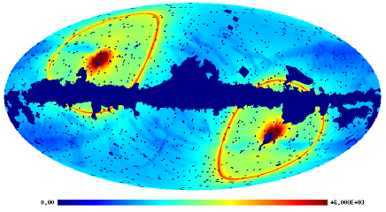
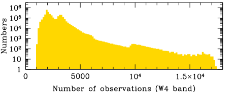
Fig. 1.—: (Top) A map of number of observations $N_{\textrm{\scriptsize obs}}(p)$ at the WMAP 7-year W4 frequency channel (DA), multiplied with the KQ85 mask map $M(p)$ [see Eq. (12)]. Dark blue color corresponds to zero values and represents regions that are excluded by the KQ85 mask map, while dark red color denotes the value exceeding $N_{\textrm{\scriptsize obs}}\geq 6000$. The Mollweide projection in Galactic coordinates is used to display this map, where the Galactic center is located at the center, the Galactic longitude increases from center to left ($l=0^{\circ}$–$180^{\circ}$) and from right to center ($l=180^{\circ}$–$360^{\circ}$), and the Galactic latitude increases from bottom to top ($b=-90^{\circ}$–$+90^{\circ}$). The regions with large number of observations correspond to the ecliptic pole regions. (Bottom) A histogram of number of observations at the same frequency channel.

3.3 Angular power spectrum measured from the WMAP data

In the WMAP team’s data analysis, the power spectrum at low multipoles ($l\leq 32$) was measured by a Blackwell-Rao estimator that is applied to a chain of Gibbs samples obtained from the foreground-cleaned CMB map while the power spectrum at high multipoles ($32<l\leq 1200$) by the MASTER pseudo power spectrum estimation method (Larson et al. 2011). Throughout this work, the angular power spectrum over the whole $l$ range ($2\leq l\leq 1200$) is measured based on the pseudo power spectrum estimation method because our primary attention is paid on the high $l$ region where the peaks are located. Thus, as shown below our results at low multipoles are somewhat different from the WMAP team’s results.

The WMAP V and W bands have two (V1 and V2) and four (W1, W2, W3, and W4) separate frequency channels (DAs). Using the Anafast program in the HEALPix package, we measured 15 pseudo cross power spectra ($\tilde{C}_{l}$) for different channel combinations (V1W1, V1W2, and so on) based on the uniform and the inverse-noise weighting schemes. During the production of each pseudo cross power spectrum, Anafast program estimates two separate sets of harmonic coefficients for each DA using the formula Eq. (2) where $T({\mathbf{n}})$ is now replaced with $W({\mathbf{n}})T({\mathbf{n}})$ and $W({\mathbf{n}})$ is the window function defined in Eqs. (10) and (12) for the corresponding DA. We set the maximum multipole as $l=1200$.

For each channel combination, we calculate the mode-mode coupling matrix $M_{ll^{\prime}}$ and the kernel matrix $K_{bb^{\prime}}$ using the beam transfer, the pixel transfer functions, and the same $l$-binning as defined by the WMAP team (Larson et al. 2011). For the power spectrum of window function in Eq. (7) we use the cross power spectrum of window functions for the corresponding DA combination, which is obtained from the Anafast program by inserting the window functions at two different frequency channels as the input data. The squared beam transfer function $B_{l}^{2}$ appearing in Eq. (6) is also modified into the product of beam transfer functions from the two different frequency channels.

The final binned cross power spectrum $\hat{C}_{b}$ for each channel combination is obtained from Eq. (8) neglecting the term for the average noise power spectrum $\langle\tilde{N}_{l}\rangle$. Since the properties of the instrument noise for each channel are independent, the process of cross-correlation statistically suppresses the contribution of the instrument noise to the power spectrum estimation. This technique has an advantage that our power spectrum estimator is not biased by noise if the noise in the two independent channels is uncorrelated; the cross-correlation between the uncorrelated noise vanishes statistically. Thus, the measured cross-power spectra are independent of instrument noise from the individual channels in every practical sense (see Hinshaw et al. 2003). Note that the self-combination of each frequency channel data (like V1V1, V2V2, W1W1) is not considered during the analysis because it is essentially needed to subtract the contribution of noise power from the measured auto-power spectrum and it is a difficult task to precisely estimate the noise power from the single observed map (see the discussion at the end of Sec. 2). For each binned cross power spectrum we subtract the contribution due to the unresolved radio point sources expected in the WMAP temperature anisotropy maps by using the information presented in Nolta et al. (2009) and Larson et al. (2011). The amplitude of the binned power spectrum due to the unresolved point sources can be written as

$$C_{\textrm{\scriptsize ps},b}^{i}=A_{\textrm{\scriptsize ps}}P_{bl}S_{l}^{i}.$$ (13)

Here $S_{l}^{i}$ is the point-source spectral function given by

$$S_{l}^{i}\equiv r(\nu_{k})r(\nu_{k^{\prime}})\left(\frac{\nu_{k}\nu_{k^{\prime}}}{\nu_{\textrm{\scriptsize Q}}^{2}}\right)^{\beta}$$ (14)

where $\nu_{k}$ and $\nu_{k^{\prime}}$ denote the individual frequency channel belonging to $i$-th channel combination, $r(\nu_{k})$ is a conversion factor from antenna to thermodynamic temperature, $\nu_{\textrm{\scriptsize Q}}=40.7~{}\textrm{GHz}$ is the Q-band central frequency, $10^{3}A_{\textrm{\scriptsize ps}}=9.0\pm 0.7~{}\mu\textrm{K}^{2}$, and $\beta=-2.09$ (see also Huffenberger et al. 2006; Souradeep et al. 2006). The subindex $l$ is dummy because the spectral function does not depend on it.

To combine these cross power spectra into the single angular power spectrum, in fact we need the Monte Carlo simulation data sets with the similar properties of the WMAP observational data. Using the Synfast program of HEALPix and assuming the concordance flat $\Lambda\textrm{CDM}$ model with parameters, $\Omega_{b}h^{2}=0.02260$, $\Omega_{c}h^{2}=0.1123$, $\Omega_{\Lambda}=0.728$, $n_{s}=0.963$, $\tau=0.087$, $\Delta_{\mathcal{R}}^{2}(k=0.002~{}\textrm{Mpc}^{-1})=2.441\times 10^{-9}$ (Table 14 of Komatsu et al. 2011), we have made 1000 mock data sets that mimic the WMAP beam resolution and instrument noise for each channel. We use the CAMB software to obtain the theoretical model power spectrum (Lewis et al. 2000). We assumed that the temperature fluctuations and instrument noise follow the Gaussian distribution. In the simulation data sets we do not consider any effect due to the residual foreground contamination. We have analyzed the one thousand WMAP simulation mock data sets in the same way as the real data set is analyzed.

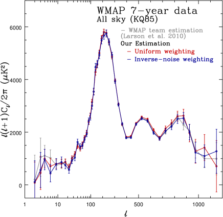
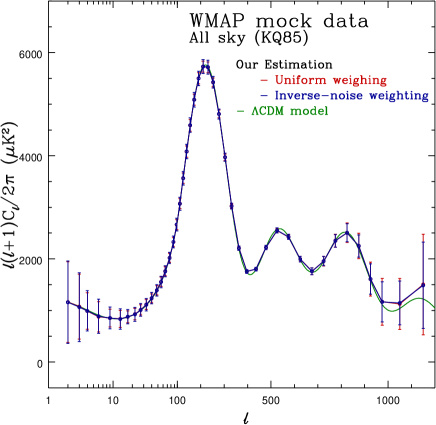
Fig. 2.—: (Left) Angular power spectra measured from the WMAP 7-year temperature anisotropy maps. Our results are shown as red and blue curves with dots and error bars for uniform and inverse-noise weighting schemes, respectively. The sky area (78.27% of the whole sky) defined in the KQ85 mask map has been used. For a comparison, the WMAP team’s result is also shown as grey curve with dots and error bars (Larson et al. 2011). (Right) Averaged angular power spectra measured from the one thousand WMAP mock data sets that are consistent with the concordance $\Lambda\textrm{CDM}$ model (Komatsu et al. 2011). Red color denotes the result based on the uniform weighting scheme while blue based on the inverse-noise weighting scheme. The power spectrum of the assumed concordance $\Lambda\textrm{CDM}$ model is shown as green curve.

Before combining the cross power spectra into the single power spectrum, each cross power spectrum has been averaged within $l$-bins specified to reduce the statistical fluctuations due to the cosmic variance and the instrument noise. We use the same $l$-bins defined by the WMAP 7-year data analysis (Larson et al. 2011). Thus, in a case when we measure the power spectrum from the WMAP data with a sky fraction much smaller than the area enclosed by KQ85 mask, the measured powers at low and high $l$ regions become uncertain and fluctuate significantly with strong cross-correlations between adjacent bins (see below). We average the 15 binned cross power spectra into the single angular power spectrum by applying the combining algorithm which is similar to that used in the WMAP first year data analysis (Hinshaw et al. 2003). For each $l$-bin, we construct a covariance matrix defined as

$$(\Sigma_{\textrm{\scriptsize full}})^{ij}_{b}=\langle[C_{b}^{i}-\bar{C}^{i}_{b}][C_{b}^{j}-\bar{C}^{j}_{b}]\rangle+(\Sigma_{\textrm{\scriptsize src}})^{ij}_{b},$$ (15)

where $i$ and $j$ denote the cross combination of the WMAP frequency channels (V1V2, V1W1, W1W3, and so on), $b$ is the binning index ($b=1$,…,$45$), $C_{b}^{i}$ is the measured cross power spectrum for channel combination $i$, $\bar{C}_{b}^{i}$ is the ensemble averaged cross power spectrum for the same channel combination expected in the concordance $\Lambda\textrm{CDM}$ model (we have used one thousand WMAP mock data sets to estimate the ensemble averaged quantities), and

$$(\Sigma_{\textrm{\scriptsize src}})^{ij}_{b}=(P_{bl}S_{l}^{i})(P_{bl^{\prime}}S_{l^{\prime}}^{j})\sigma^{2}_{\textrm{\scriptsize src}}$$ (16)

is the covariance matrix between errors expected to be caused during the subtraction of powers due to unresolved point sources. We use ${\sigma^{2}_{\textrm{\scriptsize src}}}=(\delta A_{\textrm{\scriptsize ps}})^{2}=(0.0007~{}\mu\textrm{K}^{2}\textrm{sr})^{2}$. The final combined angular power spectrum is obtained by

$$\hat{C}_{b}=\frac{\sum_{i=1}^{15}\sum_{j=i}^{15}\hat{C}^{i}_{b}(\Sigma^{-1}_{\textrm{\scriptsize full}})^{ij}_{b}}{\sum_{i=1}^{15}\sum_{j=i}^{15}(\Sigma^{-1}_{\textrm{\scriptsize full}})^{ij}_{b}}.$$ (17)

To estimate the uncertainty for the combined power spectrum $\hat{C}_{b}$, we obtain one thousand combined power spectra ($\hat{C}_{b}^{\textrm{\scriptsize sim}}$) together with their average and standard deviation at each bin. The standard deviation measured at each bin is used as the uncertainty (or error bar) for the measured combined power spectrum. By comparing the theoretical model power spectrum with the average power spectrum obtained from the simulation data sets, we can check whether our power spectrum measurement algorithm works correctly or not.

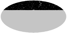
(a) High latitude, north hat with $b\geq 30^{\circ}$ (24.11%)

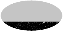
(b) High latitude, south hat with $b\leq-30^{\circ}$ (23.98%)

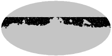
(c) Low latitude, north region with $0^{\circ}<b<30^{\circ}$ (15.15%)

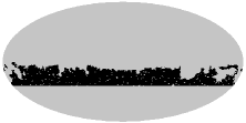
(d) Low latitude, south region with $-30^{\circ}<b<0^{\circ}$ (15.03%)

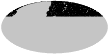
(e) North hat with high instrument noise (15.20%)

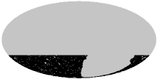
(f) South hat with high instrument noise (15.14%)

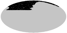
(g) North hat with low instrument noise (13.05%)

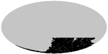
(h) South hat with low instrument noise (13.01%)

Fig. 3.—: Mask maps of various local areas defined by applying the Galactic latitude cuts [($a$)–($d$)] and the thresholds on the (smoothed) map of number-of-observations [($e$)–($h$)] on the KQ85 mask map. The black area corresponds to $M(p)=1$ while the grey area to $M(p)=0$. Each number in the parenthesis indicates the fraction of sky area with $M(p)=1$.

The left panel of Fig. 2 shows the angular power spectra of the WMAP 7-year temperature maps measured with the uniform (red) and the inverse-noise (blue dots with error bars) weighting schemes. We have used the sky area defined by the KQ85 mask that was adopted in the WMAP team’s temperature analysis. For a comparison, the WMAP team’s measurement has been shown together as grey dots with error bars (Larson et al. 2011). Our estimations of the angular power spectrum in both the uniform and the inverse-noise weighting schemes are consistent with the WMAP team’s estimation. We note that the amplitude of the power spectrum at the 41th bin ($851\leq l\leq 900$) is slightly larger than the WMAP team’s estimation, but they are statistically consistent with each other. Although statistically consistent, our result is a bit different from the WMAP team result at low $l$ region because the WMAP team applied the different estimation method (Blackwell-Rao estimator based on Gibbs sampling) at this low $l$ region while we simply used the pseudo power spectrum estimation method over the whole $l$ range.

The right panel of Fig. 2 shows the averaged angular power spectra measured from the 1000 mock data sets that mimic the WMAP instrument performance based on the concordance $\Lambda\textrm{CDM}$ model. The averaged power spectra based on both the uniform and the inverse-noise weighting schemes coincide with each other and restore the assumed model power spectrum (green curve) within measurement uncertainties, which demonstrates that our measuring algorithm works correctly. However, our algorithm gives a slightly positive bias with respect to the true value at the last two bins at the highest multipoles, where the uncertainty due to the finite size of the pixels is significantly large. Comparing the results based on the two weighting schemes, we can see that in a case of the inverse-noise weight scheme the size of error bars is bigger (smaller) at lower (higher) multipoles.

4 Power spectra of various local areas on the sky

Here we present the angular power spectra measured on various local regions on the sky defined based on the simple criteria such as the Galactic latitude or the number-of-observations cuts. To define a partial sky region, we basically use the KQ85 mask map and the number of observations at the W band (W4 DA). By putting a limit on the Galactic latitude or the number of observations, we have obtained several local regions with different characters.

Figure 3 summarizes the mask maps (or the window functions in the uniform weighting scheme) that are used in our power spectrum measurements. We estimate the angular power spectra on each local area using the corresponding mask map as a window function. Especially, the north hat ($b\geq 30^{\circ}$; $b$ is the Galactic latitude) and the south hat ($b\leq-30^{\circ}$) regions defined by the simple Galactic latitude cut show a difference in the power amplitude around the third peak of the angular power spectrum, which can be interpreted as the anomaly effect (see Fig. 4 below). To assess the statistical significance of the observed anomaly, we compare the difference of power spectrum amplitudes with the prediction of the fiducial flat $\Lambda\textrm{CDM}$ model. Then, we search for the origin of the observed anomaly by considering possibilities due to the residual Galaxy contamination, the WMAP instrument noise, and unresolved point sources.

4.1 North hat and south hat

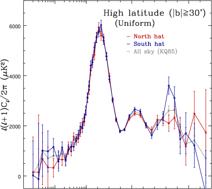
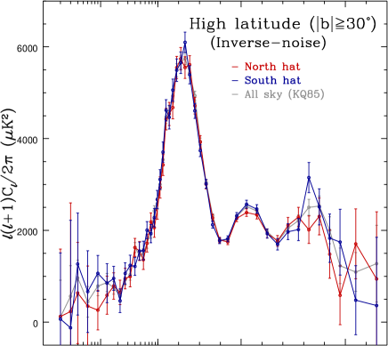
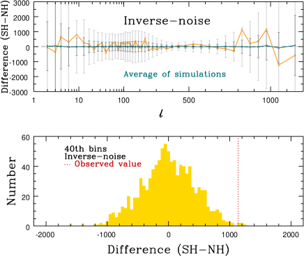
Fig. 4.—: (Top) Angular power spectra measured on the north hat and the south hat regions based on the uniform (left) and the inverse-noise (right panel) weighting schemes. The power spectra measured on the north hat ($b\geq 30^{\circ}$) are shown as red color while those on the south hat ($b\leq-30^{\circ}$) as blue color. The grey color denotes the result measured on the whole sky enclosed by KQ85 mask map. (Middle) Difference of powers between the south hat (SH) and north hat (NH) are shown (orange color). The averaged difference estimated from the one thousand WMAP mock data sets are shown as dark green dots with $1\sigma$ (dark grey) and $3\sigma$ (light grey) error bars. (Bottom) Histograms of differences between SH and NH powers in the 40th bin that corresponds to $801\leq l\leq 850$, measured from the $\Lambda\textrm{CDM}$ based WMAP mock data sets, for uniform (left) and inverse-noise (right panel) weighting schemes. The vertical red dashed lines indicate the difference values measured from the WMAP 7-year data.

Figure 4 displays the angular power spectra measured on the north hat and the south hat regions. Each power spectrum has been estimated in both the uniform and the inverse-noise weighting schemes separately. The overall features in the measured angular power spectra are similar to the power spectrum measured on the whole sky region with KQ85 mask (grey curves). However, the amplitudes of the power spectrum around the third peak show opposite deviations in the south hat and the north hat.

We can see such a difference more dramatically in the middle panels of Fig. 4, where the difference of powers between the south hat (SH) and north hat (NH) are displayed for an ease of comparison. We have also estimated the average and the variance of differences between SH and NH powers from the one thousand WMAP mock data sets, which are shown as dark green dots with $1\sigma$ (dark grey) and $3\sigma$ (light grey) error bars. Since we have assumed the homogeneity and isotropy of the universe during the production of the WMAP mock data sets, the average of differences is expected to be zero over the whole $l$ range. We note that in the third peak (that corresponds to the 40th bin; $801\leq l\leq 850$) the difference between SH and NH regions is statistically significant because it is located around the $3\sigma$ deviating from the zero value. The histogram of differences between SH and NH powers in the 40th bin measured from the $\Lambda\textrm{CDM}$ based WMAP mock data sets and the value measured from the WMAP data (vertical red dashed line) also confirms this result (bottom panels of Fig. 4).

4.2 Low latitude area

The foreground contamination at high Galactic latitude regions like the north hat and the south hat is generally expected to be small. Although the foreground model has been subtracted from the observed temperature fluctuations and the sky region that are significantly contaminated by the Galactic emission has been excluded by the KQ85 mask, we can expect that the residual foreground emission at low latitude regions may be stronger than high latitude regions such as the north hat and the south hat. We estimated angular power spectra on two separate regions at the low Galactic latitude defined as low latitude north ($0^{\circ}<b<30^{\circ}$) and south ($-30^{\circ}<b<0^{\circ}$) regions, where the Galactic plane region has been excluded by the KQ85 mask. The results are presented in Fig. 5 with a similar format as in Fig. 4.

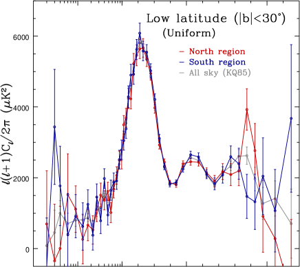
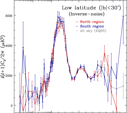
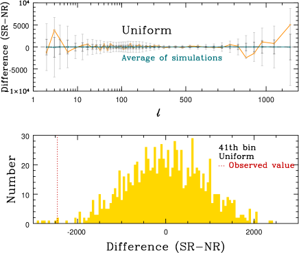
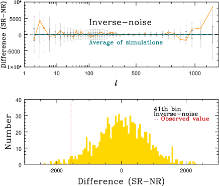
Fig. 5.—: Similar to Fig. 4, but for regions at the low Galactic latitude areas ($|b|<30^{\circ}$). The power spectra are measured on the north region (NR; $0^{\circ}<b<30^{\circ}$; red color) and on the south region (SR; $-30^{\circ}<b<0^{\circ}$; blue color). In the bottom panels, shown are histograms of power differences at the 41th $l$-bin ($851\leq l\leq 900$) between south and north regions, expected in the concordance $\Lambda\textrm{CDM}$ model, together with observed values from the WMAP 7-year data (vertical red dashed lines).

The angular power spectra measured on the sky regions that are expected to be contaminated by the residual Galactic foreground emission show different features from those seen in the cases of the north and south hats. The behavior of power spectrum amplitudes around the third peak is opposite to the case of north versus south hat regions. The power on the low latitude north region is larger than that on the south region, and the difference between the north and the south regions is more significant at the 41th bin ($851\leq l\leq 900$). The difference is again statistically significant with a $3\sigma$ deviation from the zero value (for uniform weighting scheme), which is another anomaly found in this work. Although not shown here, if we consider the whole northern and southern hemispheres as two localized regions, then the anomalies at high and low Galactic latitudes are compensated and not noticeable. Furthermore, there are two more noticeable differences between the north and the south regions at the second bin ($l=3$) and at the last bin ($1101\leq l\leq 1200$). For the latter, the measured difference exceeds $3\sigma$ from the zero value for the inverse-noise weighting scheme (see also Table 1 below). Therefore, based on this comparison, it seems that the north-south anomaly around the third peak of the angular power spectrum observed on the high Galactic latitude north and south hat regions is not due to any possible residual Galactic foreground emission.

4.3 Instrument noise

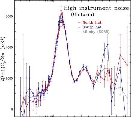
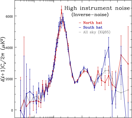
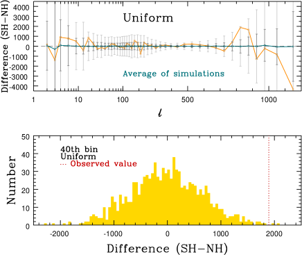
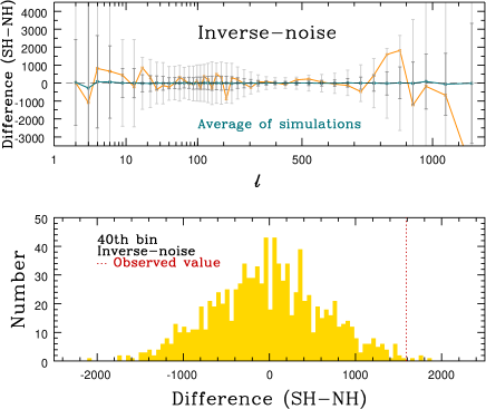
Fig. 6.—: Similar to Fig. 4, but for regions with high instrument noise ($N_{\textrm{\scriptsize obs}}<2500$ on the number-of-observations map at W4 DA smoothed with $\textrm{FWHM}=1^{\circ}$) that belong to the north hat (left) and the south hat (right).

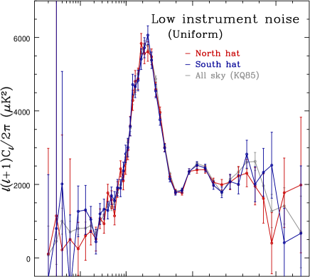
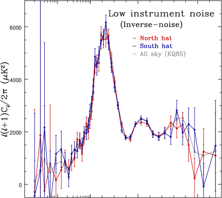
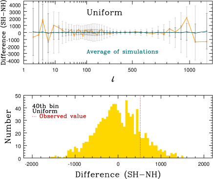
Fig. 7.—: Similar to Fig. 4, but for regions with the low instrument noise ($N_{\textrm{\scriptsize obs}}>2035$) belonging to the north hat (left) and the south hat (right).

Although the WMAP satellite probed the CMB temperature fluctuations on the whole sky, its scanning strategy is somewhat inhomogeneous such that the regions near the ecliptic poles were probed many times as compared to the regions near the ecliptic plane. Thus, it is expected that the CMB anisotropy is strongly affected by the instrument noise in the ecliptic plane region. To quantify such an effect due to the WMAP instrument noise, we use the number of observations, $N_{\textrm{\scriptsize obs}}(p)$, at the WMAP W4 frequency channel, which is shown in Fig. 1.

Defining regions with high and low instrument noise by simply putting threshold limits on the number of observations results in the geometrical sky regions whose boundary is not smooth and the pixels near the boundary are not contiguous with many small islands outside the primary region, which prevents us to obtain the unbiased estimation of the power spectrum. To avoid this problem, we have used the Smoothing program of the HEALPix software to smooth the map of number-of-observations at the W4 frequency channel with a Gaussian filter of $1^{\circ}$ FWHM. Then, we define the north hat (or the south hat) regions with high instrument noise by selecting pixels with $N_{\textrm{\scriptsize obs}}(p)<2500$ on the smoothed number-of-observations map. We also exclude the island areas that are not included in the primary big regions. Similarly, to define the regions with low instrument noise, we set $N_{\textrm{\scriptsize obs}}(p)>2035$ on the same map. The threshold value for the number of observations at the region of high (low) instrument noise has been set to obtain the sky area of about 15% (13%) of the whole sky for $N_{\textrm{\scriptsize obs}}(p)<2500$ ($N_{\textrm{\scriptsize obs}}(p)>2035$). For ecliptic plane regions with high instrument noise (i.e., with low number of observations), we choose the threshold value to include the larger sky area for the purpose of reducing the statistical variance in the power spectrum measurement. The sky regions defined in this way are shown in Fig. 3 $(e)$–$(h)$.

We have measured angular power spectra on the ecliptic plane regions with small number of observations (defined as $N_{\textrm{\scriptsize obs}}<2500$) that belong to the north hat or the south hat regions. The results are shown in Fig. 6. The angular power spectra measured on the ecliptic plane regions (that belong to the north hat or the south hat regions) show the behavior that is similar to the case of the whole north hat and south hat regions (see Fig. 4). The difference of power spectrum amplitudes between the south and the north hats still statistically significant, deviating from the zero value up to $3\sigma$.

Table 1. : Probabilities of finding the north-south (absolute) difference larger than the observed value, estimated based on one thousand $\Lambda\textrm{CDM}$ based WMAP mock data sets. The $l_{b}$ and $\Delta l$ denote the multipole $l$ value at the center of the bin and the bin-width, respectively, used in the power spectrum estimation.

				$p$ value (%)
area	bin number	$l_{b}$	$\Delta l$
				uniform weighting	inverse-noise weighting
High Galactic latitude ($|b|\geq 30^{\circ}$)	40	825	50	$0.1$	$0.7$
—with high instrument noise	40	825	50	$0.5$	$1.0$
—with low instrument noise	40	825	50	$31$	$19$
—with 20% increased bin-width	39	825	60	$0.0$	$0.8$
—with 50% increased bin-width	39	825	75	$0.0$	$2.5$
High Galactic latitude ($|b|\geq 25^{\circ}$)	40	825	50	$0.6$	$5.9$
High Galactic latitude ($|b|\geq 35^{\circ}$)	40	825	50	$0.0$	$0.0$
High Galactic latitude ($|b|\geq 40^{\circ}$)	40	825	50	$1.5$	$1.1$
High Galactic latitude ($|b|\geq 45^{\circ}$)	40	825	50	$20$	$12$
Low Galactic latitude ($|b|<30^{\circ}$)	41	875	50	$0.5$	$5.0$
	45	1150	100	$8.5$	$0.1$

We have also measured angular power spectra on the ecliptic pole regions with large number of observations (defined as $N_{\textrm{\scriptsize obs}}(p)>2035$), which are shown in Fig. 7. Here, the power spectra measured on the ecliptic pole regions in the north hat and the south hat are consistent with each other in the $l$ range around the third peak. They are also very consistent with the power spectrum measured on the whole sky with KQ85 mask (grey dots with error bars). Around the third peak, the power spectrum measured on the ecliptic pole regions in the north hat is very similar to the case of the whole north hat region, while the power spectrum measured on the ecliptic pole regions in the south hat has decreased in amplitude compared with the case of the whole south hat region (see Fig. 4). As a result, the observed north-south difference in the 40th bin of the power spectrum is around $1\sigma$ confidence limit and is not statistically significant any more (bottom panels of Fig. 7). These results strongly suggest that the north-south anomaly around the third peak likely originates from the unknown systematic effects contained on the sky regions that are affected by strong instrument noise.

Based on the one thousand WMAP mock data sets, we count the number of cases where the magnitude of the north-south power difference is larger than the observed value for several chosen local regions. The results are summarized in Table 1 for particular $l$-bins where the high statistical significance is seen. The listed $p$-values are probabilities of finding the north-south (absolute) difference larger than the observed value. Although the statistical significance for the north-south anomaly at the high latitude regions becomes weaker for the inverse-noise weighting scheme, the observed anomaly is still rare in the $\Lambda\textrm{CDM}$ universe with $p=0.7$%. Comparing the cases for high and low instrument noise at the high latitude regions strongly suggests that the north-south anomaly around the third peak come from the region dominated by the WMAP instrument noise.

4.4 Point sources

Recently, the Planck point source catalogue has been publicly available (Planck Collaboration 2011b). We take the Planck Early Release Compact Source Catalogue (ERCSC) at 100 GHz frequency band and exclude the sources at high Galactic latitude ($|b|\geq 30^{\circ}$) whose angular position on the sky is located at the excluded region with $M(p)=0$ in the KQ85 mask map. The remaining 163 radio point sources at $|b|\geq 30^{\circ}$ are considered as the sources that were newly discovered by the Planck satellite at 100 GHz. By excluding (i.e., by assigning $M(p)=0$ at) the circular areas centered on these point sources with radius $0\hbox{$.\!\!^{\circ}$}6$ in the WMAP team’s KQ85 mask map, we have produced a new mask map (or window function) and measured the angular power spectra based on this new window function. Because the number of newly discovered sources are very small, the additional exclusion of point sources almost does not affect the angular power spectra on the north and the south hat regions. Therefore, at the present stage we cannot find any evidence that the north-south anomaly around the third peak of the angular power spectrum originates from the unresolved point sources.

4.5 Dependence of the north-south anomaly on the bin-width and the Galactic latitude cut

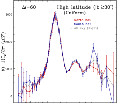
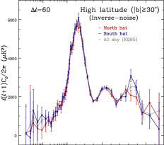
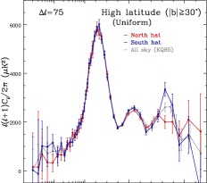
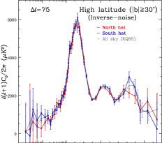
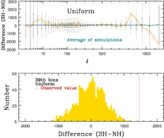
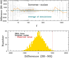
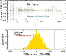
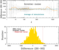
Fig. 8.—: Similar to Fig. 4 but now the bin-width has been increased by a factor of $1.2$ (first two panels) and $1.5$ (last two panels). The 39th bin centered at $l=825$ corresponds to our focused bin located around at the third peak with the bin ranging over $796\leq l\leq 855$ ($\Delta l=60$) for 20% increased bin-width and $788\leq\ell\leq 862$ ($\Delta l=75$) for 50% increased one. The results obtained in the uniform weighting scheme are shown on the first and the third panels while those in the inverse-noise weighting scheme on the second and the fourth ones. In both cases, the high Galactic latitude regions with $|b|\geq 30^{\circ}$ have been used. For the power spectrum measured on the whole sky enclosed by KQ85 mask (denoted as grey color), the original $l$-binning has been used as in Fig. 4.

Here we investigate the effect of the bin-width and the Galactic latitude cut on the detected north-south anomaly around the third peak in the angular power spectrum measured from the WMAP 7-year data.

Our detection of the north-south anomaly is based on the 40th bin around the third peak which ranges over $851\leq l\leq 900$ ($\Delta l=50$); see Fig. 4. By fixing the bin center at $l=825$, we have increased the bin-width by 20% ($796\leq l\leq 855$; $\Delta l=60$) and 50% ($788\leq l\leq 862$; $\Delta l=75$). During the re-binning process, we reduce the total number of bins into 43 and widen the width of adjacent bins appropriately; now our focused bin centered at $l=825$ is located at the 39th bin. Based on the new $l$-binning, we have measured angular power spectra from the WMAP 7-year data and one thousand sets of WMAP mock observations. The results are shown in Fig. 8. In the case of the uniform weighting scheme, the increase of the bin-width increases the statistical significance of the north-south anomaly; there is no occurrence of such an anomaly larger than the observed one among the one thousand WMAP simulations. However, in the case of the inverse-noise weighting scheme, the statistical significance slightly decreases for the 50% increased bin-width (see Table 1 for the summary of statistical significances).

We also look into how our conclusion is sensitive to the Galactic latitude cut. We compare the power spectrum measurements for different latitude cuts, $|b|=25^{\circ}$, $30^{\circ}$, $35^{\circ}$, $40^{\circ}$, and $45^{\circ}$ (Fig. 9; the case of $|b|=30^{\circ}$ is presented in Fig. 4). We notice that the north-south anomaly becomes the most significant in the case of $|b|=35^{\circ}$ cut, and no such an anomaly occurs in both weighting schemes among the one thousand WMAP mock data sets (see Table 1). Furthermore, the statistical significance of this anomaly becomes weaker as the latitude cut higher or lower than $|b|=35^{\circ}$ is applied. For $|b|=25^{\circ}$ ($45^{\circ}$), the $p$ value is $5.9$% ($12$%) in the inverse-noise weighting scheme. Up to the Galactic latitude cut $|b|=40^{\circ}$, the north-south anomaly is maintained with a high statistical significance (see Table 1). For higher latitude cuts like $|b|\geq 45^{\circ}$, however, the north-south anomaly in the power spectrum amplitude does not have the statistical significance any more.

According to the two results shown above, the observed north-south anomaly has weak dependences on the bin-width used in the power spectrum estimation and the Galactic latitude cut, which implies that the north-south anomaly is the realistic feature present in the WMAP data and supports our primary conclusion.

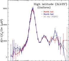
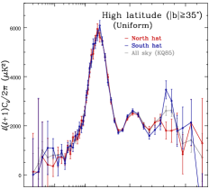
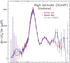
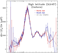
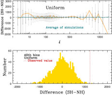
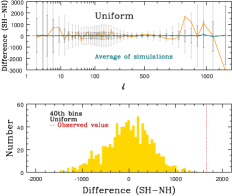
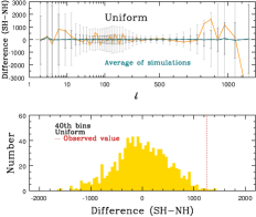
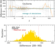
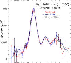
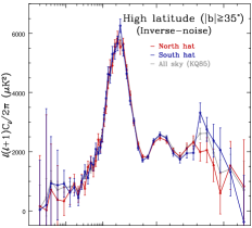
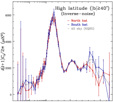
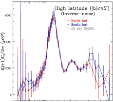
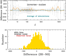
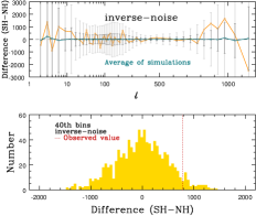
Fig. 9.—: Angular power spectra measured on the north and the south hat regions defined by different Galactic latitude cuts (from left to right, $|b|=25^{\circ}$, $35^{\circ}$, $40^{\circ}$, $45^{\circ}$), with a similar format given in Fig. 4 (the case of $|b|=30^{\circ}$). Fractions of the sky area for north (south) regions are 27.7% (27.6%), 20.6% (20.5%), 17.2% (17.3%), 14.1% (14.2%), respectively, in increasing order of the latitude cut. Top panels are for the uniform weighting scheme while bottom panels for the inverse-noise weighting scheme.

5 Conclusions

In this work we have compared the angular power spectra measured on various local sky regions using the WMAP 7-year temperature anisotropy data. The sky regions studied in this work are the low Galactic contamination regions at high Galactic latitude (north hat and south hat), the strong Galactic contamination regions at low Galactic latitude north and south regions, the regions dominated by the WMAP instrument noise (ecliptic plane regions), and the regions of low instrument noise (ecliptic pole regions).

We found that the power spectra around the third peak measured on the north hat and the south hat regions show an anomaly which is statistically significant, deviating around $3\sigma$ from the $\Lambda\textrm{CDM}$ model prediction. We have tried to identify the cause of this anomaly by performing the similar analysis on the low latitude regions and the regions with high or low instrument noise. Curiously, in the low Galactic latitude ($|b|<30^{\circ}$) there appears another but less statistically significant north-south anomaly around the third peak, whose behavior is opposite to the one seen in the high latitude regions and compensates the anomalies in the whole northern and southern hemispheres. At the present situation, we cannot draw any firm conclusion for the origin of the observed anomaly. However, we found that the observed north-south anomaly maintains with the high statistical significance in the power spectra measured on the regions with high instrument noise, and the anomaly becomes weaker in the power spectra on the regions with low instrument noise. Thus, in our present analysis the observed anomaly is significant on the sky regions that are dominated by the WMAP instrument noise. We have verified that the observed north-south anomaly around the third peak has only weak dependences on the bin-width used in the power spectrum estimation and the Galactic latitude cut, which strengthens our conclusion (see Figs. 8 and 9).

The location of the third peak in the angular power spectrum corresponds to the angular scale that approaches the WMAP resolution limit and that is dominated by the WMAP instrument noise. Because the Planck satellite probes the CMB anisotropy with higher angular resolution and sensitivity than the WMAP, we expect that the origin of the observed anomaly will be identified in more detail when the Planck data becomes publicly available (Planck Collaboration et al. 2011a).

It is possible that our detection of the north-south anomaly may be strongly driven by a posteriori statistics based on the fact that we have computed the power spectra on two different parts of the sky and only then noticed a peculiar discrepancy between the two power amplitudes in one bin around the third peak, neglecting the fact that there could have been a similar discrepancy at any of the other multipole bins (see Zhang & Huterer 2010 for the related discussion). One may argue that we may properly quantify the statistical significance of the detected anomaly from the distribution of maximum north-south differences (in unit of standard deviation) over all multipole bins. The result for north and south hats ($|b|\geq 30^{\circ}$) in the uniform weighting scheme is shown in Fig. 10. In the histogram of one thousand values of the maximum (among 45 bins) north-south power difference in unit of standard deviation, each estimated from the WMAP mock observations, the detected north-south anomaly around the third peak becomes statistically less significant; the probability of finding cases with a deviation larger than the measured value is $p=75/1000=7.5$% which is slightly less than $2\sigma$ confidence limit.

However, it should be emphasized that the point described above is correct only under the condition that the power spectrum at different multipoles is equally affected by exactly the same CMB physics, Galaxy foreground, and instrument noise properties, which is generally not true in our case of harmonic space. The power spectrum at low multipoles is dominated by the integrated Sachs-Wolfe effect and is more affected by the survey geometry while the power spectrum at higher multipoles is more concerned with the physics of acoustic oscillation and the WMAP instrument noise. For example, it is not justified to consider all multipole bins in quantifying the statistical significance of an anomaly detected in one multipole bin if the anomaly originates from the phenomenon that is influential at the local multipole range. Therefore, our original interpretation of the detected north-south anomaly around the third peak as statistically significant based on the analysis focusing on the corresponding multipole bin is still valid before the origin of the anomaly becomes unveiled.

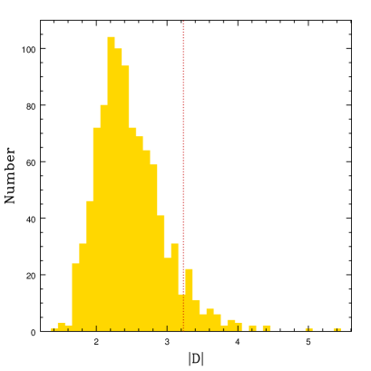
Fig. 10.—: A histogram of one thousand values of the maximum (among 45 bins) north-south power difference in unit of standard deviation, $|D|=\textrm{Max}(|C_{b}^{\textrm{\tiny NH}}-C_{b}^{\textrm{\tiny SH}}|/\sigma_{b})$, where $C_{b}^{\textrm{\tiny NH}}$ ($C_{b}^{\textrm{\tiny SH}}$) is the $b$-th band power measured at the north (south) hat region ($|b|\geq 30^{\circ}$), and $\sigma_{b}$ is the standard deviation of the power difference at the $b$-th multipole bin estimated from the WMAP simulation data sets, equivalent to the size of dark grey ($1\sigma$) error bars in the middle-left panel of Fig. 4. The vertical red dashed line indicates the measured value with $|D|=3.23$.

As the Planck data will be soon available, we anticipate that our issue of whether the anomaly is intrinsic one or due to the WMAP instrument noise will be resolved by the Planck data.

ACKNOWLEDGMENTS We acknowledge the use of the Legacy Archive for Microwave Background Data Analysis (LAMBDA). Support for LAMBDA is provided by the NASA Office of Space Science. Some of the results in this paper have been derived using the HEALPix and the CAMB softwares. This work was supported by the Korea Research Foundation Grant funded by the Korean Government (KRF-2008-341-C00022).

References

- Alpher & Herman (1948) Alpher, R.A. & Herman, R. 1948, Evolution of the Universe, Nature, 162, 774
- Ansari et al. (2010) Ansari, R. & Magneville, C. 2010, Partial CMB maps: bias removal and optimal binning of the angular power spectrum, MNRAS, 405, 1421
- Basak & Delabrouille (2012) Basak, S. & Delabrouille, J. 2012, A needlet internal linear combination analysis of WMAP 7-year data: estimation of CMB temperature map and power spectrum, MNRAS, 419, 1163
- Benoît et al. (2003) Benoît, A., Ade, P., Amblard, A., et al. 2003, The cosmic microwave background anisotropy power spectrum measured by Archeops, A&A, 399, L19
- Bennett et al. (2003) Bennett, C.L., Halpern, M., Hinshaw, G., et al. 2003, First-Year Wilkinson Microwave Anisotropy Probe (WMAP) Observations: Preliminary Maps and Basic Results, ApJS, 148, 1
- Bernui (2008) Bernui, A. 2008, Anomalous CMB north-south asymmetry, Phys. Rev. D, 78, 063531
- Bond & Efstathiou (1987) Bond, J.R. & Efstathiou, G. 1987, The statistics of cosmic background radiation fluctuations, MNRAS, 226, 655
- Bond et al. (1998) Bond, J.R., Jaffe, A.H., & Knox, L. 1998, Estimating the power spectrum of the cosmic microwave background, Phys. Rev. D, 57, 2117
- Brown et al. (2005) Brown, M.L., Castro, P.G., & Taylor, A.N. 2005, Cosmic microwave background temperature and polarization pseudo- estimators and covariances, MNRAS, 360, 1262
- Brown et al. (2009) Brown, M.L., Ade, P., Bock, J., et al. 2009, Improved Measurements of the Temperature and Polarization of the Cosmic Microwave Background from QUaD, ApJ, 705, 978
- Carlstrom et al. (2003) Carlstrom, J.E., Kovac, J., Leitch, E.M., & Pryke, C. 2003, Status of CMB polarization measurements from DASI and other experiments, New Astron. Rev., 47, 953
- Chiang & Chen (2012) Chiang, L.Y. & Chen, F.F. 2012, Direct Measurement of the Angular Power Spectrum of Cosmic Microwave Background Temperature Anisotropies in the WMAP Data, ApJ, 751, 43
- Chon et al. (2004) Chon, G., Challinor, A., Prunet, S., Hivon, E., & Szapudi, I. 2004, Fast estimation of polarization power spectra using correlation functions, MNRAS, 350, 914
- Dahlen & Simons (2008) Dahlen, F.A., & Simons, F.J. 2008, Spectral estimation on a sphere in geophysics and cosmology, Geophysical Journal International, 174, 774
- Das et al. (2009) Das, S., Hajian, A., & Spergel, D.N. 2009, Efficient power spectrum estimation for high resolution CMB maps, Phys. Rev. D, 79, 083008
- Dicke et al. (1965) Dicke, R.H., Peebles, P.J.E., Roll, P.G., & Wilkinson, D.T. 1965, Cosmic Black-Body Radiation, ApJ, 142, 414
- Efstathiou (2004) Efstathiou, G. 2004, Myths and truths concerning estimation of power spectra: the case for a hybrid estimator, MNRAS, 349, 603
- Eriksen et al. (2004a) Eriksen, H.K., O’Dwyer, I.J., Jewell, J.B., et al. 2004a, Power Spectrum Estimation from High-Resolution Maps by Gibbs Sampling, ApJS, 155, 227
- Eriksen et al. (2004b) Eriksen, H.K., Hansen, F.K., Banday, A.J., Górski, K.M., & Lilje, P.B. 2004b, Asymmetries in the Cosmic Microwave Background Anisotropy Field, ApJ, 605, 14
- Eriksen et al. (2004c) Eriksen, H.K., Novikov, D.I., Lilje, P.B., Banday, A.J., & Górski, K.M. 2004c, Testing for Non-Gaussianity in the Wilkinson Microwave Anisotropy Probe Data: Minkowski Functionals and the Length of the Skeleton, ApJ, 612, 64
- Eriksen et al. (2007a) Eriksen, H.K., Huey, G., Saha, R., et al. 2007a, A Reanalysis of the 3 Year Wilkinson Microwave Anisotropy Probe Temperature Power Spectrum and Likelihood, ApJ, 656, 641
- Eriksen et al. (2007b) Eriksen, H.K., Banday, A.J., Górski, K.M., Hansen, F.K., & Lilje, P.B. 2007b, Hemispherical Power Asymmetry in the Third-Year Wilkinson Microwave Anisotropy Probe Sky Maps, ApJ, 660, L81
- Fay et al. (2008) Faÿ, G., Guilloux, F., Betoule, M., et al. 2008, CMB power spectrum estimation using wavelets, Phys. Rev. D, 78, 083013
- Fowler et al. (2010) Fowler, J.W., Acquaviva, V., Ade, P.A.R., et al. 2010, The Atacama Cosmology Telescope: A Measurement of the Cosmic Microwave Background Power Spectrum at 148 GHz, ApJ, 722, 1148
- Górski (1994) Górski, K. M. 1994, ApJ, On determining the spectrum of primordial inhomogeneity from the COBE DMR sky maps: Method, 430, L85
- Górski et al. (1999) Górski, K.M., Wandelt, B.D., Hansen, F.K., Hivon, E., & Banday, A.J. 1999, The HEALPix Primer, arXiv:astro-ph/9905275
- Górski et al. (2005) Górski, K.M., Hivon, E., Banday, A.J., et al. 2005, HEALPix: A Framework for High-Resolution Discretization and Fast Analysis of Data Distributed on the Sphere, ApJ, 622, 759
- Hansen et al. (2002) Hansen, F.K., Górski, K.M., & Hivon, E. 2002, Gabor transforms on the sphere with applications to CMB power spectrum estimation, MNRAS, 336, 1304
- Hansen et al. (2004a) Hansen, F.K., Banday, A.J., & Górski, K.M. 2004a, Testing the cosmological principle of isotropy: local power-spectrum estimates of the WMAP data, MNRAS, 354, 641
- Hansen et al. (2004b) Hansen, F.K., Balbi, A., Banday, A.J., & Górski, K.M. 2004b, Cosmological parameters and the WMAP data revisited, MNRAS, 354, 905
- Hansen et al. (2009) Hansen, F.K., Banday, A.J., Górski, K.M., Eriksen, H.K., & Lilje, P.B. 2009, Power Asymmetry in Cosmic Microwave Background Fluctuations from Full Sky to Sub-Degree Scales: Is the Universe Isotropic?, ApJ, 704, 1448
- Hinshaw et al. (2003) Hinshaw, G., Spergel, D.N., Verde, L., et al. 2003, First-Year Wilkinson Microwave Anisotropy Probe (WMAP) Observations: The Angular Power Spectrum, ApJS, 148, 135
- Hinshaw et al. (2007) Hinshaw, G., Nolta, M.R., Bennett, C.L., et al. 2007, Three-Year Wilkinson Microwave Anisotropy Probe (WMAP) Observations: Temperature Analysis, ApJS, 170, 288
- Hivon et al. (2002) Hivon, E., Górski, K.M., Netterfield, C.B., et al. 2002, MASTER of the Cosmic Microwave Background Anisotropy Power Spectrum: A Fast Method for Statistical Analysis of Large and Complex Cosmic Microwave Background Data Sets, ApJ, 567, 2
- Hoftuft et al. (2009) Hoftuft, J., Eriksen, H.K., Banday, A.J., et al. 2009, Increasing Evidence for Hemispherical Power Asymmetry in the Five-Year WMAP Data, ApJ, 699, 985
- Hu & Dodelson (2002) Hu, W. & Dodelson, S. 2002, Cosmic Microwave Background Anisotropies, ARA&A, 40, 171
- Huffenberger et al. (2006) Huffenberger, K.M., Eriksen, H.K., & Hansen, F.K. 2006, Point-Source Power in 3 Year Wilkinson Microwave Anisotropy Probe Data, ApJ, 651, L81
- Jarosik et al. (2011) Jarosik, N., Bennett, C.L., Dunkley, J., et al. 2011, Seven-year Wilkinson Microwave Anisotropy Probe (WMAP) Observations: Sky Maps, Systematic Errors, and Basic Results, ApJS, 192, 14
- Jones et al. (2006) Jones, W.C., Ade, P.A.R., Bock, J.J., et al. 2006, A Measurement of the Angular Power Spectrum of the CMB Temperature Anisotropy from the 2003 Flight of BOOMERANG, ApJ, 647, 823
- Keisler et al. (2011) Keisler, R., Reichardt, C.L., Aird, K.A., et al. 2011, A Measurement of the Damping Tail of the Cosmic Microwave Background Power Spectrum with the South Pole Telescope, ApJ, 743, 28
- Komatsu et al. (2009) Komatsu, E., Dunkley, J., Nolta, M.R., et al. 2009, Five-Year Wilkinson Microwave Anisotropy Probe Observations: Cosmological Interpretation, ApJS, 180, 330
- Komatsu et al. (2011) Komatsu, E., Smith, K.M., Dunkley, J., et al. 2011, Seven-year Wilkinson Microwave Anisotropy Probe (WMAP) Observations: Cosmological Interpretation, ApJS, 192, 18
- Larson et al. (2011) Larson, D., Dunkley, J., Hinshaw, G., et al. 2011, Seven-year Wilkinson Microwave Anisotropy Probe (WMAP) Observations: Power Spectra and WMAP-derived Parameters, ApJS, 192, 16
- Lee et al. (2001) Lee, A.T., Ade, P., Balbi, A., et al. 2001, A High Spatial Resolution Analysis of the MAXIMA-1 Cosmic Microwave Background Anisotropy Data, ApJ, 561, L1
- Lewis et al. (2000) Lewis, A., Challinor, A., & Lasenby, A. 2000, Efficient Computation of Cosmic Microwave Background Anisotropies in Closed Friedmann-Robertson-Walker Models, ApJ, 538, 473
- Mason et al. (2003) Mason, B.S., Pearson, T.J., Readhead, A.C.S., et al. 2003, The Anisotropy of the Microwave Background to : Deep Field Observations with the Cosmic Background Imager, ApJ, 591, 540
- Mitra et al. (2009) Mitra, S., Sengupta, A.S., Ray, S., Saha, R., & Souradeep, T. 2009, Cosmic microwave background power spectrum estimation with non-circular beam and incomplete sky coverage, MNRAS, 394, 1419
- Mortlock et al. (2002) Mortlock, D.J., Challinor, A.D., & Hobson, M.P. 2002, Analysis of cosmic microwave background data on an incomplete sky, MNRAS, 330, 405
- Nolta et al. (2009) Nolta, M.R., Dunkley, J., Hill, R.S., et al. 2009, Five-Year Wilkinson Microwave Anisotropy Probe Observations: Angular Power Spectra, ApJS, 180, 296
- Oh et al. (1999) Oh, S.P., Spergel, D.N., & Hinshaw, G. 1999, An Efficient Technique to Determine the Power Spectrum from Cosmic Microwave Background Sky Maps, ApJ, 510, 551
- Page et al. (2003) Page, L., Nolta, M.R., Barnes, C., et al. 2003, First-Year Wilkinson Microwave Anisotropy Probe (WMAP) Observations: Interpretation of the TT and TE Angular Power Spectrum Peaks, ApJS, 148, 233
- Page et al. (2007) Page, L., Hinshaw, G., Komatsu, E., et al. 2007, Three-Year Wilkinson Microwave Anisotropy Probe (WMAP) Observations: Polarization Analysis, ApJS, 170, 335
- Park (2004) Park, C.-G. 2004, Non-Gaussian signatures in the temperature fluctuation observed by the Wilkinson Microwave Anisotropy Probe, MNRAS, 349, 313
- Peebles & Yu (1970) Peebles, P.J.E. & J.T. Yu, J.T. 1970, Primeval Adiabatic Perturbation in an Expanding Universe, ApJ, 162, 815
- Peiris et al. (2003) Peiris, H.V., Komatsu, E., Verde, L., et al. 2003, First-Year Wilkinson Microwave Anisotropy Probe (WMAP) Observations: Implications For Inflation, ApJS, 148, 213
- Penzias & Wilson (1965) Penzias A.A. & Wilson R.W. 1965, A Measurement of Excess Antenna Temperature at 4080 Mc/s, ApJ, 142, 419
- Planck Collaboration et al. (2011a) Planck Collaboration, Ade, P.A.R., Aghanim, N., et al. 2011a, Planck early results. I. The Planck mission, A&A, 536, A1
- Planck Collaboration (2011b) Planck Collaboration, Ade, P.A.R., Aghanim, N., et al. 2011, Planck early results. VII. The Early Release Compact Source Catalogue, A&A, 536, A7
- Polenta et al. (2005) Polenta, G., Marinucci, D., Balbi, A., et al. 2005, Unbiased estimation of an angular power spectrum, J. Cosmol. Astropart. Phys., 11, 1
- Reichardt et al. (2009) Reichardt, C.L., Ade, P.A.R., Bock, J.J., et al. 2009, High-Resolution CMB Power Spectrum from the Complete ACBAR Data Set, ApJ, 694, 1200
- Sachs & Wolfe (1967) Sachs, R.K. & Wolfe, A.M. 1967, Perturbations of a Cosmological Model and Angular Variations of the Microwave Background, ApJ, 147, 73
- Saha et al. (2006) Saha, R., Jain, P., & Souradeep, T. 2006, A Blind Estimation of the Angular Power Spectrum of CMB Anisotropy from WMAP, ApJ, 645, L89
- Saha et al. (2008) Saha, R., Prunet, S., Jain, P., & Souradeep, T. 2008, CMB anisotropy power spectrum using linear combinations of WMAP maps, Phys. Rev. D, 78, 023003
- Samal et al. (2010) Samal, P.K., Saha, R., Delabrouille, J., et al. 2010, Cosmic Microwave Background Polarization and Temperature Power Spectra Estimation Using Linear Combination of WMAP 5 Year Maps, ApJ, 714, 840
- Scott & Smoot (2006) Scott, D. & Smoot, G. 2006, Cosmic Microwave Background Mini-Review, arXiv:astro-ph/0601307
- Smoot et al. (1992) Smoot, G.F., Bennett, C.L., Kogut, A., et al. 1992, Structure in the COBE differential microwave radiometer first-year maps, ApJ, 396, L1
- Souradeep et al. (2006) Souradeep, T., Saha, R., & Jain, P. 2006, Angular power spectrum of CMB anisotropy from WMAP, New Astron. Rev., 50, 854
- Spergel et al. (2003) Spergel, D.N., Verde, L., Peiris, H.V., et al. 2003, First-Year Wilkinson Microwave Anisotropy Probe (WMAP) Observations: Determination of Cosmological Parameters, ApJS, 148, 175
- Spergel et al. (2007) Spergel, D.N., Bean, R., Doré, O., et al. 2007, Three-Year Wilkinson Microwave Anisotropy Probe (WMAP) Observations: Implications for Cosmology, ApJS, 170, 377
- Szapudi et al. (2001) Szapudi, I., Prunet, S., Pogosyan, D., Szalay, A.S., & Bond, J.R. 2001, Fast Cosmic Microwave Background Analyses via Correlation Functions, ApJ, 548, L115
- Tegmark (1997) Tegmark, M. 1997, How to measure CMB power spectra without losing information, Phys. Rev. D, 55, 5895
- Wandelt et al. (2001) Wandelt, B.D., Hivon, E., & Górski, K.M. 2001, Cosmic microwave background anisotropy power spectrum statistics for high precision cosmology, Phys. Rev. D, 64, 083003
- Wandelt et al. (2003) Wandelt, B.D. & Hansen, F.K. 2003, Fast, exact CMB power spectrum estimation for a certain class of observational strategies, Phys. Rev. D, 67, 023001
- Wandelt et al. (2004) Wandelt, B.D., Larson, D.L., & Lakshminarayanan, A. 2004, Global, exact cosmic microwave background data analysis using Gibbs sampling, Phys. Rev. D, 70, 083511
- Yoho et al. (2011) Yoho, A., Ferrer, F., & Starkman, G.D. 2011, Degree-scale anomalies in the CMB: Localizing the first peak dip to a small patch of the north ecliptic sky, Phys. Rev. D, 83, 083525
- Zhang & Huterer (2010) Zhang, R., & Huterer, D. 2010, Disks in the sky: A reassessment of the WMAP“cold spot”?, Astroparticle Physics, 33, 69