MAGNETICALLY CONTROLLED ACCRETION FLOWS ONTO YOUNG STELLAR OBJECTS

Abstract

Accretion from disks onto young stars is thought to follow magnetic field lines from the inner disk edge to the stellar surface. The accretion flow thus depends on the geometry of the magnetic field. This paper extends previous work by constructing a collection of orthogonal coordinate systems, including the corresponding differential operators, where one coordinate traces the magnetic field lines. This formalism allows for an (essentially) analytic description of the geometry and the conditions required for the flow to pass through sonic points. Using this approach, we revisit the problem of magnetically controlled accretion flow in a dipole geometry, and then generalize the treatment to consider magnetic fields with multiple components, including dipole, octupole, and split monopole contributions. This approach can be generalized further to consider more complex magnetic field configurations. Observations indicate that accreting young stars have substantial dipole and octupole components, and that accretion flow is transonic. If the effective equation of state for the fluid is too stiff, however, the flow cannot pass smoothly through the sonic points in steady state. For a multipole field of order $\ell$, we derive a general constraint on the polytropic index, $n>\ell$ + 3/2, required for steady transonic flow to reach free-fall velocities. For octupole fields, inferred on surfaces of T Tauri stars, the index $n>9/2$, so that the flow must be close to isothermal. The inclusion of octupole field components produces higher densities at the stellar surface and smaller areas for the hot spots, which occur at higher latitudes; the magnetic truncation radius is smaller (larger) for octupole components that are aligned (anti-aligned) with the stellar dipole. This contribution thus increases our understanding of magnetically controlled accretion for young stellar objects and can be applied to a variety of additional astrophysical problems.

1 Introduction

During the star formation process, most of the mass that becomes part of the nascent star initially falls onto a surrounding circumstellar disk, rather than directly onto the stellar surface. This accretion process can be (indirectly) observed during the T Tauri phase of evolution, after the star/disk system has emerged from its protostellar envelope. The transfer of material from the disk to the star takes place at the inner disk edge, which generally does not extend to the stellar surface. Instead, the inner edge is connected to the star through magnetic fields, and accretion takes place along these field lines.

This paradigm of magnetic accretion was developed in the early 1990s for classical T Tauri stars (e.g., Königl 1991; Shu et al. 1994; Hartmann et al. 1994) and is roughly analogous to that of magnetically controlled accretion from disks onto neutron stars (Ghosh & Lamb, 1978) and black holes (Blanford & Payne 1982; see Uzdensky 2005 for further discussion). Many of the diverse observational characteristics of accreting T Tauri stars can be explained within the basic framework of the magnetospheric accretion scenario. The shapes of spectral energy distributions (SEDs) in the near infrared are consistent with cavities in inner dust disks (e.g., Kenyon & Hartmann 1987; Adams et al. 1988; Robitaille et al. 2007), although gas likely extends closer to the star (Najita et al., 2003). The excess emission, primarily at IR and UV wavelengths and apparent from the SEDs of accreting T Tauri stars, can be explained by the reprocessing of the stellar photons by dusty material in circumstellar disks and from shock emission at the base of the accretion columns. Gas in the accretion flow rains down onto the stellar surface producing hotspots that radiate primarily in the UV and also in the soft X-ray waveband (Kastner et al. 2002; Argiroffi et al. 2011). Accretion related hotspots, in addition to cool spots which arise where bundles of magnetic flux rise through the stellar surface into the atmosphere, contribute to the high level of photometric variability of T Tauri stars (Bouvier et al., 1993). Spectroscopically, the photospheric absorption lines of accreting T Tauri stars are typically shallower than those observed from non-accreting T Tauri stars and main-sequence stars of the same spectral type (see Figure 1 of Hartigan et al. 1991), as a result of the additional continuum emission from the accretion spots (Calvet & Gullbring, 1998). Many emission lines often exhibit red-shifted and blue-shifted absorption components, sometimes simultaneously, characteristic of accretion and outflows, respectively (Edwards et al. 1994; Fischer et al. 2008), and suggesting that the star-disk interaction region contains complex kinematic gas flows with material both accreting onto the star and being launched from the system in outflows (see Bouvier et al. 2007 for a review).

A key assumption of the magnetospheric accretion model is that T Tauri stars support large-scale magnetic fields that are sufficiently globally ordered and strong enough to disrupt the disk at a distance of few stellar radii. As demonstrated by Königl (1991), a stellar dipole field of polar strength $B\sim 10^{3}$ G is sufficient. Initial magnetospheric accretion models focused on dipole magnetic fields (see also Li 1996; Li & Wilson 1999), and have included detailed heating and cooling calculations (Martin, 1996), polytropic equations of state (Koldoba et al., 2002), detailed numerical treatments (Romanova et al., 2002; Zanni & Ferreira, 2009), and dipole fields that are tilted with respect to the stellar rotation axis (Romanova et al., 2003).

Strong stellar-disk-averaged surface fields have now been measured on a number of T Tauri stars in different star forming regions, most successfully through the detailed analysis of magnetically sensitive, and therefore Zeeman broadened, lines in intensity spectra (Johns-Krull, 2007; Yang & Johns-Krull, 2011). However, such broadening measurements give no information about the stellar magnetic field topology. Another manifestation of the Zeeman effect, namely the circular polarization of magnetically sensitive lines, does yield information about the field geometry. Initial spectropolarimetric studies show mixed results: Attempts at measuring the polarization signal in photospheric absorption lines often fail to detect the presence of surface magnetic fields (e.g., Johnstone & Penston 1986). However, as opposite polarity (positive and negative) surface field regions give rise to signals that are polarized in the opposite sense, a net circular polarization signal of zero is consistent with T Tauri stars hosting complex surface fields (Valenti & Johns-Krull, 2004). In contrast, a strong and rotationally modulated circular polarization signal was detected in the HeI D₃ (5876Å) emission line by Johns-Krull et al. (1999). This particular line of helium has a high excitation potential and is thought to form at the base of accretion columns. The strong rotationally modulated signal in this, and other accretion related emission lines, is found to be well described by a simple model where the bulk of the accreting gas lands on the stellar surface in a single polarity radial field spot (Valenti & Johns-Krull, 2004). This finding suggests that even though accreting T Tauri stars host complex surface magnetic fields, their large-scale field topology, and in particular the portion of the field that carries gas from the inner disk to the star, is simpler and globally well-ordered.

The non-dipolar nature of T Tauri magnetic fields has recently been confirmed. Spectropolarimetric observations, combined with tomographic imaging techniques whereby the rotational modulation of the Zeeman signal is modeled, have allowed magnetic surface maps to be derived for a number of accreting T Tauri stars (Donati et al., 2007, 2008; Hussain et al., 2009; Donati et al., 2010a, b, 2011a, 2011b, 2011c). For completeness we note that magnetic maps have also been published for a handful of non-accreting T Tauri stars (Dunstone et al., 2008; Skelly et al., 2010; Marsden et al., 2011; Waite et al., 2011). These maps are constructed by considering the rotational modulation of the polarization signal detected in both photospheric absorption lines, which form uniformly across the entire stellar surface, and the signal in accretion related emission lines, which trace the field at the base of accretion columns. In practice, the polarization signals detected in photospheric absorption lines are small, and cross-correlation techniques (e.g., Donati et al. 1997) are employed in order to extract information from as many spectral lines as possible (see Donati & Landstreet 2009 for a review of Zeeman-Doppler imaging, the technique used to construct stellar magnetic maps, and Donati et al. (2010b) for its specific application to T Tauri stars).

The observationally derived magnetic maps can be decomposed into the various spherical harmonic modes. Some stars are found to host very complex magnetic fields with many high order components and strong toroidal field components, such as both stars of the close binary V4046 Sgr (Donati et al., 2011c), V2247 Oph (Donati et al., 2010a), CR Cha and CV Cha (Hussain et al., 2009). Intriguingly, however, many accreting T Tauri stars have field topologies that are well described as dipole-octupole composite fields. The polar strength of the dipole and octupole field component varies from star to star. AA Tau has a dominantly dipolar magnetic field, with a weak octupole component (Donati et al., 2010b), whereas TW Hya hosts a dominantly octupolar magnetic field with a weak dipole component (Donati et al., 2011b). The same is true for V2129 Oph, although the dipole component has been observed to vary by a factor of three (from a polar strength of $\sim 0.3$ to $\sim 0.9\,{\rm kG}$) over a timescale of four years perhaps hinting at the existence of a magnetic cycle (Donati et al., 2011a). BP Tau, one of the best studied accreting T Tauri stars, hosts a magnetic field with both strong dipole and octupole field components (Donati et al., 2008).

These observations provide clear motivation to consider magnetic fields with both dipole and octupole components in models of accretion flow, and motivated (at least in part) by the availability of the new observational data, magnetospheric accretion models with higher order multipole stellar magnetic fields have been developed (Gregory et al., 2006; Long et al., 2007, 2008; Mohanty & Shu, 2008; Gregory et al., 2010). To date, flow models with accretion taking place along dipole stellar field lines have successfully reproduced emission line profiles and their rotational variability, including helium lines (Beristain et al., 2001; Fischer et al., 2008; Kurosawa et al., 2011), calcium lines (Azevedo et al., 2006) and hydrogen lines (Hartmann et al., 1994; Muzerolle et al., 2001; Symington et al., 2005; Lima et al., 2010; Kurosawa et al., 2011). However, the simulated line profiles based on dipole stellar magnetospheres show more variability than is observed (Symington et al., 2005), and for some stars the inferred trajectory of accretion flows close to the stellar surface, where the higher order field components will influence the infalling columns of gas (Gregory et al., 2008), are inconsistent with the dipole flow model (Fischer et al., 2008).

Deep, broad, and often rotationally modulated red-shifted absorption components are commonly detected in accretion related emission lines (e.g., Edwards et al. 1994; Bouvier et al. 2003; Edwards et al. 2006; Fischer et al. 2008). Analysis of such features allows the determination of the kinematic gas flow (the accretion column) crossing the line-of-sight to the star. The material arrives at the stellar surface with highly supersonic speeds of several hundred km s^-1. Since the inflowing material leaves the inner disk edge at low (subsonic) speeds, the gas must make a sonic transition while it follows magnetic field lines from the disk onto the star. As a result, accretion is described by transonic flow solutions (which are essentially the reverse of the well-known Parker model of the Solar wind; see Parker 1965). As we show in this paper, the requirement of a smooth transition through the sonic point, the need for free-fall speeds in the inner limit, and the divergence properties of higher order multipole moments, jointly place strong constraints on the allowed polytropic index of the accretion flow.

The goal of this paper is relatively modest: Building on the theoretical work outlined above, this paper provides an analytic, or at least semi-analytic, treatment of magnetically controlled accretion flows (where the term “semi-analytic” refers to models where the equations are reduced to, at most, ordinary differential equations). Motivated by the observational work outlined above, we focus on transonic solutions and generalize existing work to include higher order multipoles, especially magnetic fields with both dipole and octupole components. To reach this objective, we construct (novel) orthogonal coordinate systems for each given magnetic field configuration under consideration. One of the coordinates (denoted here as $p$) follows the magnetic field lines, whereas the other coordinate (denoted here as $q$) is orthogonal to the first in the poloidal plane (see Figure 1). We specialize to the case of axial symmetry, which applies to systems where the magnetic field configuration co-rotates with the central star, and where the field is strong (so that the toroidal field component is small and the angular velocity along a streamline is constant).

Because this paper constructs coordinate systems $(p,q)$ in the poloidal plane, it is important to outline why this framework is useful: The coordinate $p$ follows the magnetic field lines, and hence the streamlines, so that the fluid fields are functions of the coordinate $p$, and the value of $p$ measures the position along the field line. By construction, $\nabla p$ is parallel to the magnetic field. As we show below, the divergence operator that describes the flow includes the quantity $|\nabla p|$, which is the inverse of one scale factor of the coordinate system (e.g., Weinreich 1998). This scale factor must be included to properly describe the divergence and hence the physics of the flow. The perpendicular coordinate $q$ labels the streamlines, i.e., the flow follows lines of constant $q$. The flow trajectory is thus specified by the functions $\xi(\theta)$ or equivalently $\theta(\xi)$ along a streamline ($\xi$ and $\theta$ are spherical coordinates); these relations are necessary to evaluate the relevant functions along the field lines. As a result, one must have a description of the scalar fields $p$ and $q$ that make up the coordinate system in order to solve for the flow. However, one could, in principle, include the correct scale factor ($h_{p}=|\nabla{p}|^{-1}$) and use the functions $\xi(\theta)$ that specify streamlines (lines of constant $q$) without an explicit reference to the fact that $p$ and $q$ are coordinates. This strategy has been used previously for dipole fields (Blandford & Payne 1982, Hartmann et al. 1994, and others). For more complicated magnetic field configurations, considered here, it is more straightforward to define the coordinate system and work within it — we gain additional physical understanding by being aware of the coordinate system in which the flow is taking place (for dipole fields, such coordinates have been used to study accretion onto white dwarfs – see Canalle et al. 2005, Saxton et al. 2007). Finally, the resulting framework can be readily generalized for more complex magnetic fields (Appendix A) and can be used in a variety of other applications (e.g., outflows from Hot Jupiters, Adams 2011).

This paper is organized as follows. We start with a general discussion of coordinate systems in Section 2. The equations of motion for fluid flow are then considered in Section 3, where they are formulated in terms of these new coordinate systems; by construction, the fluid fields are functions of only one variable, which measures the location along the magnetic field line(s). We then derive a general constraint on the polytropic index $n$ required for the flow to reach free-fall speeds; since $n$ must be large, the flow can be described to good approximation using an isothermal equation of state. In Section 4, we consider the magnetic field to be that of a pure dipole; although this case has been studied previously, we re-formulate the problem in new coordinates to illustrate our approach. In Section 5, we consider more complicated magnetic field configurations including both dipole and octupole components (consistent with current observations of accreting young stars). The inner disk edge is truncated magnetically, and hence the inner boundary depends on the magnetic field structure. Using the magnetic field configurations of this paper, we revisit the magnetic truncation radius in Section 6. The paper concludes, in Section 7, with a summary and discussion of our results. During the course of this work, we have derived a number of mathematical results that apply to general coordinate systems of the form considered herein; these results are collected in Appendix A. For completeness, we also consider magnetic fields with dipole and radial (split-monople) components (Appendix B); this configuration arises when the infall-collapse flow that forms the disk drags in magnetic field lines from the original molecular cloud core, and also when stellar winds open up field lines to become (nearly) radial. Finally, Appendix C provides a consistency check by showing how this formalism explicitly conserves mass.

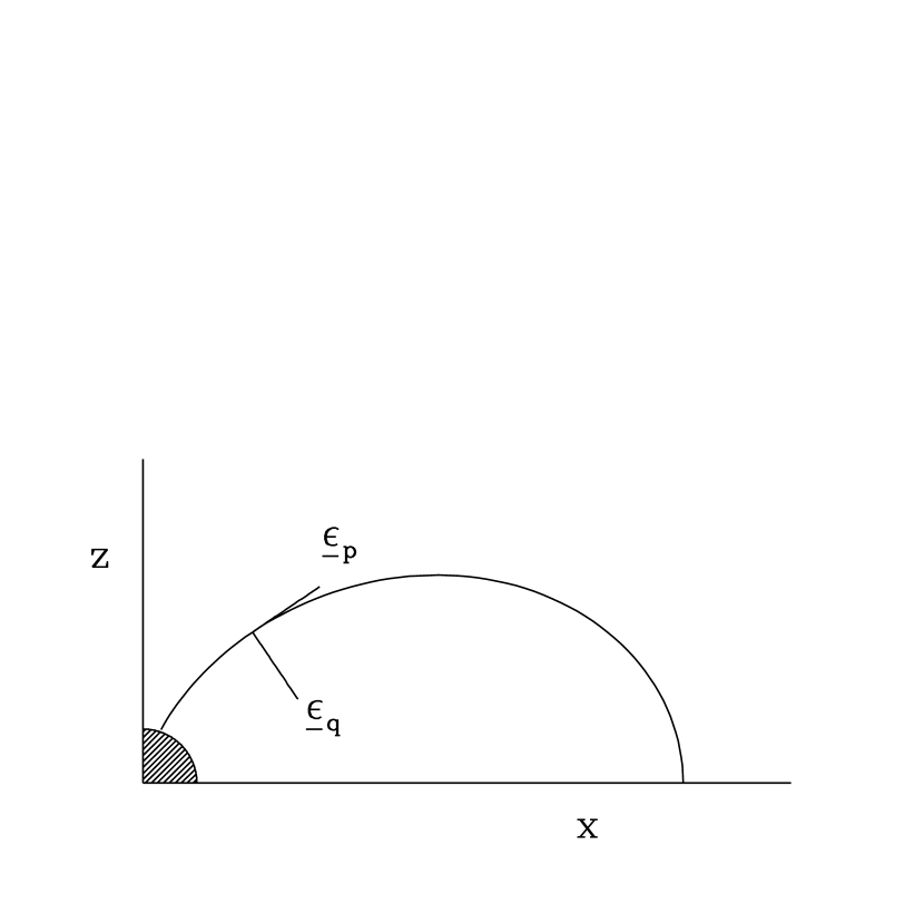
Figure 1: Schematic diagram showing the coordinates used here, for one quadrant of the poloidal plane. The star is shown in the lower left corner. The curve depicts one magnetic field line that connects the stellar surface to the inner edge of the disk. At each point along the field line, basis vectors describe the coordinate system. At one such point, the basis vectors are shown. The field lines correspond to lines of constant $q$, so the basis vector ${{\underline{\epsilon}}_{q}}$ = $\nabla q$ is perpendicular to the field line. The coordinate $p$ provides a measure of the distance along the field line, so that the basis vector ${{\underline{\epsilon}}_{p}}$ = $\nabla p$ points along the field line.

2 Construction of Coordinate Systems

In this treatment, we develop a series of coordinate systems that follow the magnetic field lines. We thus start with a given magnetic field configuration ${\bf B}(r,\theta)$, which we take to be axisymmetric (the magnetic field is poloidal, with no toroidal component, $B_{\phi}$ = 0). The origin is located at the center of the star. Since the star is expected to be rotating, the coordinate system co-rotates with the star, and is thus fixed. The effects of rotation are then incorporated by including (the usual) non-inertial terms in the equations of motion (see Section 3). By definition, coordinate systems are defined by scalar fields, which we denote here as $(p,q)$. If the magnetic field is curl-free (and hence current-free), then the field ${\bf B}$ can be written as the gradient of a scalar field. The coordinate $p$ specifies the distance along the field line and hence the gradient $\nabla p$ points in the direction of the field line. The coordinate $q$ is perpendicular so that $\nabla q\cdot\nabla p$ = 0. Notice that lines of constant $q$ correspond to the magnetic field lines; similarly, lines of constant $p$ correspond to equipotentials of the multipole field under consideration. The coordinates $(p,q)$ are thus orthogonal coordinates in the poloidal plane, and can be used instead of the more familiar spherical coordinates $(r,\theta)$. The azimuthal angle $\phi$ is the same for both cases and provides the third orthogonal coordinate. We could also use cartesian coordinates, where the pair $(x,z)$ define the poloidal plane.

As outlined above, this treatment neglects the azimuthal field component. In some systems, the presence of a twisted field component ($B_{\phi}\neq 0$) above the disk is necessary for maintaining balance in the angular momentum transport (Long et al. 2005). However, recent numerical simulations (e.g., Romanova et al. 2011, Long et al. 2011) indicate that the initial potential field structure is retained for regions within the disk truncation radius, so that our approximation ($B_{\phi}=0$) is viable. For completeness we note that, in general, the field will not strictly be a potential field when the azimuthal component is nonzero (although a potential field provides a good approximation); the azimuthal component also affects angular momentum transport.

Specification of a coordinate system requires not only the coordinates themselves, but also the basis vectors. For orthogonal coordinate systems, one can also use the scale factors. The set of covariant basis vectors ${{\underline{\epsilon}}_{j}}$ arises from the gradients of the scalar fields that define the coordinates (Weinreich 1998), in this case ${{\underline{\epsilon}}_{p}}\equiv\nabla p$ and ${{\underline{\epsilon}}_{q}}\equiv\nabla q$. Note that these quantities are basis vectors, rather than unit vectors, so that their length is not, in general, equal to unity. The corresponding scale factors $h_{j}$ are given by the relation

$$h_{j}=\left|{{\underline{\epsilon}}_{j}}\right|^{-1}\,.$$ (1)

The schematic diagram of Figure 1 depicts one magnetic field line and the basis vectors at one point along the field line. The coordinate $p$ measures the distance along the field line and the basis vector ${{\underline{\epsilon}}_{p}}=\nabla p$ points in the direction of the field line. The coordinate $q$ is constant along field lines, and thus labels both the field lines and the streamlines. The basis vector ${{\underline{\epsilon}}_{q}}=\nabla q$ is perpendicular to the field line.

In magnetically controlled accretion, one important geometrical effect is that the divergence operator takes a non-standard form. For orthogonal coordinate systems, the general form of the divergence operator is given by

$$\nabla\cdot{\bf V}={1\over h_{p}h_{q}h_{\phi}}\left[{\partial\over\partial p}\left(h_{q}h_{\phi}V_{p}\right)+{\partial\over\partial q}\left(h_{p}h_{\phi}V_{q}\right)\right]+{1\over\xi\sin\theta}{\partial V_{\phi}\over\partial\phi}\,.$$ (2)

The quantities $h_{p}$, $h_{q}$, and $h_{\phi}$ are the scale factors of the coordinate system, as defined by equation (1).

In this application, we consider the fields to be axisymmetric so that the $\phi$ derivatives vanish. Further, for flow along field lines, the vector fields (e.g., the velocity field) have only one component and depend on only one coordinate, so that the divergence operator collapses to the form

$$\nabla\cdot{\bf V}={1\over h_{p}h_{q}h_{\phi}}{\partial\over\partial p}\left(h_{q}h_{\phi}V_{p}\right)={1\over h_{p}}{\partial V_{p}\over\partial p}+{V_{p}\over h_{p}h_{q}h_{\phi}}{\partial\over\partial p}\left(h_{q}h_{\phi}\right)\,.$$ (3)

As shown in Appendix A, $h_{q}h_{\phi}$ = $h_{p}$ and $h_{p}\propto|{\bf B}|^{-1}$ (see Result 1 and the text below). For flow along the field lines, the divergence operator (3) thus has a form consistent with the well-known result that the effective area element of a moving fluid element varies inversely with the field strength (Parks 2004).

3 Fluid Equations for Magnetically Controlled Flow

In this treatment, we consider steady-state solutions and assume that the magnetic field structure is strong enough to dominate the flow. As a result, the magnetic field is held fixed and fluid elements must follow the field lines. The magnetic field is assumed to rotate with the star, so we work in a rotating reference frame with rotation rate ${{{\vec{\Omega}}}}=\Omega{{\hat{z}}}$. Under these approximations, the equations of continuity, force, and induction reduce to the forms

$$\nabla\cdot\left(\rho{{\bf u}}\right)=0\,,\qquad{{\bf u}}\cdot\nabla{{\bf u}}+\nabla\Psi+{{{\vec{\Omega}}}}\times({{{\vec{\Omega}}}}\times{\bf r})+{1\over\rho}\nabla P=0\,,\qquad{\rm and}\qquad{{\bf B}}={{\kappa}}\,\rho\,{{\bf u}}\,,$$ (4)

where the parameter ${{\kappa}}$ is constant along streamlines. Note that the magnetic field does not contribute a force along the field lines and that the Coriolis force also does not contribute. The correction to the effective gravity due to the rotating reference frame is included.

The velocity vector ${\bf u}$ follows the magnetic field lines. In the following sections, we construct coordinate systems such that one of the coordinates (denoted here as $p$) follows the field lines. As a result, the flow velocity has only one component, which points in the direction of the magnetic field ${{\hat{p}}}$ = $h_{p}\,{{\underline{\epsilon}}_{p}}$. We also assume that the thermodynamics of the flow can be modeled using a polytropic equation of state of the general form

$$P=K\rho^{1+1/n}\,,$$ (5)

where $n$ is the polytropic index. As shown below, however, the index $n$ must be relatively large in order for the flow to pass smoothly through the sonic transition. As a result, we consider the limiting case of an isothermal equation of state $n\to\infty$ for much of this paper.

3.1 Dimensionless Formulation

The problem can be re-formulated using dimensionless variables. Length scales can be measured in terms of the stellar radius $R_{\ast}$. We also define a reference scale $\rho_{1}$ for the density and use the corresponding sound speed $a_{1}$ as a reference velocity, given by $a_{1}^{2}=[\partial P/\partial\rho]_{1}$, or, equivalently,

$$a_{1}^{2}\equiv K\left(1+{1\over n}\right)\rho_{1}^{1/n}\,.$$ (6)

We can then define the following dimensionless quantities

$$\alpha\equiv{\rho\over\rho_{1}},\qquad u\equiv{|{\bf u}|\over a_{1}},\qquad\qquad\xi\equiv{r\over R_{\ast}},\qquad{\rm and}\qquad\psi\equiv{\Psi\over a_{1}^{2}}\,.$$ (7)

Note that $u$ is the (sonic) Mach number for isothermal flow. The stellar radius is typically $R_{\ast}\sim 10^{11}$ cm. The reference sound speed $a_{1}$ corresponds to that of the flow, which is launched from the inner edge of the disk; the appropriate temperature is that just above the disk surface, where the flow is exposed to UV heating, so that $T\sim{10^{4}}$ K and $a_{1}\sim 10$ km/s. The reference density scale $\rho_{1}$ depends on the mass accretion rate ${\dot{M}}$; for the standard value ${\dot{M}}\approx 10^{-8}M_{\odot}$ yr^-1, and for typical values for the other quantities (see Section 5.3), the reference density is given by $\rho_{1}/m_{p}=n_{1}\sim 3\times 10^{11}$ cm^-3.

Next we define a dimensionless parameter $b$ that measures the depth of the gravitational potential well,

$$b\equiv{GM_{\ast}\over R_{\ast}a_{1}^{2}}\approx 667\left({M_{\ast}\over 0.5M_{\odot}}\right)\left({R_{\ast}\over 10^{11}\,{\rm cm}}\right)^{-1}\left({a_{1}\over 10\,\,{\rm km}\,\,{\rm s}^{-1}}\right)^{-2}\,.$$ (8)

The depth of the potential well is thus expected to lie in the range $b\sim 500-1000$. Finally, we define a dimensionless parameter ${\omega}$ that measures the effects of rotation,

$${\omega}\equiv\left({\Omega R_{\ast}\over a_{1}}\right)^{2}=b\left({\Omega\over\,\,\Omega_{\ast}}\right)^{2}\,,$$ (9)

where $\Omega$ is the rotation rate of the star and $\Omega_{\ast}^{2}$ = $GM_{\ast}/R_{\ast}^{3}$ is the Keplerian rotation rate due to stellar gravity evaluated at the stellar surface. As a result, the rotation parameter can be written as ${\omega}=b\,(R_{\ast}/r_{\rm co})^{3}$, where $r_{\rm co}$ is the co-rotation radius. T Tauri stars exhibit a wide range of rotation periods $P=2\pi/\Omega\sim 2-12$ days (Herbst et al., 2007). For the median value $P\sim 6$ days, the co-rotation radius falls at $\sim 8R_{\ast}$, so we consider the range $r_{\rm co}\sim 6-10R_{\ast}$.

For simplicity we generally assume that the co-rotation radius $r_{\rm co}$ is coincident with the inner disk edge $r_{d}$ (so that ${\omega}=b/\xi_{d}^{3}$, where $\xi_{d}=r_{d}/R_{\ast}\sim 6-10$). In practice, accretion from the disk surface is launched from an annulus of finite extent $\Delta{r}$, although the width is generally narrow ($\Delta{r}<r$; see Section 5.3). If $\Delta{r}\ll{r}$, this finite width is not an issue. If the annulus extends beyond the co-rotation radius, the flow falls in the “propeller” regime where the star is spun down (Ustyugova et al. 2006). On the other hand, if the annulus extends inside the co-rotation radius, magnetic links to the regions of the disk spinning faster than the star, as well as accretion of disk material, act to spin-up the star, which will then increase its rotation rate and move the co-rotation radius further inward. However, induced changes in the location of the corotation radius, and/or the stellar spin, generally occur on long time scales.

In terms of the dimensionless fields defined above, the continuity equation takes the form

$$\alpha{\partial u\over\partial p}+u{\partial\alpha\over\partial p}=-{\alpha u\over h_{q}h_{\phi}}{\partial\over\partial p}\left(h_{q}h_{\phi}\right)\,,$$ (10)

and the force equation becomes

$$u{\partial u\over\partial p}+{\alpha^{1/n}\over\alpha}{\partial\alpha\over\partial p}-{\omega}\xi\sin\theta|\nabla p|^{-1}\left({{\hat{x}}}\cdot{{\hat{p}}}\right)=-{\partial\psi\over\partial p}=-{\partial\psi\over\partial\xi}{\partial\xi\over\partial p}=-{b\over\xi^{2}}{\partial\xi\over\partial p}\,.$$ (11)

These equations can be integrated immediately to obtain the solutions

$$\alpha uh_{q}h_{\phi}=\lambda\,,$$ (12)

and

$${1\over 2}u^{2}+n\alpha^{1/n}+\psi=\varepsilon+{\omega}\int\xi\sin\theta\left({{\hat{x}}}\cdot{{\hat{p}}}\right){dp\over|\nabla p|}\equiv\varepsilon+{\omega}I\,,$$ (13)

where the second equality defines the integral $I$ (this integral can be written in simple form; see Result 2 of Appendix A). The quantity $h_{q}h_{\phi}$ in equation (12) is proportional to the inverse of the magnetic field strength (consistent with the third part of equation [4]). The parameters $\lambda$ and $\varepsilon$ are constant along streamlines, but are not, in general, the same for all streamlines (they are functions of $q$).

3.2 Transitions through the Critical Points

Critical points in the flow arise when the fluid speed is equal to the transport speed. In general, magnetic media support three types of MHD waves and hence allow for three types of critical points. In the case where the flow is confined to follow magnetic field lines, the problem has only one possible critical point, which occurs where the flow speed equals the sound speed. In order for the flow to pass smoothly through this sonic point, only particular values of the constant $\lambda$ are allowed. The equations of motion (10) and (11) provide two equations for the two unknowns $\partial u/\partial p$ and $\partial\alpha/\partial p$; by solving for these quantities and requiring that the functions are continuous at the sonic point (e.g., Shu 1992), we find the required matching conditions

$$u^{2}=\alpha^{1/n}\qquad{\rm and}\qquad{\alpha^{1/n}\over h_{q}h_{\phi}}{\partial\over\partial p}\left(h_{q}h_{\phi}\right)+{\omega}\xi\sin\theta|\nabla p|^{-1}\left({{\hat{x}}}\cdot{{\hat{p}}}\right)\,={b\over\xi^{2}}{\partial\xi\over\partial p}\,.$$ (14)

Note that these expressions remain valid in the isothermal limit where $n\to\infty$ and hence $\alpha^{1/n}\to 1$. We must thus evaluate the geometrical factor $\cal G$ defined by

$${\cal G}\equiv{1\over h_{q}h_{\phi}}{\partial\over\partial p}\left(h_{q}h_{\phi}\right)={1\over h_{p}}{\partial h_{p}\over\partial p}\,,$$ (15)

where the second equality follows from Result 1 in Appendix A. Note that for radial flow in spherical coordinates, where $p$ = $\xi$, this factor would have the familiar form ${\cal G}=2/\xi$.

In general, the divergence operator, and the geometrical factor ${\cal G}$ have units of $p^{-1}$, but the coordinate $p$ is not necessarily a length scale. Nonetheless, we can define a dimensionless parameter ${\Upsilon}$ that measures the degree of divergence through the construction

$${\Upsilon}={\Upsilon}(\xi,\theta)=\xi H\,\left({\partial p\over\partial\xi}\right)^{-1}\,{\cal G}\,\quad\longrightarrow\quad{\Upsilon}(\xi)={\xi\over h_{p}}{\partial h_{p}\over\partial\xi}\,,$$ (16)

where the function $H$ is defined by equation (A16) in Appendix A. The intermediate expression is general, whereas the final equality applies to the specific case where the flow is confined to a field line so that the angle $\theta(\xi)$ is a known function of $\xi$. With the definition (16), the index ${\Upsilon}$ is of order unity and is a slowly varying function of the coordinates. Similarly, we define the function ${\Lambda}$ that specifies the rotational term in the force equation,

$${\Lambda}=\xi\sin\theta\,\left({\partial p\over\partial\xi}\right)^{-1}\left({{\hat{x}}}\cdot\nabla p\right)\,.$$ (17)

In terms of these functions, the matching condition at the sonic point takes the seemingly simple form

$$\alpha^{1/n}{{\Upsilon}\over\xi}+{\omega}{\Lambda}={b\over\xi^{2}}\,.$$ (18)

In general the quantities ${\Upsilon}$ and ${\Lambda}$ are functions of $(\xi,\theta)$. For flow along a magnetic field line, which are lines of constant $q$, the angle $\theta$ is a specified function of the radial coordinate, so that we obtain functions of a single variable ${\Upsilon}(\xi)$ and ${\Lambda}(\xi)$. In the isothermal limit $n\to\infty$, the density dependence drops out, so that all of the terms in equation (18) become known functions of the variable $\xi$. For a general polytropic index, the two equations of motion (evaluated at the sonic point), in conjunction with the two matching conditions, allow one to solve for the four unknowns $\xi_{s}$, $\alpha_{s}$, $u_{s}$, and $\lambda$. After eliminating the other three variables, the equation that specifies the sonic point has the form

$${\left(b-{\omega}{\Lambda}\xi^{2}\right)\over\xi{\Upsilon}}=\left\{2h_{p}^{-2}\left[\left(n+{1\over 2}\right){\left(b-{\omega}{\Lambda}\xi^{2}\right)\over\xi{\Upsilon}}-{\omega}I-{b\over\xi}+b-n\right]\right\}^{1/(2n+1)}\,.$$ (19)

This equation applies to steady polytropic flow that follows any magnetic field configuration, where the geometry is encapsulated in the index ${\Upsilon}(\xi)$ of the divergence operator, the scale factor $h_{p}$, the rotational term ${\Lambda}(\xi)$, and its integral $I$. The physical system is specified by the depth $b$ of the potential well, the rotational speed (through ${\omega}$), and the polytropic index $n$. Finally, the streamline of the flow is determined by the intersection point with the equatorial plane, where this point (often taken to be the inner disk edge $\xi_{d}$) specifies the value of the coordinate $q$. Equation (19) remains valid in the isothermal limit $n\to\infty$, where the right hand side of the equation becomes unity.

With the location of the sonic point $\xi_{s}$ specified by equation (19), the dimensionless mass accretion rate $\lambda$ for finite $n$ is given by

$$\lambda=h_{p}\left({b-{\omega}{\Lambda}\xi_{s}^{2}\over\xi_{s}{\Upsilon}}\right)^{n+1/2}\,,$$ (20)

where all of the quantities are evaluated at $\xi_{s}$. In the isothermal limit, accretion parameter $\lambda$ is specified implicitly through the transcendental equation

$$\ln\lambda-{1\over 2}\lambda^{2}=\ln h_{p}+{\omega}I+b\left({1\over\xi_{s}}-1\right)-{1\over 2}\,.$$ (21)

3.3 General Constraint on Steady Polytropic Flow

In this section, we derive a general constraint that must be met for steady transonic accretion to reach free-fall speeds in the inner limit. Here, the flow starts at the inner disk edge (at subsonic speed) and ends on the stellar surface (at supersonic speed). This result applies to polytropic flow that follows magnetic field lines. Let the integer $\ell$ denote the highest order multipole of the field near the stellar surface and let $n$ denote the polytropic index of the equation of state. We find that self-consistent transonic solutions must satisfy the requirement

$$n>\ell+{3\over 2}\,$$ (22)

in order to achieve (nearly) free-fall speeds in the inner limit. This constraint implies that, to leading order, the flow can be described using an isothermal equation of state.

The constraint of equation (22) can be derived as follows: In the limit $\xi\ll 1$, only the highest order multipole field contributes to the magnetic field. In this limit, the continuity equation reduces to the form

$$\alpha u=\lambda A\xi^{-(\ell+2)}\,,$$ (23)

where $A$ is a constant (for example, this constant has values $A$ = 2, $2{\Gamma}$, and 2 for the magnetic field configurations considered in Sections 4 and 5, and Appendix B, respectively). The force equation reduces to the form

$${1\over 2}u^{2}+n\alpha^{1/n}={b\over\xi}\,.$$ (24)

The combination of these two reduced equations of motion results in the expression

$${1\over 2}u^{2}+n\left(\lambda A\right)^{1/n}\xi^{-(\ell+2)/n}u^{-1/n}={b\over\xi}\,.$$ (25)

In order for the solutions to approach a free-fall form in the inner limit, the velocity field must approach the form $u^{2}\sim 2b/\xi$, which requires the first term to dominate the second in equation (25). Consistency thus requires

$$u^{2}\gg\alpha^{1/n}\qquad{\rm which}\,\,\,{\rm implies}\qquad{1\over\xi}\gg{1\over\xi^{(\ell+3/2)/n}}\,.$$ (26)

The requirement implies that $\ell+3/2<n$, as claimed in the constraint of equation (22).

We note that this argument applies for the limit where $\xi\to 0$. In practice, magnetically controlled accretion takes place over a limited range in radius, from the inner disk edge to the stellar surface, i.e., spanning only about a factor of 10 in radial scale. In order for the equation of state to be stiff enough to affect the accretion flow over this more limited range, the polytropic index $n$ must be larger than the value $\ell+3/2$, as given by equation (22).

In addition, for the case of dipole fields $\ell=1$, Koldoba et al. (2002) find that the behavior of accretions flows from disks onto magnetized stars has qualitatively different behavior when the polytropic index $n$ is smaller or larger than $n=5/2=\ell+3/2$ (the same threshold indicated by equation [22]). For $n>5/2$, the Mach number increases monotonically as the flow approaches the stellar surface (i.e., for decreasing radius); for $n<5/2$, the Mach number first increases and then decreases as the flow moves inward (see Koldoba et al. 2002 for further discussion).

The observational implications of this constraint are important: First we note that current observations indicate that transonic flow with free-fall speeds does take place. Further, observations of magnetic field signatures for T Tauri stars suggest that the octupole component provides the largest contribution near the stellar surface. As a result, we should take $\ell$ = 3, so that the constraint becomes $n>9/2$. From the inner disk edge to the stellar surface, the density can vary significantly, e.g., by a factor of $\sim 100$ for the models considered in this paper. Due to this constraint, however, the temperature (sound speed) could vary by at most a factor of $\sim 2.8$ (1.7). As a result, the flow is close to isothermal, and we consider the isothermal limit ($n\to\infty$) for most of this work. This approximation is consistent with previous modeling work (Hartmann et al., 1994), which finds that reasonable hydrogen line profiles can be obtained if the temperature profiles are roughly isothermal (except for an initial rise in temperature where the flow leaves the disk). On a related note, calculations of the thermal structure of accretion funnels (Martin 1996) indicate that the Ca II and Mg II ions have a strong cooling effect on the flow, i.e., they act as a thermostat and give rise to nearly isothermal conditions in the vicinity of the stellar surface.

3.4 Mass Accretion Rate

The discussion thus far has focused on one streamline at a time. This section shows how the streamlines add up to determine the mass accretion rate from the disk onto the star.

The total mass accretion rate ${\dot{M}}_{d}$ leaving the inner portion of the disk takes the form

$${\dot{M}}_{d}=2\int_{r_{d}}^{r_{2}}2\pi rdr\,\rho\,v\,=4\pi R_{\ast}^{2}\rho_{1}a_{1}\int_{\xi_{d}}^{\xi_{2}}\,\varpi d\varpi\,\alpha_{1}u_{1}=4\pi R_{\ast}^{2}\rho_{1}a_{1}\int_{\xi_{d}}^{\xi_{2}}\varpi d\varpi\lambda\,\left(h_{p}^{-1}\right)_{d}\,,$$ (27)

where $r_{d}$ is the inner disk edge, the accreting annulus extends from $r_{d}$ to $r_{2}$, and the variable $\varpi\equiv r/R_{\ast}$. The leading factor of 2 arises because material accretes from both the top and bottom surfaces of the disk. In the final equality we have used the boundary conditions that $\alpha$ = 1 and $u$ = $\lambda/h_{p}$ at the start of the trajectory, and the subscript indicates that the quantity is to be evaluated in the disk plane. The flow is assumed to leave the disk surface in the vertical (${{\hat{z}}}$) direction, consistent with the magnetic field line geometries of interest (primarily dipoles and octupoles). For the sake of completeness, however, we note that the flow is somewhat more complicated because the magnetic field threading the disk bends away from the vertical at the disk surface, and because the surface itself is not perfectly flat. As a result, material in the accretion flow must first climb over a potential maximum before leaving the disk and falling toward the star (Scharlemann 1978, Ghosh & Lamb 1979). In practice, of course, we see ample observational evidence for accretion columns and magnetically truncated disks (see Section 1 for references), so that material can readily leave the plane of the disk.

The streamlines, which follow the magnetic field lines, end on the stellar surface, where the mass accretion rate ${\dot{M}}_{\ast}$ onto the star is given by

$${\dot{M}}_{\ast}=2\int_{\mu_{1}}^{\mu_{2}}2\pi R_{\ast}^{2}\,d\mu\,\rho\,v\,\left({{\hat{r}}}\cdot{{\hat{p}}}\right)=4\pi R_{\ast}^{2}\,\rho_{1}a_{1}\,\int_{\mu_{1}}^{\mu_{2}}d\mu\,\left({{\hat{r}}}\cdot{{\hat{p}}}\right)_{\ast}\,\lambda\,\left(h_{p}^{-1}\right)_{\ast}\,,$$ (28)

where the subscripts denote that the quantities are to be evaluated at the stellar surface. The end points of integration $\mu_{1}$ and $\mu_{2}$ (where $\mu=\cos\theta$) are determined by the angles where the streamlines (field lines) starting at $\xi_{d}$ and $\xi_{2}$ intersect the stellar surface. The leading factor of 2 arises because accretion onto the star takes place into rings on both hemispheres. Notice that the dot product $({{\hat{r}}}\cdot{{\hat{p}}})$ must be included because, in general, the streamlines do not intersect the stellar surface in the radial direction.

In order for mass to be conserved, as required, the mass accretion flow leaving the disk surface, given by equation (27), must be the same as the mass accretion rate onto the stellar surface, given by equation (28). Comparison of the two expressions shows that they are equal if the integrals are equal. This equality holds and is shown in Appendix C (which thus provides a consistency check on this approach).

4 Magnetic Accretion with a Dipole Field

This section considers the field geometry to be that of a simple dipole. Although magnetic accretion with a dipole field has been addressed previously (e.g., Hartmann et al. 1994, Koldoba et al. 2002), we revisit the problem using our approach, which sets up the generalizations in the following section.

4.1 The Coordinate System

For the case of a pure dipole field, we use coordinates of the form

$$p=-\xi^{-2}\cos\theta\qquad{\rm and}\qquad q=\xi^{-1}\sin^{2}\theta\,,$$ (29)

where $\xi=r/R_{\ast}$ (see also Radoski 1967, Canalle et al. 2005, and Appendix A). The streamline (and hence magnetic field line) that intersects the disk at its inner edge is thus given by $q$ = $R_{\ast}/r_{d}$, so that this streamline corresponds to the trajectory $\xi R_{\ast}$ = $r_{d}\sin^{2}\theta$.

The covariant basis vectors ${{\underline{\epsilon}}_{j}}$ arise from the gradients of the scalar fields that define the coordinates. If we express these vectors in terms of the original spherical coordinates $(\xi,\theta,\phi)$, the basis takes the form

$${{\underline{\epsilon}}_{p}}=2\xi^{-3}\cos\theta\,{{\hat{r}}}+\xi^{-3}\sin\theta\,{{\hat{\theta}}}\,,$$ (30)

$${{\underline{\epsilon}}_{q}}=-\xi^{-2}\sin^{2}\theta\,{{\hat{r}}}+2\xi^{-2}\sin\theta\cos\theta\,{{\hat{\theta}}}\,,$$ (31)

and

$${{\underline{\epsilon}}_{\phi}}={1\over\xi\sin\theta}\,{{\hat{\phi}}}\,,$$ (32)

where the quantities $({{\hat{r}}},{{\hat{\theta}}},{{\hat{\phi}}})$ are the usual unit vectors for spherical coordinates. The scale factors thus become

$$h_{p}=\xi^{3}\left[4\cos^{2}\theta+\sin^{2}\theta\right]^{-1/2}\,,$$ (33)

$$h_{q}={\xi^{2}\over\sin\theta}\left[4\cos^{2}\theta+\sin^{2}\theta\right]^{-1/2}\,,$$ (34)

and

$$h_{\phi}=\xi\sin\theta\,.$$ (35)

The geometrical factor ${\cal G}$ in the divergence operator is thus

$${\cal G}=3\xi^{2}\cos\theta{8-5\sin^{2}\theta\over(4-3\sin^{2}\theta)^{2}}\,.$$ (36)

For flow along a field line (constant $q$), the effective index ${\Upsilon}$ of the divergence operator (see equation [16]) thus takes the form

$${\Upsilon}={\Upsilon}(\xi)={3\over 2}\,\left({8-5q\xi\over 4-3q\xi}\right)\,.$$ (37)

In the inner limit where $\xi\to 0$, the index ${\Upsilon}\to 3$, as expected for dipole geometry. For streamlines, and hence magnetic field lines, that connect the disk plane to the stellar surface, the product $q\xi\to 1$ where the streamlines intersect the disk. As a result, at the outer starting point of a streamline, the index approaches the not-so-obvious value ${\Upsilon}\to 9/2$. Finally, for dipole field configurations, the rotational term ${\Lambda}$ (see equation [17]) takes the simple form

$${\Lambda}={\Lambda}(\xi)={3\over 2}q\xi^{2}\,.$$ (38)

4.2 Isothermal Accretion Flow

We now consider isothermal accretion flow. For a given streamline labeled by the coordinate $q$, we can eliminate the angular dependence from the equation of motion. Even though the fluid fields are functions of the coordinate $p$ only, the resulting expressions are simpler in terms of the radial variable $\xi(p)$. This change of variables is transparent as long as $\xi$ is monotonic as a function of $p$. The equations of motion thus take the form

$$\alpha{\partial u\over\partial\xi}+u{\partial\alpha\over\partial\xi}=-\alpha\,u\,{{\Upsilon}\over\xi}=-\alpha\,u\,{3\over 2\xi}\,{8-5q\xi\over 4-3q\xi}\,,$$ (39)

and

$$u{\partial u\over\partial\xi}+{1\over\alpha}{\partial\alpha\over\partial\xi}=-{b\over\xi^{2}}+{\omega}\,{\Lambda}\,=-{b\over\xi^{2}}+{3\over 2}\,{\omega}\,q\,\xi^{2}\,.$$ (40)

The matching condition for the sonic point takes the form

$$3\xi\,{8-5q\xi\over 4-3q\xi}=2b-3\,{\omega}\,q\,\xi^{4}\,.$$ (41)

For the case where the inner disk edge corresponds to the co-rotation point, the solution to equation (41) lies just inside the point $\xi_{0}=(2/3)^{1/4}$ $r_{d}/R_{\ast}$. We denote the sonic point as $\xi_{s}$.

The equations of motion can be integrated to take the forms

$$\alpha u=\lambda(q\xi)^{-3}\left(4-3q\xi\right)^{1/2}\,,$$ (42)

and

$${1\over 2}u^{2}+\ln\alpha=\varepsilon+{b\over\xi}+{1\over 2}{\omega}q\xi^{3}\,.$$ (43)

At the inner disk edge, $\xi=1/q$ and $\alpha=1$; the integration constant $\lambda$ in equation (42) is defined so that $u=\lambda$ at this boundary. The second constant $\varepsilon$ from equation (43) is then given by

$$\varepsilon={1\over 2}\lambda^{2}-{3\over 2}bq\,,$$ (44)

where we have assumed that the inner disk edge, the launching point of the flow, and the co-rotation radius coincide (so that ${\omega}=bq^{3}$). Using this result to specify $\varepsilon$ and taking the logarithm of the continuity equation (42), we find the following implicit specification of the remaining constant $\lambda$:

$$\ln\lambda-{1\over 2}\lambda^{2}=3\ln\xi_{s}-{1\over 2}\ln(4-3\xi_{s})-{1\over 2}+b\left({1\over\xi_{s}}+{1\over 2}\xi_{s}^{3}-{3\over 2}\right)\,.$$ (45)

This equation has two roots for $\lambda$, one with $\lambda<1$ and another with $\lambda>1$. The accretion solutions of interest here start with subsonic speeds at $\xi=\xi_{d}=1/q$, where $u=\lambda$, so we must take the smaller root ($\lambda<1$).

Figure 2: Dimensionless fluid fields for accretion solution using a pure dipole geometry and an isothermal equation of state. The inner disk edge lies at $\xi=\xi_{d}$ = 10 and the stellar surface corresponds to $\xi=\xi_{\ast}$ = 1.0. For dimensionless depth of the gravitational potential well $b$ = 500, the velocity field $u$ is shown by the solid curve and the density $\alpha$ is shown by the dashed curve. The corresponding solutions for $b$ = 1000 are shown by the dotted curves. For the reference values $n_{1}$ = $3\times 10^{11}$ g cm^-3 and $a_{1}$ = 10 km s^-1, these solutions have physical speeds $u_{\ast}\approx$ 290 km s^-1 (410 km s^-1) and number densities $n_{\ast}\approx 2\times 10^{12}$ g cm^-3 ($5\times 10^{11}$ g cm^-3) at the stellar surface for $b$ = 500 (1000).

For flow that passes smoothly through the sonic point, we can find the dimensionless fluid fields $\alpha$ and $u$. These profiles are plotted in Figure 2 for two choices of the dimensionless depth $b$ of the gravitational potential well of the star. Notice that the density field initially decreases inward from the starting point (at the disk edge), but eventually increases. This behavior can be understood by finding the limiting form of the solutions for the regimes $|1-\xi|\ll 1$ and $\xi\ll 1$, as shown in the following subsection.

4.3 Limiting Forms for the Flow Solutions

In the regime $|1-q\xi|\ll 1$, we define $\eta$ such that $q\xi=1-\eta$, where $\eta\ll 1$ (and $q=1/\xi_{d}$). The equations of motion take the form

$$\alpha u=\lambda\left(1+{9\over 2}\eta\right)\,,$$ (46)

and

$${1\over 2}u^{2}+\ln\alpha={1\over 2}\left(\lambda^{2}-bq\eta\right)\,,$$ (47)

where we have kept only the leading order terms (in $\eta$). Working to leading order (in $\eta$), we find

$$u\approx\lambda\exp\left[{1\over 2}\eta(bq+9)\right]\qquad{\rm and}\qquad\alpha=\left(1+{9\over 2}\eta\right)\exp\left[-{1\over 2}\eta(bq+9)\right]\,.$$ (48)

These expressions can be expanded further, keeping only the leading order terms in $\eta$, to obtain the forms

$$u\approx\lambda\left[1+{1\over 2}\eta(bq+9)\right]\qquad{\rm and}\qquad\alpha\approx 1-{1\over 2}bq\eta\,.$$ (49)

The initial decrease in the density field is thus clear (see Figure 2).

In the opposite limit where $\xi\ll 1$, the equation of motion reduce to the forms

$$\alpha u=2\lambda q^{-3}\xi^{-3}\,,$$ (50)

and

$${1\over 2}u^{2}+\ln\alpha={b\over\xi}\,.$$ (51)

To leading order, the dimensionless fluid fields become

$$u\approx\left({2b\over\xi}\right)^{1/2}\qquad{\rm and}\qquad\alpha\approx\left({2\over b}\right)^{1/2}{\lambda q^{-3}\over\xi^{5/2}}\,.$$ (52)

The fluid fields thus increase as $\xi\to 0$.

One can also show that the velocity field $u(\xi)$ is monotonic for this problem. If we use the equations of motion to eliminate the density $\alpha$ in favor of the velocity $u$, we obtain

$${1\over 2}u^{2}-\ln u=\varepsilon+{b\over\xi}+{1\over 2}\,b\,q^{4}\,\xi^{3}-\ln\lambda+3\ln(q\xi)-{1\over 2}\ln\left[4-3q\xi\right]\,.$$ (53)

Taking the derivative of both sides we find

$$\left(u-{1\over u}\right){du\over d\xi}=-{b\over\xi^{2}}+{3\over 2}\,b\,q^{4}\,\xi^{2}+{3\over\xi}+{3q\over 2(4-3q\xi)}\equiv F(\xi)\,.$$ (54)

One can show that the function $F(\xi)$, the right hand side of the above expression, is monotonically increasing on the interval $0\leq\xi\leq 1$, has a zero at the sonic point, is positive for $\xi=1$ and is negative in the limit $\xi\to 0$. These properties, in conjunction with equation (54) imply that $u$ is monotonic and decreasing. Note that the statement that $u$ is decreasing means that the velocity increases as fluid elements approach the star.

5 Magnetic Accretion with Dipole plus Octupole Field

In this section we consider the stellar magnetic field to have both dipole and octupole components. The magnetic field thus takes the form

$${\bf B}={B_{\rm oct}\over 2}\xi^{-5}\left[\left(5\cos^{2}\theta-3\right)\cos\theta\,{{\hat{r}}}+{3\over 4}\left(5\cos^{2}\theta-1\right)\sin\theta\,{{\hat{\theta}}}\right]+{B_{\rm dip}\over 2}\xi^{-3}\left(2\cos\theta\,{{\hat{r}}}+\sin\theta\,{{\hat{\theta}}}\right)\,,$$ (55)

where $\xi=r/R_{\ast}$ is the dimensionless radius. The leading factors of 1/2 (for both the dipole and octupole terms) are included to be consistent with the convention of Gregory et al. (2010). If we scale out the dipole field strength, the relative size of the octupole contribution is given by the dimensionless parameter

$${\Gamma}\equiv{B_{\rm oct}\over B_{\rm dip}}\,.$$ (56)

Observations of the signatures of magnetic accretion onto T Tauri stars indicate that the parameter ${\Gamma}$ lies in the range $0\leq{\Gamma}\leq 10$. For example, the young stars V2129 Oph (Donati et al. 2007) and BP Tau (Donati et al. 2008) are observed to have field parameter ${\Gamma}=1-4$. The star AA Tau (Donati et al. 2010b) has a nearly dipole field with ${\Gamma}\approx 0.25$, whereas TW Hya has a much larger octupole component with ${\Gamma}\approx 4$ observed at one epoch and ${\Gamma}\approx 6$ found at another (Donati et al. 2011b).

5.1 The Coordinate System

With the configuration of equation (55), the magnetic field is current-free and curl-free, and can be written as the gradient of a scalar field (see Appendix A). The first scalar field $p$ of the coordinate system takes the form

$$p=-{1\over 4}\xi^{-4}{\Gamma}\left(5\cos^{2}\theta-3\right)\cos\theta-\xi^{-2}\cos\theta\,.$$ (57)

The gradient $\nabla p$ points in the direction of the magnetic field. Next we construct the perpendicular vector field $\nabla q$, where the scalar field $q$ provides the second coordinate and is given by

$$q={1\over 4}\xi^{-3}{\Gamma}\left(5\cos^{2}\theta-1\right)\sin^{2}\theta+\xi^{-1}\sin^{2}\theta\,.$$ (58)

The scalar fields $(p,q)$ represent orthogonal coordinates in the poloidal plane and are used instead of the spherical coordinates $(\xi,\theta)$. In this version of the problem, the magnetic field is axisymmetric about the ${{\hat{z}}}$ axis, so that the usual azimuthal coordinate $\phi$ is the third scalar field. Note that both $p$ and $q$ are dimensionless.

Next we find the covariant basis vectors ${{\underline{\epsilon}}_{j}}$, which can be written in terms of the original coordinates $(\xi,\theta)$, so that the basis takes the form

$${{\underline{\epsilon}}_{p}}=\left[\xi^{-5}{\Gamma}\left(5\cos^{2}\theta-3\right)+2\xi^{-3}\right]\cos\theta\,{{\hat{r}}}+\left[{3\over 4}\xi^{-5}{\Gamma}\left(5\cos^{2}\theta-1\right)+\xi^{-3}\right]\sin\theta\,{{\hat{\theta}}}\,,$$ (59)

and

$${{\underline{\epsilon}}_{q}}=-\left[{3\over 4}\xi^{-4}{\Gamma}\left(5\cos^{2}\theta-1\right)+\xi^{-2}\right]\sin^{2}\theta\,{{\hat{r}}}+\left[\xi^{-4}{\Gamma}\left(5\cos^{2}\theta-3\right)+2\xi^{-2}\right]\sin\theta\cos\theta\,{{\hat{\theta}}}\,,$$ (60)

where the third basis vector ${{\underline{\epsilon}}_{\phi}}$ is given by equation (32).

It is useful to define ancillary functions

$$f={\Gamma}\left(5\cos^{2}\theta-3\right)+2\xi^{2}\qquad{\rm and}\qquad g={3\over 4}{\Gamma}\left(5\cos^{2}\theta-1\right)+\xi^{2}\,.$$ (61)

With these definitions, we can write the magnitudes of the basis vectors in the forms

$$|{{\underline{\epsilon}}_{p}}|^{2}=\xi^{-10}\left[f^{2}\cos^{2}\theta+g^{2}\sin^{2}\theta\right]\,,$$ (62)

and

$$|{{\underline{\epsilon}}_{q}}|^{2}=\xi^{-8}\sin^{2}\theta\left[g^{2}\sin^{2}\theta+f^{2}\cos^{2}\theta\right]\,.$$ (63)

The corresponding scale factors thus become

$$h_{p}=\xi^{5}\left[f^{2}\cos^{2}\theta+g^{2}\sin^{2}\theta\right]^{-1/2}\,,$$ (64)

and

$$h_{q}={\xi^{4}\over\sin\theta}\left[g^{2}\sin^{2}\theta+f^{2}\cos^{2}\theta\right]^{-1/2}\,,$$ (65)

where the third scale factor $h_{\phi}$ is given by equation (35).

This specification of the divergence operator is implicit. One could invert equations (57) and (58), and then write the spherical coordinates $(\xi,\theta)$, the scale factors $(h_{p},h_{q},h_{\phi})$, and the ancillary functions $(f,g)$ as functions of the new coordinates $(p,q)$. However, the definitions of $(p,q)$ are nontrivial functions of $(\xi,\theta)$, so that inversion is complicated and unwieldy. For clarity, we leave this construction in implicit form.

Figure 3: Magnetic field lines centered on the star for configurations with both a dipole and an octupole contribution. For this case, the dimensionless parameter ${\Gamma}$ = 10. The star is shown in the lower left of the figure, the disk is shown as a wedge just above the $x$-axis. A collection of lines of constant $p$, the surface orthogonal to the field lines, is also shown.

5.2 Results for Flow Along a Field Line

The lines of constant $q$ define the trajectories of fluid elements following along magnetic field lines. Here we are interested in the subset of field lines that intersect the equatorial plane and hence intersect the disk. Note that in a fixed poloidal plane, and close to the stellar surface, the axisymmetric dipole plus octupole fields have three regions of closed field line loops between the north and south pole of the star; the higher latitude regions that do not intersect the disk are not considered here. By inverting equation (58), we can find the angle $\theta$ as a function of radius $\xi$ along a field line:

$$\sin^{2}\theta={2\over 5{\Gamma}}\left\{(\xi^{2}+{\Gamma})-\left[(\xi^{2}+{\Gamma})^{2}-5{\Gamma}q\xi^{3}\right]^{1/2}\right\}\,.$$ (66)

For the streamlines of interest, we must choose the negative sign for the discriminant (as shown below in equation [71], for sufficiently large values of ${\Gamma}$, streamlines that intersect the disk have $q<0$, and we must use the opposite sign). The ancillary functions can then be written as a function of the radial coordinate only:

$$f(\xi)=2\left[(\xi^{2}+{\Gamma})^{2}-5{\Gamma}q\xi^{3}\right]^{1/2}$$ (67)

and

$$g(\xi)={3\over 2}\left\{{\Gamma}+\left[(\xi^{2}+{\Gamma})^{2}-5{\Gamma}q\xi^{3}\right]^{1/2}\right\}-{1\over 2}\xi^{2}\,.$$ (68)

With these definitions, we can find the rotational function ${\Lambda}$ (see equation [17]) for flow along a field line,

$${\Lambda}(\xi)={2\xi\over 5{\Gamma}}\left\{(\xi^{2}+{\Gamma})-\left[(\xi^{2}+{\Gamma})^{2}-5{\Gamma}q\xi^{3}\right]^{1/2}\right\}\left\{1+{g(\xi)\over f(\xi)}\right\}\,.$$ (69)

The index ${\Upsilon}$ (from equation [16]) takes the form

$${\Upsilon}(\xi)=5-\left[f^{2}+(g^{2}-f^{2}){1\over 5{\Gamma}}\left(2\xi^{2}+2{\Gamma}-f\right)\right]^{-1}\times\qquad\qquad\qquad\qquad\qquad\qquad$$ (70)

$$\,\qquad{\xi\over 5{\Gamma}}\left\{5{\Gamma}ff_{\xi}+\left[g\left({3\over 4}f_{\xi}-\xi\right)-ff_{\xi}\right]\left(2\xi^{2}+2{\Gamma}-f\right)+(g^{2}-f^{2})\left(2\xi-{1\over 2}f_{\xi}\right)\right\}\,,$$

where $f(\xi)$ and $g(\xi)$ are given by equations (67, 68), and where $f_{\xi}=df/d\xi$.

The index ${\Upsilon}$ is a slowly varying function of the radius $\xi$, or, equivalently, the position $p(\xi)$ along the field line. The index function ${\Upsilon}$ is plotted in Figure 4 for varying values of the parameter ${\Gamma}$ that sets the relative strength of the octupole component. The solid curves show the index ${\Upsilon}(\xi)$ for parameter values ${\Gamma}$ from $10^{-2}$ (bottom) to $10^{3/2}$ (top). The dashed curve shows the limiting case of a pure dipole field. In the limit $\xi\to 0$, the index ${\Upsilon}\to 5$, as expected for an octupole field. For a pure dipole field (dashed curve), the limiting value ${\Upsilon}\to 3$. Near the inner disk edge, the index is somewhat larger than the value ${\Upsilon}$ = 9/2 expected for a dipole. For the intermediate regime in $\xi$, the index first decreases as $\xi$ decreases (toward the dipole value of 3), but the index increases closer to the star as the octupole contribution dominates. For sufficiently large values of ${\Gamma}\gg 1$, the octupole component dominates the field even near the inner disk edge; for this regime, the value of the index approaches ${\Upsilon}$ = 15/2 (from equation [70] in the limit ${\Gamma}\to\infty$). Notice also that for the value ${\Gamma}\sim 30$ (e.g., the top curve in Figure 4), the compromise between the dipole and octupole terms leads to the index being nearly constant with value ${\Upsilon}\approx 5$.

Figure 4: Index ${\Upsilon}$ of the divergence operator (see equations [16] and [70]) for magnetic field configurations with both dipole and octupole components. The relative strength of the octupole component ${\Gamma}$ has values given by $\log_{10}{\Gamma}$ = 3/2, 1, 1/2, 0, –1/2, and –1 (from top to bottom). The dashed curve shows the limiting case of a pure dipole field where ${\Gamma}\to 0$. The heavy solid line at $\xi$ = 1 marks the surface of the star, where accretion flow stops; the curves continue inward to smaller values of $\xi$ to illustrate the asymptotic behavior of ${\Upsilon}(\xi)$.

The field lines cross the equatorial plane where $\sin\theta=1$ and $\cos\theta=0$ (where the fluid trajectories start). The value of $q$ that leads to plane-crossing at radius $\xi_{d}$ is thus given by

$$q={1\over\xi_{d}}\left(1-{{\Gamma}\over 4\xi_{d}^{2}}\right)\,.$$ (71)

The dimensionless truncation radius $\xi_{d}\sim 10$, so we expect $q\sim 1/10$ for field lines that thread the disk. If the octupole contribution is too large, ${\Gamma}>4\xi_{d}^{2}\sim 100$, the field lines that intersect the disk would have $q<0$ and the sign of the discriminant in equation (66) must change. T Tauri systems are expected to have ${\Gamma}\,\raise 1.29167pt\hbox{$<$}\kern-7.5pt\lower 3.01385pt\hbox{$\sim$}\,10$, so this complication should not arise.

Using the result $q\ll 1$, we can find an approximate expression for the co-latitude on the star where fields lines starting at the disk truncation point reach the stellar surface, i.e.,

$$\sin^{2}\theta_{\ast}={q\over 1+{\Gamma}}+{\cal O}(q^{2})={1\over\xi_{d}(1+{\Gamma})}+{\cal O}\left(\xi_{d}^{-2}\right)\,.$$ (72)

The second equality uses equation (71) to write $q$ in terms of the disk truncation radius $\xi_{d}$. This result shows that the field lines that connect the disk truncation to the star must meet the stellar surface near the pole $(\theta_{\ast}\ll{1})$. Increasing the octupole contribution (via increasing ${\Gamma}$) decreases the angle $\theta_{\ast}$ even further.

We can also find the ratio of areas. Let ${\cal A}_{d}$ be the area of an annulus on the disk. In the limit of a thin annulus with width $\Delta\xi$, the area ${\cal A}_{d}$ = $2\pi\xi(\Delta\xi)$. This area gets funneled onto the stellar surface over a much smaller area ${\cal A}_{\ast}$ given by

$${\cal A}_{\ast}=2\pi\left[\cos\theta_{\ast 2}-\cos\theta_{\ast 1}\right]\,.$$ (73)

This expression does not include the dot product ${{\hat{r}}}\cdot{{\hat{p}}}$, which takes into account the non-radial direction of the incoming material (equation [28] and Appendix C). Since the angle $\theta_{\ast}\ll{1}$, the dot product is close to unity, ${{\hat{r}}}\cdot{{\hat{p}}}\approx 1-(3{\Gamma}+1)^{2}/(8\xi_{d}[{\Gamma}+1]^{3})+\dots$, and can be neglected to leading order. Using the above results, we can evaluate the ratio of areas to find

$${{\cal A}_{\ast}\over{\cal A}_{d}}={1\over 2\,(1+{\Gamma})\,\xi_{d}^{3}}\left\{1+{\cal O}\left(\xi_{d}^{-2}\right)+{\cal O}\left([\Delta\xi]^{2}\right)\right\}\,\,.$$ (74)

This leading order expression shows that the ratio of areas decreases inversely with the increase in field strength, which increases as $\xi^{-3}$ from the dipole contribution and includes an extra factor of $(1+{\Gamma})$ at the stellar surface due to the octupole component.

In the limit of small $\xi$, we can find asymptotic forms for the velocity and density fields. As long as the equation of state is not too stiff, the dimensionless fluid fields approach the form

$$u\sim\left({2b\over\xi}\right)^{1/2}\qquad{\rm and}\qquad\alpha\sim\left({2\over b}\right)^{1/2}\lambda\,({\Gamma}+1)\,\xi^{-9/2}\,.$$ (75)

These forms are valid when the polytropic index $n>9/2$ (see Section 3.3). For flow with $n<9/2$, free-fall velocities are not realized.

Figure 5: Dimensionless fluid fields for the velocity $u$ (solid curve) and density $\alpha$ (dashed curve) for accretion solution with both dipole and octupole components. In these units, the inner disk edge corresponds to $\xi$ = $\xi_{d}$ = 10 and the stellar surface lies at $\xi=\xi_{\ast}$ = 1. The relative strength of the octupole component is set by the parameter ${\Gamma}$ = 10, and the dimensionless depth of the gravitational potential well $b$ = 500. The dotted curves show the corresponding solution for a dipole field (in the limit ${\Gamma}\to 0$). For the reference values $n_{1}$ = $3\times 10^{11}$ g cm^-3 and $a_{1}$ = 10 km s^-1, these solutions have speeds $u_{\ast}\approx$ 290 km s^-1 at the stellar surface; the corresponding number densities are $n_{\ast}\approx 2\times 10^{12}$ g cm^-3 for the pure dipole and $n_{\ast}\approx 2\times 10^{13}$ g cm^-3 for the dipole/octupole configuration.

5.3 Accretion Solutions

Figure 5 shows the density and velocity fields for a typical system with magnetic octupole parameter ${\Gamma}$ = 10 and dimensionless depth of the gravitational potential $b$ = 500. The solid curve shows the dimensionless velocity field $u(\xi)$ and the dashed curve shows the corresponding density profile $\alpha(\xi)$. For comparison, the dotted curves show the profiles for the same system with a pure dipole field. Since the dipole contribution dominates the magnetic field at the inner disk edge, and since the sonic point falls relatively near the edge, the location of the sonic point $\xi_{s}$ and the mass accretion constant $\lambda$ are only weakly dependent on the parameter ${\Gamma}$. Specifically, the sonic point $\xi_{s}\approx$ 8.80 for ${\Gamma}$ = 10, compared with $\xi_{s}\approx$ 8.87 for ${\Gamma}\to 0$; similarly, the parameter $\lambda\approx$ 0.0877 for ${\Gamma}$ = 10, compared with $\lambda\approx$ 0.113 for the limit ${\Gamma}\to 0$. Notice, however, this statement no longer holds if the octupole component dominates the magnetic field at the inner disk edge.

The most important difference between the two field configurations (with solutions shown in Figure 5) is that the density increases near the stellar surface more rapidly in the presence of an octupole component; here the density is larger than that of the dipole limit by a factor of $\sim 9.5$. Equation (75) suggests that the density should be larger than that of the dipole case by a factor of $(1+{\Gamma})=11$; this factor is somewhat larger than the value (9.5) depicted in Figure 5 because the solutions are not fully in the $\xi\to 0$ limit. Nonetheless, the inclusion of octupole field components allows the flow densities at the stellar surface to be greater by an order of magnitude compared to those from the dipole limit.

The physical value of the flow density at the stellar surface, before the accretion shock, can be estimated as follows. The mass accretion rate can be written in the approximate form

$${\dot{M}}=2\pi\rho_{1}a_{1}(r_{2}+r_{d})(r_{2}-r_{d}){\langle\lambda\rangle}\,,$$ (76)

where ${\langle\lambda\rangle}$ is normalized so that $u=\lambda$ at the inner disk edge and the mean value is taken to account for possible variations over the range of launching radii on the disk surface. It is useful to define a dimensionless width of the annulus where the flow originates, i.e., $w\equiv(r_{2}-r_{d})/r_{d}$. The number density $n_{1}$ at the start of the flow can then be written in the form

$$n_{1}={3\times 10^{11}\,{\rm g}\,{\rm cm}^{-3}\over(1+w/2)w}\left({{\dot{M}}\over 10^{-8}\,M_{\odot}\,{\rm yr}^{-1}}\right)\left({a_{1}\over 10\,{\rm km}\,{\rm s}^{-1}}\right)^{-1}\left({{\langle\lambda\rangle}\over 0.1}\right)^{-1}\left({r_{d}\over 10^{12}\,{\rm cm}}\right)^{-2}\,.$$ (77)

For dipole field configurations (see Figure 2), the number density $n_{\ast}$ at the stellar surface is larger than the initial density $n_{1}$ by a factor of $1-10$, so that $n_{\ast}\approx 10^{12}$ g cm^-3 (where we have taken $(1+w/2)w\sim 1$). For field configurations with octupole contributions, the number density is larger by another factor of $\sim(1+{\Gamma})$ (see Figure 5), so we expect $n_{\ast}\approx 10^{13}$ g cm^-3 for systems with substantial octupole components. The densities could be even larger if the initial annulus on the disk is narrow ($w\ll 1$).

For comparison, coronal densities for T Tauri stars are estimated to be of order $n_{cor}\sim 10^{9}-10^{11}$ g cm^-3 (Ness et al., 2004; Kastner et al., 2004), and these values are considered too low to produce the observed soft X-ray exess emission from these sources (Brickhouse et al., 2010). The X-ray emission can arise from shock heated plasma with temperatures $T\sim{3}\times 10^{6}$ K and densities $n\sim 10^{11}-10^{13}$ g cm^-3 (Argiroffi et al., 2011). These required densities are thus comparable to those expected from accretion flow (see above); more significantly, octupole contributions ${\Gamma}\neq 0$ may be necessary to explain the upper end of this range.

The expected accretion hot spot temperature $T_{S}$ can be written in terms of the other system parameters such that

$$T_{S}^{4}={GM_{\ast}{\dot{M}}\over R_{\ast}\sigma_{B}{\cal A}_{\ast}}\left(1-{R_{\ast}\over r_{d}}\right)={2\over\pi}\,\,{\xi_{d}^{3}(1+{\Gamma})\over{w(2+w)}}\,\,{GM_{\ast}{\dot{M}}\over\sigma_{B}R_{\ast}r_{d}^{2}}\left(1-{1\over\xi_{d}}\right)\,,$$ (78)

where $\sigma_{B}$ is the Stefan-Boltzmann constant, and the other quantities have been defined previously. Note that $T_{S}$ is the hot spot temperature at the end of the accretion flow where material arrives at the star and generates an optically thick shock. For the same physical values used to evaluate equation (77), we obtain $T_{S}\approx 7000$ K $(1+{\Gamma})^{1/4}$. Even for a strong octupole component, ${\Gamma}\sim 10$, the hot spot temperature is only $T_{S}\sim 12,700$ K. As a result, the hot spot temperatures for accretion flow along non-dipolar magnetic field lines remain consistent with the constraints established by Muzerolle et al. (2001) from line profile modeling, line ratios, and continuum emission constraints (see their Figure 16 and associated discussion). We note that the higher temperatures derived form X-ray observations of He-like line triplets (e.g., Argiroffi et al. 2011), and discussed in the previous paragraph, refer to the hotter post-shock regions. Although a full treatment of X-ray signatures is beyond the scope of this present work, other studies have suggested that emitted X-rays from the accretion shock could be absorbed within the accretion funnel (Sacco et al. 2010).

Figure 6: Dimensionless mass accretion parameter $\lambda$ as a function of the dimensionless depth $b$ of the gravitational potential well of the star. The magnetic field has both dipole and octupole contributions, where the parameter ${\Gamma}$ specifies the relative strength of the octupole component. The curves show $\lambda(b)$ for varying values ${\Gamma}$ = 30 (dot-dashed), 10 (solid), 3 (dotted), and in the pure dipole limit ${\Gamma}\to 0$ (dashed).

Figure 6 shows the mass accretion parameter $\lambda$ as a function of the depth $b$ of the stellar gravitational potential well. Curves are shown for a range of values for the parameter ${\Gamma}$ that sets the relative strength of the octupole component of the magnetic field. As shown in the figure, increasing the strength of the octupole contribution results in a decrease in the mass accretion $\lambda$. For all values of ${\Gamma}$, the parameter $\lambda$ decreases in both the limit of large $b$ and the limit of small $b$. For sufficiently large $b$, Figure 6 shows that the accretion parameter $\lambda$ is an exponentially decreasing function of the gravitational potential $b$. This behavior can be understood as follows: In this regime, the matching condition for the sonic point from equation (19) reduces to the form ${\omega}{\Lambda}\xi^{2}=b$; since ${\omega}\propto{b}$, the location of the sonic point $\xi_{s}$ becomes independent of the potential $b$. The mass accretion parameter is specified through equation (21), which takes the form $\ln\lambda=A-Cb$, where $A$ and $C$ are constant and $C=1-1/\xi_{s}>0$. The mass accretion parameter is then given by $\lambda\sim\exp[-Cb]$, as depicted in Figure 6.

6 Magnetic Truncation Radius

In these accreting systems, the circumstellar disk is (indirectly) observed to have an inner boundary at radius $r_{d}>R_{\ast}$. Further, the inner disk can be truncated at radius $r_{T}$ where the stress due to the stellar magnetic field is large enough to remove angular momentum from the Keplerian flow (for further discussion, see Ghosh & Lamb 1979, Königl 1991, Shu et al. 1994). Here we assume that $r_{d}=r_{T}$, but more complicated possibilities remain. The requirement of disk truncation implies a constraint on the magnetic field of the form

$$B^{2}\left(r,\theta={\pi\over 2}\right)\approx 4\pi\rho v^{2}\equiv\alpha{{\dot{M}}\over r^{2}}\left({GM_{\ast}\over r}\right)^{1/2}\,,$$ (79)

where $\alpha$ is a dimensionless parameter of order unity; for example, recent numerical simulations (Long et al. 2005) suggest that $\alpha$ = 1/2 (see also the review of Bouvier et al. 2007, and references therein). This parameter incorporates the difference between exact equality in the two sides, the difference between the flow speed and the free-fall speed, and the departure of the geometry from spherical symmetry.

For a dipole field, we can write $B(r)$ = (1/2) $B_{\rm dip}$ $(R_{\ast}/r)^{3}$ for the magnetic field strength at the equatorial plane. Equation (79) then reduces to the form

$$r_{T}=\alpha^{-2/7}{\left(B_{\rm dip}R_{\ast}^{3}/2\right)^{4/7}\over\left(GM_{\ast}{\dot{M}}^{2}\right)^{1/7}}\,.$$ (80)

For typical parameters of T Tauri stars, the truncation radius $\xi_{T}=r_{T}/R_{\ast}$ = 5 – 10.

For a magnetic field with both dipole and octupole components, the truncation radius is given by the solution to the equation

$$\xi^{7/2}\left[1-{3\over 4}{\Gamma}\xi^{-2}\right]^{-2}=\alpha^{-1}{B_{\rm dip}^{2}R_{\ast}^{2}\over 4{\dot{M}}}\left({R_{\ast}\over GM_{\ast}}\right)^{1/2}=\xi_{T0}^{7/2}\,,$$ (81)

where the quantity $\xi_{T0}$ is the dimensionless truncation radius for a pure dipole field. For the standard (aligned) field orientation with ${\Gamma}>0$, equation (81) shows that the magnetic truncation radius is smaller for field configurations that include octupole components, even though the surface field strength is larger (see also Gregory et al. 2008). The truncation radius is thus given by

$$\xi_{T}\approx\xi_{T0}\left[1-{3\over 4}{\Gamma}\xi^{-2}\right]^{4/7}\approx\xi_{T0}\left(1-{3\over 7}{{\Gamma}\over\xi_{T0}^{2}}\right)\,,$$ (82)

where $\xi_{T0}$ is given by equation (80), and where the second (approximate) equality is correct only to leading order.

It is straightforward to see why the disk truncation radius becomes smaller in the presence of an aligned octupole component: For a pure dipole field, in a fixed poloidal plane, consider a field line that connects the positive field region in the northern hemisphere to the negative field region in the southern hemisphere; the field vector ${\bf B}$ points downwards in the equatorial plane of the star (the mid-plane of the disk). For an octupole field, however, the field line that crosses the equator connects a negative field region in the northern hemisphere to a positive field region in the southern hemisphere, so the field vector ${\bf B}$ points upwards in the equatorial plane (opposite to that of the dipole field). For composite field configurations, when the field vectors representing the dipole and octupole parts of the field are added in the mid-plane, they are anti-parallel, and the resultant field vector is less than that of a pure dipole magnetic field. Since the field strength in the mid-plane is smaller, the disk is able to push closer to the star.

Notice that the octupole component can be anti-parallel to the dipole. In this case, the results of this paper remain valid, with the parameter ${\Gamma}\to-{\Gamma}$. Indeed, magnetic maps of the young star TW Hya (Donati et al. 2011b) indicate that the star has an octupole component significantly larger than the dipole component, and that the two contributions are anti-parallel (${\Gamma}\approx-6$). More specifically, the negative pole of the octupole coincides with the positive pole of the dipole and the visible rotation pole of the star (both components are roughly aligned with respect to the rotation axis). For such a configuration, the field vectors of the dipole and octupole components of the field are oriented in the same direction in the stellar mid-plane. The field strength of the two components thus add at the inner disk edge, so that the disk is truncated farther from the star than it would be with a pure dipole field.

Finally, we note that — except in extreme cases — the dipole component of a multipolar stellar field is dominant in determining the disk truncation radius. The corrections due to the octupole field, as considered here, are usually relatively small, of order ${\cal O}$ $({\Gamma}R_{\ast}^{2}/r_{d}^{2})$. The parameter ${\Gamma}$ is often observed to lie in the range ${\Gamma}=1-10$; however, a stellar magnetic field would require ${\Gamma}\sim 100$ in order for the octupole component to control disk truncation. A quadrupole field component (not considered here) could control truncation at a smaller relative field strength. Notice also that for extremely large accretion rates, the truncation radius can be much closer to the stellar radius, where the higher order multipoles are important. Finally, we stress that although the dipole term tends to control $r_{T}$, the higher order components play a large, even dominant, role in guiding the accretion flow.

7 Conclusion

This paper has re-examined the problem of magnetically controlled accretion onto newly formed (or forming) stars. Our main results include the following:

[1] We have constructed orthogonal coordinate systems $(p,q)$ in the poloidal plane. One coordinate follows the magnetic field lines and hence the accretion flow. Specifically, the variable $p$ measures the distance along the field lines, which correspond to curves of constant coordinate $q$. We also construct the scale factors, and hence the differential operators, for these coordinate systems. This paper constructs coordinate systems for magnetic field configurations with a pure dipole component (Section 4), for dipole and octupole contributions (Section 5), and for dipole and radial (split monopole) contributions (Appendix B). The coordinates for a general multipole field can be written in terms of Legendre polynomials, as shown in Result 6 of Appendix A (see also Gregory 2011, Gregory et al. 2010). This approach can thus be generalized further to incorporate ever more complex magnetic field configurations.

[2] Steady-state, transonic accretion cannot reach free-fall velocities if the effective equation of state is too stiff. For dipole magnetic fields, accretion flows that appoach free-fall require polytropic index $n>5/2$ (see also Koldoba et al. 2002). For a magnetic field geometry with higher order multipoles, with highest order given by $\ell$, this constraint is tighter and takes the general form $n>\ell+3/2$ (Section 3.3). In particular, for the octupole fields ($\ell$ = 3) that are inferred for many observed T Tauri star/disk systems, the index $n>9/2$. For cases that allow transonic free-fall flow, the pressure term becomes negligible compared to the kinetic term in the force equation. This behavior is analogous to that found in the inner limit of the generalized infall-collapse flows that form the star/disk systems themselves (see the Appendix of Fatuzzo et al. 2004). This constraint on the polytropic index $n$ places a corresponding constraint on the allowed temperatures of the flow; accreting material cannot increase its temperature by more than a factor of $\sim 3$, and hence the flow is close to isothermal.

[3] This formulation of the problem allows for the location of the sonic points (when they exist) to be determined semi-analytically. For isothermal flow, equation (18) becomes a function of the radial coordinate $\xi$ only, where the index ${\Upsilon}(\xi)$ of the divergence operator and the rotation term ${\Lambda}(\xi)$ depend only on the geometry of the streamlines (given here by the geometry of the magnetic field). The matching condition at the sonic point is given by equation (41) for isothermal flow with a dipole geometry, and by equations (18, 69, 70) for isothermal flow with both dipole and octupole components. For this latter configuration, the geometry of the field is determined by the parameter ${\Gamma}$, which sets the strength of the octupole component of the field relative to that of the dipole.

[4] We have used this formulation to study accretion flow with dipole magnetic field geometry (Section 4) and with both dipole and octupole components (Section 5). Compared with the case of a pure dipole field, the inclusion of octupole contributions funnels the flow onto a smaller region at higher latitudes on the stellar surface. The flow speeds and location of the sonic points are largely unchanged, but the flow densities are much larger (by a factor of $\sim{\Gamma}$) as the flow approaches the star and at the stellar surface. For systems with strong octupole components, this enhancement increases the density $n_{\ast}$ at the stellar surface by an order of magnitude, roughly from $n_{\ast}\approx 10^{12}$ g cm^-3 to $n_{\ast}\approx{10}^{13}$ g cm^-3 (see Section 5.3).

[5] The inclusion of higher order multipoles alters the predicted location of the magnetic truncation radius $r_{T}$ (Section 6). Aligned octupole components leads to a decrease in the truncation radius, whereas anti-aligned octupoles increase the truncation radius. In either case, however, the dipole component dominates the determination of $r_{T}$.

One way to summarize this approach is by outlining the parameters of the problem: The accretion flow is assumed to follow the magnetic field lines, which are determined by the given field geometry; for the case of joint octupole/dipole fields, for example, the geometry is specified through the parameter ${\Gamma}$. To find solutions to the dimensionless problem (in the isothermal limit), we must set the dimensionless depth $b$ of the gravitational potential well and the location $\xi_{d}$ of the inner disk edge. We thus have a three dimensional parameter space $({\Gamma},b,\xi_{d})$. The rotation parameter ${\omega}$ is specified if we assume that the corotation point coincides with the inner disk edge; in general, this might not hold, and ${\omega}$ represents another parameter of the dimensionless problem. Conversion to physical parameters requires more variables to be specified: The magnetic truncation radius $r_{T}$ is a function of the stellar field strength $B_{\ast}$ (in addition to ${\Gamma}$), stellar mass $M_{\ast}$, stellar radius $R_{\ast}$, and the mass accretion rate ${\dot{M}}$. With these quantities determined, the sound speed $a_{1}$ is determined for a given value of $b$ (see equation [8]). The width $w$ of the accretion annulus must also be set; the density scale $\rho_{1}$ is then defined through equation (77).

One goal of this work was to develop coordinate systems that allow for a semi-analytic treatment of magnetically controlled accretion flows in complex geometries. We have applied these results to star/disk systems with both dipole and octupole components, but this work should be extended in a number of directions. In terms of theoretical development, we have focused on the case of isothermal flow and octupole fields. The thermodynamics of the accretion flow can be modeled with increasing accuracy, first by using a general polytropic equation of state, and then by including a full treatment of heating and cooling. The field geometries should also be generalized, including additional multipole components and cases where the various magnetic poles, and the rotational pole of the star, are not aligned. This latter complication breaks the axial symmetry of the problem and thus requires considerable development. The work presented herein is largely theoretical, so that an important step is to apply these techniques to specific observed sources; such modeling should also include comparison of line profiles. Finally, these techniques can be applied to a host of additional astrophysical problems, including accretion onto white dwarfs (Canalle et al., 2005), accretion in neutron star systems (Ghosh & Lamb, 1978), accretion in black hole systems (Blandford & Payne, 1982), the solar wind (Banaszkiewicz et al., 1998), magnetically controlled outflows from planets (Adams, 2011), and many others.

Appendix A Mathematical Results for Coordinate Systems

This Appendix provides a collection of formal mathematical results that constrain and specify the class of coordinate systems used herein.

Result 1: For the class of orthogonal coordinate systems considered here, the following identities must hold:

$$\nabla q=F\left[-{1\over\xi}{\partial p\over\partial\theta}{{\hat{r}}}+{\partial p\over\partial\xi}{{\hat{\theta}}}\right]\,,\qquad|\nabla q|^{2}=F^{2}|\nabla p|^{2}\,,$$ (A1)

where

$$F=\xi\sin\theta=h_{\phi}\,,\qquad{\rm and}\qquad h_{p}=h_{q}h_{\phi}\,.$$ (A2)

Proof: The first identity of equation (A1) follows from the requirement that $\nabla q$ must be perpendicular to $\nabla p$. The second identity follows directly from the first. Next we show that the form of the function $F(\xi,\theta)$ is given by the third identity (A2). From equation (A1), the partial derivatives of $q$ are given by

$${\partial q\over\partial\xi}=-{F\over\xi}{\partial p\over\partial\theta}\qquad{\rm and}\qquad{\partial q\over\partial\theta}=\xi F{\partial p\over\partial\xi}\,.$$ (A3)

For consistency, the partial derivatives $\partial^{2}q/\partial\xi\partial\theta$ must be the same for either ordering, which implies

$$-{\partial\over\partial\theta}\left({F\over\xi}{\partial p\over\partial\theta}\right)={\partial\over\partial\xi}\left(\xi F{\partial p\over\partial\xi}\right)\,.$$ (A4)

If we expand and use a more compact notation, this expression becomes

$$-{1\over\xi^{2}}\left(F_{\theta}p_{\theta}+Fp_{\theta\theta}\right)=F_{\xi}p_{\xi}+Fp_{\xi\xi}+{1\over\xi}Fp_{\xi}\,.$$ (A5)

The requirement of a divergence-free field, $\nabla\cdot{\bf B}$ = 0, implies that the scalar field $p$ must obey the Laplace equation, $\nabla^{2}p$ = 0, which requires $p$ to satisfy the differential equation

$$p_{\xi\xi}+{2\over\xi}p_{\xi}+{1\over\xi^{2}}p_{\theta\theta}+{\cot\theta\over\xi^{2}}p_{\theta}=0\,.$$ (A6)

If we combine the previous two equations, we find

$$p_{\theta}\left(F_{\theta}-\cot\theta F\right)=\xi p_{\xi}\left(F-\xi F_{\xi}\right)\,.$$ (A7)

Since this result must hold for arbitrary field configurations, and hence for arbitrary $p_{\theta}$ and $p_{\xi}$, the differential equations for $F$ must individually vanish. These conditions imply that $F$ = $C\xi\sin\theta$ as claimed (where $C$ is a constant). The final identity $h_{p}=h_{q}h_{\phi}$ follows from the definitions of the scale factors and the second identity. $\square$

We note that this choice for $F(\xi,\theta)$ is not unique. One can always rescale the variables (e.g., $q\to Aq$) or redefine the variables (e.g., $q\to q^{2}$) and obtain a valid orthogonal coordinate system. However, the relationships between the scale factors are not invariant under such transformations.

Result 2: The integral required to evaluate the rotation term can be written in the form

$$I=\int\xi\sin\theta\left({{\hat{x}}}\cdot{{\hat{p}}}\right){dp\over\left|\nabla p\right|}=\int{\Lambda}(\xi)\,d\xi\,,$$ (A8)

where the integral $I$ arises in the integrated form of the equation of motion (13) and where ${\Lambda}(\xi)$ is defined through equation (17).

Proof: Using the definition of ${\Lambda}(\xi)$, we can write the integrand of $I$ in the form

$$\xi\sin\theta\left({{\hat{x}}}\cdot{{\hat{p}}}\right){1\over\left|\nabla p\right|}={\Lambda}(\xi)\,\,{p_{\xi}\over\left|\nabla p\right|^{2}}\,,$$ (A9)

where we note that $\hat{p}$ = ${{\underline{\epsilon}}_{p}}/|{{\underline{\epsilon}}_{p}}|$ = $\nabla p/|\nabla p|$. Next we write $dp$ in the form

$$dp=p_{\xi}d\xi+p_{\theta}d\theta=d\xi\left[p_{\xi}+p_{\theta}{\partial\theta\over\partial\xi}\right]\,.$$ (A10)

The field lines correspond to lines of constant $q$ so that

$$dq=q_{\xi}d\xi+q_{\theta}d\theta=0\,,$$ (A11)

and hence

$$\theta_{\xi}=-{q_{\xi}\over q_{\theta}}={p_{\theta}\over\xi^{2}p_{\xi}}\,,$$ (A12)

where the second equality follows from the orthogonality of the coordinates $p$ and $q$. Combining equations (A10) and (A12) allows us to write $dp$ in the form

$$dp=d\xi\,\,{1\over p_{\xi}}\,\left[p_{\xi}^{2}+{1\over\xi^{2}}p_{\theta}^{2}\right]=d\xi\,\,{\left|\nabla p\right|^{2}\over p_{\xi}}\,.$$ (A13)

Using form of the integrand from equation (A9) and the expression for $dp$ from equation (A13), the integral $I$ takes the form

$$I=\int{\Lambda}(\xi)\,\,{p_{\xi}\over\left|\nabla p\right|^{2}}d\xi\,\,{\left|\nabla p\right|^{2}\over p_{\xi}}=\int{\Lambda}(\xi)d\xi\,.$$ (A14)

This confirms the result of equation (A8). $\square$

Result 3: The partial derivatives are given by

$${\partial\xi\over\partial p}={p_{\xi}\over H}\qquad{\rm and}\qquad{\partial\theta\over\partial p}={p_{\theta}\over\xi^{2}H}\,,$$ (A15)

where we have defined

$$H=\left|\nabla p\right|^{2}=p_{\xi}^{2}+{1\over\xi^{2}}p_{\theta}^{2}\,.$$ (A16)

Proof: To show the validity of this result, begin with the expressions for $p(\xi,\theta)$ and $q(\xi,\theta)$ and take derivatives:

$${\partial p\over\partial p}=1=p_{\xi}{\partial\xi\over\partial p}+p_{\theta}{\partial\theta\over\partial p}\,,$$ (A17)

and

$${\partial q\over\partial p}=0=q_{\xi}{\partial\xi\over\partial p}+q_{\theta}{\partial\theta\over\partial p}\,.$$ (A18)

One can then substitute the derivatives of $p$ for those of $q$ (using Result 1) to obtain

$$-{p_{\theta}\over\xi^{2}}{\partial\xi\over\partial p}+p_{\xi}{\partial\theta\over\partial p}=0\,.$$ (A19)

Equations (A17) and (A19) thus provide two equations for the two unknowns $\partial\xi/\partial p$ and $\partial\theta/\partial p$, which can be solved to obtain the stated result of equation (A15). $\square$

Result 4: The relationship between the derivative with respect to the coordinate $p$ and the original gradient operator is given by

$${\partial\over\partial p}=H^{-1/2}{{\hat{p}}}\cdot\nabla=\left|\nabla p\right|^{-1}{{\hat{p}}}\cdot\nabla\,.$$ (A20)

Proof: This result follows from the chain rule and the above definitions:

$${\partial\over\partial p}={\partial\over\partial\xi}\,{\partial\xi\over\partial p}+{\partial\over\partial\theta}\,{\partial\theta\over\partial p}={p_{\xi}\over H}\,{\partial\over\partial\xi}+{p_{\theta}\over\xi^{2}H}\,{\partial\over\partial\theta}\,,$$ (A21)

where we have used Result 3. This expression can be re-arranged to obtain the form

$${\partial\over\partial p}=H^{-1/2}\left[\left({p_{\xi}\over H^{1/2}}\right)\,{\partial\over\partial\xi}+\left({p_{\theta}\over\xi H^{1/2}}\right)\,{1\over\xi}{\partial\over\partial\theta}\right]\,=H^{-1/2}{{\hat{p}}}\cdot\nabla\,.$$ (A22)

$\square$

Result 5: For any coordinate system in the poloidal plane, the components of the scalar fields $p$ and $q$ can be added: Suppose that the magnetic field has multiple components, represented by the vector fields $\nabla p_{j}$, where the index $j$ labels the component. Let $q_{j}$ be a scalar field that provides the coordinate that is orthogonal to $p_{j}$. Then one can construct a complete orthogonal coordinate system

$${X_{\rm P}}=\sum_{j}p_{j}\qquad{\rm and}\qquad{X_{\rm Q}}=\sum_{j}q_{j}\,,$$ (A23)

where $\nabla{X_{\rm P}}$ points in the direction of the magnetic field and where $\nabla{X_{\rm Q}}\cdot\nabla{X_{\rm P}}$ = 0 (see also Backus 1988).

Proof: By construction, we find

$$\nabla{X_{\rm P}}=\sum_{j}\nabla p_{j}=\left(\sum_{j}{\partial p_{j}\over\partial\xi}\right){{\hat{r}}}+{1\over\xi}\left(\sum_{j}{\partial p_{j}\over\partial\theta}\right){{\hat{\theta}}}\,,$$ (A24)

and

$$\nabla{X_{\rm Q}}=\sum_{j}\nabla q_{j}=\left(\sum_{j}{\partial q_{j}\over\partial\xi}\right){{\hat{r}}}+{1\over\xi}\left(\sum_{j}{\partial q_{j}\over\partial\theta}\right){{\hat{\theta}}}\,.$$ (A25)

We can write the derivatives of the $q_{j}$ in terms of derivatives of the $p_{j}$, so that this second expression becomes

$$\nabla{X_{\rm Q}}=F(\xi,\theta)\left(-{1\over\xi}\sum_{j}{\partial p_{j}\over\partial\theta}\right){{\hat{r}}}+{1\over\xi}F(\xi,\theta)\left(\xi\sum_{j}{\partial p_{j}\over\partial\xi}\right){{\hat{\theta}}}\,,$$ (A26)

where $F(\xi,\theta)$ = $\xi\sin\theta$ is the same function for all of the components (from Result 1). Using this latter form for $\nabla{X_{\rm Q}}$, it becomes clear that $\nabla{X_{\rm Q}}\cdot\nabla{X_{\rm P}}$ = 0. $\square$

Result 6: For a magnetic field configuration that corresponds to a multipole of order $\ell$, the coordinates $(p,q)$ can be written in the form

$$p=-A\,\xi^{-(\ell+1)}P_{\ell}(\mu)\qquad{\rm and}\qquad q={A\over\ell}\,\xi^{-\ell}\,\sin^{2}\theta\,{dP_{\ell}\over d\mu}(\mu)\,,$$ (A27)

where $A$ is a constant, $P_{\ell}(\mu)$ is the Legendre polynomial of order $\ell$, and $\mu$ = $\cos\theta$.

Proof: The form for the function $p(\xi,\theta)$ follows from the requirement that the scalar field $p$ must satisfy Laplace’s equation and from the definitions of multipole expansions. We can find the form for the second scalar field $q(\xi,\theta)$ using either of the relations defined in Result 1. In this context, the first of these relations takes the form

$${\partial q\over\partial\xi}=-\sin\theta\,{\partial p\over\partial\theta}=-A\,\xi^{-(\ell+1)}\sin^{2}\theta{dP_{\ell}\over d\mu}\,,$$ (A28)

which integrates to the expression of equation (A27). The second relation implies

$${\partial q\over\partial\theta}=\xi^{2}\sin\theta{\partial p\over\partial\xi}=A\,(\ell+1)\,\xi^{-\ell}\,\sin\theta\,P_{\ell}(\mu)\,,$$ (A29)

which integrates to the same form. $\square$

Note that Result 6 shows that an individual multipole component can be written in the form given by equation (A27), and Result 5 shows that the field components can be added according to equation (A23). These results thus provide a blueprint to construct coordinate systems that trace magnetic field structures of arbitrary complexity.

Appendix B Coordinate System for Dipole plus Radial Field

In this Appendix we develop a magnetic field model that includes both dipole and radial components, where the radial field is actually a split monopole field. For this class of problems, we only need to consider flow — and hence field geometry — in one quadrant of the poloidal plane. The distinction between a true radial field and a split monopole is thus unimportant for purposes of constructing the coordinate system. This type of magnetic field structure arises when the infall-collapse flow that forms the disk drags in magnetic field lines from the original molecular cloud core. Another motivation for this structure is that the Solar magnetic field can be modeled using dipole, radial, and quadrupole terms (e.g., Banaszkiewicz et al. 1998), where the first two contributions are dominant. The coordinate system constructed here can thus be used to study flow along magnetic field lines for the Sun and other main-sequence stars with winds.

The magnetic field under consideration takes the form

$${\bf B}=B_{\rm rad}\xi^{-2}{{\hat{r}}}+{1\over 2}B_{\rm dip}\xi^{-3}\left(2\cos\theta\,{{\hat{r}}}+\sin\theta\,{{\hat{\theta}}}\right)\,,$$ (B1)

where $\xi$ is a dimensionless radius. If we scale out the dipole field strength, the relative size of the radial field is determined by the dimensionless parameter

$$\beta={2B_{\rm rad}\over B_{\rm dip}}\,.$$ (B2)

For Solar fields, the parameter $\beta$ must of be order unity. An even better fit to the observed Solar magnetic field can be obtained by using a modified split monopole term, where the cartesian coordinate $z\to z+a_{z}$, and where the length scale $a_{z}\approx$ 1.5 $R_{\odot}$. This modification can be incorporated into the coordinate system, as shown below.

For the magnetic field configuration of equation (B1), the two scalar fields that define the coordinate system in the poloidal plane are given by

$$p=-{\beta\over\xi}-{\cos\theta\over\xi^{2}}\,\quad\qquad{\rm and}\qquad\quad q={\sin^{2}\theta\over\xi}-\beta\cos\theta\,.$$ (B3)

Next we find the basis vectors

$${{\underline{\epsilon}}_{p}}=\xi^{-3}\left(\beta\xi+2\cos\theta\right)\,{{\hat{r}}}+\xi^{-3}\sin\theta\,{{\hat{\theta}}}\,,$$ (B4)

and

$${{\underline{\epsilon}}_{q}}=-\xi^{-2}\,\sin^{2}\theta\,{{\hat{r}}}+\xi^{-2}\sin\theta\left(2\cos\theta+\beta\xi\right)\,{{\hat{\theta}}}\,,$$ (B5)

where ${{\underline{\epsilon}}_{\phi}}$ is the same as before. The scale factors are then given by

$$h_{p}=\xi^{3}\left[\left(\beta\xi+2\cos\theta\right)^{2}+\sin^{2}\theta\right]^{-1/2}\,,$$ (B6)

and

$$h_{q}={\xi^{2}\over\sin\theta}\left[\sin^{2}\theta+\left(2\cos\theta+\beta\xi\right)^{2}\right]^{-1/2}\,,$$ (B7)

where $h_{\phi}$ is the same as before.

In this coordinate system, the magnetic field lines that intersect the disk must cross the equatorial plane at dimensionless radius $\xi_{d}$ = $1/q$. For a given value of $\xi_{d}$, the field line will hit the stellar surface at the co-latitude given by

$$\cos\theta_{\ast}={1\over 2}\left[-\beta+\left(\beta^{2}+4-4/\xi_{d}\right)^{1/2}\right]\,.$$ (B8)

Notice that field lines labeled by positive $q>0$ cross the mid-plane and hence are closed, whereas field lines with negative $q<0$ are open and extend to large distances from the star. On the stellar surface, the angle $\theta_{c}$ that divides the open field lines (from the polar regions) and the closed field lines (from equatorial regions) is given by $2\cos\theta_{c}$ = $\sqrt{\beta^{2}+4}-\beta$. Note that the field lines that cross the equatorial plane make an angle $A$ with respect to the vertical, where $A=\tan^{-1}(\beta\xi_{d})$; this angle must be incorporated into the analysis (e.g., the mass accretion rate calculation of Section 3.4). The field lines for this magnetic configuration are shown in Figure 7.

Figure 7: Magnetic field lines centered on the star for configurations with both dipole and split monopole contributions. The relative strength of the monopole component is given by the parameter $\beta$ = 1/4. The star is shown in the lower left of the figure.

Along streamlines, which correspond to lines of constant $q$, we can invert equation (B3) to find the angle as a function of the radial coordinate $\xi$, i.e.,

$$\cos\theta=-{\beta\xi\over 2}+{1\over 2}\left[\beta^{2}\xi^{2}+4-4q\xi\right]^{1/2}\,.$$ (B9)

The field lines cross the equatorial plane, and intersect the disk, where $\cos\theta$ = 0, which occurs when $q\xi$ = 1. As a result, the field line (or streamline) that intersects the inner disk edge is labeled by $q=1/\xi_{d}$.

Along a streamline, the magnetic field strength takes the form

$$B(\xi)=|{\bf B}|=\xi^{-3}\left\{4-3q\xi+{1\over 2}\beta^{2}\xi^{2}+{1\over 2}\beta\xi\left[\beta^{2}\xi^{2}+4-4q\xi\right]^{1/2}\right\}^{1/2}\,,$$ (B10)

and the rotation term takes the form

$${\Lambda}(\xi)={\xi^{2}\over 4}\left\{2q+\beta\left[\beta^{2}\xi^{2}+4-4q\xi\right]^{1/2}-\beta^{2}\xi\right\}\left\{3-{\beta\xi\over\left[\beta^{2}\xi^{2}+4-4q\xi\right]^{1/2}}\right\}\,.$$ (B11)

Finally, the index of the divergence operator can be written in the form

$${\Upsilon}(\xi)=3-{\xi\over 2}\left\{4-3q\xi+{1\over 2}\beta^{2}\xi^{2}+{1\over 2}\beta\xi\left[\beta^{2}\xi^{2}+4-4q\xi\right]^{1/2}\right\}^{-1}\,\times\,\qquad\qquad\qquad$$

$$\qquad\qquad\qquad\qquad\qquad\qquad\left\{-3q+\beta^{2}\xi+\beta\left[\beta^{2}\xi^{2}+4-4q\xi\right]^{-1/2}\left[\beta^{2}\xi^{2}+2-3q\xi\right]\right\}\,.$$ (B12)

The index ${\Upsilon}(\xi)$ is shown in Figure 8.

Figure 8: Index ${\Upsilon}$ of the divergence operator (see equations [16] and [B12]) for magnetic field configurations with both dipole and split monopole components. The relative strength of the monopole component $\beta$ = 2, 1, 1/2, 1/4, 1/8, 1/6, and 1/32 (from bottom to top). The heavy solid line at $\xi$ = 1 marks the surface of the star, where accretion flow stops.

In models of the Solar magnetic field, the split monopole contribution arises due to a current sheet that resides in a thin, disk-like structure (e.g., Banaszkiewicz et al. 1998). Outside the current sheet, we can find coordinates for the magnetic field using the methods of this paper. The relevant coordinates $(p,q)$ are given by

$$p=-{\cos\theta\over\xi^{2}}-{{{\cal M}}\over\left(\xi^{2}+2\xi a\cos\theta+a^{2}\right)^{1/2}}\,,$$ (B13)

and

$$q={\sin^{2}\theta\over\xi}-{{{\cal M}}(\xi\cos\theta+a)\over\left(\xi^{2}+2\xi a\cos\theta+a^{2}\right)^{1/2}}\,,$$ (B14)

where $a$ is a length scale that incorporates the disk-like structure and where ${{\cal M}}$ sets the relative strength of the split monopole contribution. In the limit $a\to 0$, and the limit $\xi\to\infty$, we recover the simpler split monopole model of equation (B1). Models of the Solar magnetic field imply that the length scale $a\approx 1.5$ (in units of the solar radius $R_{\odot}$) and that the constant ${{\cal M}}\approx 0.65$.

Appendix C Conservation of Mass

For consistency, the mass accretion rate leaving the disk surface and that striking the stellar surface must be the same. This Appendix shows that this constraint is satisfied. Specifically, we require that the expression for the mass accretion rate from the disk, given by equation (27), must equal that for the mass accretion rate onto the star, given by equation (28). The two integrals must be identical, i.e.,

$$\int_{\xi_{d}}^{\xi_{2}}\varpi d\varpi\lambda\,\left(h_{p}^{-1}\right)_{d}\,=\int_{\mu_{1}}^{\mu_{2}}d\mu\,\left({{\hat{r}}}\cdot{{\hat{p}}}\right)_{\ast}\,\lambda\,\left(h_{p}^{-1}\right)_{\ast}\,,$$ (C1)

where all quantities are evaluated in the disk mid-plane for the first integral and are evaluated at the stellar surface for the second integral. To show equality, we must find the relationship between the two integration variables, those on either side of equation (C1). The streamlines are given by $q=q(\xi,\theta)$, where $q$ is a constant along a streamline. On the disk surface $\theta$ = $\pi/2$, and scalar field $q$ is a function of the radial variable only. We use $\varpi$ = $\xi$ to denote the radial variable for the disk surface, and $A$ to denote the function, so that $q$ = $A(\varpi)$ on the disk. Similarly, on the stellar surface $\xi=1$, and the field $q$ is a function of the angle only. Here we use the variable $\mu$ = $\cos\theta$ to denote the variable on the stellar surface, and $B$ to denote the function, so that $q$ = $B(\mu)$ on the star. Since $q$ is a constant along streamlines, the relationship between the integration variables can be derived from the identity

$${dA\over d\varpi}\,{d\varpi\over d\mu}={dB\over d\mu}\,.$$ (C2)

Next we note that the derivative of the function $A(\varpi)$ takes the form

$${dA\over d\varpi}=\left({{\hat{r}}}\cdot\nabla q\right)_{d}=\left(-{F\over\varpi}{\partial p\over\partial\theta}\right)_{d}\,=-\varpi\left(h_{p}^{-1}\right)_{d}\,,$$ (C3)

where we have used the orthogonality properties of $\nabla q$ and $\nabla p$, and where $F=\xi\sin\theta$ (see Result 1 from Appendix A); note that $F$ = $\varpi$ on the disk surface. Similarly, the derivative of the second function $B(\mu)$ takes the form

$${dB\over d\mu}=\left(-{\xi\over\sin\theta}\,\,{{\hat{\theta}}}\cdot\nabla q\right)_{\ast}=\left(-{\xi F\over\sin\theta}\,{\partial p\over\partial\xi}\right)_{\ast}=-\left({{\hat{r}}}\cdot\nabla p\right)_{\ast}\,=-\left({{\hat{r}}}\cdot{{\hat{p}}}\right)_{\ast}\left(h_{p}^{-1}\right)_{\ast}\,,$$ (C4)

where $\xi=r/R_{\ast}$ = 1 on the stellar surface. Combining the last three equations allows us to write

$$\varpi d\varpi\left(h_{p}^{-1}\right)_{d}=\left({{\hat{r}}}\cdot{{\hat{p}}}\right)_{\ast}\left(h_{p}^{-1}\right)_{\ast}d\mu\,.$$ (C5)

This expression allows for a change of variables in either of the two integrals of equation (C1), and thus shows that the two integrals are equivalent.

References

- Adams (2011) Adams, F. C. 2011, ApJ, 730, 27
- Adams et al. (1988) Adams, F. C., Lada, C. J., & Shu, F. H. 1988, ApJ, 326, 865
- Argiroffi et al. (2011) Argiroffi, C., Flaccomio, E., Bouvier, J., Donati, J.-F., Getman, K. V., Gregory, S. G., Hussain, G. A. J., Jardine, M. M., Skelly, M. B., & Walter, F. M. 2011, A&A, 530, 1
- Azevedo et al. (2006) Azevedo, R., Calvet, N., Hartmann, L., Folha, D. F. M., Gameiro, F., & Muzerolle, J. 2006, A&A, 456, 225
- Backus (1988) Backus, G. E., 1988, Geophysical Journal, 93, 413
- Banaszkiewicz et al. (1998) Banaszkiewicz, M., Axford, W. I., & McKenzie, J. F. 1998, A&A, 337, 940
- Beristain et al. (2001) Beristain, G., Edwards, S., & Kwan, J. 2001, ApJ, 551, 1037
- Blandford & Payne (1982) Blandford, R. D., & Payne, D. G. 1982, MNRAS, 199, 883
- Bouvier et al. (1993) Bouvier, J., Cabrit, S., Fernandez, M., Martin, E. L., & Matthews, J. M. 1993, A&A, 272, 176
- Bouvier et al. (2003) Bouvier, J., et al. 2003, A&A, 409, 169
- Bouvier et al. (2007) Bouvier, J., Alencar, S. H. P., Harries, T. J., Johns-Krull, C. M., & Romanova, M. M. 2007, Protostars and Planets V, 479
- Brickhouse et al. (2010) Brickhouse, N. S., Cranmer, S. R., Dupree, A. K., Luna, G. J. M., & Wolk, S. 2010, ApJ, 710, 1835
- Calvet & Gullbring (1998) Calvet, N., & Gullbring, E. 1998, ApJ, 509, 802
- Canalle et al. (2005) Canalle, J.B.G., Saxton, C.J., Wu, K., Cropper, M., & Ramsay, G. 2005, A&A, 440, 185
- Donati et al. (1997) Donati, J.-F., Semel, M., Carter, B. D., Rees, D. E., & Collier Cameron, A. 1997, MNRAS, 291, 658
- Donati et al. (2007) Donati, J.-F., et al. 2007, MNRAS, 380, 1297
- Donati et al. (2008) Donati, J.-F., et al. 2008, MNRAS, 386, 1234
- Donati & Landstreet (2009) Donati, J.-F., & Landstreet, J. D. 2009, ARA&A, 47, 333
- Donati et al. (2010b) Donati, J.-F., et al. 2010b, MNRAS, 409, 1347
- Donati et al. (2010a) Donati, J.-F., et al. 2010a, MNRAS, 402, 1426
- Donati et al. (2011a) Donati, J.-F., et al. 2011a, MNRAS, 412, 2454
- Donati et al. (2011b) Donati, J.-F., et al. 2011b, MNRAS.tmp.1284 [astro-ph/1106.4162]
- Donati et al. (2011c) Donati, J.-F., et al. 2011c, MNRAS.tmp.1350 [astro-ph/1109.2447]
- Dunstone et al. (2008) Dunstone, N. J., Hussain, G. A. J., Collier Cameron, A., Marsden, S. C., Jardine, M., Stempels, H. C., Ramirez Velez, J. C., & Donati, J.-F. 2008, MNRAS, 387, 481
- Edwards et al. (1994) Edwards, S., Hartigan, P., Ghandour, L., & Andrulis, C. 1994, AJ, 108, 1056
- Edwards et al. (2006) Edwards, S., Fischer, W., Hillenbrand, L., & Kwan, J. 2006, ApJ, 646, 319
- Fatuzzo et al. (2004) Fatuzzo, M., Adams, F., & Myers, P. C. 2004, ApJ, 615, 813
- Fischer et al. (2008) Fischer, W., Kwan, J., Edwards, S., & Hillenbrand, L. 2008, ApJ, 687, 1117
- Ghosh & Lamb (1978) Ghosh, P., & Lamb, F. K. 1978, ApJ, 223, L83
- Ghosh & Lamb (1979) Ghosh, P., & Lamb, F. K. 1979, ApJ, 232, 259
- Gregory et al. (2006) Gregory, S. G., Jardine, M., Simpson, I., & Donati, J.-F. 2006, MNRAS, 371, 999
- Gregory et al. (2008) Gregory, S. G., Matt, S. P., Donati, J.-F., & Jardine, M. 2008, MNRAS, 389, 1839
- Gregory et al. (2010) Gregory, S. G., Jardine, M., Gray, C. G., & Donati, J.-F. 2010, Reports on Progress in Physics, 73, 126901
- Gregory (2011) Gregory, S. G. 2011, Am. J. Phys., 79, 461
- Hartigan et al. (1991) Hartigan, P., Kenyon, S. J., Hartmann, L., Strom, S. E., Edwards, S., Welty, A. D., & Stauffer, J. 1991, ApJ, 382, 617
- Hartmann et al. (1994) Hartmann, L., Hewett, R., & Calvet, N. 1994, ApJ, 426, 669
- Herbst et al. (2007) Herbst, W., Eislöffel, J., Mundt, R., & Scholz, A. 2007, in Protostars and Planets V, eds. B. Reipurth, D. Jewitt, and K. Keil (Tuscon: Univ. Arizona Press), p. 297
- Hussain et al. (2009) Hussain, G. A. J., et al. 2009, MNRAS, 398, 189
- Johns-Krull et al. (1999) Johns-Krull, C. M., Valenti, J. A., Hatzes, A. P., & Kanaan, A. 1999, ApJ, 510, L41
- Johns-Krull (2007) Johns-Krull, C. M. 2007, ApJ, 664, 975
- Johnstone & Penston (1986) Johnstone, R. M., & Penston, M. V. 1986, MNRAS, 219, 927
- Kastner et al. (2002) Kastner, J. H., Huenemoerder, D. P., Schulz, N. S., Canizares, C. R., & Weintraub, D. A. 2002, ApJ, 567, 434
- Kastner et al. (2004) Kastner, J. H., Huenemoerder, D. P., Schulz, N. S., Canizares, C. R., Li, J., Weintraub, D. A. 2004, ApJ, 605, 49
- Kenyon & Hartmann (1987) Kenyon, S. J., & Hartmann, L. 1987, ApJ, 323, 714
- Koldoba et al. (2002) Koldoba, A. V., Lovelace, R. V. E., Ustyugova, G. V., & Romanova, M. M. 2002, AJ, 123, 2019
- Königl (1991) Königl, A. 1991, ApJ, 370, L39
- Kurosawa et al. (2011) Kurosawa, R., Romanova, M. M., & Harries, T. J. 2011, MNRAS, in press [astro-ph/1102.0828]
- Li (1996) Li, J. 1996, ApJ, 456, 696
- Li & Wilson (1999) Li, J., & Wilson, G. 1999, ApJ, 527, 910
- Lima et al. (2010) Lima, G.H.R.A., Alencar, S.H.P., Calvet, N., Hartmann, L., & Muzerolle, J. 2010, A&A, 522, A104
- Long et al. (2005) Long, M., Romanova, M. M., & Lovelace, R.V.E. 2005, ApJ, 634, 1214
- Long et al. (2007) Long, M., Romanova, M. M., & Lovelace, R.V.E. 2007, MNRAS, 374, 436
- Long et al. (2008) Long, M., Romanova, M. M., & Lovelace, R.V.E. 2008, MNRAS, 386, 1274
- Long et al. (2011) Long, M., Romanova, M. M., Kulkarni, A. K., & Donati, J.-F. 2011, MNRAS, 413, 1061
- Marsden et al. (2011) Marsden, S. C., Jardine, M. M., Ramírez Vélez, J. C., Alecian, E., Brown, C. J., Carter, B. D., Donati, J.-F., Dunstone, N., Hart, R., Semel, M., & Waite, I. A. 2011, MNRAS, 413, 1922
- Martin (1996) Martin, S. C. 1996, ApJ, 470, 537
- Mohanty & Shu (2008) Mohanty, S., & Shu, F. H. 2008, ApJ, 687, 1323
- Muzerolle et al. (2001) Muzerolle, J., Calvet, N., & Hartmann, L. 2001, ApJ, 550, 944
- Najita et al. (2003) Najita, J., Carr, J. S., & Mathieu, R. D. 2003, ApJ, 589, 931
- Ness et al. (2004) Ness, J.-U., Güdel, M., Schmitt, J.H.M.M., Audard, M., & Telleschi, A. 2004, A&A, 427, 667
- Parker (1958) Parker, E. N. 1958, ApJ, 128, 664
- Parks (2004) Parks, G. K. 2004, Physics of Space Plasmas : An Introduction (Boulder: Westview Press)
- Parker (1965) Parker, E. N. 1965, Space Sci. Rev., 4, 666
- Radoski (1967) Radoski, H. R. 1967, JGR, 72, 418
- Robitaille et al. (2007) Robitaille, T. P., Whitney, B. A., Indebetouw, R., & Wood, K. 2007, ApJS, 169, 328
- Romanova et al. (2002) Romanova, M. M., Ustyugova, G. V., Koldoba, A. V., & Lovelace, R.V.E. 2002, ApJ, 578, 420
- Romanova et al. (2003) Romanova, M. M., Ustyugova, G. V., Koldoba, A. V., Wick, J. V., & Lovelace, R.V.E. 2003, ApJ, 595, 1009
- Romanova et al. (2011) Romanova, M. M., Long, M., Lamb, F. K., Kulkarni, A. K., & Donati, J.-F. 2011, MNRAS, 411, 915
- Sacco et al. (2010) Sacco, G. G., Orlando, S., Argiroffi, C., Maggio, A., Peres, G., Reale, F., & Curran, R. L. 2010, A&A, 522, 55
- Saxton et al. (2007) Saxton, C. J., Wu, K., Canalle, J.B.G., Cropper, M., & Ramsay, G. 2007, MNRAS. 379, 779
- Scharlemann (1978) Scharlemann, E. T. 1978, ApJ, 219, 617
- Shu (1992) Shu, F. H. 1992, Gas Dynamics (Mill Valley: Univ. Science Books)
- Shu et al. (1994) Shu, F., Najita, J., Ostriker, E., Wilkin, F., Ruden, S., & Lizano, S. 1994, ApJ, 429, 781
- Skelly et al. (2010) Skelly, M. B., Donati, J.-F., Bouvier, J., Grankin, K. N., Unruh, Y. C., Artemenko, S. A., & Petrov, P. 2010, MNRAS, 403, 159
- Symington et al. (2005) Symington, N. H., Harries, T. J., & Kurosawa, R. 2005, MNRAS, 356, 1489
- Ustyugova et al. (2006) Ustyugova G. V., Koldoba, A. V., Romanova, M. M., & Lovelace, R.V.E. 2006, ApJ, 646, 304
- Uzdensky (2005) Uzdensky, D. A. 2005, ApJ, 620, 889
- Valenti & Johns-Krull (2004) Valenti, J. A., & Johns-Krull, C. M. 2004, Ap&SS, 292, 619
- Waite et al. (2011) Waite, I. A., Marsden, S. C., Carter, B. D., Hart, R., Donati, J.-F., Ramírez Vélez, J. C., Semel, M., & Dunstone, N. 2011, MNRAS, 413, 1949
- Weinreich (1998) Weinreich, G. 1998, Geometrical Vectors (Chicago: Univ. Chicago Press)
- Yang & Johns-Krull (2011) Yang, H., & Johns-Krull, C. M. 2011, ApJ, 729, 83
- Zanni & Ferreira (2009) Zanni, C., & Ferreira, J. 2009, A&A, 508, 1117