Stochastic domination and weak convergence of conditioned Bernoulli random vectors

Abstract

For $n\geq 1$ let $\bm{X}_{n}$ be a vector of $n$ independent Bernoulli random variables. We assume that $\bm{X}_{n}$ consists of $M$ “blocks” such that the Bernoulli random variables in block $i$ have success probability $p_{i}$. Here $M$ does not depend on $n$ and the size of each block is essentially linear in $n$. Let $\tilde{\bm{X}}_{n}$ be a random vector having the conditional distribution of $\bm{X}_{n}$, conditioned on the total number of successes being at least $k_{n}$, where $k_{n}$ is also essentially linear in $n$. Define $\tilde{\bm{Y}}_{n}$ similarly, but with success probabilities $q_{i}\geq p_{i}$. We prove that the law of $\tilde{\bm{X}}_{n}$ converges weakly to a distribution that we can describe precisely. We then prove that $\sup\mathop{\hbox{}\mathbbm{P}}(\tilde{\bm{X}}_{n}\leq\tilde{\bm{Y}}_{n})$ converges to a constant, where the supremum is taken over all possible couplings of $\tilde{\bm{X}}_{n}$ and $\tilde{\bm{Y}}_{n}$. This constant is expressed explicitly in terms of the parameters of the system.

MSC 2010: Primary 60E15, Secondary 60F05

1 Introduction and main results

Let $\bm{X}$ and $\bm{Y}$ be random vectors on $\mathbbm{R}^{n}$ with respective laws $\mu$ and $\nu$. We say that $\bm{X}$ is stochastically dominated by $\bm{Y}$, and write $\bm{X}\preceq\bm{Y}$, if it is possible to define random vectors $\bm{U}=(U_{1},\dots,U_{n})$ and $\bm{V}=(V_{1},\dots,V_{n})$ on a common probability space such the laws of $\bm{U}$ and $\bm{V}$ are equal to $\mu$ and $\nu$, respectively, and $\bm{U}\leq\bm{V}$ (that is, $U_{i}\leq V_{i}$ for all $i\in\{1,\dots,n\}$) with probability $1$. In this case, we also write $\mu\preceq\nu$. For instance, when $\bm{X}=(X_{1},\dots,X_{n})$ and $\bm{Y}=(Y_{1},\dots,Y_{n})$ are vectors of $n$ independent Bernoulli random variables with success probabilities $p_{1},\dots,p_{n}$ and $q_{1},\dots,q_{n}$, respectively, and $0<p_{i}\leq q_{i}<1$ for $i\in\{1,\dots,n\}$, we have $\bm{X}\preceq\bm{Y}$.

In this paper, we consider the conditional laws of $\bm{X}$ and $\bm{Y}$, conditioned on the total number of successes being at least $k$, or sometimes also equal to $k$, for an integer $k$. In this first section, we will state our main results and provide some intuition. All proofs are deferred to later sections.

Domination issues concerning the conditional law of Bernoulli vectors conditioned on having at least a certain number of successes have come up in the literature a number of times. In [2] and [3], a simplest case has been considered in which $p_{i}=p$ and $q_{i}=q$ for some $p<q$. In [3], the conditional domination is used as a tool in the study of random trees.

Here we study such domination issues in great detail and generality. The Bernoulli vectors we consider have the property that the $p_{i}$ and $q_{i}$ take only finitely many values, uniformly in the length $n$ of the vectors. The question about stochastic ordering of the corresponding conditional distributions gives rise to a number of intriguing questions which, as it turns out, can actually be answered. Our main result, Theorem 1.8, provides a complete answer to the question with what maximal probability two such conditioned Bernoulli vectors can be ordered in any coupling, when the length of the vectors tends to infinity.

In Section 1.1, we will first discuss domination issues for finite vectors $\bm{X}$ and $\bm{Y}$ as above. In order to deal with domination issues as the length $n$ of the vectors tends to infinity, it will be necessary to first discuss weak convergence of the conditional distribution of a single vector. Section 1.2 introduces the framework for dealing with vectors whose lengths tend to infinity, and Section 1.3 discusses their weak convergence. Finally, Section 1.4 deals with the asymptotic domination issue when $n\to\infty$.

1.1 Stochastic domination of finite vectors

As above, let $\bm{X}=(X_{1},\dots,X_{n})$ and $\bm{Y}=(Y_{1},\dots,Y_{n})$ be vectors of independent Bernoulli random variables with success probabilities $p_{1},\dots,p_{n}$ and $q_{1},\dots,q_{n}$, respectively, where $0<p_{i}\leq q_{i}<1$ for $i\in\{1,\dots,n\}$. For an event $A$, we shall denote by $\mathop{\hbox{}\mathcal{L}}(\bm{X}|A)$ the conditional law of $\bm{X}$ given $A$. Our first proposition states that the conditional law of the total number of successes of $\bm{X}$, conditioned on the event $\{\sum_{i=1}^{n}X_{i}\geq k\}$, is stochastically dominated by the conditional law of the total number of successes of $\bm{Y}$.

Proposition 1.1.

For all $k\in\{0,1,\dots,n\}$,

$$\textstyle\mathop{\hbox{}\mathcal{L}}(\sum_{i=1}^{n}X_{i}|\sum_{i=1}^{n}X_{i}\geq k)\preceq\mathop{\hbox{}\mathcal{L}}(\sum_{i=1}^{n}Y_{i}|\sum_{i=1}^{n}Y_{i}\geq k).$$

In general, the conditional law of the full vector $\bm{X}$ is not necessarily stochastically dominated by the conditional law of the vector $\bm{Y}$. For example, consider the case $n=2$, $p_{1}=p_{2}=q_{1}=p$ and $q_{2}=1-p$ for some $p<\tfrac{1}{2}$, and $k=1$. We then have

$$\mathop{\hbox{}\mathbbm{P}}(X_{1}=1\mid X_{1}+X_{2}\geq 1) =\frac{1}{2-p},$$

$$\mathop{\hbox{}\mathbbm{P}}(Y_{1}=1\mid Y_{1}+Y_{2}\geq 1) =\frac{p}{1-(1-p)p}.$$

Hence, if $p$ is small enough, then the conditional law of $\bm{X}$ is not stochastically dominated by the conditional law of $\bm{Y}$.

We would first like to study under which conditions we do have stochastic ordering of the conditional laws of $\bm{X}$ and $\bm{Y}$. For this, it turns out to be very useful to look at the conditional laws of $\bm{X}$ and $\bm{Y}$, conditioned on the total number of successes being exactly equal to $k$, for an integer $k$. Note that if we condition on the total number of successes being exactly equal to $k$, then the conditional law of $\bm{X}$ is stochastically dominated by the conditional law of $\bm{Y}$ if and only if the two conditional laws are equal. The following proposition characterizes stochastic ordering of the conditional laws of $\bm{X}$ and $\bm{Y}$ in this case. First we define, for $i\in\{1,\dots,n\}$,

$$\beta_{i}:=\frac{p_{i}}{1-p_{i}}\frac{1-q_{i}}{q_{i}}.$$ (1)

The $\beta_{i}$ will play a crucial role in the domination issue throughout the paper.

Proposition 1.2.

The following statements are equivalent:

• All $\beta_{i}$ ($i\in\{1,\dots,n\}$) are equal;

• $\mathop{\hbox{}\mathcal{L}}(\bm{X}|\sum_{i=1}^{n}X_{i}=k)=\mathop{\hbox{}\mathcal{L}}(\bm{Y}|\sum_{i=1}^{n}Y_{i}=k)$ for all $k\in\{0,1,\dots,n\}$;

• $\mathop{\hbox{}\mathcal{L}}(\bm{X}|\sum_{i=1}^{n}X_{i}=k)=\mathop{\hbox{}\mathcal{L}}(\bm{Y}|\sum_{i=1}^{n}Y_{i}=k)$ for some $k\in\{1,\dots,n-1\}$.

We will use this result to prove the next proposition, which gives a sufficient condition under which the conditional law of $\bm{X}$ is stochastically dominated by the conditional law of $\bm{Y}$, in the case when we condition on the total number of successes being at least $k$.

Proposition 1.3.

If all $\beta_{i}$ ($i\in\{1,\dots,n\}$) are equal, then for all $k\in\{0,1,\dots,n\}$,

$$\textstyle\mathop{\hbox{}\mathcal{L}}(\bm{X}|\sum_{i=1}^{n}X_{i}\geq k)\preceq\mathop{\hbox{}\mathcal{L}}(\bm{Y}|\sum_{i=1}^{n}Y_{i}\geq k).$$

The condition in this proposition is a sufficient condition, not a necessary condition. For example, if $n=2$, $p_{1}=p_{2}=\tfrac{1}{2}$, $q_{1}=\tfrac{6}{10}$ and $q_{2}=\tfrac{7}{10}$, then $\beta_{1}\neq\beta_{2}$, but we do have stochastic ordering for all $k\in\{0,1,2\}$.

1.2 Framework for asymptotic domination

Suppose that we now extend our Bernoulli random vectors $\bm{X}$ and $\bm{Y}$ to infinite sequences $X_{1},X_{2},\dotsc$ and $Y_{1},Y_{2},\dotsc$ of independent Bernoulli random variables, which we assume to have only finitely many distinct success probabilities. It then seems natural to let $\bm{X}_{n}$ and $\bm{Y}_{n}$ denote the $n$-dimensional vectors $(X_{1},\dots,X_{n})$ and $(Y_{1},\dots,Y_{n})$, respectively, and consider the domination issue as $n\to\infty$, where we condition on the total number of successes being at least $k_{n}=\lfloor\alpha n\rfloor$ for some fixed number $\alpha\in(0,1)$.

More precisely, with $k_{n}$ as above, let $\tilde{\bm{X}}_{n}$ be a random vector having the law $\mathop{\hbox{}\mathcal{L}}(\bm{X}_{n}|\sum_{i=1}^{n}X_{i}\geq k_{n})$, and define $\tilde{\bm{Y}}_{n}$ similarly. Proposition 1.3 gives a sufficient condition under which $\tilde{\bm{X}}_{n}$ is stochastically dominated by $\tilde{\bm{Y}}_{n}$ for each $n\geq 1$. If this condition is not fulfilled, however, we might still be able to define random vectors $\bm{U}$ and $\bm{V}$, with the same laws as $\tilde{\bm{X}}_{n}$ and $\tilde{\bm{Y}}_{n}$, on a common probability space such that the probability that $\bm{U}\leq\bm{V}$ is high (perhaps even $1$). We denote by

$$\sup\mathop{\hbox{}\mathbbm{P}}(\tilde{\bm{X}}_{n}\leq\tilde{\bm{Y}}_{n})$$ (2)

the supremum over all possible couplings $(\bm{U},\bm{V})$ of $(\tilde{\bm{X}}_{n},\tilde{\bm{Y}}_{n})$ of the probability that $\bm{U}\leq\bm{V}$. We want to study the asymptotic behaviour of this quantity as $n\to\infty$.

As an example (and an appetizer for what is to come), consider the following situation. For $i\geq 1$ let the random variable $X_{i}$ have success probability $p$ for some $p\in(0,\tfrac{1}{2})$. For $i\geq 1$ odd or even let the random variable $Y_{i}$ have success probability $p$ or $1-p$, respectively. We will prove that $\sup\mathop{\hbox{}\mathbbm{P}}(\tilde{\bm{X}}_{n}\leq\tilde{\bm{Y}}_{n})$ converges to a constant as $n\to\infty$ (Theorem 1.8 below). It turns out that there are three possible values of the limit, depending on the value of $\alpha$:

• If $\alpha<p$, then $\sup\mathop{\hbox{}\mathbbm{P}}(\tilde{\bm{X}}_{n}\leq\tilde{\bm{Y}}_{n})\to 1$.

• If $\alpha=p$, then $\sup\mathop{\hbox{}\mathbbm{P}}(\tilde{\bm{X}}_{n}\leq\tilde{\bm{Y}}_{n})\to\tfrac{3}{4}$.

• If $\alpha>p$, then $\sup\mathop{\hbox{}\mathbbm{P}}(\tilde{\bm{X}}_{n}\leq\tilde{\bm{Y}}_{n})\to 0$.

In fact, to study the asymptotic domination issue, we will work in an even more general framework, which we shall describe now. For every $n\geq 1$, $\bm{X}_{n}$ is a vector of $n$ independent Bernoulli random variables. We assume that this vector is organized in $M$ “blocks”, such that all Bernoulli variables in block $i$ have the same success probability $p_{i}$, for $i\in\{1,\dots,M\}$. Similarly, $\bm{Y}_{n}$ is a vector of $n$ independent Bernoulli random variables with the exact same block structure as $\bm{X}_{n}$, but for $\bm{Y}_{n}$, the success probability corresponding to block $i$ is $q_{i}$, where $0<p_{i}\leq q_{i}<1$ as before.

For given $n\geq 1$ and $i\in\{1,\dots,M\}$, we denote by $m_{in}$ the size of block $i$, where of course $\sum_{i=1}^{M}m_{in}=n$. In the example above, there were two blocks, each containing (roughly) one half of the Bernoulli variables, and the size of each block was increasing with $n$. In the general framework, we only assume that the fractions $m_{in}/n$ converge to some number $\alpha_{i}\in(0,1)$ as $n\to\infty$, where $\sum_{i=1}^{M}\alpha_{i}=1$. Similarly, in the example above we conditioned on the total number of successes being at least $k_{n}$, where $k_{n}=\lfloor\alpha n\rfloor$ for some fixed $\alpha\in(0,1)$. In the general framework, we only assume that we are given a fixed sequence of integers $k_{n}$ such that $0\leq k_{n}\leq n$ for all $n\geq 1$ and $k_{n}/n\to\alpha\in(0,1)$ as $n\to\infty$.

In this general framework, let $\tilde{\bm{X}}_{n}$ be a random vector having the conditional distribution of $\bm{X}_{n}$, conditioned on the total number of successes being at least $k_{n}$. Observe that given the number of successes in a particular block, these successes are uniformly distributed within the block. Hence, the distribution of $\tilde{\bm{X}}_{n}$ is completely determined by the distribution of the $M$-dimensional vector describing the numbers of successes per block. Therefore, before we proceed to study the asymptotic behaviour of the quantity (2), we shall first study the asymptotic behaviour of this $M$-dimensional vector.

1.3 Weak convergence

Consider the general framework introduced in the previous section. We define $X_{in}$ as the number of successes of the vector $\bm{X}_{n}$ in block $i$ and write $\Sigma_{n}:=\sum_{i=1}^{M}X_{in}$ for the total number of successes in $\bm{X}_{n}$. Then $X_{in}$ has a binomial distribution with parameters $m_{in}$ and $p_{i}$ and, for fixed $n$, the $X_{in}$ are independent. In this section, we shall study the joint convergence in distribution of the $X_{in}$ as $n\to\infty$, conditioned on $\{\Sigma_{n}\geq k_{n}\}$, and also conditioned on $\{\Sigma_{n}=k_{n}\}$.

First we consider the case where we condition on $\{\Sigma_{n}=k_{n}\}$. We will prove (Lemma 3.1 below) that the $X_{in}$ concentrate around the values $c_{in}m_{in}$, where the $c_{in}$ are determined by the system of equations

$$\left\{\begin{aligned} &\frac{1-c_{in}}{c_{in}}\frac{p_{i}}{1-p_{i}}=\frac{1-c_{jn}}{c_{jn}}\frac{p_{j}}{1-p_{j}}&&&\forall i,j\in\{1,\dots,M\};\\ &\textstyle\sum_{i=1}^{M}c_{in}m_{in}=k_{n}.\end{aligned}\right.$$ (3)

We will show in Section 3 that the system (3) has a unique solution and that

$$c_{in}\to c_{i}\qquad\text{as $n\to\infty$},$$

for some $c_{i}$ strictly between $0$ and $1$. As we shall see, each component $X_{in}$ is roughly normally distributed around the central value $c_{in}m_{in}$, with fluctuations around this centre of the order $\sqrt{n}$. Hence, the proper scaling is obtained by looking at the $M$-dimensional vector

$$\bm{\mathcal{X}}_{n}:=\left(\frac{X_{1n}-c_{1n}m_{1n}}{\sqrt{n}},\frac{X_{2n}-c_{2n}m_{2n}}{\sqrt{n}},\dots,\frac{X_{Mn}-c_{Mn}m_{Mn}}{\sqrt{n}}\right).$$ (4)

Since we condition on $\{\Sigma_{n}=k_{n}\}$, this vector is essentially an $(M-1)$-dimensional vector, taking only values in the hyperplane

$$S_{0}:=\{(z_{1},\dots,z_{M})\in\mathbbm{R}^{M}\colon z_{1}+\dots+z_{M}=0\}.$$

However, we want to view it as an $M$-dimensional vector, mainly because when we later condition on $\{\Sigma_{n}\geq k_{n}\}$, $\bm{\mathcal{X}}_{n}$ will no longer be restricted to a hyperplane. One expects that the laws of the $\bm{\mathcal{X}}_{n}$ converge weakly to a distribution which concentrates on $S_{0}$ and is, therefore, singular with respect to $M$-dimensional Lebesgue measure. To facilitate this, it is natural to define a measure $\nu_{0}$ on the Borel sets of $\mathbbm{R}^{M}$ through

$$\nu_{0}(\,\cdot\,):=\lambda_{0}(\,\cdot\,\cap S_{0}),$$ (5)

where $\lambda_{0}$ denotes ($(M-1)$-dimensional) Lebesgue measure on $S_{0}$, and to identify the weak limit of the $\bm{\mathcal{X}}_{n}$ via a density with respect to $\nu_{0}$. The density of the weak limit is given by the function $f\colon\mathbbm{R}^{M}\to\mathbbm{R}$ defined by

$$f(z)=\mathop{\hbox{}\mathbbm{1}}\nolimits_{S_{0}}(z)\prod_{i=1}^{M}\exp\left(-\frac{z_{i}^{2}}{2c_{i}(1-c_{i})\alpha_{i}}\right).$$ (6)

Theorem 1.4.

The laws $\mathop{\hbox{}\mathcal{L}}(\bm{\mathcal{X}}_{n}|\Sigma_{n}=k_{n})$ converge weakly to the measure which has density $f/\int f\,d\nu_{0}$ with respect to $\nu_{0}$.

We now turn to the case where we condition on $\{\Sigma_{n}\geq k_{n}\}$. Our strategy will be to first study the case where we condition on the event $\{\Sigma_{n}=k_{n}+\ell\}$, for $\ell\geq 0$, and then sum over $\ell$. We will calculate the relevant range of $\ell$ to sum over. In particular, we will show that for large enough $\ell$ the probability $\mathop{\hbox{}\mathbbm{P}}(\Sigma_{n}=k_{n}+\ell)$ is so small, that these $\ell$ do not have a significant effect on the conditional distribution of $\bm{\mathcal{X}}_{n}$. For $k_{n}$ sufficiently larger than $\mathop{\hbox{}\mathbbm{E}}(\Sigma_{n})$, only $\ell$ of order $o(\sqrt{n})$ are relevant, which leads to the following result:

Theorem 1.5.

If $\alpha>\sum_{i=1}^{M}p_{i}\alpha_{i}$ or, more generally, $(k_{n}-\mathop{\hbox{}\mathbbm{E}}(\Sigma_{n}))/\sqrt{n}\to\infty$, then the laws $\mathop{\hbox{}\mathcal{L}}(\bm{\mathcal{X}}_{n}|\Sigma_{n}\geq k_{n})$ also converge weakly to the measure which has density $f/\int f\,d\nu_{0}$ with respect to $\nu_{0}$.

Finally, we consider the case where we condition on $\{\Sigma_{n}\geq k_{n}\}$ with $k_{n}$ below or around $\mathop{\hbox{}\mathbbm{E}}(\Sigma_{n})$, that is, when $(k_{n}-\mathop{\hbox{}\mathbbm{E}}(\Sigma_{n}))/\sqrt{n}\to K\in[-\infty,\infty)$. An essential difference compared to the situation in Theorem 1.5, is that the probabilities of the events $\{\Sigma_{n}\geq k_{n}\}$ do not converge to $0$ in this case, but to a strictly positive constant. In this situation, the right vector to look at is the $M$-dimensional vector

$$\bm{\mathcal{X}}^{p}_{n}:=\left(\frac{X_{1n}-p_{1}m_{1n}}{\sqrt{n}},\frac{X_{2n}-p_{2}m_{2n}}{\sqrt{n}},\dots,\frac{X_{Mn}-p_{M}m_{Mn}}{\sqrt{n}}\right).$$

It follows from standard arguments that the unconditional laws of $\bm{\mathcal{X}}^{p}_{n}$ converge weakly to a multivariate normal distribution with density $h/\int hd\lambda$ with respect to $M$-dimensional Lebesgue measure $\lambda$, where $h\colon\mathbbm{R}^{M}\to\mathbbm{R}$ is given by

$$h(z)=\prod_{i=1}^{M}\exp\left(-\frac{z_{i}^{2}}{2p_{i}(1-p_{i})\alpha_{i}}\right).$$ (7)

If $k_{n}$ stays sufficiently smaller than $\mathop{\hbox{}\mathbbm{E}}(\Sigma_{n})$, that is, when $K=-\infty$, then the effect of conditioning vanishes in the limit, and the conditional laws of $\bm{\mathcal{X}}^{p}_{n}$ given $\{\Sigma_{n}\geq k_{n}\}$ converge weakly to the same limit as the unconditional laws of $\bm{\mathcal{X}}^{p}_{n}$. In general, if $K\in[-\infty,\infty)$, the conditional laws of $\bm{\mathcal{X}}^{p}_{n}$ given $\{\Sigma_{n}\geq k_{n}\}$ converge weakly to the measure which has, up to a normalizing constant, density $h$ restricted to the half-space

$$H_{K}:=\{(z_{1},\dots,z_{M})\in\mathbbm{R}^{M}\colon z_{1}+\dots+z_{M}\geq K\}.$$ (8)

Theorem 1.6.

If $(k_{n}-\mathop{\hbox{}\mathbbm{E}}(\Sigma_{n}))/\sqrt{n}\to K$ for some $K\in[-\infty,\infty)$, then the laws $\mathop{\hbox{}\mathcal{L}}(\bm{\mathcal{X}}^{p}_{n}|\Sigma_{n}\geq k_{n})$ converge weakly to the measure which has density $h\mathop{\hbox{}\mathbbm{1}}\nolimits_{H_{K}}/\int h\mathop{\hbox{}\mathbbm{1}}\nolimits_{H_{K}}\,d\lambda$ with respect to $\lambda$.

Remark 1.7.

If $(k_{n}-\mathop{\hbox{}\mathbbm{E}}(\Sigma_{n}))/\sqrt{n}$ does not converge as $n\to\infty$ and does not diverge to either $\infty$ or $-\infty$, then the laws $\mathop{\hbox{}\mathcal{L}}(\bm{\mathcal{X}}^{p}_{n}|\Sigma_{n}\geq k_{n})$ do not converge weakly either. This follows from our results above by considering limits along different subsequences of the $k_{n}$.

1.4 Asymptotic stochastic domination

Consider again the general framework for vectors $\bm{X}_{n}$ and $\bm{Y}_{n}$ introduced in Section 1.2. Recall that we write $\tilde{\bm{X}}_{n}$ for a random vector having the conditional distribution of the vector $\bm{X}_{n}$, given that the total number of successes is at least $k_{n}$. For $n\geq 1$ and $i\in\{1,\dots,M\}$, we let $\tilde{X}_{in}$ denote the number of successes of $\tilde{\bm{X}}_{n}$ in block $i$. We define $\tilde{\bm{Y}}_{n}$ and $\tilde{Y}_{in}$ analogously. We want to study the asymptotic behaviour as $n\to\infty$ of the quantity

$$\sup\mathop{\hbox{}\mathbbm{P}}(\tilde{\bm{X}}_{n}\leq\tilde{\bm{Y}}_{n}),$$

where the supremum is taken over all possible couplings of $\tilde{\bm{X}}_{n}$ and $\tilde{\bm{Y}}_{n}$.

Define $\beta_{i}$ for $i\in\{1,\dots,M\}$ as in (1). As a first observation, note that if all $\beta_{i}$ are equal, then by Proposition 1.3 we have $\sup\mathop{\hbox{}\mathbbm{P}}(\tilde{\bm{X}}_{n}\leq\tilde{\bm{Y}}_{n})=1$ for every $n\geq 1$. Otherwise, under certain conditions on the sequence $k_{n}$, $\sup\mathop{\hbox{}\mathbbm{P}}(\tilde{\bm{X}}_{n}\leq\tilde{\bm{Y}}_{n})$ will converge to a constant as $n\to\infty$, as we shall prove.

The intuitive picture behind this is as follows. Without conditioning, $\bm{X}_{n}\preceq\bm{Y}_{n}$ for every $n\geq 1$. Now, as long as $k_{n}$ stays significantly smaller than $\mathop{\hbox{}\mathbbm{E}}(\Sigma_{n})$, the effect of conditioning will vanish in the limit, and hence we can expect that $\sup\mathop{\hbox{}\mathbbm{P}}(\tilde{\bm{X}}_{n}\leq\tilde{\bm{Y}}_{n})\to 1$ as $n\to\infty$. Suppose now that we start making the $k_{n}$ larger. This will increase the number of successes $\tilde{X}_{in}$ of the vector $\tilde{\bm{X}}_{n}$ in each block $i$, but as long as $k_{n}$ stays below the expected total number of successes of $\bm{Y}_{n}$, increasing $k_{n}$ will not change the numbers of successes per block significantly for the vector $\tilde{\bm{Y}}_{n}$.

At some point, when $k_{n}$ becomes large enough, there will be a block $i$ such that $\tilde{X}_{in}$ becomes roughly equal to $\tilde{Y}_{in}$. We shall see that this happens for $k_{n}$ “around” the value $\hat{k}_{n}$ defined by

$$\hat{k}_{n}:=\sum_{i=1}^{M}\frac{p_{i}m_{in}}{p_{i}+\beta_{\max}(1-p_{i})},$$

where $\beta_{\max}:=\max\{\beta_{1},\dots,\beta_{M}\}$. Therefore, the sequence $\hat{k}_{n}$ will play a key role in our main result. What will happen is that as long as $k_{n}$ stays significantly smaller than $\hat{k}_{n}$, $\tilde{X}_{in}$ stays significantly smaller than $\tilde{Y}_{in}$ for each block $i$, and hence $\sup\mathop{\hbox{}\mathbbm{P}}(\tilde{\bm{X}}_{n}\leq\tilde{\bm{Y}}_{n})\to 1$ as $n\to\infty$. For $k_{n}$ around $\hat{k}_{n}$ there is a “critical window” in which interesting things occur. Namely, when $(k_{n}-\hat{k}_{n})/\sqrt{n}$ converges to a finite constant $K$, $\sup\mathop{\hbox{}\mathbbm{P}}(\tilde{\bm{X}}_{n}\leq\tilde{\bm{Y}}_{n})$ converges to a constant $P_{K}$ which is strictly between $0$ and $1$. Finally, when $k_{n}$ is sufficiently larger than $\hat{k}_{n}$, there will always be a block $i$ such that $\tilde{X}_{in}$ is significantly larger than $\tilde{Y}_{in}$. Hence, $\sup\mathop{\hbox{}\mathbbm{P}}(\tilde{\bm{X}}_{n}\leq\tilde{\bm{Y}}_{n})\to 0$ in this case.

Before we state our main theorem which makes this picture precise, let us first define the non-trivial constant $P_{K}$ which occurs as the limit of $\sup\mathop{\hbox{}\mathbbm{P}}(\tilde{\bm{X}}_{n}\leq\tilde{\bm{Y}}_{n})$ when $k_{n}$ is in the critical window. To this end, let

$$I:=\{i\in\{1,\dots,M\}\colon\beta_{i}=\beta_{\max}\},$$

and define positive numbers $a$, $b$ and $c$ by

$$a^{2} =\sum_{i\in I}\frac{\beta_{\max}p_{i}(1-p_{i})\alpha_{i}}{(p_{i}+\beta_{\max}(1-p_{i}))^{2}}=\sum_{i\in I}q_{i}(1-q_{i})\alpha_{i};$$ (9a)

$$b^{2} =\sum_{i\notin I}\frac{\beta_{\max}p_{i}(1-p_{i})\alpha_{i}}{(p_{i}+\beta_{\max}(1-p_{i}))^{2}};$$ (9b)

$$c^{2} =a^{2}+b^{2}.$$ (9c)

As we shall see later, these numbers will come up as variances of certain normal distributions. Let $\Phi\colon\mathbbm{R}\to(0,1)$ denote the distribution function of the standard normal distribution. For $K\in\mathbbm{R}$, define $P_{K}$ by

$$P_{K}=\begin{cases}\rule[-21.52771pt]{0.0pt}{0.0pt}\displaystyle 1-\int_{-\infty}^{\frac{c-b}{ac}K}\frac{e^{-z^{2}/2}}{\sqrt{2\pi}}\frac{\Phi\bigl{(}\frac{K-az}{b}\bigr{)}-\Phi\bigl{(}\frac{K}{c}\bigr{)}}{1-\Phi\bigl{(}\frac{K}{c}\bigr{)}}\,dz&\text{if $\alpha=\sum_{i=1}^{M}p_{i}\alpha_{i}$},\\ \displaystyle\Phi\left(\frac{bK}{ac}-\frac{1}{a}R_{K}\right)+\Phi\left(-\frac{K}{a}+\frac{b}{ac}R_{K}\right)&\text{if $\alpha>\sum_{i=1}^{M}p_{i}\alpha_{i}$}.\end{cases}$$ (10)

where $R_{K}=\sqrt{K^{2}+c^{2}\log(c^{2}/b^{2})}$. It will be made clear in Section 4 where these formulas for $P_{K}$ come from. We will show that $P_{K}$ is strictly between $0$ and $1$. In fact, it is possible to show that both expressions for $P_{K}$ are strictly decreasing in $K$ from $1$ to $0$, but we omit the (somewhat lengthy) derivation of this fact here.

Theorem 1.8.

If all $\beta_{i}$ ($i\in\{1,\dots,M\}$) are equal, then we have that $\sup\mathop{\hbox{}\mathbbm{P}}(\tilde{\bm{X}}_{n}\leq\tilde{\bm{Y}}_{n})=1$ for every $n\geq 1$. Otherwise, the following holds:

• If $(k_{n}-\hat{k}_{n})/\sqrt{n}\to-\infty$, then $\sup\mathop{\hbox{}\mathbbm{P}}(\tilde{\bm{X}}_{n}\leq\tilde{\bm{Y}}_{n})\to 1$.

• If $(k_{n}-\hat{k}_{n})/\sqrt{n}\to K$ for some $K\in\mathbbm{R}$, then $\sup\mathop{\hbox{}\mathbbm{P}}(\tilde{\bm{X}}_{n}\leq\tilde{\bm{Y}}_{n})\to P_{K}$.

• If $(k_{n}-\hat{k}_{n})/\sqrt{n}\to\infty$, then $\sup\mathop{\hbox{}\mathbbm{P}}(\tilde{\bm{X}}_{n}\leq\tilde{\bm{Y}}_{n})\to 0$.

Remark 1.9.

If $\beta_{i}\neq\beta_{j}$ for some $i\neq j$, and $(k_{n}-\hat{k}_{n})/\sqrt{n}$ does not converge as $n\to\infty$ and does not diverge to either $\infty$ or $-\infty$, then $\sup\mathop{\hbox{}\mathbbm{P}}(\tilde{\bm{X}}_{n}\leq\tilde{\bm{Y}}_{n})$ does not converge either. This follows from the strict monotonicity of $P_{K}$, by considering the limits along different subsequences of the $k_{n}$.

To demonstrate Theorem 1.8, recall the example from Section 1.2. Here $\beta_{\max}=1$, $\hat{k}_{n}=pn$, $I=\{1\}$ and $a^{2}=b^{2}=\tfrac{1}{2}p(1-p)$. If $\alpha=p$, then we have that $(k_{n}-\hat{k}_{n})/\sqrt{n}\to 0$ as $n\to\infty$. Hence, by Theorem 1.8, $\sup\mathop{\hbox{}\mathbbm{P}}(\tilde{\bm{X}}_{n}\leq\tilde{\bm{Y}}_{n})$ converges to

$$P_{0}=1-2\int_{-\infty}^{0}\frac{e^{-z^{2}/2}}{\sqrt{2\pi}}\left(\Phi(-z)-1/2\right)\,dz=\frac{3}{4}.$$

In fact, Theorem 1.8 shows that we can obtain any value between $0$ and $1$ for the limit by adding $\lfloor K\sqrt{n}\rfloor$ successes to $k_{n}$, for $K\in\mathbbm{R}$.

Next we turn to the proofs of our results. Results in Section 1.1 are proved in Section 2, results in Section 1.3 are proved in Section 3 and finally, results in Section 1.4 are proved in Section 4.

2 Stochastic domination of finite vectors

Let $\bm{X}=(X_{1},\dots,X_{n})$ and $\bm{Y}=(Y_{1},\dots,Y_{n})$ be vectors of independent Bernoulli random variables with success probabilities $p_{1},\dots,p_{n}$ and $q_{1},\dots,q_{n}$ respectively, where $0<p_{i}\leq q_{i}<1$ for $i\in\{1,\dots,n\}$.

Suppose that $p_{i}=p$ for all $i$. Then $\sum_{i=1}^{n}X_{i}$ has a binomial distribution with parameters $n$ and $p$. The quotient

$$\frac{\mathop{\hbox{}\mathbbm{P}}(\sum_{i=1}^{n}X_{i}=k+1)}{\mathop{\hbox{}\mathbbm{P}}(\sum_{i=1}^{n}X_{i}=k)}=\frac{n-k}{k+1}\frac{p}{1-p}$$

is strictly increasing in $p$ and strictly decreasing in $k$, and it is also easy to see that

$$\textstyle\mathop{\hbox{}\mathcal{L}}(\bm{X}|\sum_{i=1}^{n}X_{i}=k)\preceq\mathop{\hbox{}\mathcal{L}}(\bm{X}|\sum_{i=1}^{n}X_{i}=k+1).$$

The following two lemmas show that these two properties hold for general success probabilities $p_{1},\dots,p_{n}$.

Lemma 2.1.

For $k\in\{0,1,\dots,n-1\}$, consider the quotients

$$Q^{n}_{k}:=\frac{\mathop{\hbox{}\mathbbm{P}}(\sum_{i=1}^{n}X_{i}=k+1)}{\mathop{\hbox{}\mathbbm{P}}(\sum_{i=1}^{n}X_{i}=k)}$$ (11)

and

$$\frac{\mathop{\hbox{}\mathbbm{P}}(\sum_{i=1}^{n}X_{i}\geq k+1)}{\mathop{\hbox{}\mathbbm{P}}(\sum_{i=1}^{n}X_{i}\geq k)}.$$ (12)

Both (11) and (12) are strictly increasing in $p_{1},\dots,p_{n}$ for fixed $k$, and strictly decreasing in $k$ for fixed $p_{1},\dots,p_{n}$.

Proof.

We only give the proof for (11), since the proof for (12) is similar. First we will prove that $Q^{n}_{k}$ is strictly increasing in $p_{1},\dots,p_{n}$ for fixed $k$. By symmetry, it suffices to show that $Q^{n}_{k}$ is strictly increasing in $p_{1}$. We show this by induction on $n$. The base case $n=1$, $k=0$ is immediate. Next note that for $n\geq 2$ and $k\in\{0,\dots,n-1\}$,

$$\begin{split}Q^{n}_{k}&=\frac{\mathop{\hbox{}\mathbbm{P}}(\sum_{i=1}^{n-1}X_{i}=k)p_{n}+\mathop{\hbox{}\mathbbm{P}}(\sum_{i=1}^{n-1}X_{i}=k+1)(1-p_{n})}{\mathop{\hbox{}\mathbbm{P}}(\sum_{i=1}^{n-1}X_{i}=k-1)p_{n}+\mathop{\hbox{}\mathbbm{P}}(\sum_{i=1}^{n-1}X_{i}=k)(1-p_{n})}\\ &=\frac{p_{n}+Q^{n-1}_{k}(1-p_{n})}{p_{n}/Q^{n-1}_{k-1}+(1-p_{n})},\end{split}$$

which is strictly increasing in $p_{1}$ by the induction hypothesis (in the case $k=n-1$, use $Q^{n-1}_{k}=0$, and in the case $k=0$, use $1/Q^{n-1}_{k-1}=0$).

To prove that $Q^{n}_{k}$ is strictly decreasing in $k$ for fixed $p_{1},\dots,p_{n}$, note that since $Q^{n}_{k}$ is strictly increasing in $p_{n}$ for fixed $k\in\{1,\dots,n-2\}$, we have

$$0<\frac{\partial}{\partial p_{n}}Q^{n}_{k}=\frac{\partial}{\partial p_{n}}\frac{p_{n}+Q^{n-1}_{k}(1-p_{n})}{p_{n}/Q^{n-1}_{k-1}+(1-p_{n})}=\frac{1-Q^{n-1}_{k}/Q^{n-1}_{k-1}}{\bigl{(}p_{n}/Q^{n-1}_{k-1}+(1-p_{n})\bigr{)}^{2}}.$$

Hence, $Q^{n-1}_{k}<Q^{n-1}_{k-1}$. This argument applies for any $n\geq 2$. ∎

Let $\bm{X}^{k}=(X^{k}_{1},\dots,X^{k}_{n})$ have the conditional law of $\bm{X}$, conditioned on the event $\{\sum_{i=1}^{n}X_{i}=k\}$. Our next lemma gives an explicit coupling of the $\bm{X}^{k}$ in which they are ordered. The existence of such a coupling was already proved in [4, Proposition 6.2], but our explicit construction is new and of independent value. In our construction, we freely regard $\bm{X}^{k}$ as a random subset of $\{1,\dots,n\}$ by identifying $\bm{X}^{k}$ with $\{i\in\{1,\dots,n\}\colon X^{k}_{i}=1\}$. For any $K\subset\{1,\dots,n\}$, let $\{\bm{X}_{K}=\bm{1}\}$ denote the event $\{X_{i}=1\ \forall i\in K\}$, and for any $I\subset\{1,\dots,n\}$ and $j\in\{1,\dots,n\}$, define

$$\gamma_{j,I}:=\sum_{L\subset\{1,\dots,n\}\colon\lvert L\rvert=\lvert I\rvert+1}\frac{\mathop{\hbox{}\mathbbm{1}}\nolimits(j\in L)}{\lvert L\setminus I\rvert}\mathop{\hbox{}\mathbbm{P}}(\bm{X}_{L}=\bm{1}\mid{\textstyle\sum_{i=1}^{n}}X_{i}=\lvert I\rvert+1).$$

Lemma 2.2.

For any $I\subset\{1,\dots,n\}$, the collection $\{\gamma_{j,I}\}_{j\in\{1,\dots,n\}\setminus I}$ is a probability vector. Moreover, if $I$ is picked according to $\bm{X}^{k}$ and then $j$ is picked according to $\{\gamma_{j,I}\}_{j\in\{1,\dots,n\}\setminus I}$, the resulting set $J=\{I,j\}$ has the same distribution as if it was picked according to $\bm{X}^{k+1}$. Therefore, we can couple the sequence $\{\bm{X}^{k}\}_{k=1}^{n}$ such that $\mathop{\hbox{}\mathbbm{P}}(\bm{X}^{1}\leq\bm{X}^{2}\leq\dots\leq\bm{X}^{n-1}\leq\bm{X}^{n})=1$.

Proof.

Throughout the proof, $I$, $J$, $K$ and $L$ denote subsets of $\{1,\dots,n\}$, and we simplify notation by writing $\Sigma_{n}:=\sum_{i=1}^{n}X_{i}$. First observe that

$$\sum_{j\notin I}\gamma_{j,I}=\sum_{L\colon\lvert L\rvert=\lvert I\rvert+1}\mathop{\hbox{}\mathbbm{P}}(\bm{X}_{L}=\bm{1}\mid\Sigma_{n}=\lvert I\rvert+1)=1,$$

which proves that the $\{\gamma_{j,I}\}_{j\notin I}$ form a probability vector, since $\gamma_{j,I}\geq 0$.

Next note that for any $K$ containing $j$,

$$\frac{\mathop{\hbox{}\mathbbm{P}}(\bm{X}_{K}=\bm{1}\mid\Sigma_{n}=\lvert K\rvert)}{\mathop{\hbox{}\mathbbm{P}}(\bm{X}_{K\setminus\{j\}}=\bm{1}\mid\Sigma_{n}=\lvert K\rvert-1)}=\frac{\mathop{\hbox{}\mathbbm{P}}(X_{j}=1)}{\mathop{\hbox{}\mathbbm{P}}(X_{j}=0)}\frac{\mathop{\hbox{}\mathbbm{P}}(\Sigma_{n}=\lvert K\rvert-1)}{\mathop{\hbox{}\mathbbm{P}}(\Sigma_{n}=\lvert K\rvert)}.$$ (13)

Now fix $J$, and for $j\in J$, let $I=I(j,J)=J\setminus\{j\}$. Then for $j\in J$, by (13),

$$\begin{split}\gamma_{j,I}&=\frac{\mathop{\hbox{}\mathbbm{P}}(\bm{X}_{J}=\bm{1}\mid\Sigma_{n}=\lvert J\rvert)}{\mathop{\hbox{}\mathbbm{P}}(\bm{X}_{I}=\bm{1}\mid\Sigma_{n}=\lvert I\rvert)}\sum_{L\colon\lvert L\rvert=\lvert J\rvert}\frac{\mathop{\hbox{}\mathbbm{1}}\nolimits(j\in L)}{\lvert L\setminus I\rvert}\mathop{\hbox{}\mathbbm{P}}(\bm{X}_{L\setminus\{j\}}=\bm{1}\mid\Sigma_{n}=\lvert I\rvert)\\ &=\frac{\mathop{\hbox{}\mathbbm{P}}(\bm{X}_{J}=\bm{1}\mid\Sigma_{n}=\lvert J\rvert)}{\mathop{\hbox{}\mathbbm{P}}(\bm{X}_{I}=\bm{1}\mid\Sigma_{n}=\lvert I\rvert)}\sum_{K\colon\lvert K\rvert=\lvert I\rvert}\frac{\mathop{\hbox{}\mathbbm{1}}\nolimits(j\notin K)}{\lvert J\setminus K\rvert}\mathop{\hbox{}\mathbbm{P}}(\bm{X}_{K}=\bm{1}\mid\Sigma_{n}=\lvert I\rvert),\end{split}$$

where the second equality follows upon writing $K=L\setminus\{j\}$, and using $\lvert L\setminus I\rvert=\lvert L\setminus J\rvert+1=\lvert K\setminus J\rvert+1=\lvert J\setminus K\rvert$ in the sum. Hence, by summing first over $j$ and then over $K$, we obtain

$$\sum_{j\in J}\gamma_{j,I}\mathop{\hbox{}\mathbbm{P}}(\bm{X}_{I}=\bm{1}\mid\Sigma_{n}=\lvert I\rvert)=\mathop{\hbox{}\mathbbm{P}}(\bm{X}_{J}=\bm{1}\mid\Sigma_{n}=\lvert J\rvert).\qed$$

Corollary 2.3.

For $k\in\{0,1,\dots,n-1\}$ we have

$$\textstyle\mathop{\hbox{}\mathcal{L}}(\bm{X}|\sum_{i=1}^{n}X_{i}\geq k)\preceq\mathop{\hbox{}\mathcal{L}}(\bm{X}|\sum_{i=1}^{n}X_{i}\geq k+1).$$

Proof.

Using Lemma 2.2, we will construct random vectors $\bm{U}$ and $\bm{V}$ on a common probability space such that $\bm{U}$ and $\bm{V}$ have the conditional distributions of $\bm{X}$ given $\{\sum_{i=1}^{n}X_{i}\geq k\}$ and $\bm{X}$ given $\{\sum_{i=1}^{n}X_{i}\geq k+1\}$, respectively, and $\bm{U}\leq\bm{V}$ with probability $1$.

First pick an integer $m$ according to the conditional law of $\sum_{i=1}^{n}X_{i}$ given $\{\sum_{i=1}^{n}X_{i}\geq k\}$. If $m\geq k+1$, then pick $\bm{U}$ according to the conditional law of $\bm{X}$ given $\{\sum_{i=1}^{n}X_{i}=m\}$, and set $\bm{V}=\bm{U}$. If $m=k$, then first pick an integer $m+\ell$ according to the conditional law of $\sum_{i=1}^{n}X_{i}$ given $\{\sum_{i=1}^{n}X_{i}\geq k+1\}$. Next, pick $\bm{U}$ and $\bm{V}$ such that $\bm{U}$ and $\bm{V}$ have the conditional laws of $\bm{X}$ given $\{\sum_{i=1}^{n}X_{i}=m\}$ and $\bm{X}$ given $\{\sum_{i=1}^{n}X_{i}=m+\ell\}$, respectively, and $\bm{U}\leq\bm{V}$. This is possible by Lemma 2.2. By construction, $\bm{U}\leq\bm{V}$ with probability $1$, and a little computation shows that $\bm{U}$ and $\bm{V}$ have the desired marginal distributions. ∎

Now we are in a position to prove Propositions 1.1, 1.2 and 1.3.

Proof of Proposition 1.1.

By Lemma 2.1 we have that for $\ell\in\{1,\dots,n-k\}$,

$$\frac{\mathop{\hbox{}\mathbbm{P}}(\sum_{i=1}^{n}X_{i}\geq k+\ell)}{\mathop{\hbox{}\mathbbm{P}}(\sum_{i=1}^{n}X_{i}\geq k)}=\prod_{j=0}^{\ell-1}\frac{\mathop{\hbox{}\mathbbm{P}}(\sum_{i=1}^{n}X_{i}\geq k+j+1)}{\mathop{\hbox{}\mathbbm{P}}(\sum_{i=1}^{n}X_{i}\geq k+j)}$$

is strictly increasing in $p_{1},\dots,p_{n}$. This implies that for $\ell\in\{1,\dots,n-k\}$,

$$\textstyle\mathop{\hbox{}\mathbbm{P}}(\sum_{i=1}^{n}X_{i}\geq k+\ell\mid\sum_{i=1}^{n}X_{i}\geq k)\leq\mathop{\hbox{}\mathbbm{P}}(\sum_{i=1}^{n}Y_{i}\geq k+\ell\mid\sum_{i=1}^{n}Y_{i}\geq k).\qed$$

Proof of Proposition 1.2.

Let $x,y\in\{0,1\}^{n}$ be such that $\sum_{i=1}^{n}x_{i}=\sum_{i=1}^{n}y_{i}$ and let $k=\sum_{i=1}^{n}x_{i}$. Write $I=\{i\in\{1,\dots,n\}\colon x_{i}=1\}$ and, likewise, $J=\{i\in\{1,\dots,n\}\colon y_{i}=1\}$, and recall the definition (1) of $\beta_{i}$. We have

$$\frac{\mathop{\hbox{}\mathbbm{P}}(\bm{X}=x\mid\sum_{i=1}^{n}X_{i}=k)}{\mathop{\hbox{}\mathbbm{P}}(\bm{X}=y\mid\sum_{i=1}^{n}X_{i}=k)}=\frac{\prod_{i\in I}p_{i}\prod_{i\notin I}(1-p_{i})}{\prod_{i\in J}p_{i}\prod_{i\notin J}(1-p_{i})}\\ =\prod_{i\in I\setminus J}\frac{p_{i}}{1-p_{i}}\prod_{i\in J\setminus I}\frac{1-p_{i}}{p_{i}}=\frac{\prod_{i\in I\setminus J}\beta_{i}}{\prod_{i\in J\setminus I}\beta_{i}}\frac{\mathop{\hbox{}\mathbbm{P}}(\bm{Y}=x\mid\sum_{i=1}^{n}Y_{i}=k)}{\mathop{\hbox{}\mathbbm{P}}(\bm{Y}=y\mid\sum_{i=1}^{n}Y_{i}=k)}.$$ (14)

Since $\lvert I\rvert=\lvert J\rvert=k$, we have $\lvert I\setminus J\rvert=\lvert J\setminus I\rvert$. Hence, (i) implies (ii), and (ii) trivially implies (iii). To show that (iii) implies (i), suppose that $\mathop{\hbox{}\mathcal{L}}(\bm{X}|\sum_{i=1}^{n}X_{i}=k)=\mathop{\hbox{}\mathcal{L}}(\bm{Y}|\sum_{i=1}^{n}Y_{i}=k)$ for a given $k\in\{1,\dots,n-1\}$. Let $i\in\{2,\dots,n\}$ and let $K$ be a subset of $\{2,\dots,n\}\setminus\{i\}$ with exactly $k-1$ elements. Choosing $I=\{1\}\cup K$ and $J=K\cup\{i\}$ in (14) yields $\beta_{i}=\beta_{1}$. ∎

Proof of Proposition 1.3.

By Proposition 1.2 and Lemma 2.2, we have for $m\in\{0,1,\dots,n\}$ and $\ell\in\{0,1,\dots,n-m\}$

$$\textstyle\mathop{\hbox{}\mathcal{L}}(\bm{X}|\sum_{i=1}^{n}X_{i}=m)\preceq\mathop{\hbox{}\mathcal{L}}(\bm{Y}|\sum_{i=1}^{n}Y_{i}=m+\ell).$$

Using this result and Proposition 1.1, we will construct random vectors $\bm{U}$ and $\bm{V}$ on a common probability space such that $\bm{U}$ and $\bm{V}$ have the conditional distributions of $\bm{X}$ given $\{\sum_{i=1}^{n}X_{i}\geq k\}$ and $\bm{Y}$ given $\{\sum_{i=1}^{n}Y_{i}\geq k\}$, respectively, and $\bm{U}\leq\bm{V}$ with probability $1$.

First, pick integers $m$ and $m+\ell$ such that they have the conditional laws of $\sum_{i=1}^{n}X_{i}$ given $\{\sum_{i=1}^{n}X_{i}\geq k\}$ and $\sum_{i=1}^{n}Y_{i}$ given $\{\sum_{i=1}^{n}Y_{i}\geq k\}$, respectively, and $m\leq m+\ell$ with probability $1$. Secondly, pick $\bm{U}$ and $\bm{V}$ such that they have the conditional laws of $\bm{X}$ given $\{\sum_{i=1}^{n}X_{i}=m\}$ and $\bm{Y}$ given $\{\sum_{i=1}^{n}Y_{i}=m+\ell\}$, respectively, and $\bm{U}\leq\bm{V}$ with probability $1$. A little computation shows that the vectors $\bm{U}$ and $\bm{V}$ have the desired marginal distributions. ∎

We close this section with a minor result, which gives a condition under which we do not have stochastic ordering.

Proposition 2.4.

If $p_{i}=q_{i}$ for some $i\in\{1,\dots,n\}$ but not for all $i$, then for $k\in\{1,\dots,n-1\}$,

$$\textstyle\mathop{\hbox{}\mathcal{L}}(\bm{X}|\sum_{i=1}^{n}X_{i}\geq k)\not\preceq\mathop{\hbox{}\mathcal{L}}(\bm{Y}|\sum_{i=1}^{n}Y_{i}\geq k).$$

Proof.

Without loss of generality, assume that $p_{n}=q_{n}$. We have

$$\textstyle\mathop{\hbox{}\mathbbm{P}}(X_{n}=1\mid\sum_{i=1}^{n}X_{i}\geq k)\\ \begin{aligned} &=\rule[-17.22217pt]{0.0pt}{0.0pt}\frac{p_{n}\mathop{\hbox{}\mathbbm{P}}(\sum_{i=1}^{n-1}X_{i}\geq k-1)}{p_{n}\mathop{\hbox{}\mathbbm{P}}(\sum_{i=1}^{n-1}X_{i}\geq k-1)+(1-p_{n})\mathop{\hbox{}\mathbbm{P}}(\sum_{i=1}^{n-1}X_{i}\geq k)}\\ &=\rule[-17.22217pt]{0.0pt}{0.0pt}\frac{p_{n}}{p_{n}+(1-p_{n})\mathop{\hbox{}\mathbbm{P}}(\sum_{i=1}^{n-1}X_{i}\geq k)\big{/}\mathop{\hbox{}\mathbbm{P}}(\sum_{i=1}^{n-1}X_{i}\geq k-1)}\\ &>\rule[-21.52771pt]{0.0pt}{0.0pt}\frac{q_{n}}{q_{n}+(1-q_{n})\mathop{\hbox{}\mathbbm{P}}(\sum_{i=1}^{n-1}Y_{i}\geq k)\big{/}\mathop{\hbox{}\mathbbm{P}}(\sum_{i=1}^{n-1}Y_{i}\geq k-1)}\\ &=\textstyle\mathop{\hbox{}\mathbbm{P}}(Y_{n}=1\mid\sum_{i=1}^{n}Y_{i}\geq k),\end{aligned}$$

where the strict inequality follows from Lemma 2.1. ∎

3 Weak convergence

We now turn to the framework for asymptotic domination described in Section 1.2 and to the setting of Section 1.3. Recall that $X_{in}$ is the number of successes of the vector $\bm{X}_{n}$ in block $i$. We want to study the joint convergence in distribution of the $X_{in}$ as $n\to\infty$, conditioned on $\{\Sigma_{n}\geq k_{n}\}$, and also conditioned on $\{\Sigma_{n}=k_{n}\}$. Since we are interested in the limit $n\to\infty$, we may assume from the outset that the values of $n$ we consider are so large that $k_{n}$ and all $m_{in}$ are strictly between $0$ and $n$, to avoid degenerate situations.

We will first consider the case where we condition on the event $\{\Sigma_{n}=k_{n}\}$. Lemma 3.1 below states that the $X_{in}$ will then concentrate around the values $c_{in}m_{in}$, where the $c_{in}$ are determined by the system of equations (3), which we repeat here for the convenience of the reader:

$$\left\{\begin{aligned} &\frac{1-c_{in}}{c_{in}}\frac{p_{i}}{1-p_{i}}=\frac{1-c_{jn}}{c_{jn}}\frac{p_{j}}{1-p_{j}}&&&\forall i,j\in\{1,\dots,M\};\\ &\textstyle\sum_{i=1}^{M}c_{in}m_{in}=k_{n}.\end{aligned}\right.$$

Before we turn to the proof of this concentration result, let us first look at the system (3) in more detail. If we write

$$A_{n}=\frac{1-c_{in}}{c_{in}}\frac{p_{i}}{1-p_{i}}$$ (14)

for the desired common value for all $i$, then

$$c_{in}=\frac{p_{i}}{p_{i}+A_{n}(1-p_{i})}.$$

Note that this is equal to $1$ for $A_{n}=0$ and to $p_{i}$ for $A_{n}=1$, and strictly decreasing to $0$ as $A_{n}\to\infty$, so that there is a unique $A_{n}>0$ such that

$$\sum_{i=1}^{M}c_{in}m_{in}=\sum_{i=1}^{M}\frac{p_{i}m_{in}}{p_{i}+A_{n}(1-p_{i})}=k_{n}.$$ (15)

It follows that the system (3) does have a unique solution, characterized by this value of $A_{n}$. Moreover, it follows from (15) that if $k_{n}>\mathop{\hbox{}\mathbbm{E}}(\Sigma_{n})=\sum_{i=1}^{M}p_{i}m_{in}$, then $A_{n}<1$. Furthermore, $k_{n}/n\to\alpha$ and $m_{in}/n\to\alpha_{i}$. Hence, by dividing both sides in (15) by $n$, and taking the limit $n\to\infty$, we see that the $A_{n}$ converge to the unique positive number $A$ such that

$$\sum_{i=1}^{M}\frac{p_{i}\alpha_{i}}{p_{i}+A(1-p_{i})}=\alpha,$$

where $A=1$ if $\alpha=\sum_{i=1}^{M}p_{i}\alpha_{i}$. As a consequence, we also have that

$$c_{in}\to c_{i}=\frac{p_{i}}{p_{i}+A(1-p_{i})}\qquad\text{as $n\to\infty$}.$$

Note that the $c_{i}$ are the unique solution to the system of equations

$$\left\{\begin{aligned} &\frac{1-c_{i}}{c_{i}}\frac{p_{i}}{1-p_{i}}=\frac{1-c_{j}}{c_{j}}\frac{p_{j}}{1-p_{j}}&&&\forall i,j\in\{1,\dots,M\};\\ &\textstyle\sum_{i=1}^{M}c_{i}\alpha_{i}=\alpha.\end{aligned}\right.$$

Observe also that $c_{i}=p_{i}$ in case $A=1$, or equivalently $\sum_{i=1}^{M}p_{i}\alpha_{i}=\alpha$, which is the case when the total number of successes $k_{n}$ is within $o(n)$ of the mean $\mathop{\hbox{}\mathbbm{E}}(\Sigma_{n})$. The concentration result:

Lemma 3.1.

Let $c_{1n},\dots,c_{Mn}$ satisfy (3). Then for each $i$ and all positive integers $r$, we have that

$$\mathop{\hbox{}\mathbbm{P}}(\lvert X_{in}-c_{in}m_{in}\rvert\geq Mr\mid\Sigma_{n}=k_{n})\leq 2Me^{-(M-1)r^{2}/n}.$$

Proof.

The idea of the proof is as follows. Condition on $\{\Sigma_{n}=k_{n}\}$, and consider the event that for some $i\neq j$ we have that $X_{in}=c_{in}m_{in}+s$, and $X_{jn}=c_{jn}m_{jn}-t$, for some positive numbers $s$ and $t$. We will show that if the $c_{in}$ satisfy (3), the event obtained by increasing $X_{in}$ by $1$ and decreasing $X_{jn}$ by $1$ has smaller probability. This establishes that the conditional distribution of the $X_{in}$ is maximal at the central values $c_{in}m_{in}$ identified by the system (3). The precise bound in Lemma 3.1 also follows from the argument.

Now for the details. Let $s$ and $t$ be nonnegative real numbers such that $c_{in}m_{in}+s$ and $c_{jn}m_{jn}-t$ are integers. By the binomial distributions of $X_{in}$ and $X_{jn}$ and their independence, if it is the case that $0\leq c_{in}m_{in}+s<m_{in}$ and $0<c_{jn}m_{jn}-t\leq m_{jn}$, then

$$\frac{\mathop{\hbox{}\mathbbm{P}}(X_{in}=c_{in}m_{in}+s+1,X_{jn}=c_{jn}m_{jn}-t-1)}{\mathop{\hbox{}\mathbbm{P}}(X_{in}=c_{in}m_{in}+s,X_{jn}=c_{jn}m_{jn}-t)}\\ \begin{aligned} &=\left(\frac{m_{in}-c_{in}m_{in}-s}{c_{in}m_{in}+s+1}\frac{p_{i}}{1-p_{i}}\right)\left(\frac{c_{jn}m_{jn}-t}{m_{jn}-c_{jn}m_{jn}+t+1}\frac{1-p_{j}}{p_{j}}\right)\\ &\leq\left(\frac{m_{in}-c_{in}m_{in}-s}{c_{in}m_{in}}\frac{p_{i}}{1-p_{i}}\right)\left(\frac{c_{jn}m_{jn}-t}{m_{jn}-c_{jn}m_{jn}}\frac{1-p_{j}}{p_{j}}\right).\end{aligned}$$

Hence, if the $c_{in}$ satisfy (3), then using $1-z\leq\exp(-z)$ we obtain

$$\frac{\mathop{\hbox{}\mathbbm{P}}(X_{in}=c_{in}m_{in}+s+1,X_{jn}=c_{jn}m_{jn}-t-1)}{\mathop{\hbox{}\mathbbm{P}}(X_{in}=c_{in}m_{in}+s,X_{jn}=c_{jn}m_{jn}-t)}\\ \leq\left(1-\frac{s}{m_{in}-c_{in}m_{in}}\right)\left(1-\frac{t}{c_{jn}m_{jn}}\right)\leq\exp\left(-\frac{s+t}{n}\right).$$

It follows by iteration of this inequality, that for all real $s,t\geq 0$ and all integers $u\geq 0$,

$$\mathop{\hbox{}\mathbbm{P}}(X_{in}=c_{in}m_{in}+s+u,X_{jn}=c_{jn}m_{jn}-t-u)\\ \leq\exp\left(-\frac{(s+t)u}{n}\right)\mathop{\hbox{}\mathbbm{P}}(X_{in}=c_{in}m_{in}+s,X_{jn}=c_{jn}m_{jn}-t).$$ (16)

Now fix $i$, and observe that for all integers $r>0$,

$$\mathop{\hbox{}\mathbbm{P}}(X_{in}\geq c_{in}m_{in}+Mr,\Sigma_{n}=k_{n})\\ =\sum_{\begin{subarray}{c}\ell_{1},\dots,\ell_{M}\in\mathbbm{N}_{0}\colon\\ \ell_{1}+\dots+\ell_{M}=k_{n}\end{subarray}}\!\!\mathop{\hbox{}\mathbbm{1}}\nolimits(\ell_{i}\geq c_{in}m_{in}+Mr)\mathop{\hbox{}\mathbbm{P}}(X_{kn}=\ell_{k}\ \forall k).$$

But if $\ell_{1}+\dots+\ell_{M}=k_{n}$ and $\ell_{i}\geq c_{in}m_{in}+Mr$, then there must be some $j\neq i$ such that $\ell_{j}\leq c_{jn}m_{jn}-r$. Therefore,

$$\mathop{\hbox{}\mathbbm{P}}(X_{in}\geq c_{in}m_{in}+Mr,\Sigma_{n}=k_{n})\\ \leq\sum_{j=1}^{M}\sum_{\begin{subarray}{c}\ell_{1},\dots,\ell_{M}\in\mathbbm{N}_{0}\colon\\ \ell_{1}+\dots+\ell_{M}=k_{n}\end{subarray}}\!\!\mathop{\hbox{}\mathbbm{1}}\nolimits\left(\begin{subarray}{c}\textstyle\ell_{i}\geq c_{in}m_{in}+Mr\\ \textstyle\ell_{j}\leq c_{jn}m_{jn}-r\end{subarray}\right)\mathop{\hbox{}\mathbbm{P}}(X_{kn}=\ell_{k}\ \forall k).$$

By independence of the $X_{in}$ and using (16) with $s=(M-1)r$, $t=0$ and $u=r$, we now obtain

$$\mathop{\hbox{}\mathbbm{P}}(X_{in}\geq c_{in}m_{in}+Mr,\Sigma_{n}=k_{n})\\ \begin{aligned} &\leq e^{-(M-1)r^{2}/n}\sum_{j=1}^{M}\sum_{\begin{subarray}{c}\ell_{1},\dots,\ell_{M}\in\mathbbm{N}_{0}\colon\\ \ell_{1}+\dots+\ell_{M}=k_{n}\end{subarray}}\!\!\mathop{\hbox{}\mathbbm{1}}\nolimits\left(\begin{subarray}{c}\textstyle\ell_{i}\geq c_{in}m_{in}+Mr-r\\ \textstyle\ell_{j}\leq c_{jn}m_{jn}\end{subarray}\right)\mathop{\hbox{}\mathbbm{P}}(X_{kn}=\ell_{k}\ \forall k)\\ &\leq Me^{-(M-1)r^{2}/n}\mathop{\hbox{}\mathbbm{P}}(\Sigma_{n}=k_{n}).\end{aligned}$$

This proves that

$$\mathop{\hbox{}\mathbbm{P}}(X_{in}\geq c_{in}m_{in}+Mr\mid\Sigma_{n}=k_{n})\leq Me^{-(M-1)r^{2}/n}.$$

Similarly, one can prove that

$$\mathop{\hbox{}\mathbbm{P}}(X_{in}\leq c_{in}m_{in}-Mr\mid\Sigma_{n}=k_{n})\leq Me^{-(M-1)r^{2}/n}.\qed$$

As we have already mentioned, we expect that the $X_{in}$ have fluctuations around their centres of the order $\sqrt{n}$. It is therefore natural to look at the $M$-dimensional vector

$$\bm{\mathcal{X}}_{n}:=\left(\frac{X_{1n}-x_{1n}}{\sqrt{n}},\frac{X_{2n}-x_{2n}}{\sqrt{n}},\dots,\frac{X_{Mn}-x_{Mn}}{\sqrt{n}}\right),$$ (17)

where the vector $x_{n}=(x_{1n},\dots,x_{Mn})$ represents the centre around which the $X_{in}$ concentrate. To prove weak convergence of $\bm{\mathcal{X}}_{n}$, we will not set $x_{in}$ equal to $c_{in}m_{in}$, because the latter numbers are not necessarily integer, and it will be more convenient if the $x_{in}$ are integers. So instead, for each fixed $n$, we choose the $x_{in}$ to be nonnegative integers such that $\lvert x_{in}-c_{in}m_{in}\rvert<1$ for all $i$, and $\sum_{i=1}^{M}x_{in}=k_{n}$. Of course, the vector $\bm{\mathcal{X}}_{n}$ as it is defined in (17), and the vector defined in (4) have the same weak limit. In our proofs of Theorems 1.4 and 1.5, $\bm{\mathcal{X}}_{n}$ will refer to the vector defined in (17).

If we condition on $\{\Sigma_{n}=k_{n}\}$, then the vector $\bm{\mathcal{X}}_{n}$ will only take values in the hyperplane

$$S_{0}:=\{(z_{1},\dots,z_{M})\in\mathbbm{R}^{M}\colon z_{1}+\dots+z_{M}=0\}.$$

However, as we have already explained in the introduction, we still regard $\bm{\mathcal{X}}_{n}$ as an $M$-dimensional vector, because we will also condition on $\{\Sigma_{n}\geq k_{n}\}$, in which case $\bm{\mathcal{X}}_{n}$ is not restricted to a hyperplane. To deal with this, it turns out that for technical reasons which will become clear later, it is useful to introduce the projection $\pi\colon(z_{1},\dots,z_{M})\mapsto(z_{1},\dots,z_{M-1})$ and the shear transformation $\sigma\colon(z_{1},\dots,z_{M})\mapsto(z_{1},\dots,z_{M-1},z_{1}+\dots+z_{M})$. We can then define a metric $\rho$ on $\mathbbm{R}^{M}$ by setting $\rho(x,y):=\lvert\sigma x-\sigma y\rvert$, where $\lvert\cdot\rvert$ denotes Euclidean distance. See Figure 1 for an illustration.

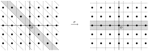
Figure 1: The shear transformation $\sigma$ (illustrated here for $M=2$) maps sheared cubes to cubes. The dots are the sites of the integer lattice $\mathbbm{Z}^{2}$. The gray band on the left encompasses those sheared cubes that intersect $S_{0}$.

Using the projection $\pi$, we now define a new measure $\mu_{0}$ on the Borel subsets of $\mathbbm{R}^{M}$, which is concentrated on $S_{0}$, by

$$\mu_{0}(\,\cdot\,):=\lambda^{M-1}(\pi(\,\cdot\,\cap S_{0})),$$

where $\lambda^{M-1}$ is the ordinary Lebesgue measure on $\mathbbm{R}^{M-1}$. Note that up to a multiplicative constant, $\mu_{0}$ is equal to the measure $\nu_{0}$ defined in Section 3, so we could have stated Theorems 1.4 and 1.5 equally well with $\mu_{0}$ instead of $\nu_{0}$. In the proofs it turns out to be more convenient to work with $\mu_{0}$, however, so that is what we shall do.

Our proofs of Theorems 1.4 and 1.5 resemble classical arguments to prove weak convergence of random vectors living on a lattice via a local limit theorem and Scheffé’s theorem, see for instance [1, Theorem 3.3]. However, we cannot use these classic results here, for two reasons. First of all, in Theorem 1.5 our random vectors live on an $M$-dimensional lattice, but in the limit all the mass collapses onto a lower-dimensional hyperplane, leading to a weak limit which is singular with respect to $M$-dimensional Lebesgue measure. The classic arguments do not cover this case of a singular limit.

Secondly, we are considering conditioned random vectors, for which it is not so obvious how to obtain a local limit theorem directly. Our solution is to get rid of the conditioning by considering ratios of conditioned probabilities, and prove a local limit theorem for these ratios. An extra argument will then be needed to prove weak convergence. Since we cannot resort to classic arguments here, we have to go through the proofs in considerable detail.

3.1 Proof of Theorem 1.4

As we have explained above, the key idea in the proof of Theorem 1.4 is that we can get rid of the awkward conditioning by considering ratios of conditional probabilities, rather than the conditional probabilities themselves. Thus, we will be dealing with ratios of binomial probabilities, and the following lemma addresses the key properties of these ratios needed in the proof. The lemma resembles standard bounds on binomial probabilities, but we point out that here we are considering ratios of binomial probabilities which centre around $c_{in}m_{in}$ rather than around the mean $p_{i}m_{in}$. We also note that actually, the lemma is stronger than required to prove Theorem 1.4, but we will need this stronger result to prove Theorem 1.5 later.

Lemma 3.2.

Recall the definition (14) of $A_{n}$. Fix $i\in\{1,2,\dots,M\}$ and let $b_{1},b_{2},\dotsc$ be a sequence of positive integers such that $b_{n}/\sqrt{n}\to 0$ as $n\to\infty$. Then, for every $z\in\mathbbm{R}$,

$$\sup_{\begin{subarray}{c}x\colon\lvert x-x_{in}\rvert<b_{n}\\ r\colon\lvert r-z\sqrt{n}\rvert<b_{n}\end{subarray}}\left|\frac{1}{A_{n}^{r}}\frac{\mathop{\hbox{}\mathbbm{P}}(X_{in}=x+r)}{\mathop{\hbox{}\mathbbm{P}}(X_{in}=x)}-\exp\left(-\frac{z^{2}}{2c_{i}(1-c_{i})\alpha_{i}}\right)\right|\to 0.$$

Furthermore, there exist constants $B^{1}_{i},B^{2}_{i}<\infty$ such that for all $n$ and $r$,

$$\sup_{x\colon\lvert x-x_{in}\rvert<b_{n}}\frac{1}{A_{n}^{r}}\frac{\mathop{\hbox{}\mathbbm{P}}(X_{in}=x+r)}{\mathop{\hbox{}\mathbbm{P}}(X_{in}=x)}\leq B^{1}_{i}\left(1+\frac{r^{4}}{n^{2}}\right)\exp\left(B^{2}_{i}\frac{\lvert r\rvert}{\sqrt{n}}-\frac{1}{2}\frac{r^{2}}{n}\right).$$

Proof.

Robbins’ note on Stirling’s formula [5] states that for all $m=1,2,\dotsc$,

$$\sqrt{2\pi}\,m^{m+1/2}\,e^{-m+1/(12m+1)}<m!<\sqrt{2\pi}\,m^{m+1/2}\,e^{-m+1/(12m)},$$

from which it is straightforward to show that for all $m=0,1,2,\dotsc$ (so including $m=0$), there exists an $\eta_{m}$ satisfying $1/7<\eta_{m}<1/5$ such that

$$m!=\sqrt{2\pi(m+\eta_{m})}\,m^{m}\,e^{-m}=\sqrt{2\pi\mathopen{[\![}m\mathclose{]\!]}}\,m^{m}\,e^{-m},$$ (18)

where we have introduced the notation $\mathopen{[\![}m\mathclose{]\!]}:=m+\eta_{m}$.

Since $X_{in}$ has the binomial distribution with parameters $m_{in}$ and $p_{i}$,

$$\frac{1}{A_{n}^{r}}\frac{\mathop{\hbox{}\mathbbm{P}}(X_{in}=x+r)}{\mathop{\hbox{}\mathbbm{P}}(X_{in}=x)}=\frac{x!}{(x+r)!}\,\frac{(m_{in}-x)!}{(m_{in}-x-r)!}\left(\frac{c_{in}}{1-c_{in}}\right)^{r}.$$

Using (18), we can write this as the product of the three factors

$$P^{1}_{in}(x,r) =\left(\frac{\mathopen{[\![}x\mathclose{]\!]}}{\mathopen{[\![}x+r\mathclose{]\!]}}\>\frac{\mathopen{[\![}m_{in}-x\mathclose{]\!]}}{\mathopen{[\![}m_{in}-x-r\mathclose{]\!]}}\right)^{1/2}$$

$$P^{2}_{in}(x,r) =\left(\frac{c_{in}m_{in}}{x}\frac{m_{in}-x}{m_{in}-c_{in}m_{in}}\right)^{r}$$

$$P^{3}_{in}(x,r) =\left(\frac{x}{x+r}\right)^{x+r}\!\!\left(\frac{m_{in}-x}{m_{in}-x-r}\right)^{m_{in}-x-r}$$

for all $x$ and $r$ such that $0<x<m_{in}$ and $0\leq x+r\leq m_{in}$.

To study the convergence of $P^{3}_{in}(x,r)$, first write

$$P^{3}_{in}(x,r)=\left(1-\frac{r}{x+r}\right)^{x+r}\!\!\left(1+\frac{r}{m_{in}-x-r}\right)^{m_{in}-x-r}.$$

Using the fact that for all $u>-1$, $(1+u)$ lies between $\exp\bigl{(}u-\tfrac{1}{2}u^{2}\bigr{)}$ and $\exp\bigl{(}u-\tfrac{1}{2}u^{2}/(1+u)\bigr{)}$, a little computation now shows that $P^{3}_{in}(x,r)$ is wedged in between

$$\exp\left(-\frac{1}{2}\frac{(m_{in}-r)r^{2}}{x(m_{in}-x-r)}\right)\quad\text{and}\quad\exp\left(-\frac{1}{2}\frac{(m_{in}+r)r^{2}}{(x+r)(m_{in}-x)}\right).$$

From this fact, it follows that for fixed $z\in\mathbbm{R}$,

$$\sup_{\begin{subarray}{c}x\colon\lvert x-x_{in}\rvert<b_{n}\\ r\colon\lvert r-z\sqrt{n}\rvert<b_{n}\end{subarray}}\left|P^{3}_{in}(x,r)-\exp\left(-\frac{z^{2}}{2c_{i}(1-c_{i})\alpha_{i}}\right)\right|\to 0,$$

because $x_{in}/m_{in}\to c_{i}$, hence $x=c_{i}m_{in}+o(n)$ and $r=z\sqrt{n}+o(\sqrt{n})$ under the supremum, and $m_{in}/n\to\alpha_{i}$. Since $\lvert x_{in}-c_{in}m_{in}\rvert<1$, we also have that

$$\sup_{\begin{subarray}{c}x\colon\lvert x-x_{in}\rvert<b_{n}\\ r\colon\lvert r-z\sqrt{n}\rvert<b_{n}\end{subarray}}\left|P^{1}_{in}(x,r)-1\right|\to 0\quad\text{and}\quad\sup_{\begin{subarray}{c}x\colon\lvert x-x_{in}\rvert<b_{n}\\ r\colon\lvert r-z\sqrt{n}\rvert<b_{n}\end{subarray}}\left|P^{2}_{in}(x,r)-1\right|\to 0.$$

Together with the uniform convergence of $P^{3}_{in}(x,r)$, this establishes the first part of Lemma 3.2.

We now turn to the second part of the lemma. If $x$ and $r$ are such that $0<x<m_{in}$ and $0\leq x+r\leq m_{in}$, then $m_{in}-r\geq x>0$ and $m_{in}+r\geq m_{in}-x>0$, hence from the bounds on $P^{3}_{in}(x,r)$ given in the previous paragraph we can conclude that

$$P^{3}_{in}(x,r)\leq\exp\left(-\frac{1}{2}\frac{r^{2}}{m_{in}}\right)\leq\exp\left(-\frac{1}{2}\frac{r^{2}}{n}\right).$$

Next observe that if $x$ is such that $\lvert x-x_{in}\rvert<b_{n}$, then $\lvert x-c_{in}m_{in}\rvert<1+b_{n}$, from which it follows that uniformly in $n$, for all $x$ and $r$ such that $0<x<m_{in}$, $0\leq x+r\leq m_{in}$ and $\lvert x-x_{in}\rvert<b_{n}$,

$$P^{2}_{in}(x,r)\leq\left(1+\text{const.}\times\frac{b_{n}}{n}\right)^{\lvert r\rvert}\leq\exp\left(\text{const.}\times\frac{\lvert r\rvert}{\sqrt{n}}\right).$$

To finish the proof, it remains to bound $P^{1}_{in}(x,r)$. To this end, observe first that uniformly in $n$, for all $x$ and $r$ such that $\lvert x-x_{in}\rvert<b_{n}$ and $\lvert r\rvert<n^{3/4}$, $P^{1}_{in}(x,r)$ is bounded by a constant. On the other hand, uniformly for all $x$ and $r$ such that $0<x<m_{in}$ and $0\leq x+r\leq m_{in}$, $P^{1}_{in}(x,r)$ is bounded by a constant times $n$, and $n\leq r^{4}/n^{2}$ if $\lvert r\rvert\geq n^{3/4}$. Combining these observations, we see that uniformly in $n$, for all $x$ and $r$ satisfying $\lvert x-x_{in}\rvert<b_{n}$ and $0\leq x+r\leq m_{in}$,

$$P^{1}_{in}(x,r)\leq\text{const.}\times\left(1+\frac{r^{4}}{n^{2}}\right).\qed$$

Proof of Theorem 1.4.

For a point $z$ in $\mathbbm{R}^{M}$, let $\lceil z\rfloor$ be the point in $\mathbbm{Z}^{M}$ $\rho$-closest to $z$ (take the lexicographically smallest one if there is a choice). Graphically, this means that the collection of those points $z$ for which $\lceil z\rfloor=a$ comprises the sheared cube $a+\sigma^{-1}(-1/2,1/2]^{M}$, see Figure 1. Now, for each fixed $z\in\mathbbm{R}^{M}$, set $r^{z}_{n}=(r^{z}_{1n},\dots,r^{z}_{Mn}):=\lceil z\sqrt{n}\rfloor$. Observe that because (for fixed $n$) the $x_{in}$ sum to $k_{n}$, if $r^{z}_{n}\in S_{0}$ we have that

$$\frac{\mathop{\hbox{}\mathbbm{P}}(\sqrt{n}\,\bm{\mathcal{X}}_{n}=r^{z}_{n}\mid\Sigma_{n}=k_{n})}{\mathop{\hbox{}\mathbbm{P}}(\sqrt{n}\,\bm{\mathcal{X}}_{n}=0\mid\Sigma_{n}=k_{n})}=\frac{\mathop{\hbox{}\mathbbm{P}}(\sqrt{n}\,\bm{\mathcal{X}}_{n}=r^{z}_{n})}{\mathop{\hbox{}\mathbbm{P}}(\sqrt{n}\,\bm{\mathcal{X}}_{n}=0)}=\prod_{i=1}^{M}\frac{\mathop{\hbox{}\mathbbm{P}}(X_{in}=x_{in}+r^{z}_{in})}{\mathop{\hbox{}\mathbbm{P}}(X_{in}=x_{in})},$$ (19)

where we have used the independence of the components $X_{in}$. If $r^{z}_{n}\notin S_{0}$, on the other hand, this ratio obviously vanishes.

We now apply Lemma 3.2 to (19), taking $b_{n}=M$ for every $n\geq 1$. Since $\sum_{i=1}^{M}r^{z}_{in}=0$ if $r^{z}_{n}\in S_{0}$ and hence $\prod_{i=1}^{M}A_{n}^{r^{z}_{in}}=1$, the first part of Lemma 3.2 immediately implies that for all $z\in\mathbbm{R}^{M}$,

$$\frac{\mathop{\hbox{}\mathbbm{P}}(\sqrt{n}\,\bm{\mathcal{X}}_{n}=r^{z}_{n}\mid\Sigma_{n}=k_{n})}{\mathop{\hbox{}\mathbbm{P}}(\sqrt{n}\,\bm{\mathcal{X}}_{n}=0\mid\Sigma_{n}=k_{n})}\to\mathop{\hbox{}\mathbbm{1}}\nolimits_{S_{0}}(z)\prod_{i=1}^{M}\exp\left(-\frac{z_{i}^{2}}{2c_{i}(1-c_{i})\alpha_{i}}\right)=f(z)$$

as $n\to\infty$. To see how this will lead to Theorem 1.4, define $f_{n}\colon\mathbbm{R}^{M}\to\mathbbm{R}$ by

$$f_{n}(z):=(\sqrt{n})^{M}\mathop{\hbox{}\mathbbm{P}}\bigl{(}\sqrt{n}\,\bm{\mathcal{X}}_{n}=r^{z}_{n}\bigm{|}\Sigma_{n}=k_{n}\bigr{)}.$$

Then $f_{n}$ is a probability density function with respect to $M$-dimensional Lebesgue measure $\lambda$. Moreover, if $\bm{\mathcal{Z}}_{n}$ is a random vector with this density, then the vector $\bm{\mathcal{Z}}^{\prime}_{n}=\lceil\bm{\mathcal{Z}}_{n}\sqrt{n}\rfloor/\sqrt{n}$ has the same distribution as the vector $\bm{\mathcal{X}}_{n}$, conditioned on $\{\Sigma_{n}=k_{n}\}$. Since clearly $\bm{\mathcal{Z}}_{n}$ and $\bm{\mathcal{Z}}^{\prime}_{n}$ must have the same weak limit, it is therefore sufficient to show that the weak limit of $\bm{\mathcal{Z}}_{n}$ has density $f/\int f\,d\mu_{0}$ with respect to $\mu_{0}$.

Now, by what we have established above, we already know that

$$\frac{f_{n}(z)}{f_{n}(0)}=\frac{\mathop{\hbox{}\mathbbm{P}}(\sqrt{n}\,\bm{\mathcal{X}}_{n}=r^{z}_{n}\mid\Sigma_{n}=k_{n})}{\mathop{\hbox{}\mathbbm{P}}(\sqrt{n}\,\bm{\mathcal{X}}_{n}=0\mid\Sigma_{n}=k_{n})}\to f(z)\qquad\text{for every $z\in\mathbbm{R}^{M}$}.$$

Moreover, the second part of Lemma 3.2 applied to (19) shows that the ratios $f_{n}(z)/f_{n}(0)$ are uniformly bounded by some $\mu_{0}$-integrable function $g(z)$. Thus it follows by dominated convergence that for every Borel set $A\subset\mathbbm{R}^{M}$,

$$\int_{A}\frac{f_{n}(z)}{f_{n}(0)}\,d\mu_{0}(z)\to\int_{A}f(z)\,d\mu_{0}(z).$$

Next observe that $1=\int f_{n}\,d\lambda=\int n^{-1/2}f_{n}\,d\mu_{0}$, because by the conditioning, $f_{n}$ is nonzero only on the sheared cubes which intersect $S_{0}$. Therefore, taking $A=\mathbbm{R}^{M}$ in the previous equation yields $n^{-1/2}f_{n}(0)\to(\int f\,d\mu_{0})^{-1}$, which in turn implies that for every Borel set $A$,

$$\int_{A}n^{-1/2}f_{n}(z)\,d\mu_{0}(z)\to\frac{\int_{A}f(z)\,d\mu_{0}(z)}{\int f\,d\mu_{0}}.$$

In general, $\int_{F}f_{n}\,d\lambda\neq\int_{F}n^{-1/2}f_{n}\,d\mu_{0}$ for an arbitrary Borel set $F$, but we have equality here for sufficiently large $n$ if $F$ is a finite union of sheared cubes. Hence, if $A$ is open, we can approximate $A$ from the inside by unions of sheared cubes contained in $A$ to conclude that

$$\liminf_{n\to\infty}\int_{A}f_{n}(z)\,d\lambda(z)\geq\frac{\int_{A}f(z)\,d\mu_{0}(z)}{\int f\,d\mu_{0}}.\qed$$

3.2 Proof of Theorem 1.5

We now turn to the case where we condition on $\{\Sigma_{n}\geq k_{n}\}$, for the same fixed sequence $k_{n}\to\infty$ as before. To treat this case, we are going to consider what happens when we condition on the event that $\Sigma_{n}=k_{n}+\ell$ for some $\ell\geq 0$, and later sum over $\ell$. It will be important for us to know the relevant range of $\ell$ to sum over. In particular, for large enough $\ell$ we expect that the probability $\mathop{\hbox{}\mathbbm{P}}(\Sigma_{n}=k_{n}+\ell)$ will be so small, that these $\ell$ will not influence the conditional distribution of the vector $\bm{\mathcal{X}}_{n}$ in an essential way. The relevant range of $\ell$ can be determined from the following lemma:

Lemma 3.3.

For all positive integers $s$,

$$\mathop{\hbox{}\mathbbm{P}}(\Sigma_{n}\geq k_{n}+2Ms)\leq M\exp\left(-\frac{(k_{n}-\mathop{\hbox{}\mathbbm{E}}(\Sigma_{n})+Ms)s}{Mn}\right)\mathop{\hbox{}\mathbbm{P}}(\Sigma_{n}\geq k_{n}).$$

Proof.

Let $u$ be such that $0<u<(1-p_{i})m_{in}$. Observe that then, for all integers $m$ such that $p_{i}m_{in}+u\leq m\leq m_{in}$,

$$\frac{\mathop{\hbox{}\mathbbm{P}}(X_{in}=m+1)}{\mathop{\hbox{}\mathbbm{P}}(X_{in}=m)}=\frac{m_{in}-m}{m+1}\frac{p_{i}}{1-p_{i}}\leq\frac{p_{i}m_{in}-u\frac{p_{i}}{1-p_{i}}}{p_{i}m_{in}+u},$$

hence

$$\frac{\mathop{\hbox{}\mathbbm{P}}(X_{in}=m+1)}{\mathop{\hbox{}\mathbbm{P}}(X_{in}=m)}\leq 1-\frac{u}{p_{i}m_{in}+u}\left(1+\frac{p_{i}}{1-p_{i}}\right)\leq 1-\frac{u}{m_{in}}\leq 1-\frac{u}{n}.$$

Since $1-z\leq\exp(-z)$, by repeated application of this inequality it follows that for all $u>0$ and all positive integers $t$, if $m$ is an integer such that $m\geq p_{i}m_{in}+u$, then

$$\mathop{\hbox{}\mathbbm{P}}(X_{in}=m+t)\leq\exp\left(-\frac{ut}{n}\right)\mathop{\hbox{}\mathbbm{P}}(X_{in}=m).$$ (20)

Now observe that if $\Sigma_{n}\geq\mathop{\hbox{}\mathbbm{E}}(\Sigma_{n})+Mr+2Ms$, where $s$ is a positive integer, and $r$ a real number such that $r+s>0$, then for some $k$ it must be the case that $X_{kn}\geq p_{k}m_{kn}+r+2s$. Therefore,

$$\mathop{\hbox{}\mathbbm{P}}(\Sigma_{n}\geq\mathop{\hbox{}\mathbbm{E}}(\Sigma_{n})+Mr+2Ms)\\ \leq\sum_{\begin{subarray}{c}\ell_{1},\dots,\ell_{M}\in\mathbbm{N}_{0}\colon\\ \ell_{1}+\dots+\ell_{M}\geq\mathop{\hbox{}\mathbbm{E}}(\Sigma_{n})+Mr+2Ms\end{subarray}}\sum_{k=1}^{M}\mathop{\hbox{}\mathbbm{1}}\nolimits(\ell_{k}\geq p_{k}m_{kn}+r+2s)\mathop{\hbox{}\mathbbm{P}}(X_{in}=\ell_{i}\ \forall i).$$

But by (20), taking $u=r+s$ and $t=s$,

$$\mathop{\hbox{}\mathbbm{1}}\nolimits(\ell_{k}\geq p_{k}m_{kn}+r+2s)\mathop{\hbox{}\mathbbm{P}}(X_{in}=\ell_{i}\ \forall i)\\ \leq\exp\left(-\frac{(r+s)s}{n}\right)\mathop{\hbox{}\mathbbm{P}}(X_{kn}=\ell_{k}-s,X_{in}=\ell_{i}\ \forall i\neq k),$$

and therefore

$$\mathop{\hbox{}\mathbbm{P}}(\Sigma_{n}\geq\mathop{\hbox{}\mathbbm{E}}(\Sigma_{n})+Mr+2Ms)\\ \begin{aligned} &\leq M\exp\left(-\frac{(r+s)s}{n}\right)\mathop{\hbox{}\mathbbm{P}}(\Sigma_{n}\geq\mathop{\hbox{}\mathbbm{E}}(\Sigma_{n})+Mr+2Ms-s)\\ &\leq M\exp\left(-\frac{(r+s)s}{n}\right)\mathop{\hbox{}\mathbbm{P}}(\Sigma_{n}\geq\mathop{\hbox{}\mathbbm{E}}(\Sigma_{n})+Mr\bigr{)}.\end{aligned}$$

Choosing $r$ such that $k_{n}\equiv\mathop{\hbox{}\mathbbm{E}}(\Sigma_{n})+Mr$ yields Lemma 3.3 (observe that the bound holds trivially if $r+s\leq 0$). ∎

Lemma 3.3 shows that if $\alpha>\sum_{i=1}^{M}p_{i}\alpha_{i}$, then for sufficiently large $n$, $\mathop{\hbox{}\mathbbm{P}}(\Sigma_{n}\geq k_{n}+\ell)$ will already be much smaller than $\mathop{\hbox{}\mathbbm{P}}(\Sigma_{n}\geq k_{n})$ when $\ell$ is of order $\log n$. However, when $\alpha=\sum_{i=1}^{M}p_{i}\alpha_{i}$, we need to consider $\ell$ of bigger order than $\sqrt{n}$ for $\mathop{\hbox{}\mathbbm{P}}(\Sigma_{n}\geq k_{n}+\ell)$ to become much smaller than $\mathop{\hbox{}\mathbbm{P}}(\Sigma_{n}\geq k_{n})$. In either case, Lemma 3.3 shows that $\ell$ of larger order than $\sqrt{n}$ become irrelevant.

Keeping this in mind, we will now look at the conditional distribution of the vector $\bm{\mathcal{X}}_{n}$, conditioned on $\{\Sigma_{n}=k_{n}+\ell\}$. The first thing to observe is that for $\ell>0$, the locations of the centres around which the components $X_{in}$ concentrate will be shifted to larger values. Indeed, these centres are located at $c^{\ell}_{in}m_{in}$, where the $c^{\ell}_{in}$ are of course determined by the system of equations

$$\left\{\begin{aligned} &\frac{1-c^{\ell}_{in}}{c^{\ell}_{in}}\frac{p_{i}}{1-p_{i}}=\frac{1-c^{\ell}_{jn}}{c^{\ell}_{jn}}\frac{p_{j}}{1-p_{j}}&&&\forall i,j\in\{1,\dots,M\};\\ &\textstyle\sum_{i=1}^{M}c^{\ell}_{in}m_{in}=k_{n}+\ell.\end{aligned}\right.$$ (21)

To find an explicit expression for the size of the shift $c^{\ell}_{in}-c_{in}$, we can substitute $c^{\ell}_{in}=c_{in}+\delta_{in}$ into (21), and then perform an expansion in powers of the correction $\delta_{in}$ to guess this correction to first order. This procedure leads us to believe that $c^{\ell}_{in}$ must be of the form

$$c^{\ell}_{in}=c_{in}+c_{in}(1-c_{in})d^{\ell}_{n}+e^{\ell}_{in},$$ (22)

where

$$d^{\ell}_{n}:=\frac{\ell}{\sum_{j=1}^{M}c_{jn}(1-c_{jn})m_{jn}},$$

and $e^{\ell}_{in}$ should be a higher-order correction. The following lemma shows that the error terms $e^{\ell}_{in}$ are indeed of second order in $d^{\ell}_{n}$, so that the effective shift in $c_{in}$ by adding $\ell$ extra successes to our Bernoulli variables is given by $c_{in}(1-c_{in})d^{\ell}_{n}$. For convenience, we assume in the lemma that $\lvert d^{\ell}_{n}\rvert\leq 1/2$, which means that $\lvert\ell\rvert$ cannot be too large, but by Lemma 3.3, this does not put too severe a restriction on the range of $\ell$ we can consider later.

Lemma 3.4.

For all $\ell$ (positive or negative) such that $\lvert d^{\ell}_{n}\rvert\leq 1/2$, we have that $\lvert e^{\ell}_{in}\rvert\leq(d^{\ell}_{n})^{2}$ for all $i=1,\dots,M$.

Proof.

For ease of notation, write $\sigma_{in}:=c_{in}(1-c_{in})$. As before, we write

$$A^{\ell}_{n}=\frac{1-c^{\ell}_{in}}{c^{\ell}_{in}}\frac{p_{i}}{1-p_{i}}=\frac{1-c_{in}-\sigma_{in}d^{\ell}_{n}-e^{\ell}_{in}}{c_{in}+\sigma_{in}d^{\ell}_{n}+e^{\ell}_{in}}\frac{p_{i}}{1-p_{i}}$$

for the desired common value for all $i$, so

$$e^{\ell}_{in}=\frac{p_{i}(1-c_{in}-\sigma_{in}d^{\ell}_{n})-A^{\ell}_{n}(1-p_{i})(c_{in}+\sigma_{in}d^{\ell}_{n})}{A^{\ell}_{n}(1-p_{i})+p_{i}}.$$ (23)

As before, the value of $A^{\ell}_{n}$ is uniquely determined by the requirement that $\sum_{i=1}^{M}c^{\ell}_{in}m_{in}=k_{n}+\ell$. Since $\sum_{i=1}^{M}c_{in}m_{in}=k_{n}$ and $\sum_{i=1}^{M}\sigma_{in}d^{\ell}_{n}m_{in}=\ell$, this requirement says that

$$\sum_{i=1}^{M}e^{\ell}_{in}m_{in}=0.$$

In particular, the $e^{\ell}_{in}$ cannot be all positive or all negative, from which we derive, using (23), that $A^{\ell}_{n}$ must satisfy the double inequalities

$$\min_{i=1,\dots,M}\left\{\frac{p_{i}(1-c_{in}-\sigma_{in}d^{\ell}_{n})}{(1-p_{i})(c_{in}+\sigma_{in}d^{\ell}_{n})}\right\}\leq A^{\ell}_{n}\leq\max_{i=1,\dots,M}\left\{\frac{p_{i}(1-c_{in}-\sigma_{in}d^{\ell}_{n})}{(1-p_{i})(c_{in}+\sigma_{in}d^{\ell}_{n})}\right\}.$$

A simple calculation establishes that

$$\frac{p_{i}(1-c_{in}-\sigma_{in}d^{\ell}_{n})}{(1-p_{i})(c_{in}+\sigma_{in}d^{\ell}_{n})}=\frac{1-c_{in}}{c_{in}}\frac{p_{i}}{1-p_{i}}\left(1+\sum_{k=1}^{\infty}\frac{(-(1-c_{in})d^{\ell}_{n})^{k}}{1-c_{in}}\right),$$

from which (using $\lvert d^{\ell}_{n}\rvert\leq 1/2$) we can conclude that

$$\frac{1-c_{in}}{c_{in}}\frac{p_{i}}{1-p_{i}}\bigl{(}1-d^{\ell}_{n}\bigr{)}\leq A^{\ell}_{n}\leq\frac{1-c_{in}}{c_{in}}\frac{p_{i}}{1-p_{i}}(1-d^{\ell}_{n}+2\bigl{(}d^{\ell}_{n})^{2}\bigr{)},$$

since by (3), neither the lower bound nor the upper bound here depends on $i$.

Inserting the lower bound on $A^{\ell}_{n}$ into (23) gives

$$e^{\ell}_{in}\leq\frac{\sigma_{in}(1-c_{in})(d^{\ell}_{n})^{2}}{1-(1-c_{in})d^{\ell}_{n}}\leq\frac{1}{2}(d^{\ell}_{n})^{2},$$

where in the last step we used that $\lvert d^{\ell}_{n}\rvert\leq 1/2$ and $\sigma_{in}\leq 1/4$. Likewise, substituting the upper bound on $A^{\ell}_{n}$ into (23) yields

$$e^{\ell}_{in}\geq-\frac{\sigma_{in}(1+c_{in})(d^{\ell}_{n})^{2}+2\sigma_{in}(1-c_{in})(d^{\ell}_{n})^{3}}{1-(1-c_{in})d^{\ell}_{n}+2(1-c_{in})(d^{\ell}_{n})^{2}}\geq-\frac{2\sigma_{in}(d^{\ell}_{n})^{2}}{1-1/2}\geq-(d^{\ell}_{n})^{2}.\qed$$

For future use, we state the following corollary:

Corollary 3.5.

If $(k_{n}-\sum_{i=1}^{M}c_{i}m_{in})/\sqrt{n}\to K$ for some $K\in[-\infty,\infty]$, then for $i\in\{1,\dots,M\}$,

$$\frac{(c_{in}-c_{i})m_{in}}{\sqrt{n}}\to\frac{c_{i}(1-c_{i})\alpha_{i}}{\sum_{j=1}^{M}c_{j}(1-c_{j})\alpha_{j}}K.$$

Remark 3.6.

If $(k_{n}-\mathop{\hbox{}\mathbbm{E}}(\Sigma_{n}))/\sqrt{n}\to K\in\mathbbm{R}$, then $\alpha=\sum_{i=1}^{M}p_{i}\alpha_{i}$ and we have $c_{i}=p_{i}$ for all $i\in\{1,\dots,M\}$. In this situation, Corollary 3.5 states that the vectors $\bm{\mathcal{X}}^{p}_{n}-\bm{\mathcal{X}}_{n}$, and hence also the same vectors conditioned on $\{\Sigma_{n}\geq k_{n}\}$, converge pointwise to the vector whose $i$-th component is

$$\frac{p_{i}(1-p_{i})\alpha_{i}}{\sum_{j=1}^{M}p_{j}(1-p_{j})\alpha_{j}}K.$$

Proof of Corollary 3.5.

First, suppose that $K\in\mathbbm{R}$. If $\ell=\sum_{i=1}^{M}c_{i}m_{in}-k_{n}$ and the $c_{in}^{\ell}$ satisfy (21), then $c_{in}^{\ell}=c_{i}$. Hence, by Lemma 3.4,

$$c_{i}-c_{in}=c_{in}(1-c_{in})d_{n}^{\ell}+O\bigl{(}(d_{n}^{\ell})^{2}\bigr{)},$$

where

$$d_{n}^{\ell}=\frac{\sum_{i=1}^{M}c_{i}m_{in}-k_{n}}{\sum_{j=1}^{M}c_{jn}(1-c_{jn})m_{jn}}=O\bigl{(}n^{-1/2}\bigr{)}.$$

This implies

$$\frac{(c_{i}-c_{in})m_{in}}{\sqrt{n}}=\frac{c_{in}(1-c_{in})m_{in}}{\sum_{j=1}^{M}c_{jn}(1-c_{jn})m_{jn}}\frac{\sum_{i=1}^{M}c_{i}m_{in}-k_{n}}{\sqrt{n}}+O\bigl{(}n^{-1/2}\bigr{)},$$

from which the result follows.

Next, suppose that $K=\infty$. Since $c_{in}$ is increasing as a function of $k_{n}$, we have by the first part of the proof

$$\liminf_{n\to\infty}\frac{(c_{in}-c_{i})m_{in}}{\sqrt{n}}\geq\frac{c_{i}(1-c_{i})\alpha_{i}}{\sum_{j=1}^{M}c_{j}(1-c_{j})\alpha_{j}}L$$

for all $L\in\mathbbm{R}$. Hence, the left-hand side is equal to $\infty$. The proof for the case $K=-\infty$ is similar. ∎

When we condition on $\{\Sigma_{n}=k_{n}+\ell\}$, then in analogy with what we have done before, the natural scaled vector to consider would be the vector

$$\bm{\mathcal{X}}^{\ell}_{n}:=\left(\frac{X_{1n}-x^{\ell}_{1n}}{\sqrt{n}},\frac{X_{2n}-x^{\ell}_{2n}}{\sqrt{n}},\dots,\frac{X_{Mn}-x^{\ell}_{Mn}}{\sqrt{n}}\right),$$

where the components of the vector $x^{\ell}_{n}=(x^{\ell}_{1n},\dots,x^{\ell}_{Mn})$ identify the centres around which the $X_{in}$ concentrate. Here, the $x^{\ell}_{in}$ are nonnegative integers chosen such that $\lvert x^{\ell}_{in}-c^{\ell}_{in}m_{in}\rvert<1$ for all $i$, and $\sum_{i=1}^{M}x^{\ell}_{in}=k_{n}+\ell$. Note that the vector $\bm{\mathcal{X}}^{\ell}_{n}$ is simply a translation of $\bm{\mathcal{X}}_{n}$ by $(x^{\ell}_{n}-x_{n})/\sqrt{n}$. Since Lemma 3.3 shows that if $k_{n}$ is sufficiently larger than $\mathop{\hbox{}\mathbbm{E}}(\Sigma_{n})$, only values of $\ell$ up to small order in $n$ are relevant, the statement of Theorem 1.5 should not come as a surprise. To prove it, we need to refine the arguments we used to prove Theorem 1.4.

Proof of Theorem 1.5.

Assume that $(k_{n}-\mathop{\hbox{}\mathbbm{E}}(\Sigma_{n}))/\sqrt{n}\to\infty$, and let

$$a_{n}:=2M\left\lfloor\sqrt{n}\left(\frac{\sqrt{n}}{k_{n}-\mathop{\hbox{}\mathbbm{E}}(\Sigma_{n})}\right)^{1/2}\right\rfloor.$$

Note that then $a_{n}\to\infty$ but $a_{n}/\sqrt{n}\to 0$. Furthermore, Lemma 3.3 and a short computation show that

$$\frac{\mathop{\hbox{}\mathbbm{P}}(\Sigma_{n}>k_{n}+a_{n})}{\mathop{\hbox{}\mathbbm{P}}(\Sigma_{n}\geq k_{n})}\to 0.$$

It is easy to see that from this last fact it follows that

$$\sup_{A}\Bigl{|}\mathop{\hbox{}\mathbbm{P}}(\bm{\mathcal{X}}_{n}\in A\mid\Sigma_{n}\geq k_{n})-\mathop{\hbox{}\mathbbm{P}}(\bm{\mathcal{X}}_{n}\in A\mid k_{n}\leq\Sigma_{n}\leq k_{n}+a_{n})\Bigr{|}\to 0,$$

where the supremum is over all Borel subsets $A$ of $\mathbbm{R}^{M}$. It is therefore sufficient to consider the limiting distribution of the vector $\bm{\mathcal{X}}_{n}$ conditioned on the event $\{k_{n}\leq\Sigma_{n}\leq k_{n}+a_{n}\}$, rather than on the event $\{\Sigma_{n}\geq k_{n}\}$.

As in the proof of Theorem 1.4, for $z\in\mathbbm{R}^{M}$ we let $r^{z}_{n}=\lceil z\sqrt{n}\rfloor$, and we define the functions $f_{n}\colon\mathbbm{R}^{M}\to\mathbbm{R}$ by setting

$$f_{n}(z):=(\sqrt{n})^{M}\mathop{\hbox{}\mathbbm{P}}\bigl{(}\sqrt{n}\,\bm{\mathcal{X}}_{n}=r^{z}_{n}\bigm{|}k_{n}\leq\Sigma_{n}\leq k_{n}+a_{n}\bigr{)}.$$

As before, this is a probability density function with respect to Lebesgue measure $\lambda$ on $\mathbbm{R}^{M}$, and if $\bm{\mathcal{Z}}_{n}$ is a random vector with this density, then the vector $\bm{\mathcal{Z}}_{n}^{\prime}=\lceil\bm{\mathcal{Z}}_{n}\sqrt{n}\rfloor/\sqrt{n}$ has the same distribution as the vector $\bm{\mathcal{X}}_{n}$ conditioned on the event $\{k_{n}\leq\Sigma_{n}\leq k_{n}+a_{n}\}$. Hence, it is enough to show that the weak limit of $\bm{\mathcal{Z}}_{n}$ has density $f/\int f\,d\mu_{0}$ with respect to $\mu_{0}$.

An essential difference compared to the situation in Theorem 1.4, however, is that the densities $f_{n}$ are no longer supported by the collection of points $z$ for which $r^{z}_{n}$ is in the hyperplane $S_{0}$ (i.e. the union of those sheared cubes that intersect $S_{0}$). Rather, the support now encompasses all the points $z$ for which $r^{z}_{n}$ is in any of the hyperplanes

$$S_{\ell}:=\{(z_{1},\dots,z_{M})\in\mathbbm{R}^{M}\colon z_{1}+\dots+z_{M}=\ell\},\qquad\ell=0,1,\dots,a_{n},$$

because if $r^{z}_{n}\in S_{\ell}$, then the event $\{\sqrt{n}\,\bm{\mathcal{X}}_{n}=r^{z}_{n}\}$ is contained in the event $\{\Sigma_{n}=k_{n}+\ell\}$. For this reason, the densities $f_{n}$ are not so convenient to work with here. Instead, it is more convenient to “coarse-grain” our densities by spreading the mass over sheared cubes of volume $((2a_{n}+1)/\sqrt{n})^{M}$ rather than volume $(1/\sqrt{n})^{M}$, to the effect that all the mass is again contained in the collection of sheared (coarse-grained) cubes intersecting $S_{0}$.

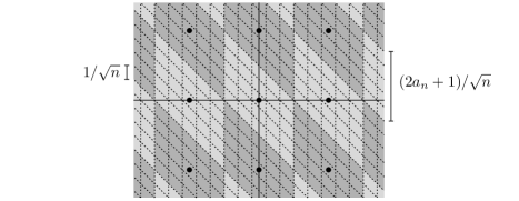
Figure 2: We coarse-grain our densities by combining $(2a_{n}+1)^{M}$ sheared cubes into larger sheared cubes. Here, we show this coarse-graining for $M=2$ and $a_{n}=2$. The dots are the points in $((2a_{n}+1)\mathbbm{Z})^{M}/\sqrt{n}$. The combined sheared cubes have been coloured in a chessboard fashion as a visual aid.

To this end, for given $n$ we partition $\mathbbm{R}^{M}$ into the collection of sets

$$\Bigl{\{}\frac{1}{\sqrt{n}}\bigl{(}a+\sigma^{-1}(-a_{n}-1/2,a_{n}+1/2]^{M}\bigr{)}\colon a\in\bigl{(}(2a_{n}+1)\mathbbm{Z}\bigr{)}^{M}\Bigr{\}}.$$ (24)

See Figure 2. For a given point $z\in\mathbbm{R}^{M}$, we denote by $Q_{n}^{z}$ the sheared cube in this partition containing $z$. Now we can define the coarse-grained densities

$$\begin{split}g_{n}(z)&:=\left(\frac{\sqrt{n}}{2a_{n}+1}\right)^{\!\!M}\mathop{\hbox{}\mathbbm{P}}(\bm{\mathcal{X}}_{n}\in Q^{z}_{n}\mid k_{n}\leq\Sigma_{n}\leq k_{n}+a_{n})\\ &\phantom{:}=\left(\frac{\sqrt{n}}{2a_{n}+1}\right)^{\!\!M}\int_{Q_{n}^{z}}f_{n}(y)\,d\lambda(y).\end{split}$$

By construction, these are again probability density functions with respect to $M$-dimensional Lebesgue measure $\lambda$. Moreover, each of these densities is supported on the collection of sheared cubes in (24) that intersect $S_{0}$, and is constant on each sheared cube $Q^{z}_{n}$. In particular, for any given point $z\in\mathbbm{R}^{M}$ we have

$$\int_{Q^{z}_{n}}g_{n}(y)\,d\lambda(y)=\frac{2a_{n}+1}{\sqrt{n}}\int_{Q^{z}_{n}}g_{n}(y)\,d\mu_{0}(y).$$

Finally, because $a_{n}/\sqrt{n}\to 0$ it is clear that if $\bm{\mathcal{Z}}_{n}^{\prime\prime}$ has density $g_{n}$, then its weak limit will coincide with that of $\bm{\mathcal{Z}}_{n}$, and hence also with that of the vector $\bm{\mathcal{X}}_{n}$ conditioned on the event $\{k_{n}\leq\Sigma_{n}\leq k_{n}+a_{n}\}$.

Suppose now that we could prove that

$$\frac{2a_{n}+1}{\sqrt{n}}g_{n}(z)\to\frac{f(z)}{\int f\,d\mu_{0}}\qquad\text{for every $z\in\mathbbm{R}^{M}$.}$$ (25)

Then it would follow from Fatou’s lemma that for every open set $A\subset\mathbbm{R}^{M}$,

$$\liminf_{n\to\infty}\int_{A}\frac{2a_{n}+1}{\sqrt{n}}g_{n}(z)\,d\mu_{0}(z)\geq\frac{\int_{A}f(z)\,d\mu_{0}(z)}{\int f\,d\mu_{0}}.$$

By approximating the open set $A$ by unions of sheared cubes contained in $A$, as in the proof of Theorem 1.4, it is then clear that this would imply that

$$\liminf_{n\to\infty}\int_{A}g_{n}(z)\,d\lambda(z)\geq\frac{\int_{A}f(z)\,d\mu_{0}(z)}{\int f\,d\mu_{0}}.$$

It therefore only remains to establish (25).

Since (25) holds by construction for $z\notin S_{0}$, we only need to consider the case $z\in S_{0}$. So let us fix $z\in S_{0}$, and look at $g_{n}(z)$. By definition, this is just the rescaled conditional probability that the vector $\bm{\mathcal{X}}_{n}$ lies in the sheared cube $Q^{z}_{n}$, given that $k_{n}\leq\Sigma_{n}\leq k_{n}+a_{n}$. In other words, if we define $C_{n}^{z}:=\sqrt{n}Q^{z}_{n}\cap\mathbbm{Z}^{M}$ and $C_{\ell n}^{z}:=C_{n}^{z}\cap S_{\ell}$, then we have

$$\begin{split}g_{n}(z)&=\left(\frac{\sqrt{n}}{2a_{n}+1}\right)^{\!\!M}\sum_{r\in C_{n}^{z}}\mathop{\hbox{}\mathbbm{P}}(\sqrt{n}\,\bm{\mathcal{X}}_{n}=r\mid k_{n}\leq\Sigma_{n}\leq k_{n}+a_{n})\\ &=\left(\frac{\sqrt{n}}{2a_{n}+1}\right)^{\!\!M}\sum_{\ell=0}^{a_{n}}\sum_{r\in C_{\ell n}^{z}}\frac{\mathop{\hbox{}\mathbbm{P}}(\sqrt{n}\,\bm{\mathcal{X}}_{n}=r\mid\Sigma_{n}=k_{n}+\ell)\mathop{\hbox{}\mathbbm{P}}(\Sigma_{n}=k_{n}+\ell)}{\mathop{\hbox{}\mathbbm{P}}(k_{n}\leq\Sigma_{n}\leq k_{n}+a_{n})}.\end{split}$$

Since $C^{z}_{\ell n}$ contains exactly $(2a_{n}+1)^{M-1}$ points, from this equality we conclude that to prove (25), it is sufficient to show that

$$\sup_{0\leq\ell\leq a_{n}}\sup_{r\in C^{z}_{\ell n}}\left|(\sqrt{n})^{M-1}\mathop{\hbox{}\mathbbm{P}}(\sqrt{n}\,\bm{\mathcal{X}}_{n}=r\mid\Sigma_{n}=k_{n}+\ell)-\frac{f(z)}{\int f\,d\mu_{0}}\right|\to 0.$$ (26)

The proof of (26) proceeds along the same line as the proof of pointwise convergence in Theorem 1.4, based on Lemma 3.2. However, there is a catch: because we are now conditioning on $\Sigma_{n}=k_{n}+\ell$, the $X_{in}$ are no longer centred around $x_{in}$, but around $x^{\ell}_{in}$. We therefore first write the conditional probabilities in a form analogous to what we had before, by using that

$$\mathop{\hbox{}\mathbbm{P}}\bigl{(}\sqrt{n}\,\bm{\mathcal{X}}_{n}=r\bigm{|}\Sigma_{n}=k_{n}+\ell\bigr{)}=\mathop{\hbox{}\mathbbm{P}}\bigl{(}\sqrt{n}\,\bm{\mathcal{X}}^{\ell}_{n}=r+x_{n}-x^{\ell}_{n}\bigm{|}\Sigma_{n}=k_{n}+\ell\bigr{)}.$$

Writing $r^{\ell}:=r+x_{n}-x^{\ell}_{n}$ for convenience, we now want to study the ratios

$$\frac{\mathop{\hbox{}\mathbbm{P}}(\sqrt{n}\,\bm{\mathcal{X}}^{\ell}_{n}=r^{\ell}\mid\Sigma_{n}=k_{n}+\ell)}{\mathop{\hbox{}\mathbbm{P}}(\sqrt{n}\,\bm{\mathcal{X}}^{\ell}_{n}=0\mid\Sigma_{n}=k_{n}+\ell)}=\frac{\mathop{\hbox{}\mathbbm{P}}(\sqrt{n}\,\bm{\mathcal{X}}^{\ell}_{n}=r^{\ell})}{\mathop{\hbox{}\mathbbm{P}}(\sqrt{n}\,\bm{\mathcal{X}}^{\ell}_{n}=0)}=\prod_{i=1}^{M}\frac{\mathop{\hbox{}\mathbbm{P}}(X_{in}=x^{\ell}_{in}+r^{\ell}_{i})}{\mathop{\hbox{}\mathbbm{P}}(X_{in}=x^{\ell}_{in})}$$

for $\ell$ and $r$ satisfying $0\leq\ell\leq a_{n}$ and $r\in C^{z}_{\ell n}$.

By equation (22) and Lemma 3.4 we have that $\sup_{\ell}\lvert x^{\ell}_{in}-x_{in}\rvert=o(\sqrt{n})$, from which it follows that also $\sup_{\ell,r}\lvert r^{\ell}-z\sqrt{n}\rvert=o(\sqrt{n})$, where the suprema are over all $\ell\in\{0,\dots,a_{n}\}$ and $r\in C^{z}_{\ell n}$. Thus, by the first part of Lemma 3.2,

$$\sup_{0\leq\ell\leq a_{n}}\sup_{r\in C^{z}_{\ell n}}\left|\frac{\mathop{\hbox{}\mathbbm{P}}(\sqrt{n}\,\bm{\mathcal{X}}^{\ell}_{n}=r^{\ell}\mid\Sigma_{n}=k_{n}+\ell)}{\mathop{\hbox{}\mathbbm{P}}(\sqrt{n}\,\bm{\mathcal{X}}^{\ell}_{n}=0\mid\Sigma_{n}=k_{n}+\ell)}-f(z)\right|\to 0,$$

where we have used that for all terms concerned, $\prod_{i=1}^{M}A_{n}^{r^{\ell}_{i}}=1$ because $r^{\ell}\in S_{0}$. Furthermore, from the second part of Lemma 3.2 it follows that the functions

$$z\mapsto\frac{\mathop{\hbox{}\mathbbm{P}}(\sqrt{n}\,\bm{\mathcal{X}}^{\ell}_{n}=\lceil z\sqrt{n}\rfloor\mid\Sigma_{n}=k_{n}+\ell)}{\mathop{\hbox{}\mathbbm{P}}(\sqrt{n}\,\bm{\mathcal{X}}^{\ell}_{n}=0\mid\Sigma_{n}=k_{n}+\ell)}$$

are bounded uniformly in $n$ and in all $\ell\in\{0,\dots,a_{n}\}$ by a $\mu_{0}$-integrable function. In the same way as in the proof of Theorem 1.4, it follows from these facts (with the addition that we have uniform bounds) that

$$\sup_{0\leq\ell\leq a_{n}}\left|(\sqrt{n})^{M-1}\mathop{\hbox{}\mathbbm{P}}(\sqrt{n}\,\bm{\mathcal{X}}^{\ell}_{n}=0\mid\Sigma_{n}=k_{n}+\ell)-\frac{1}{\int f\,d\mu_{0}}\right|\to 0.$$

From this we conclude that (26) does hold, which completes the proof of Theorem 1.5. ∎

3.3 Proof of Theorem 1.6

Proof of Theorem 1.6.

Suppose that $(k_{n}-\mathop{\hbox{}\mathbbm{E}}(\Sigma_{n}))/\sqrt{n}\to K$ for some $K\in[-\infty,\infty)$. Let $\bm{\mathcal{X}}$ be a random vector having a multivariate normal distribution with density $h/\int h\,d\lambda$ with respect to $\lambda$. By standard arguments, $\bm{\mathcal{X}}^{p}_{n}$ converges weakly to $\bm{\mathcal{X}}$. Therefore, for a rectangle $A\subset\mathbbm{R}^{M}$ we have

$$\mathop{\hbox{}\mathbbm{P}}(\bm{\mathcal{X}}^{p}_{n}\in A,\Sigma_{n}\geq k_{n})=\mathop{\hbox{}\mathbbm{P}}(\bm{\mathcal{X}}^{p}_{n}\in A\cap H_{\frac{k_{n}-\mathop{\hbox{}\mathbbm{E}}(\Sigma_{n})}{\sqrt{n}}})\to\mathop{\hbox{}\mathbbm{P}}(\bm{\mathcal{X}}\in A\cap H_{K}),$$

since $A\cap H_{K+\varepsilon}$ is a $\lambda$-continuity set for all $\varepsilon\in\mathbbm{R}$. Taking $A=\mathbbm{R}^{M}$ gives

$$\mathop{\hbox{}\mathbbm{P}}(\Sigma_{n}\geq k_{n})\to\mathop{\hbox{}\mathbbm{P}}(\bm{\mathcal{X}}\in H_{K}).$$

Hence, for all rectangles $A\subset\mathbbm{R}^{M}$

$$\mathop{\hbox{}\mathbbm{P}}(\bm{\mathcal{X}}^{p}_{n}\in A\mid\Sigma_{n}\geq k_{n})\to\frac{\mathop{\hbox{}\mathbbm{P}}(\bm{\mathcal{X}}\in A\cap H_{K})}{\mathop{\hbox{}\mathbbm{P}}(\bm{\mathcal{X}}\in H_{K})}.\qed$$

3.4 Law of large numbers

Finally, we prove a law of large numbers, which we will need in Section 4. Let $\tilde{X}_{in}$ denote a random variable with the conditional law of $X_{in}$, conditioned on the event $\{\Sigma_{n}\geq k_{n}\}$. If $(k_{n}-\mathop{\hbox{}\mathbbm{E}}(\Sigma_{n}))/\sqrt{n}\to K$ for some $K\in[-\infty,\infty]$, then an immediate consequence of Theorems 1.5 and 1.6 is that $\tilde{X}_{in}/n$ converges in probability to either $p_{i}\alpha_{i}$ or $c_{i}\alpha_{i}$. The following theorem shows that such a law of large numbers holds for a general sequence $k_{n}$ such that $k_{n}/n\to\alpha$.

Theorem 3.7.

For $i\in\{1,\dots,M\}$, the random variable $\tilde{X}_{in}/n$ converges in probability to $p_{i}\alpha_{i}$ if $\alpha\leq\sum_{i=1}^{M}p_{i}\alpha_{i}$, or to $c_{i}\alpha_{i}$ if $\alpha\geq\sum_{i=1}^{M}p_{i}\alpha_{i}$.

Proof.

If $\alpha\neq\sum_{i=1}^{M}p_{i}\alpha_{i}$, then $(k_{n}-\mathop{\hbox{}\mathbbm{E}}(\Sigma_{n}))/\sqrt{n}$ goes to $-\infty$ or $\infty$ as $n\to\infty$, and the result immediately follows from Theorem 1.5 and Theorem 1.6.

Now suppose that $\alpha=\sum_{i=1}^{M}p_{i}\alpha_{i}$. Then $c_{i}=p_{i}$ for all $i\in\{1,\dots,M\}$. Recall that in general the $c_{i}$ and $A$ are determined by the equations

$$c_{i}=\frac{p_{i}}{p_{i}+A(1-p_{i})}\quad\text{and}\quad\sum_{i=1}^{M}\frac{p_{i}\alpha_{i}}{p_{i}+A(1-p_{i})}=\alpha.$$

The constant $A$ is continuous as a function of $\alpha$, hence $c_{i}=c_{i}[\alpha]$ is also continuous as a function of $\alpha$. Therefore, if $\alpha=\sum_{i=1}^{M}p_{i}\alpha_{i}$, then for each $\varepsilon>0$ we can choose $\delta>0$ such that $c_{i}[\alpha+\delta]\alpha_{i}\leq p_{i}\alpha_{i}+\frac{1}{2}\varepsilon$. By Corollary 2.3 we have, for large enough $n$,

$$\mathop{\hbox{}\mathbbm{P}}(X_{in}\geq(p_{i}\alpha_{i}+\varepsilon)n\mid\Sigma_{n}\geq k_{n})\\ \begin{aligned} &\leq\mathop{\hbox{}\mathbbm{P}}(X_{in}\geq(p_{i}\alpha_{i}+\varepsilon)n\mid\Sigma_{n}\geq(\alpha+\delta)n)\\ &\leq\mathop{\hbox{}\mathbbm{P}}(X_{in}\geq(c_{i}[\alpha+\delta]\alpha_{i}+\tfrac{1}{2}\varepsilon)n\mid\Sigma_{n}\geq(\alpha+\delta)n),\end{aligned}$$

which tends to $0$ as $n\to\infty$ by Theorem 1.5. Similarly, using Corollary 2.3 and Theorem 1.6 instead of Theorem 1.5, we obtain

$$\mathop{\hbox{}\mathbbm{P}}(X_{in}\leq(p_{i}\alpha_{i}-\varepsilon)n\mid\Sigma_{n}\geq k_{n})\to 0.$$

We conclude that $\tilde{X}_{in}/n$ converges in probability to $p_{i}\alpha_{i}=c_{i}\alpha_{i}$. ∎

4 Asymptotic stochastic domination

4.1 Proof of Theorem 1.8

Consider the general framework for vectors $\bm{X}_{n}$ and $\bm{Y}_{n}$ of Section 1.2 in the setting of Section 1.4. We will split the proof of Theorem 1.8 into four lemmas. In the statements of these lemmas, we will need the constant $\hat{\alpha}$, which is defined as the limit as $n\to\infty$ of $\hat{k}_{n}/n$:

$$\hat{k}_{n}=\sum_{i=1}^{M}\frac{p_{i}m_{in}}{p_{i}+\beta_{\max}(1-p_{i})}\,,\quad\text{hence}\quad\hat{\alpha}=\sum_{i=1}^{M}\frac{p_{i}\alpha_{i}}{p_{i}+\beta_{\max}(1-p_{i})}\,.$$

Let us first look at the definition of $\hat{\alpha}$ in more detail. In Section 1.4, we informally introduced the sequence $\hat{k}_{n}$ as a critical sequence such that if $k_{n}$ is around $\hat{k}_{n}$, then there exists a block $i$ such that the number of successes $\tilde{X}_{in}$ of the vector $\tilde{\bm{X}}_{n}$ in block $i$ is roughly the same as $\tilde{Y}_{in}$. We will now make this precise. Recall that the $c_{i}$ and the constant $A$ are determined by

$$c_{i}=\frac{p_{i}}{p_{i}+A(1-p_{i})}\quad\text{and}\quad\sum_{i=1}^{M}\frac{p_{i}\alpha_{i}}{p_{i}+A(1-p_{i})}=\alpha.$$

Furthermore, note that

$$\frac{p_{i}}{p_{i}+\beta_{i}(1-p_{i})}=q_{i},$$

and recall that we defined $I=\{i\in\{1,\dots,M\}\colon\beta_{i}=\beta_{\max}\}$. The ordering of $\alpha$ and $\hat{\alpha}$ gives information about the ordering of the $c_{i}$ and $q_{i}$. This is stated in the following remark, which follows from the equations above.

Remark 4.1.

We have the following:

• If $\alpha<\hat{\alpha}$, then $A>\beta_{\max}$ and $c_{i}<q_{i}$ for all $i\in\{1,\dots,M\}$.

• If $\alpha=\hat{\alpha}$, then $A=\beta_{\max}$ and $c_{i}=q_{i}$ for $i\in I$, while $c_{i}<q_{i}$ for $i\notin I$.

• If $\alpha>\hat{\alpha}$, then $A<\beta_{\max}$ and $c_{i}>q_{i}$ for some $i\in\{1,\dots,M\}$.

• $\sum_{i=1}^{M}p_{i}\alpha_{i}\leq\hat{\alpha}\leq\sum_{i=1}^{M}q_{i}\alpha_{i}$, with $\hat{\alpha}=\sum_{i=1}^{M}p_{i}\alpha_{i}$ if and only if $\beta_{\max}=1$, and $\hat{\alpha}=\sum_{i=1}^{M}q_{i}\alpha_{i}$ if and only if all $\beta_{i}$ ($i\in\{1,\dots,M\}$) are equal.

Our law of large numbers, Theorem 3.7, states that $\tilde{X}_{in}/n$ converges in probability to $p_{i}\alpha_{i}$ if $\alpha\leq\sum_{i=1}^{M}p_{i}\alpha_{i}$, and to $c_{i}\alpha_{i}$ if $\alpha\geq\sum_{i=1}^{M}p_{i}\alpha_{i}$. This law of large numbers applies analogously to the vector $\tilde{\bm{Y}}_{n}$. If we define $d_{1},\dots,d_{M}$ as the unique solution of the system

$$\left\{\begin{aligned} &\frac{1-d_{i}}{d_{i}}\frac{q_{i}}{1-q_{i}}=\frac{1-d_{j}}{d_{j}}\frac{q_{j}}{1-q_{j}}&&&\forall i,j\in\{1,\dots,M\},\\ &\textstyle\sum_{i=1}^{M}d_{i}\alpha_{i}=\alpha,\end{aligned}\right.$$

then $\tilde{Y}_{in}/n$ converges in probability to $q_{i}\alpha_{i}$ if $\alpha\leq\sum_{i=1}^{M}q_{i}\alpha_{i}$, and to $d_{i}\alpha_{i}$ if $\alpha\geq\sum_{i=1}^{M}q_{i}\alpha_{i}$. These laws of large numbers and the observations in Remark 4.1 will play a crucial role in the proofs in this section.

Now we define one-dimensional (possibly degenerate) distribution functions $F_{K}\colon\mathbbm{R}\to[0,1]$ for $K\in[-\infty,\infty]$, which will come up in the proofs as the distribution functions of the limit of a certain function of the vectors $\tilde{\bm{X}}_{n}$. Recall from Section 1.3 the definitions (5), (6), (7) and (8) of the measure $\nu_{0}$, the functions $f$ and $h$ and the half-space $H_{K}$. Write $u=(u_{1},\dots,u_{M})$. Then

$$F_{K}(z)=\begin{cases}\rule[-17.22217pt]{0.0pt}{0.0pt}\hfil\displaystyle\frac{\int_{H_{K}\cap\{\sum_{i\in I}u_{i}\leq z\}}h(u)\,d\lambda(u)}{\int_{H_{K}}h\,d\lambda}&\text{if $K<\infty$, $\alpha=\sum_{i=1}^{M}p_{i}\alpha_{i}$},\\ \rule[-17.22217pt]{0.0pt}{0.0pt}\hfil\displaystyle\frac{\int_{\{\sum_{i\in I}u_{i}\leq z-z_{K}\}}f(u)\,d\nu_{0}(u)}{\int f\,d\nu_{0}}&\text{if $K<\infty$, $\alpha>\sum_{i=1}^{M}p_{i}\alpha_{i}$},\\ \hfil 0&\text{if $K=\infty$},\\ \end{cases}$$ (27)

where

$$z_{K}=\frac{\sum_{i\in I}c_{i}(1-c_{i})\alpha_{i}}{\sum_{i=1}^{M}c_{i}(1-c_{i})\alpha_{i}}K.$$ (28)

The following lemmas, together with Proposition 1.3, imply Theorem 1.8.

Lemma 4.2.

If $\alpha<\hat{\alpha}$, then $\sup\mathop{\hbox{}\mathbbm{P}}(\tilde{\bm{X}}_{n}\leq\tilde{\bm{Y}}_{n})\to 1$.

Lemma 4.3.

Suppose that $\alpha>\hat{\alpha}$ and $\beta_{i}\neq\beta_{j}$ for some $i,j\in\{1,\dots,M\}$. Then $\sup\mathop{\hbox{}\mathbbm{P}}(\tilde{\bm{X}}_{n}\leq\tilde{\bm{Y}}_{n})\to 0$.

Lemma 4.4.

Suppose that $\alpha=\hat{\alpha}$ and $\beta_{i}\neq\beta_{j}$ for some $i,j\in\{1,\dots,M\}$. Suppose furthermore that $(k_{n}-\hat{k}_{n})/\sqrt{n}\to K$ for some $K\in[-\infty,\infty]$. Then $\sup\mathop{\hbox{}\mathbbm{P}}(\tilde{\bm{X}}_{n}\leq\tilde{\bm{Y}}_{n})\to\inf_{z\in\mathbbm{R}}F_{K}(z)-\Phi(z/a)+1$.

Lemma 4.5.

If $\alpha=\hat{\alpha}$ and $\beta_{i}\neq\beta_{j}$ for some $i,j\in\{1,\dots,M\}$, then

$$\inf_{z\in\mathbbm{R}}F_{K}(z)-\Phi(z/a)+1=\begin{cases}\hfil 1&\text{if $K=-\infty$},\\ P_{K}&\text{if $K\in\mathbbm{R}$},\qquad\text{where $0<P_{K}<1$},\\ \hfil 0&\text{if $K=\infty$}.\end{cases}$$

The constant $a$ in Lemma 4.4 is the constant defined in (9a). The infimum in Lemma 4.4 can actually be computed, as Lemma 4.5 states, and attains the values stated in Theorem 1.8, with $P_{K}$ as defined in (10).

We will prove Theorem 1.8 by proving each of the Lemmas 4.2–4.5 in turn. The idea behind the proof of Lemma 4.2 is as follows. If we do not condition at all, then $\bm{X}_{n}\preceq\bm{Y}_{n}$ for every $n\geq 1$. If $\alpha<\sum_{i=1}^{M}p_{i}\alpha_{i}$, then the effect of conditioning vanishes in the limit and $\sup\mathop{\hbox{}\mathbbm{P}}(\tilde{\bm{X}}_{n}\leq\tilde{\bm{Y}}_{n})\to 1$ as $n\to\infty$. If $\sum_{i=1}^{M}p_{i}\alpha_{i}\leq\alpha<\hat{\alpha}$, then $c_{i}<q_{i}$ for all $i\in\{1,\dots,M\}$. Hence, for large $n$ we have that $\tilde{X}_{in}$ is significantly smaller than $\tilde{Y}_{in}$ for all $i\in\{1,\dots,M\}$, from which it will again follow that $\sup\mathop{\hbox{}\mathbbm{P}}(\tilde{\bm{X}}_{n}\leq\tilde{\bm{Y}}_{n})\to 1$.

Proof of Lemma 4.2.

First, suppose that $\alpha<\sum_{i=1}^{M}p_{i}\alpha_{i}$. Let $\bm{X}_{n}$ and $\bm{Y}_{n}$ be defined on a common probability space $(\Omega,\mathcal{F},P)$ such that $\bm{X}_{n}\leq\bm{Y}_{n}$ on all of $\Omega$. Pick $\omega_{1}\in\Omega$ according to the measure $P(\,\cdot\mid\sum_{i=1}^{M}X_{in}\geq k_{n})$ and pick $\omega_{2}\in\Omega$ independently according to the measure $P(\,\cdot\mid\sum_{i=1}^{M}Y_{in}\geq k_{n})$. If $\omega_{2}$ is in the event $\bigl{\{}\sum_{i=1}^{M}X_{in}\geq k_{n}\bigr{\}}\in\mathcal{F}$, set $\tilde{\bm{Y}}_{n}(\omega_{1},\omega_{2}):=\bm{Y}_{n}(\omega_{1})$, otherwise set $\tilde{\bm{Y}}_{n}(\omega_{1},\omega_{2}):=\bm{Y}_{n}(\omega_{2})$. Set $\tilde{\bm{X}}_{n}(\omega_{1},\omega_{2}):=\bm{X}_{n}(\omega_{1})$ regardless of the value of $\omega_{2}$. It is easy to see that this defines a coupling of $\tilde{\bm{X}}_{n}$ and $\tilde{\bm{Y}}_{n}$ on the space $(\Omega\times\Omega,\mathcal{F}\times\mathcal{F})$ with the correct marginals for $\tilde{\bm{X}}_{n}$ and $\tilde{\bm{Y}}_{n}$. Moreover, in this coupling we have $\tilde{\bm{X}}_{n}\leq\tilde{\bm{Y}}_{n}$ at least if $\omega_{2}\in\bigl{\{}\sum_{i=1}^{M}X_{in}\geq k_{n}\bigr{\}}$. Hence

$$\sup\mathop{\hbox{}\mathbbm{P}}(\tilde{\bm{X}}_{n}\leq\tilde{\bm{Y}}_{n})\geq\frac{\mathop{\hbox{}\mathbbm{P}}(\sum_{i=1}^{M}X_{in}\geq k_{n})}{\mathop{\hbox{}\mathbbm{P}}(\sum_{i=1}^{M}Y_{in}\geq k_{n})},$$

which tends to $1$ as $n\to\infty$ (e.g. by Chebyshev’s inequality).

Secondly, suppose that $\sum_{i=1}^{M}p_{i}\alpha_{i}\leq\alpha<\hat{\alpha}$. By Remark 4.1(i), $c_{i}<q_{i}$ for all $i\in\{1,\dots,M\}$. For each coupling of $\tilde{\bm{X}}_{n}$ and $\tilde{\bm{Y}}_{n}$ we have

$$\mathop{\hbox{}\mathbbm{P}}(\tilde{\bm{X}}_{n}\leq\tilde{\bm{Y}}_{n})\geq\mathop{\hbox{}\mathbbm{P}}(\tilde{X}_{in}\leq(c_{i}+q_{i})\alpha_{i}n/2\leq\tilde{Y}_{in}\ \forall i\in\{1,\dots,M\}),$$

which tends to $1$ as $n\to\infty$ by Theorem 3.7 and Remark 4.1(iv). ∎

The next lemma, Lemma 4.3, treats the case $\alpha>\hat{\alpha}$. In this case, we have that for large $n$, $\tilde{X}_{in}$ is significantly larger than $\tilde{Y}_{in}$ for some $i\in\{1,\dots,M\}$, from which it follows that $\sup\mathop{\hbox{}\mathbbm{P}}(\tilde{\bm{X}}_{n}\leq\tilde{\bm{Y}}_{n})\to 0$.

Proof of Lemma 4.3.

First, suppose that $\hat{\alpha}<\alpha<\sum_{i=1}^{M}q_{i}\alpha_{i}$. Then $c_{i}>q_{i}$ for some $i\in\{1,\dots,M\}$ by Remark 4.1(iii). Hence, by Theorem 3.7 and Remark 4.1(iv),

$$\mathop{\hbox{}\mathbbm{P}}(\tilde{X}_{in}\geq(c_{i}+q_{i})\alpha_{i}n/2) \to 1,$$

$$\mathop{\hbox{}\mathbbm{P}}(\tilde{Y}_{in}\geq(c_{i}+q_{i})\alpha_{i}n/2) \to 0.$$

It follows that $\mathop{\hbox{}\mathbbm{P}}(\tilde{\bm{X}}_{n}\leq\tilde{\bm{Y}}_{n})$ tends to $0$ uniformly over all couplings.

Next, suppose that $\alpha\geq\sum_{i=1}^{M}q_{i}\alpha_{i}$ and $\beta_{i}\neq\beta_{j}$ for some $i,j\in\{1,\dots,M\}$. Then there exists $i\in\{1,\dots,M\}$ such that $c_{i}\neq d_{i}$, since

$$\frac{1-d_{i}}{d_{i}}\frac{d_{j}}{1-d_{j}}\beta_{j}=\frac{1-q_{i}}{q_{i}}\frac{p_{j}}{1-p_{j}}=\beta_{i}\frac{1-c_{i}}{c_{i}}\frac{c_{j}}{1-c_{j}}.$$

In fact, we must have $c_{i}>d_{i}$ for some $i\in\{1,\dots,M\}$, because $\sum_{i=1}^{M}c_{i}\alpha_{i}=\sum_{i=1}^{M}d_{i}\alpha_{i}$. By Theorem 3.7, it follows that

$$\mathop{\hbox{}\mathbbm{P}}(\tilde{X}_{in}\geq(c_{i}+d_{i})\alpha_{i}n/2) \to 1,$$

$$\mathop{\hbox{}\mathbbm{P}}(\tilde{Y}_{in}\geq(c_{i}+d_{i})\alpha_{i}n/2) \to 0.$$

Again, $\mathop{\hbox{}\mathbbm{P}}(\tilde{\bm{X}}_{n}\leq\tilde{\bm{Y}}_{n})$ tends to $0$ uniformly over all couplings. ∎

We now turn to the proof of Lemma 4.4. Under the assumptions of this lemma, $c_{i}=q_{i}$ for $i\in I$ and $c_{i}<q_{i}$ for $i\notin I$. The proof proceeds in four steps. In step 1, we show that the blocks $i\notin I$ do not influence the asymptotic behaviour of $\sup\mathop{\hbox{}\mathbbm{P}}(\tilde{\bm{X}}_{n}\leq\tilde{\bm{Y}}_{n})$, because for these blocks, $\tilde{X}_{in}$ is significantly smaller than $\tilde{Y}_{in}$ for large $n$. In step 2, we show that the parts of the vectors $\tilde{\bm{X}}_{n}$ and $\tilde{\bm{Y}}_{n}$ that correspond to the blocks $i\in I$ are stochastically ordered, if and only if the total numbers of successes in these parts of the vectors are stochastically ordered. At this stage, the original problem of stochastic ordering of random vectors has been reduced to a problem of stochastic ordering of random variables. In step 3, we use our central limit theorems to deduce the asymptotic behaviour of the total numbers of successes in the blocks $i\in I$. In step 4, we apply the following lemma, which follows from [6, Proposition 1], to these total numbers of successes:

Lemma 4.6.

Let $X$ and $Y$ be random variables with distribution functions $F$ and $G$ respectively. Then we have

$$\sup\mathop{\hbox{}\mathbbm{P}}(X\leq Y)=\inf_{z\in\mathbbm{R}}F(z)-G(z)+1,$$

where the supremum is taken over all possible couplings of $X$ and $Y$.

Proof of Lemma 4.4.

Write $m_{In}:=\sum_{i\in I}m_{in}$. Let $\bm{X}_{In}$ and $\tilde{\bm{X}}_{In}$ denote the $m_{In}$-dimensional subvectors of $\bm{X}_{n}$ and $\tilde{\bm{X}}_{n}$, respectively, consisting of the components that belong to the blocks $i\in I$. Define $\bm{Y}_{In}$ and $\tilde{\bm{Y}}_{In}$ analogously.

Step 1. Note that for each coupling of $\tilde{\bm{X}}_{n}$ and $\tilde{\bm{Y}}_{n}$,

$$\begin{aligned} \mathop{\hbox{}\mathbbm{P}}(\tilde{\bm{X}}_{n}\leq\tilde{\bm{Y}}_{n})&\geq\mathop{\hbox{}\mathbbm{P}}(\tilde{\bm{X}}_{In}\leq\tilde{\bm{Y}}_{In},\tilde{X}_{in}\leq(c_{i}+q_{i})\alpha_{i}n/2\leq\tilde{Y}_{in}\ \forall i\notin I)\\ &\geq\mathop{\hbox{}\mathbbm{P}}(\tilde{\bm{X}}_{In}\leq\tilde{\bm{Y}}_{In})-\hbox{}\end{aligned}\\ \sum_{i\notin I}\Bigl{\{}\mathop{\hbox{}\mathbbm{P}}\Bigl{(}\tilde{X}_{in}>\frac{c_{i}+q_{i}}{2}\alpha_{i}n\Bigr{)}+\mathop{\hbox{}\mathbbm{P}}\Bigl{(}\tilde{Y}_{in}<\frac{c_{i}+q_{i}}{2}\alpha_{i}n\Bigr{)}\Bigr{\}}.$$ (29)

By Remark 4.1(ii), $c_{i}<q_{i}$ for $i\notin I$. Hence, it follows from Remark 4.1(iv) and Theorem 3.7 that the sum in (29) tends to $0$ as $n\to\infty$, uniformly over all couplings. Since clearly $\sup\mathop{\hbox{}\mathbbm{P}}(\tilde{\bm{X}}_{n}\leq\tilde{\bm{Y}}_{n})\leq\sup\mathop{\hbox{}\mathbbm{P}}(\tilde{\bm{X}}_{In}\leq\tilde{\bm{Y}}_{In})$,

$$\left|\sup\mathop{\hbox{}\mathbbm{P}}(\tilde{\bm{X}}_{n}\leq\tilde{\bm{Y}}_{n})-\sup\mathop{\hbox{}\mathbbm{P}}(\tilde{\bm{X}}_{In}\leq\tilde{\bm{Y}}_{In})\right|\to 0,$$

where the suprema are taken over all possible couplings of $(\tilde{\bm{X}}_{n},\tilde{\bm{Y}}_{n})$ and $(\tilde{\bm{X}}_{In},\tilde{\bm{Y}}_{In})$, respectively.

Step 2. The $\beta_{i}$ for $i\in I$ are all equal. Hence, by Proposition 1.2 and Lemma 2.2 we have for $m\in\{0,1,\dots,m_{In}\}$ and $\ell\in\{0,1,\dots,m_{In}-m\}$

$$\textstyle\mathop{\hbox{}\mathcal{L}}(\bm{X}_{In}|\sum_{i\in I}X_{in}=m)\preceq\mathop{\hbox{}\mathcal{L}}(\bm{Y}_{In}|\sum_{i\in I}Y_{in}=m+\ell).$$ (30)

Now let $B$ be any collection of vectors of length $m_{In}$ with exactly $m$ components equal to $1$ and $m_{In}-m$ components equal to $0$. Then

$$\begin{split}\mathop{\hbox{}\mathbbm{P}}(\tilde{\bm{X}}_{In}\in B)&={\textstyle\mathop{\hbox{}\mathbbm{P}}(\bm{X}_{In}\in B\mid\sum_{i=1}^{M}X_{in}\geq k_{n})}\\ &=\frac{\mathop{\hbox{}\mathbbm{P}}(\bm{X}_{In}\in B)\mathop{\hbox{}\mathbbm{P}}(\sum_{i\notin I}X_{in}\geq k_{n}-m)}{\mathop{\hbox{}\mathbbm{P}}(\sum_{i=1}^{M}X_{in}\geq k_{n})}.\end{split}$$

Taking $C$ to be the collection of all vectors in $\{0,1\}^{m_{In}}$ with exactly $m$ components equal to $1$, we obtain

$${\textstyle\mathop{\hbox{}\mathbbm{P}}(\tilde{\bm{X}}_{In}\in B\mid\sum_{i\in I}\!\tilde{X}_{in}=m)}=\frac{\mathop{\hbox{}\mathbbm{P}}(\tilde{\bm{X}}_{In}\in B)}{\mathop{\hbox{}\mathbbm{P}}(\tilde{\bm{X}}_{In}\in C)}={\textstyle\mathop{\hbox{}\mathbbm{P}}(\bm{X}_{In}\in B\mid\sum_{i\in I}\!X_{in}=m)},$$

and likewise for $\bm{Y}_{In}$ and $\tilde{\bm{Y}}_{In}$. Hence, (30) is equivalent to

$$\textstyle\mathop{\hbox{}\mathcal{L}}(\tilde{\bm{X}}_{In}|\sum_{i\in I}\tilde{X}_{in}=m)\preceq\mathop{\hbox{}\mathcal{L}}(\tilde{\bm{Y}}_{In}|\sum_{i\in I}\tilde{Y}_{in}=m+\ell).$$

With a similar argument as in the proof of Proposition 1.3, it follows that

$$\textstyle\sup\mathop{\hbox{}\mathbbm{P}}(\tilde{\bm{X}}_{In}\leq\tilde{\bm{Y}}_{In})=\sup\mathop{\hbox{}\mathbbm{P}}(\sum_{i\in I}\tilde{X}_{in}\leq\sum_{i\in I}\tilde{Y}_{in}).$$

Step 3. First observe that by Remark 4.1(iv), $\alpha<\sum_{i=1}^{M}q_{i}\alpha_{i}$. Hence, by Theorem 1.6 (note that $(k_{n}-\mathop{\hbox{}\mathbbm{E}}(\sum_{i=1}^{M}Y_{in}))/\sqrt{n}\to-\infty$) and the continuous mapping theorem,

$$\textstyle\mathop{\hbox{}\mathbbm{P}}(\sum_{i\in I}(\tilde{Y}_{in}-q_{i}m_{in})/\sqrt{n}\leq z)\to\Phi(z/a)\quad\text{for every $z\in\mathbbm{R}$}.$$ (31)

Next observe that by Remark 4.1(ii), $c_{i}=q_{i}$ for $i\in I$ and $A=\beta_{\max}$, from which it follows that $\hat{k}_{n}=\sum_{i=1}^{M}c_{i}m_{in}$. Hence, Corollary 3.5 gives

$$\textstyle\sum_{i\in I}(c_{in}-q_{i})m_{in}/\sqrt{n}\to z_{K},$$ (32)

with $z_{K}$ as defined in (28). In the case $\alpha>\sum_{i=1}^{M}p_{i}\alpha_{i}$, Theorem 1.5, (32) and the continuous mapping theorem now immediately imply

$$\textstyle\mathop{\hbox{}\mathbbm{P}}(\sum_{i\in I}(\tilde{X}_{in}-q_{i}m_{in})/\sqrt{n}\leq z)\to F_{K}(z)\quad\text{for every $z\in\mathbbm{R}$}.$$ (33)

Note that if $K=\pm\infty$, $F_{K}$ is degenerate in this case: we have $F_{K}(z)=1$ for all $z\in\mathbbm{R}$ if $K=-\infty$ and $F_{K}(z)=0$ for all $z\in\mathbbm{R}$ if $K=\infty$.

Now consider the case $\alpha=\sum_{i=1}^{M}p_{i}\alpha_{i}$. By Remark 4.1(iv), in this case we have $\beta_{\max}=1$, which implies that $\hat{k}_{n}=\sum_{i=1}^{M}p_{i}m_{in}=\mathop{\hbox{}\mathbbm{E}}(\Sigma_{n})$ and $p_{i}=q_{i}$ for all $i\in\{1,\dots,M\}$. Hence, if $K=\infty$, then (32) and Theorem 1.5 again imply (33) with $F_{K}(z)=0$ everywhere. If $K\in[-\infty,\infty)$, then we obtain (33) directly from Theorem 1.6; $F_{K}$ is non-degenerate in this case (also for $K=-\infty$).

Step 4. The distribution functions on the left-hand sides of (31) and (33) are non-decreasing and bounded between $0$ and $1$, hence they converge uniformly on compact sets. It follows by Lemma 4.6 that

$$\textstyle\sup\mathop{\hbox{}\mathbbm{P}}(\sum_{i\in I}\tilde{X}_{in}\leq\sum_{i\in I}\tilde{Y}_{in})\to\inf_{z\in\mathbbm{R}}F_{K}(z)-\Phi(z/a)+1.\qed$$

Finally, we turn to the proof of Lemma 4.5. The key to computing the infimum of $F_{K}(z)-\Phi(z/a)+1$ is to first express the distribution function $F_{K}$, defined in (27), in a simpler form.

Proof of Lemma 4.5.

In the case $\alpha>\sum_{i=1}^{M}p_{i}\alpha_{i}$ and $K=-\infty$, $F_{K}$ is $1$ everywhere, hence $\inf_{z\in\mathbbm{R}}F_{K}(z)-\Phi(z/a)+1=1$. In the case $K=\infty$, $F_{K}$ is $0$ everywhere, hence $\inf_{z\in\mathbbm{R}}F_{K}(z)-\Phi(z/a)+1=0$. We will now study the remaining cases.

Consider the case $\alpha=\hat{\alpha}=\sum_{i=1}^{M}p_{i}\alpha_{i}$ and $K\in[-\infty,\infty)$. Let $\bm{Z}=(Z_{1},\dots,Z_{M})$ be a random vector which has the multivariate normal distribution with density $h/\int h\,d\lambda$. By Remark 4.1(iv) we have $\beta_{\max}=1$. Note that therefore, $\tfrac{1}{a}\sum_{i\in I}Z_{i}$, $\tfrac{1}{b}\sum_{i\notin I}Z_{i}$ and $\tfrac{1}{c}\sum_{i=1}^{M}Z_{i}$, with $a$, $b$ and $c$ as defined in (9), all have the standard normal distribution. Moreover, $\sum_{i\in I}Z_{i}$ and $\sum_{i\notin I}Z_{i}$ are independent.

For $K=-\infty$, it follows that $F_{K}(z)=\Phi(z/a)$, hence $\inf_{z\in\mathbbm{R}}F_{K}(z)-\Phi(z/a)+1=1$. For $K\in\mathbbm{R}$, observe that $\bm{Z}\in H_{K}$ is equivalent with $\tfrac{1}{c}\sum_{i=1}^{M}Z_{i}\geq K/c$. Likewise, $\bm{Z}\in H_{K}\cap\{u\in\mathbbm{R}^{M}\colon\sum_{i\in I}u_{i}\leq z\}$ is equivalent with $\tfrac{1}{a}\sum_{i\in I}Z_{i}\leq z/a$ and $\tfrac{1}{b}\sum_{i\notin I}Z_{i}\geq(K-\sum_{i\in I}Z_{i})/b$. It follows that

$$\begin{split}F_{K}(z)&=\frac{\int h\,d\lambda}{\int_{H_{K}}h\,d\lambda}\frac{\int_{H_{K}\cap\{\sum_{i\in I}u_{i}\leq z\}}h(u)\,d\lambda(u)}{\int h\,d\lambda}\\ &=\frac{1}{1-\Phi(K/c)}\int_{-\infty}^{z/a}\int_{\frac{K-au}{b}}^{\infty}\frac{e^{-u^{2}/2}}{\sqrt{2\pi}}\frac{e^{-v^{2}/2}}{\sqrt{2\pi}}\,dv\,du\\ &=\int_{-\infty}^{z/a}\frac{e^{-u^{2}/2}}{\sqrt{2\pi}}\frac{1-\Phi\left(\frac{K-au}{b}\right)}{1-\Phi\left(\frac{K}{c}\right)}\,du,\end{split}$$

hence

$$F_{K}(z)-\Phi(z/a)=\int_{-\infty}^{z/a}\frac{e^{-u^{2}/2}}{\sqrt{2\pi}}\frac{\Phi\left(\frac{K}{c}\right)-\Phi\left(\frac{K-au}{b}\right)}{1-\Phi\left(\frac{K}{c}\right)}\,du.$$ (34)

Clearly, the derivative of this expression with respect to $z$ is $0$ if and only if $(K-z)/b=K/c$, that is, $z=z_{\min}=K-bK/c$. Plugging this value for $z$ into (34) shows that $\inf_{z\in\mathbbm{R}}F_{K}(z)-\Phi(z/a)+1=P_{K}$, with $P_{K}$ as defined in (10). Moreover, $P_{K}>0$ because $F_{K}(z_{\min})>0$, and $P_{K}<1$ because the integrand in (34) is negative for $u<z_{\min}/a$.

Finally, consider the case $\alpha>\sum_{i=1}^{M}p_{i}\alpha_{i}$ and $K\in\mathbbm{R}$. This time, let $\bm{Z}=(Z_{1},\dots,Z_{M})$ be a random vector which has the singular multivariate normal distribution with density $f/\int f\,d\nu_{0}$ with respect to $\nu_{0}$. Then a little computation shows that $(Z_{1},\dots,Z_{M-1})$ has a multivariate normal distribution with mean $0$ and a covariance matrix $\Sigma$ given by

$$\left\{\begin{aligned} \rule[-21.52771pt]{0.0pt}{0.0pt}\Sigma_{ii}&=\displaystyle\frac{\sigma_{i}^{2}\sum_{k=1,k\neq i}^{M}\sigma_{k}^{2}}{\sum_{k=1}^{M}\sigma_{k}^{2}}&&&&\text{for $i\in\{1,\dots,M-1\}$},\\ \Sigma_{ij}&=\displaystyle\frac{-\sigma_{i}^{2}\sigma_{j}^{2}}{\sum_{k=1}^{M}\sigma_{k}^{2}}&&&&\text{for $i,j\in\{1,\dots,M-1\}$ with $i\neq j$},\end{aligned}\right.$$

where $\sigma_{i}^{2}=c_{i}(1-c_{i})\alpha_{i}$ for $i\in\{1,\dots,M\}$. Similarly, every subvector of $\bm{Z}$ of dimension less than $M$ has a multivariate normal distribution.

By the definition (27) of $F_{K}$, $z_{K}+\sum_{i\in I}Z_{i}$ has distribution function $F_{K}$. Since $\beta_{i}\neq\beta_{j}$ for some $i,j\in\{1,\dots,M\}$, we have $\lvert I\rvert\leq M-1$. It follows that $\sum_{i\in I}Z_{i}$ has a normal distribution with mean $0$ and variance

$$\sum_{i\in I}\frac{\sigma_{i}^{2}\sum_{k=1,k\neq i}^{M}\sigma_{k}^{2}}{\sum_{k=1}^{M}\sigma_{k}^{2}}+\sum_{i\in I}\sum_{j\in I\setminus\{i\}}\frac{-\sigma_{i}^{2}\sigma_{j}^{2}}{\sum_{k=1}^{M}\sigma_{k}^{2}}=\frac{(\sum_{i\in I}\sigma_{i}^{2})(\sum_{i\notin I}\sigma_{i}^{2})}{\sum_{i=1}^{M}\sigma_{i}^{2}}.$$ (35)

By Remark 4.1(ii), $A=\beta_{\max}$ and hence for $i\in\{1,\dots,M\}$,

$$\sigma_{i}^{2}=c_{i}(1-c_{i})\alpha_{i}=\frac{\beta_{\max}p_{i}(1-p_{i})\alpha_{i}}{(p_{i}+\beta_{\max}(1-p_{i}))^{2}}.$$

It follows that the variance (35) is equal to $a^{2}b^{2}/c^{2}$, with $a$, $b$, and $c$ as defined in (9). Furthermore, $z_{K}=a^{2}K/c^{2}$. We conclude that $F_{K}$ is the distribution function of a normally distributed random variable with mean $a^{2}K/c^{2}$ and variance $a^{2}b^{2}/c^{2}$, so that $F_{K}(z)=\Phi\bigl{(}\frac{c}{ab}(z-a^{2}K/c^{2})\bigr{)}$. Since $a^{2}b^{2}/c^{2}<a^{2}$, we see that $F_{K}(z)<\Phi(z/a)$ for small enough $z$. Hence $F_{K}(z)-\Phi(z/a)$ attains a minimum value which is strictly smaller than $0$. This minimum is strictly larger than $-1$ because $F_{K}(z)>0$ for all $z\in\mathbbm{R}$.

To find the minimum, we compute the derivative of $F_{K}(z)-\Phi(z/a)$ with respect to $z$. It is not difficult to verify that the minimum is attained for

$$z=z_{\min}=K-\frac{b}{c}\sqrt{K^{2}+c^{2}\log(c^{2}/b^{2})},$$

from which it follows that $\inf_{z\in\mathbbm{R}}F_{K}(z)-\Phi(z/a)+1=P_{K}$, with $P_{K}$ as defined in (10). From the remarks above we know that $0<P_{K}<1$. ∎

4.2 Conditioning on exactly $k_{n}$ successes

For the sake of completeness, we finally treat the case of conditioning on the total number of successes being equal to $k_{n}$. The situation is not very interesting here.

Theorem 4.7.

Let $\hat{\bm{X}}_{n}$ be a random vector having the conditional distribution of $\bm{X}_{n}$, conditioned on the event $\{\Sigma_{n}=k_{n}\}$. Define $\hat{\bm{Y}}_{n}$ similarly. If all $\beta_{i}$ ($i\in\{1,\dots,M\}$) are equal, then $\hat{\bm{X}}_{n}$ and $\hat{\bm{Y}}_{n}$ have the same distribution for every $n\geq 1$. Otherwise, $\sup\mathop{\hbox{}\mathbbm{P}}(\hat{\bm{X}}_{n}=\hat{\bm{Y}}_{n})\to 0$ as $n\to\infty$.

Proof.

If all $\beta_{i}$ ($i\in\{1,\dots,M\}$) are equal, then by Proposition 1.2 we have that $\hat{\bm{X}}_{n}$ and $\hat{\bm{Y}}_{n}$ have the same distribution for every $n\geq 1$. If $\beta_{i}\neq\beta_{j}$ for some $i,j\in\{1,\dots,M\}$, then it can be shown that $\sup\mathop{\hbox{}\mathbbm{P}}(\hat{\bm{X}}_{n}\leq\hat{\bm{Y}}_{n})\to 0$ as $n\to\infty$, by a similar argument as in the proof of Lemma 4.3; instead of Theorem 3.7 use Lemma 3.1. ∎

References

- [1] Patrick Billingsley, Convergence of probability measures, second ed., Wiley Series in Probability and Statistics: Probability and Statistics, John Wiley & Sons Inc., New York, 1999, A Wiley-Interscience Publication. MR 1700749 (2000e:60008)
- [2] Erik Broman, Olle Häggström, and Jeffrey Steif, Refinements of stochastic domination, Probab. Theory Related Fields 136 (2006), no. 4, 587–603, doi:10.1007/s00440-006-0496-1. MR 2257137 (2008k:60040)
- [3] Erik Broman and Ronald Meester, Survival of inhomogeneous Galton-Watson processes, Adv. in Appl. Probab. 40 (2008), no. 3, 798–814, doi:10.1239/aap/1222868186. MR 2454033 (2009k:60220)
- [4] Johan Jonasson and Olle Nerman, On maximum entropy -sampling with fixed sample size, Report 13, Chalmers University of Technology and Gothenburg University, available at http://www.math.chalmers.se/Math/Research/Preprints/1996/13.pdf, 1996.
- [5] Herbert Robbins, A remark on Stirling’s formula, Amer. Math. Monthly 62 (1955), 26–29. MR 0069328 (16,1020e)
- [6] Ludger Rüschendorf, Random variables with maximum sums, Adv. in Appl. Probab. 14 (1982), no. 3, 623–632, doi:10.2307/1426677. MR 665297 (83j:60021)