Correlation between Fermi/LAT gamma-ray and 37 GHz radio properties of northern AGN averaged over 11 months

Abstract

Aims. Although the Fermi mission has increased our knowledge of gamma-ray AGN, many questions remain, such as the site of gamma-ray production, the emission mechanism, and the factors that govern the strength of the emission. Using data from a high radio band, 37 GHz, uncontaminated by other radiation components besides the jet emission, we study these questions with averaged flux densities over the the first year of Fermi operations.

Methods. We look for possible correlations between the 100 MeV – 100 GeV band used by the Fermi satellite and 37 GHz radio band observed at the Aalto University Metsähovi Radio Telescope, as well as for differences between the gamma-ray emission of different AGN subsamples. We use data averaged over the 1FGL period. Our sample includes 249 northern AGN, including a complete sample of 68 northern AGN with a measured average flux density exceeding 1 Jy.

Results. We find significant correlation between both the flux densities and luminosities in gamma and radio bands. The Fermi luminosity is inversely correlated with the peak frequency of the synchrotron component of the AGN spectral energy distributions. We also calculate the gamma dominances, defined as the ratio between the gamma and radio flux densities, and find an indication that high-energy blazars are more gamma-dominated than low-energy blazars. After studying the distributions of gamma and radio luminosities, it is clear that BL Lacertae objects are different from quasars, with significantly lower luminosities. It is unclear whether this is an intrinsic difference, an effect of variable relativistic boosting across the synchrotron peak frequency range, or the result of Fermi being more sensitive to hard spectrum sources like BL Lacertae objects. Our results suggest that the gamma radiation is produced co-spatially with the 37 GHz emission, i.e., in the jet.

1 Introduction

Only 10% of active galactic nuclei (AGN) exhibit significant emission in radio wavelengths. Non-thermal radio emission is not an intrinsic feature of the nucleus itself, but it always indicates the presence of relativistic jets. These jets emanate from the centre symmetrically, often stretching kiloparsecs into intergalactic space. By harbouring a population of relativistic electrons, the jets produce broad-band synchrotron emission from the radio to X-ray frequencies that swamps any thermal radiation from the galaxy. Another dominant radiation component in the spectral energy distribution (SED) of blazars is inverse Compton (IC) radiation. The IC photons have energies between X-ray and TeV regions. They are produced through the interaction of the relativistic electrons, which also produce the synchrotron component, and a population of seed photons. The origin of these seed photons is unclear. One possible scenario is synchrotron self-Compton (SSC) radiation, where the seed photons are the electrons’ own synchrotron photons. The other option is external inverse Compton (EC) radiation, for which the seed photons come from a source external to the jet. This source could be the broad line region (BLR) (Sikora et al. 1994), accretion disk (Dermer & Schlickeiser 1993), or the molecular torus surrounding the nucleus (Błażejowski et al. 2000; Sokolov & Marscher 2005). Thus, typically the EC scenario requires that the IC radiation, i.e., the gamma-rays, originate relatively close to the centre, within the central parsec, while the SSC gamma-rays come from the jet beyond a parsec’s distance. The radio emission, however, is undoubtedly produced in the jet. If we can establish a firm correlation between the radio and gamma-ray emission of AGN, that would provide support that they are likely to have a co-spatial origin, and the gamma-rays are produced most likely through the SSC mechanism. In turn, the lack of correlation would indicate that the gamma-rays are produced close to the nucleus independently of the synchrotron photons, and the EC scenario would be a stronger candidate. There are, however, theories including EC photon sources well away from the central engine, such as the cosmic microwave background radiation (Tavecchio et al. 2000), possible outflowing BLR (León-Tavares et al. 2010), and the tentative sheath of the jet (Jorstad et al. 2010). The IC radiation is probably always a mixture of the SSC and EC processes in some measure, but the SSC mechanism is certainly more likely downstream in the jet.

Until recently, the best gamma-ray data on offer was the one provided by the Energetic Gamma Ray Experiment Telescope (EGRET) aboard the Compton Gamma-Ray Observatory, operational between 1991 and 2000. Relying on these data, Valtaoja & Teräsranta (1995) showed that the production of gamma rays was indeed connected to the rise in the 37 GHz radio flux. That would indicate that emission in both frequency bands originates in the same area and that the most likely radiation mechanism for the gamma-rays would be SSC. This conclusion was supported by several later studies (Valtaoja & Teräsranta 1996; Jorstad et al. 2001; Lähteenmäki & Valtaoja 2003).

However, the sensitivity and sampling of EGRET was not sufficient for a detailed study of the correlations. With the launch of the Fermi Gamma-ray Space Telescope in 2008 the situation has changed drastically. The primary instrument of Fermi is the Large Area Telescope, LAT. It is an imaging, wide field-of-view telescope covering the energies between 20 Mev and 300 GeV. Fermi works in survey mode, scanning the full sky in only three hours. It also has unprecedented sensitivity, the detection limit being $F(E>100\,\mathrm{MeV)}\simeq 7.5\times 10^{-9}\,\mathrm{ph\,cm^{-2}\,s^{-1}}$ with high galactic latitude and photon index $\Gamma=2.2$, after 11 months of operation (Lott 2010). Fermi finally offers the flux and time sensitivity needed to shed more light on the correlation between the frequency bands. Evidence that the Fermi/LAT fluxes lead the radio fluxes has already been found by Kovalev et al. (2009), Pushkarev et al. (2010), and Agudo et al. (2011). However, research supporting the EC scenario has also been published (Tavecchio et al. 2010). The Metsähovi team has also revisited the results obtained in Valtaoja & Teräsranta (1996) and Lähteenmäki & Valtaoja (2003) using Fermi flux curves (León-Tavares et al. 2011). The conclusion that at least the strongest gamma-rays are produced in the jet on parsec scales still stands with this improved data set.

In this paper we connect Fermi data with 37 GHz radio data from Metsähovi Radio Observatory. High radio frequencies are ideal for use in correlation studies, as they are produced co-spatially with the assumed SSC radiation. Lower frequencies ($<15$ GHz) can be contaminated by the extended emission from the radio lobes, and separating the jet emission from the emission of the nucleus is a problem in the optical bands. Thus, we expect our results to give an accurate picture of the possible connections between the frequency domains. We study properties averaged over the 11-month period of the first Fermi catalogue, 1FGL (Abdo et al. 2010b). In addition to 37 GHz fluxes, we study the connection between the gamma fluxes and the synchrotron peak frequencies of the sample AGN. Individual pointings and flux curves are studied in León-Tavares et al. (2011).

2 Sample

In our sample we included all AGN from the Metsähovi source list that had been detected by Fermi/LAT during the 1FGL period. Most sources are northern, 1730-130 being the most southern. The whole sample comprises 249 AGN. We have divided our sample further into different AGN classes to allow their comparison. We have 146 BL Lacertae objects (BLO), 38 quasars (QSO), 34 high polarization quasars (HPQ), 11 low polarization quasars (LPQ), 8 non-quasar radio galaxies (GAL), and 12 unclassified radio sources. The dividing line in the optical polarization between high and low polarized quasars has been taken to be 3 %. For sources classified as quasars (QSO) we have not found any optical polarization measurement in the literature.

To compensate for the stochastic nature of our sample, we also performed the analyses for a complete subsample. This sample includes all northern AGN whose average flux density since the beginning of the monitoring is above 1 Jy at 37 GHz. The length of monitoring varies: it can be three decades for the best-known sources, while for the newer sources in the sample just a few years. The complete northern sample consists of 68 sources (30 HPQs, 17 BLOs, 8 LPQs, 6 GALs, and 6 QSOs). Most of the analyses in this paper were conducted separately for the whole sample and the complete northern sample. We have listed our sample sources in Table LABEL:sample. Columns 1 and 2 give the source name and its counterpart in the 1FGL catalogue, respectively. Column 3 lists the classification and the objects belonging in the complete sample are marked in Col. 4. The source coordinates are given in Cols. 5 and 6, and redshift in Col. 7.

3 Data

Our radio data include unpublished 37 GHz flux density measurements from the Aalto University Metsähovi Radio Observatory. Metsähovi radio telescope is a radome-enclosed antenna with a diameter of 13.7 metres. It is situated in Kirkkonummi, Finland, at 60 m above sea level. The 37 GHz receiver is a dual-horn, Dicke-switched receiver with an HEMT preamplifier, and it is operated at ambient temperature. A typical integration time for obtaining one flux density data point is 1200–1600 seconds, and the detection limit under optimal weather conditions is about 0.2 Jy. For more details about the Metsähovi observing system and data reduction, see Teräsranta et al. (1998).

The gamma-ray data are taken from the Fermi/LAT First Source Catalog (1FGL, Abdo et al. 2010b). The flux densities in this study have been calculated with the formula

$$F_{\gamma}=\frac{S(E_{1},E_{2})}{(1+z)^{2-\Gamma}}$$ (1)

as in Ghisellini et al. (2009), and luminosities in the usual way

$$L_{\gamma}=4\pi d_{L}^{2}F_{\gamma}.$$ (2)

In the equations $S(E_{1},E_{2})$ is the gamma-ray energy flux between energies $E_{1}=100\,\mathrm{MeV}$ and $E_{2}=100\,\mathrm{GeV}$, $z$ the redshift, $\Gamma$ the photon spectral index, and $d_{L}$ the luminosity distance. All quantities, except for the luminosity distance, are listed in the 1FGL catalogue. The lack of redshift information meant we could only calculate the gamma-ray flux and luminosity for 190 sources. In the luminosity calculations we used the cosmology $H_{0}=70\,\mathrm{km\,s^{-1}\,Mpc^{-1}}$, $\Omega_{m}=0.27$ and $\Omega_{\Lambda}=0.73$.

Because the data in the 1FGL catalogue were taken during the first 11 months of the Fermi mission from August 4 2008 to July 4 2009, we only included 37 GHz data from the same period. One hundred fourteen sources had relatively strong flux levels and were always detected ($S/N\geq 4$) during that period. In addition, 53 sources had at least one $S/N<4$ non-detection. For these sources we calculated upper-limit, average 37 GHz fluxes, which are clearly indicated in the figures and analyses when used.

4 Results

4.1 Flux densities and luminosities

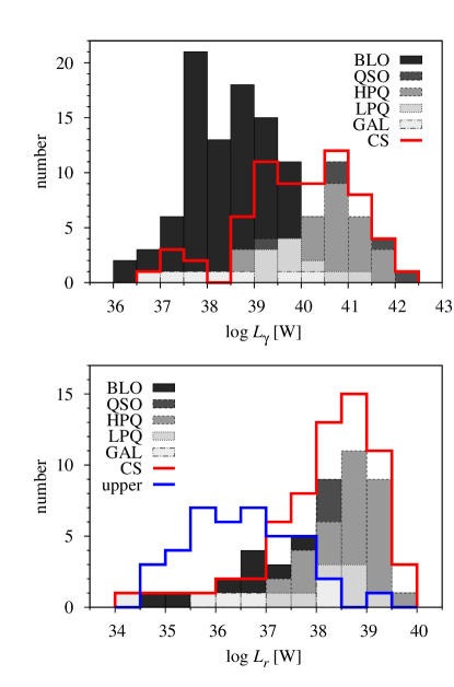
Figure 1: Distribution of the gamma-ray (top panel) and 37 GHz radio (bottom panel) luminosities in the different subsamples. 3C 274 at log $L_{\gamma}=34.8\mathrm{W}$ has been omitted from the top panel. CS in the legend stands for the complete northern sample.

Figure 1 shows the distribution of the Fermi/LAT $\gamma$-ray and 37 GHz luminosities. The subsamples are plotted with different shades to illustrate their differences. The luminosity distributions of the complete northern sample are also plotted separately with a red line (abbreviated as CS in the legend). It is clear that BLOs have lower gamma-ray luminosities than quasars. The few radio galaxies in the sample are quite evenly distributed, although 3C 274 (M 87) at log $L_{\gamma}=34.8$ W was omitted from the figure for clarity. Our complete northern sample is emphasized in the high-luminosity end. According to the Kruskal-Wallis test (performed with the Unistat statistical package v5.6.01), BLOs and galaxies are indeed drawn from a different gamma-ray luminosity distribution than all quasar subsamples.

The radio luminosity histogram shows very similar characteristics. Here the number of BLOs is much lower because of their typically faint and often undetected radio fluxes at 37 GHz. That is why we chose to plot also the distribution of the upper limit radio luminosities, calculated for sources with $S/N\leq 4$ non-detections during the 1FGL period (blue line in the figure). Most of these (31/40) are BLOs. When these upper limit luminosities are taken into consideration, we see that the distribution of the radio luminosities is very similar to that of the gamma-ray luminosities. No clear differences between the 37 GHz luminosity distributions of the subsamples are found with the Kruskal-Wallis test. However, including the upper limit data points in the analysis changes the result. We performed two sample tests for censored data with the ASURV Rev 1.3 software (Lavalley et al. 1992), which implements the methods for censored data presented in Isobe et al. (1986). According to logrank and Gehan’s generalized Wilcoxon tests, the final result is the same as with gamma luminosities, and BLOs differ from all quasars groups at the 5% level and share a similar parent distribution with galaxies.

In Fig. 2 we present the flux (top panel) and luminosity (bottom panel) correlations between the gamma and radio bands for the Metsähovi sample. Many of the sources only have upper limit radio fluxes and luminosities. The outlier data point in the luminosity correlation is 3C 274 (M 87), having clearly lower luminosities in both bands but still fitting in the general trend. Significant correlation between the flux densities is found using the Kendall’s tau test performed with the ASURV package. The flux correlation for the whole sample is strong with $\tau=0.195$ and $P<0.001$, where $\tau=0$ would indicate no correlation, and $P$ gives the probability of no correlation. Table 2 lists the correlation coefficients for subsamples. Radio galaxies were omitted from the subsamples due to very small sample size. The flux correlation is significant for all subsamples except for BLOs and LPQs, and very strong for the northern sample. Although not listed in Table 2, the correlation for the whole sample is also significant ($\tau=0.230$ and $P<0.001$) when only detections are included and the upper limit datapoints discarded.

It is evident in Fig. 2 that the errors in the gamma-ray flux densities increase towards the low-flux end. However, the errors in the 37 GHz flux densities are minimal, if at all visible. The net effect of errors for the shape of the correlation is small.

The appearance of the luminosity correlation is strikingly coherent. It is possible that it is in some measure created by the common dependence on redshift of the gamma and radio luminosities rather than their intrinsic correlation. Redshift bias and instrument flux limits are the two factors most likely to create spurious correlations (Elvis et al. 1978; Feigelson & Berg 1983; Muecke et al. 1997; Bloom 2008). In this study we have tried to alleviate their effect by including the upper limits in radio fluxes and luminosities and by using correlation tests taking the redshift bias into account. We calculated the significance of the luminosity correlation using the partial correlation method for censored data presented in Akritas & Siebert (1996). Even without the effect of redshift, the correlation is significant for the whole sample, complete northern sample, and all subsamples except for LPQs, which had a small sample size of 11 objects. The values of partial Kendall’s $\tau$ and probabilites are listed in Table 2.

Figure 2: The flux and luminosity correlations between 37 GHz and the Fermi band. Solid circles represent the complete northern sample, and 37 GHz upper limits are indicated by arrows.

Table 2: Partial Kendall’s $\tau$ -coefficients and probabilities for no correlation between 37 GHz and gamma-ray fluxes and luminosities.

	Flux correlation			Luminosity correlation
Class	Number	$\tau$	$P$	Number	$\tau$	$P$
All	141	0.195	$<0.001$	140	0.288	$<0.05$
BLO	57	0.152	0.095	56	0.188	$<0.05$
HPQ	34	0.414	$<0.001$	34	0.426	$<0.05$
LPQ	11	0.168	0.473	11	0.027	$>0.05$
QSO	32	0.302	0.015	32	0.295	$<0.05$
CS	67	0.310	$<0.001$	67	0.433	$<0.05$

It is noteworthy that the strength of both the flux and luminosity correlations is greatest for HPQs, then for QSOs and lowest for LPQs and BLOs. This effect was also noticed in León-Tavares et al. (2011) using monthly-averaged flux densities in the same bands. We acknowledge the possibility that the correlation strengths and significances may be influenced by chance, especially when the sample size is small. To test the effect, we ran a set of Monte Carlo analyses for the correlations, randomly picking the same number of sources as in each of the subgroups from the whole sample. After a thousand iterations we determined the distributions of $\tau$ and $P$ for these random samples of $N$ sources. The simulation revealed that for LPQs the probability of not finding significant correlation in either flux or luminosity is high, irrespective of their true behaviour. Thus we cannot make any definite statements about their correlation one way or the other. However, the significance of both flux and luminosity correlation for HPQs is very high. The probability of finding such a correlation by chance is very low, meaning that the observed correlation in flux and luminosity is real. In flux density, the probability of finding a better correlation by chance is only 1%. The situation for QSOs and BLOs is more complicated. In the case of flux density, the simulation results imply that we cannot say anything definite about them. For QSOs, the probability of finding a better correlation by chance is 21%, which means that the correlation found in our study can also be spurious. Considering the luminosity correlation, it must be remembered that in the simulations the underlying distribution from which the random samples are picked is strongly correlated (the whole sample, $\tau=0.288$ and $P<0.05$). Testing correlations with intermediate strength, like those of QSOs and BLOs, is meaningless because when picking randomly a large fraction of the sources from a strongly correlated sample, the resulting sample is also very likely correlated to some degree.

As León-Tavares et al. (2011) suspect, the difference in correlation strengths, if real, can be a result of the larger viewing angles of BLOs compared to QSOs and HPQs (Hovatta et al. 2009). Having a tighter flux and luminosity correlation for sources with extremely small viewing angles would agree well with the idea of gamma-rays originating in the jet. After all, when the jet is pointed towards us, the jet emission is all we see. We investigated this further by plotting the gamma-ray luminosity against the viewing angles from Hovatta et al. (2009). The result is shown in Fig. 3. We calculated the correlation with Spearman’s rank correlation test with the Unistat v5.6.01 package. The correlation is significant for the whole sample ($\rho=-0.594$ and $P<0.001$). Only two of the data points do not belong in the complete northern sample, so the correlation is strong for the complete sample as well. For the subsamples we find a significant correlation for both BLOs ($\rho=-0.762$ and $P=0.002$) and HPQs ($\rho=-0.419$ and $P=0.023$). For LPQs the correlation is insignificant, possibly due to small sample size of 7 sources.

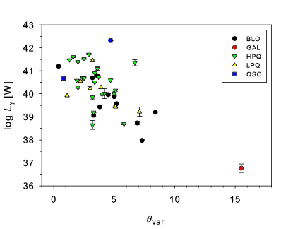
Figure 3: Luminosity in the Fermi band plotted against the viewing angle. For clarity, sources 3C 84 (GAL, log $L_{\gamma}=37.1$ W, $\theta_{var}=39.1$) and 3C 371.0 (BLO, log $L_{\gamma}=37.3$ W, $\theta_{var}=57.3$) have been omitted from the figure.

Figure 4 shows the dependence between the gamma-ray luminosity, $L_{\gamma}$, and the peak frequency of the synchrotron component, log $\nu_{p}$. The peak frequencies were preferably taken from Nieppola et al. (2008) and then from Nieppola et al. (2006). They are not from the same observational period as the Fermi data. However, because the log $\nu_{p}$ -values were calculated from averaged data, major shifts in log $\nu_{p}$ for a significant number of sources are unlikely. For 16 additional sources we took the peak frequency from Abdo et al. (2010a), who use data from the 1FGL period. The Spearman correlation coefficients for the log $L_{\gamma}$ – log $\nu_{p}$ correlation are $\rho=-0.706$ and $P<0.001$ for the whole sample and $\rho=-0.419$ and $P<0.001$ for the complete northern sample. Of the subsamples, the correlation is significant for BLOs and QSOs. When $\nu_{p}>14.5$, the sample consists of only BLOs, whose peak frequency range extends further into the high-energy region. As stated in Nieppola et al. (2006), the values of $\nu_{p}$ may be exaggerated toward the high-$\nu_{p}$ end. However, this does not change the main shape of the correlation in Fig. 4. The correlation would in fact only be stronger if the high-$\nu_{p}$ tail moved to lower frequencies.

Figure 4: The correlation between the gamma-ray luminosity, $L_{\gamma}$, and the peak frequency of the synchrotron component, $\nu_{p}$. Solid circles represent the complete northern sample.

4.2 Gamma dominance

In this paper we define gamma dominance as the ratio between the Fermi/LAT $\gamma$-ray and 37 GHz radio fluxes, $S_{\gamma}/S_{r}$. We emphasize that what we call gamma dominance is different from Compton dominance, which equals the ratio of the peak luminosities of the IC and synchrotron components of the SED. Figure 5 shows the distribution of the gamma dominance in our sample. Again, we drew the subsamples separately, and additionally plotted the distribution of the complete sample (red line). The gamma dominances of these samples were calculated using only the 37 GHz detections. For completeness, we have also plotted in the figure the distribution of the gamma dominances for the rest of the sample, which were calculated from upper limit average 37 GHz fluxes (resulting in lower limit gamma dominances, blue line in the figure). This lower limit sample contains BLOs for the most part (31/40), as well as five QSOs, two LPQs, and two GALs. Due to their low radio fluxes, the lower limit sources are located in the high end of the gamma dominance distribution. In contrast to the luminosity distributions (Fig. 1), all subsamples seem to have very similar distributions of gamma dominance. According to the Kruskal-Wallis test, QSOs are, however, signicantly different from others. The mean gamma dominance of QSOs is log $S_{\gamma}/S_{r}=2.3$ compared to log $S_{\gamma}/S_{r}=1.4-1.9$ of other subsamples.

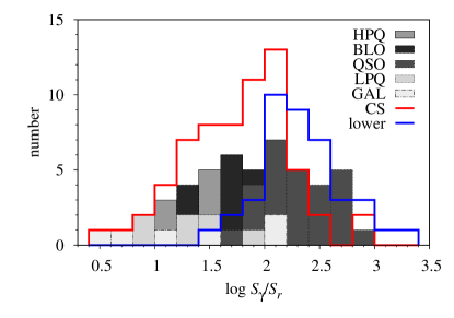
Figure 5: The distribution of the gamma dominance log $S_{\gamma}/S_{r}$. Different AGN subsamples are depicted with different shades, and the coloured lines mark the complete sample and the sources with only lower limit estimate of the gamma dominance.

In Fig. 6 we have plotted the gamma dominance against the synchrotron peak frequency $\nu_{p}$. Similarly to Fig. 4, objects beyond $\nu_{p}=14.5$ are exclusively radio-faint BLOs. In the whole sample there is a correlation ($\rho=0.537$ and $P<0.001$), but it disappears when only the complete sample is considered ($\rho=0.171$ and $P=0.173$). The positive correlation is also significant for BLOs, and just barely for the QSOs.

Figure 6: The gamma dominance plotted against the synchrotron peak frequency. Solid circles represent the complete northern sample.

In an effort to get hints of the main driver behind the gamma-ray emission, we incorporated several possible factors in the same plot. Fig. 7 includes gamma dominances, the apparent velocity of the jet, the brightness temperature $T_{b}$, the viewing angle $\theta$, and the Lorentz factor of the jet. The figure in its original form was published in Hovatta et al. (2009). We have added the gamma dominance to trace its dependence on the jet parameters. For completeness, we also included sources not detected by Fermi.

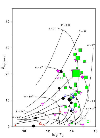
Figure 7: The AGN sample of Hovatta et al. (2009) plotted as a function of apparent speed $\beta$, the brightness temperature $T_{b}$, the viewing angle $\theta$, and the Lorentz factor $\Gamma$. Open symbols are not detected by Fermi, filled symbols are detected, and the size of the symbol is proportional to the gamma dominance. Red triangles are galaxies, black circles BLOs, pink inverted triangles LPQs, green squares HPQs, and purple diamonds QSOs.

The stronger gamma-ray dominance of QSOs is not evident in the figure because the sample size of QSOs is significantly reduced by the requirement of the jet parameters. This selection effect influences the whole sample in the figure, which must be remembered when interpreting it. The jet parameters are calculated from flares in the 22 or 37 GHz flux curves (Hovatta et al. 2009), so all results only apply for radio-bright, flaring sources and not categorically to all gamma-ray emitters. However, closer inspection reveals two things. The gamma-detected and -dominated sources have generally very small viewing angles and high brightness temperatures. Also at least the probability of gamma-ray detection grows with increasing $\Gamma$. However, there is no single property singling out the gamma-dominated sources. We conclude, like others before us (e.g., Lister et al. 2009; Savolainen et al. 2010), that jet parameters play an important role in the gamma-ray emission of radio-bright AGN.

4.3 Variability

It has been noted previously that AGN detected by Fermi are often flaring in radio or at least in an active state (i.e., variable) (Kovalev et al. 2009; Tornikoski et al. 2010). Recently, Richards et al. (2011) have carried out a detailed statistical study of differences in the variability amplitudes of gamma-ray detected and non-detected sources. They found that gamma-ray detected sources almost have a factor of two higher variability amplitude than sources not detected by Fermi .

However, among the gamma-ray detected sources, the brightest ones do not seem to be any more variable at 37 GHz during the 1FGL period than fainter ones. This is seen in Fig. 8 and confirmed by Spearman rank correlation test. The variability index at 37 GHz we used in Fig. 8 is

$$S_{var}=\frac{S_{max}-S_{min}}{S_{max}+S_{min}},$$ (3)

where $S_{max}$ and $S_{min}$ are the maximum and minimum flux densities, respectively, during the variability period. However, the 1-year 1FGL period is a very short time when trying to illustrate AGN variability accurately. The variability index tends to get higher with increasing observing time, which is why we replotted the figure using the entire Metsähovi database. The distribution of the datapoints remained very similar, but the population is moved toward higher $S_{var}$. Any significant correlation did not appear.

Figure 8: The dependence between the variability at 37 GHz during the 1FGL period and the gamma-ray luminosity. Solid circles represent the complete northern sample.

5 Discussion

The undisputed correlation between the Fermi/LAT $\gamma$-ray and 37 GHz radio luminosities presented in this paper (Fig. 2) is a strong indication of the common origin of high radio frequency and gamma-ray radiation in AGN. The flux correlation, mostly at lower radio frequencies, has also been presented by other authors. Giroletti et al. (2010) find a dependence between the Fermi/LAT and 8.4 Jy flux densities from the CRATES catalogue (Healey et al. 2007). Mahony et al. (2010) used the 20 GHz data (closer to ours in frequency) taken with the Australia Telescope Compact Array and, again, find a significant correlation. This 20 GHz correlation was studied in depth by Ghirlanda et al. (2011), who use a numerical simulation to conclude that the flux correlation is actually real and not an effect of instrument flux limits. They also observe a tight luminosity correlation. In their data, the flux correlation for BLOs is significant, whereas in our 37 GHz data the correlation is rejected at the 5% level. This is most likely due to the high number (almost half) of upper limits in our BLO radio fluxes, which may weaken the correlation.

A significant luminosity correlation was also noted by Bloom (2008) using CGRO/EGRET data and applying Monte Carlo simulations. EGRET data were used earlier by Muecke et al. (1997). They thoroughly studied the luminosity correlations through simulations and in practice between EGRET and Effelsberg 100m radio telescope data. In contrast to the later studies listed above, they found no correlation in any of the frequency bands (2.7, 4.8, 8, and 10 GHz). They considered simultaneous, maximum, and mean fluxes separately. One possible explanation for the correlation not appearing in their data is the use of relatively low radio frequencies. Below 15 GHz, the features in the flux curves are less distinct because the individual shock components are superposed. The emission typically is significantly delayed compared to the higher frequency bands, even 181 days at 4.8 GHz with respect to the flare peak at a higher radio frequency (Hovatta et al. 2008). Naturally, the correlation between low radio frequency flux and gamma-ray flux would be very difficult to detect, even if such a connection exists. The same effect is evident in Richards et al. (2010), who compare Fermi data with simultaneous F-GAMMA project data. The flux correlation is tested with IRAM, Effelsberg, and OVRO data between 2.6 and 142 GHz. For frequencies above 10.5 GHz, the correlation is significant, but it cannot be confirmed for the lower frequencies.

In Nieppola et al. (2008) we observed that the inverse correlation between the synchrotron peak frequency and luminosity, a part of the blazar sequence scenario (Fossati et al. 1997; Ghisellini et al. 1998; Ghisellini & Tavecchio 2008) and often observed for radio-bright blazars, can naturally be explained by the stronger Doppler boosting of low-$\nu_{p}$ sources. Once corrected for boosting, blazars show no correlation between the two quantities, and there is even an indication that high-$\nu_{p}$ blazars may have brighter synchrotron peaks in the rest frame. If we consider the correlation between radio and gamma-ray luminosities (Fig. 2) and between gamma-ray luminosity and the viewing angle (Fig. 3), it seems only natural that similar boosting also affects the gamma-ray emission. Stronger boosting of gamma-ray bright sources was also suspected by Lähteenmäki & Valtaoja (2003) and Fermi -detected AGN have been found more boosted than the non-detected by several authors (e.g., Kovalev et al. 2009; Savolainen et al. 2010). Therefore we consider it very possible that the correlation between $\nu_{p}$ and $L_{\gamma}$ would disappear if intrinsic values could be used. It is also well known that the limiting flux of the LAT telescope is a function of the photon spectral index (Abdo et al. 2010c). This means that it is more likely to detect faint sources with hard photon indices than with soft ones (see Fig. 9 of Abdo et al. 2010c). This probably explains a part of the different distributions of the subgroups in gamma luminosity, but does not account for the fact that sources of high Fermi luminosity are mostly quasars.

Strong Doppler boosting in the Fermi -band would also offer an explanation for the stronger gamma dominance of high-$\nu_{p}$ sources (Fig. 6). If the intrinsic synchrotron and Compton luminosities across the $\nu_{p}$-range were comparable, the Fermi luminosities for high-$\nu_{p}$ sources would be higher, on average. This is because the SED of low-$\nu_{p}$ sources is already falling in the Fermi band, while that of the high-$\nu_{p}$ sources is just peaking. This would result in stronger gamma-dominance in high-$\nu_{p}$ sources, as indicated. After all, being a ratio of fluxes, the gamma dominance is much less dependent on Doppler boosting, although spectral indices and the difference in Doppler factors in radio and gamma regions play a role.

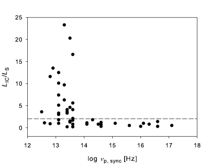
Figure 9: The Compton dominance plotted against the synchrotron peak frequency, both data sets from Abdo et al. (2010a). Sources above the dashed line at $L_{IC}/L_{s}=2$ are Compton dominated according to the classification of Abdo et al. (2010a).

The role of Doppler boosting in the gamma region has not been studied with observational data owing to the difficulty of measuring the amount of boosting at high energies. The Compton dominance, $L_{IC}/L_{s}$, measured from robust SEDs for an extensive sample would also give a measure of the differences between the peak intensities. The best data set available for such a study is that of Abdo et al. (2010a). There the Compton dominance is calculated for 48 sources. When plotted against log  $\nu_{p}$, it is evident that the highest Compton dominances occur at low $\nu_{p}$ (Fig. 9). The low Compton dominances, in turn, are evenly spread in the $\nu_{p}$-range. Abdo et al. (2010a) define objects with $L_{IC}/L_{s}>2$ as Compton dominated. While all Compton dominated sources are low synchrotron-peaked blazars (LSP), they also form the biggest group among the non-Compton dominated sources. It seems that the correlation between $\nu_{p}$ and Compton dominance is far from simple. Tramacere et al. (2010) suggest that quasars with strong Compton domination have intrinsically different emission mechanism (EC) than sources (including LSP) with low Compton domination (SSC). Also Lähteenmäki & Valtaoja (2003) suspect that quasars and BLOs may have different mechanisms for gamma-ray emission. They, however, reach the conclusion that BLOs are weaker gamma emitters, and most likely at least a part of their emission is produced via the EC process, contrary to the scheme of Tramacere et al. (2010). We hope the new data releases from Fermi will help in resolving these issues.

6 Summary

We have connected data from Fermi/LAT 1FGL catalogue with the 37 GHz observations from Aalto University Metsähovi Radio Observatory for 249 northern AGN through flux and luminosity correlations. We also calculated the gamma dominances and compared them, along with the gamma-ray luminosities, with the synchrotron peak frequency. From our results we draw the following summary:

1. The 37 GHz luminosities are significantly lower for BLOs than for quasar subsamples. A similar result for the Fermi luminosities has been found in earlier studies and corroborated by our data.

2. We find significant correlation between the Fermi/LAT and 37 GHz flux densities for our whole sample ($\tau=0.195$ and $P<0.001$) and the complete northern sample ($\tau=0.310$ and $P<0.001$), as well as HPQ and QSOs. For BLOs and LPQs the correlation is not significant.

3. We find a significant correlation for Fermi/LAT and 37 GHz luminosities for the whole sample ($\tau=0.288$ and $P<0.05$) and all subsamples except for LPQs.

4. There is a strong negative correlation between the viewing angle and the average Fermi luminosity, for the whole sample, as well as for BLOs and HPQs alone.

5. The gamma-ray luminosities of high-synchrotron peaked blazars are lower than those of low-synchrotron peaked blazars, but high-peaked blazars seem to be more gamma-ray dominated when using the Fermi/LAT and 37 GHz bands. This could be explained with the significantly stronger Doppler boosting of low-synchrotron peaked blazars in the gamma region.

6. The long-term 37 GHz variability does not depend on the gamma-ray luminosity; i.e., high Fermi luminosity objects are not more variable at 37 GHz.

7. As found in previous studies, we also conclude that BLOs are different gamma-ray emitters than quasars. This may be the result of stronger Doppler boosting for quasars or of inherently different emission mechanisms.

8. Our results support the view that gamma-rays are produced co-spatially with the 37 GHz radiation, i.e., in the jet, mainly through the SSC process. Co-spatial origin of radio and gamma-ray emission would also serve as a natural explanation of the possibly similar relativistic boosting properties in the two bands.

Table 3: The sample sources used in this study and their classifications.

Name	1FGL name	Class	Complete sample	R.A.(J2000)	Dec(J2000)	$z$	$S_{r}$	log $S_{\gamma}$
							$[\textrm{Jy}]$	$[\textrm{erg cm}^{-2}\textrm{s}^{-1}]$
CGRaBS J0017–0512	J0017.4–0510	QSO	…	4.37	–5.18	…	0.42	…
RX J0018.4+2947	J0018.6+2945	BLO	…	4.65	29.76	0.10	…	–10.80
PKS 0017+200	J0019.3+2017	BLO	…	4.83	20.29	…	…	…
PKS 0019+058	J0022.5+0607	BLO	…	5.63	6.13	…	0.28	…
RX J0035.2+1515	J0035.1+1516	BLO	…	8.79	15.27	1.09	…	–10.86
1ES 0033+595	J0035.9+5951	BLO	…	8.99	59.85	0.09	$<0.28$	–10.48
0039+230	J0041.9+2318	…	…	10.48	23.31	1.43	…	–10.75
RX J0045.3+2127	J0045.3+2127	BLO	…	11.34	21.46	…	…	…
PKS 0047+023	J0050.2+0235	BLO	…	12.55	2.59	…	…	…
0048–097	J0050.6–0928	BLO	C	12.66	–9.48	0.30	1.36	–10.27
PKS 0048–071	J0051.1–0649	QSO	…	12.78	–6.82	1.97	1.18	–10.53
J0100+0745	J0100.2+0747	…	…	15.05	7.80	…	…	…
0059+581	J0102.8+5827	HPQ	C	15.71	58.47	0.64	3.28	–10.27
0106+013	J0108.6+0135	HPQ	C	17.17	1.59	2.10	2.12	–9.82
RGB J0109+182	J0109.0+1816	BLO	…	17.26	18.28	0.15	…	–11.16
S2 0109+22	J0112.0+2247	BLO	…	18.02	22.79	0.27	$<0.9$	–10.34
4C 31.03	J0112.9+3207	QSO	…	18.23	32.12	0.60	1.06	–10.06
RX J0115.7+2519	J0115.5+2519	BLO	…	18.89	25.33	0.37	…	–10.85
B3 0133+388	J0136.5+3905	BLO	…	24.13	39.09	…	$<0.56$	…
0133+476	J0137.0+4751	HPQ	C	24.25	47.85	0.86	3.50	–9.89
PKS 0139–09	J0141.7–0929	BLO	…	25.43	–9.49	0.73	$<0.36$	–10.85
J0144+2705	J0144.6+2703	…	…	26.17	27.06	…	…	…
RX J0159.5+1047	J0159.5+1047	BLO	…	29.89	10.80	…	…	…
RX J0202.4+0849	J0202.1+0849	BLO	…	30.53	8.83	…	…	…
S5 0159+72	J0203.5+7234	BLO	…	30.89	72.57	…	$<0.48$	…
0202+149	J0204.5+1516	HPQ	C	31.13	15.28	0.41	0.68	–11.13
MS 0205.7+3509	J0208.6+3522	BLO	…	32.17	35.38	0.32	…	–10.97
J0211+1051	J0211.2+1049	QSO	…	32.81	10.83	…	0.71	…
Zel 0214+083	J0217.2+0834	BLO	…	34.32	8.58	1.40	…	–10.93
0212+735	J0217.8+7353	HPQ	C	34.45	73.88	2.37	2.45	–10.31
0215+015	J0217.9+0144	HPQ	…	34.48	1.75	1.72	1.37	–10.18
0218+357	J0221.0+3555	BLO	…	35.27	35.93	0.94	0.91	–10.04
3C 66A	J0222.6+4302	BLO	…	35.67	43.04	0.44	$<0.8$	–9.57
0234+285	J0237.9+2848	HPQ	C	39.49	28.80	1.21	2.71	–10.04
0235+164	J0238.6+1637	BLO	C	39.67	16.62	0.94	3.84	–9.47
S5 0238+71	J0243.5+7116	BLO	…	40.89	71.28	…	$<0.4$	…
RX J0250.6+1712	J0250.4+1715	BLO	…	42.61	17.26	1.10	$<0.16$	–10.96
4C 47.08	J0303.1+4711	BLO	…	45.79	47.19	0.48	1.11	–10.82
RX J0316.1+0904	J0316.1+0904	BLO	…	49.05	9.08	…	…	…
MS 0317.0+1834	J0319.7+1847	BLO	…	49.93	18.80	0.19	…	–10.79
3C 84	J0319.7+4130	GAL	C	49.94	41.51	0.02	14.28	–9.76
RGB J0321+2336	J0322.1+2336	BLO	…	50.54	23.61	…	…	…
2E 0323+0214	J0326.2+0222	BLO	…	51.57	2.38	0.15	…	–10.89
CTA 026	J0339.2–0143	HPQ	C	54.80	–1.72	0.85	1.89	–10.70
2E 0414+0057	J0416.8+0107	BLO	…	64.21	1.12	0.29	…	–10.81
0415+379	J0419.0+3811	GAL	C	64.76	38.19	0.05	5.19	–10.99
PKS 0420+022	J0422.1+0211	BLO	…	65.53	2.20	2.28	0.67	–10.73
0420–014	J0423.2–0118	HPQ	C	65.80	–1.31	0.92	4.96	–10.05
PKS 0422+0036	J0424.8+0036	BLO	…	66.21	0.61	0.31	0.75	–10.85
2EG J0432+2910	J0433.5+2905	BLO	…	68.39	29.09	…	$<0.44$	…
NRAO 190	J0442.7–0019	QSO	…	70.69	–0.32	0.84	0.89	–9.98
PKS 0446+112	J0448.6+1118	GAL	C	72.17	11.31	1.21	0.73	–10.49
PKS 0458–020	J0501.0–0200	HPQ	C	75.27	–2.00	2.29	1.01	–10.53
RX J0505.5+0416	J0505.2+0420	BLO	…	76.31	4.34	0.03	…	–10.81
1ES 0502+675	J0507.9+6738	BLO	…	76.99	67.64	0.31	$<0.44$	–10.48
0506+101	J0509.2+1015	…	…	77.31	10.26	…	0.64	…
MG 0509+0541	J0509.3+0540	BLO	…	77.34	5.67	…	…	…
0507+179	J0510.0+1800	HPQ	C	77.50	18.02	0.42	1.27	–11.04
0528+134	J0531.0+1331	HPQ	C	82.75	13.52	2.07	2.32	–9.91
0539–057	J0540.9–0547	LPQ	…	85.23	–5.79	0.84	$<0.71$	–10.79
PKS 0605–085	J0608.2–0837	HPQ	C	92.05	–8.62	0.87	1.98	–10.59
0621+446	J0625.4+4440	BLO	…	96.36	44.67	…	$<0.36$	…
1ES 0647+250	J0650.7+2503	BLO	…	102.68	25.06	0.20	…	–10.74
B3 0650+453	J0654.3+4514	QSO	…	103.58	45.25	0.93	…	–10.09
J0654+5042	J0654.4+5042	…	…	103.62	50.71	…	$<0.39$	…
EXO 0706.1+591	J0710.6+5911	BLO	…	107.66	59.19	0.13	…	–10.87
J0712+5033	J0712.7+5033	BLO	…	108.18	50.56	…	$<0.56$	…
J0713+1935	J0714.0+1935	…	…	108.51	19.59	…	0.70	…
0716+332	J0719.3+3306	QSO	…	109.85	33.11	0.78	0.39	–10.24
0718+042	J0721.4+0401	…	…	110.35	4.03	…	0.73	…
0716+714	J0721.9+7120	BLO	C	110.48	71.34	0.30	2.38	–9.89
RX J0723.2+5841	J0722.3+5837	BLO	…	110.59	58.63	…	…	…
PKS 0723–008	J0725.9–0053	GAL	C	111.50	–0.90	0.13	2.45	–10.90
FBQS J0730+3307	J0730.0+3305	BLO	…	112.52	33.09	0.11	…	–10.90
PKS 0735+17	J0738.2+1741	BLO	C	114.56	17.70	0.42	$<0.69$	–10.40
0736+017	J0739.1+0138	HPQ	C	114.79	1.64	0.19	1.56	–10.33
0738+5451	J0742.2+5443	QSO	…	115.56	54.73	0.72	0.62	–10.57
MS 0737.9+7441	J0745.2+7438	BLO	…	116.32	74.64	0.32	…	–11.02
J0746.3+2548	J0746.6+2548	QSO	…	116.66	25.80	2.98	$<0.37$	–10.35
0748+126	J0750.6+1235	LPQ	C	117.67	12.59	0.89	3.55	–10.62
S4 0749+54	J0752.8+5353	BLO	…	118.20	53.89	0.20	0.54	–10.97
0754+100	J0757.2+0956	BLO	C	119.31	9.94	0.27	1.28	–10.61
RX J0805.4+7534	J0804.7+7534	BLO	…	121.19	75.57	0.12	…	–10.86
0805–077	J0808.2–0750	QSO	C	122.05	–7.84	1.84	1.48	–9.98
1ES 0806+524	J0809.5+5219	BLO	…	122.39	52.32	0.14	$<0.34$	–10.54
PKS 0808+019	J0811.2+0148	BLO	…	122.81	1.82	0.93	0.79	–10.80
RX J0816.3+5739	J0816.7+5739	BLO	…	124.19	57.66	…	…	…
0814+425	J0818.2+4222	BLO	…	124.55	42.38	0.25	1.43	–10.06
0820+560	J0825.0+5555	HPQ	…	126.27	55.93	1.42	0.74	–10.33
0823+033	J0825.9+0309	HPQ	C	126.49	3.15	0.51	1.22	–10.97
OJ 248	J0830.5+2407	LPQ	C	127.63	24.12	0.94	$<1.32$	–10.39
0829+046	J0831.6+0429	BLO	…	127.91	4.49	0.18	$<0.62$	–10.54
0836+710	J0842.2+7054	LPQ	C	130.57	70.90	2.17	2.10	–10.13
RX J0847.2+1133	J0847.2+1134	BLO	…	131.82	11.57	0.20	$<0.24$	–10.94
J0850–1213	J0850.0–1213	QSO	…	132.52	–12.22	0.57	0.59	–10.55
OJ 287	J0854.8+2006	BLO	C	133.71	20.11	0.31	5.94	–10.42
Ton 1015	J0910.7+3332	BLO	…	137.68	33.54	0.35	…	–10.97
B2 0912+29	J0915.7+2931	BLO	…	138.94	29.53	…	…	…
0917+449	J0920.9+4441	QSO	C	140.24	44.69	2.18	2.44	–9.69
J0948+0022	J0949.0+0021	GAL	…	147.25	0.36	0.58	$<0.6$	–10.18
0953+254	J0956.9+2513	LPQ	C	149.24	25.22	0.71	0.75	–10.97
S4 0954+556	J0957.7+5523	HPQ	…	149.43	55.39	0.90	0.77	–9.97
S4 0954+65	J1000.1+6539	BLO	C	150.03	65.65	0.37	$<1.09$	–10.98
EXO 1004.0+350	J1007.0+3454	BLO	…	151.77	34.90	0.61	…	–10.97
NRAO 350	J1012.2+0634	BLO	…	153.06	6.57	0.73	…	–10.82
GB 1011+496	J1015.1+4927	BLO	…	153.79	49.45	0.20	$<0.4$	–10.07
1013+054	J1016.1+0514	QSO	…	154.03	5.24	1.71	0.44	–10.03
RX J1022.7–0112	J1022.8–0115	BLO	…	155.72	–1.25	…	…	…
1ES 1028+511	J1031.0+5051	BLO	…	157.76	50.86	0.36	$<0.36$	–10.96
B3 1029+378	J1032.7+3737	BLO	…	158.18	37.63	…	…	…
J 1033+6051	J1033.8+6048	QSO	…	158.47	60.80	…	…	…
RX J1037.7+5711	J1037.7+5711	BLO	…	159.44	57.20	…	…	…
TXS 1040+244	J1043.1+2404	BLO	C	160.79	24.08	0.56	1.24	–10.96
MS 1050.7+4946	J1053.6+4927	BLO	…	163.42	49.45	0.14	$<0.36$	–10.79
J1054+2210	J1054.5+2212	…	…	163.63	22.21	…	$<0.16$	…
1055+018	J1058.4+0134	HPQ	C	164.62	1.58	0.89	4.48	–10.01
1055+567	J1058.6+5628	QSO	…	164.67	56.48	0.14	$<0.28$	–10.18
Mrk 421	J1104.4+3812	BLO	…	166.12	38.21	0.03	$<0.42$	–9.51
RX J1110.6+7133	J1109.9+7134	BLO	…	167.50	71.58	…	…	…
RX J1117.0+2014	J1117.1+2013	BLO	…	169.30	20.22	0.10	…	–10.64
EXO 1118.0+422	J1121.0+4209	BLO	…	170.25	42.16	0.12	…	–10.93
1118–056	J1121.5–0554	QSO	…	170.38	–5.91	1.30	$<0.42$	–10.33
RX J1136.5+6737	J1136.2+6739	BLO	…	174.06	67.66	0.14	…	–10.92
Mrk 180	J1136.6+7009	BLO	…	174.16	70.16	0.05	$<0.24$	–10.78
RX J1136.8+2551	J1136.9+2551	BLO	…	174.24	25.86	0.20	…	–10.81
B2 1147+24	J1150.2+2419	BLO	…	177.57	24.32	0.20	0.77	–10.89
RX J1151.4+5859	J1151.6+5857	BLO	…	177.91	58.96	…	…	…
4C 29.45	J1159.4+2914	HPQ	C	179.85	29.24	0.73	2.64	–10.13
B3 1206+416	J1209.4+4119	BLO	…	182.37	41.32	…	$<0.36$	…
B2 1215+30	J1217.7+3007	BLO	…	184.45	30.12	0.24	$<0.47$	–10.21
GB2 1217+348	J1220.2+3432	BLO	…	185.06	34.53	0.13	…	–11.14
PG 1218+304	J1221.3+3008	BLO	…	185.34	30.14	0.18	$<0.27$	–10.44
ON 231	J1221.5+2814	BLO	…	185.39	28.25	0.10	$<0.42$	–10.17
1219+044	J1222.5+0415	QSO	C	185.64	4.27	0.97	1.00	–10.60
PKS 1222+216	J1224.7+2121	LPQ	C	186.20	21.36	0.44	0.87	–10.41
S5 1221+80	J1224.8+8044	BLO	…	186.22	80.74	…	…	…
3C 273	J1229.1+0203	HPQ	C	187.28	2.05	0.16	23.35	–9.64
3C 274	J1230.8+1223	GAL	C	187.72	12.39	0.00	14.03	–10.76
B2 1229+29	J1231.6+2850	BLO	…	187.90	28.83	1.00	…	–10.60
1237+0459	J1239.5+0443	QSO	…	189.89	4.72	1.76	0.33	–10.22
Ton 116	J1243.1+3627	BLO	…	190.79	36.46	1.07	…	–10.63
PG 1246+586	J1248.2+5820	BLO	…	192.06	58.34	0.85	$<0.44$	–10.23
S4 1250+53	J1253.0+5301	BLO	…	193.26	53.02	…	$<0.4$	…
3C 279	J1256.2–0547	HPQ	C	194.05	–5.79	0.54	14.87	–9.36
MC2 1307+12.1	J1309.2+1156	BLO	…	197.31	11.94	…	…	…
1308+326	J1310.6+3222	BLO	C	197.65	32.37	1.00	2.57	–10.03
TXS 1312+240	J1314.7+2346	BLO	…	198.68	23.77	…	…	…
1324+224	J1326.6+2213	QSO	C	201.65	22.22	1.40	0.77	–10.43
PKS 1329–049	J1331.9–0506	QSO	…	202.99	–5.11	2.15	1.18	–9.83
J1333+5057	J1333.2+5056	…	…	203.30	50.95	…	0.24	…
1334–127	J1337.7–1255	LPQ	…	204.43	–12.93	0.54	5.93	–10.38
RX J1340.4+4410	J1340.6+4406	BLO	…	205.17	44.12	0.54	…	–11.10
B2 1338+40	J1341.3+3951	BLO	…	205.33	39.85	0.16	…	–10.97
PKS 1352–104	J1354.9–1041	QSO	…	208.73	–10.69	0.33	$<0.68$	–10.50
1357+769	J1358.1+7646	QSO	…	209.53	76.77	…	$<0.4$	…
PKS 1406–076	J1408.9–0751	QSO	…	212.23	–7.85	1.49	0.76	–10.44
2E 1415+2557	J1417.8+2541	BLO	…	214.46	25.68	0.24	…	–11.09
RX J1422.6+5801	J1422.2+5757	BLO	…	215.56	57.96	0.64	…	–10.97
RX J1426.1+3404	J1426.0+3403	BLO	…	216.52	34.06	…	…	…
PKS 1424+240	J1426.9+2347	BLO	…	216.75	23.80	0.16	$<0.46$	–9.90
H 1426+428	J1428.7+4239	BLO	…	217.18	42.66	0.13	$<0.29$	–10.75
RX J1436.9+5639	J1437.0+5640	BLO	…	219.26	56.67	0.15	…	–10.99
PG 1437+398	J1439.2+3930	BLO	…	219.81	39.50	0.35	…	–10.98
1ES 1440+122	J1442.8+1158	BLO	…	220.71	11.97	0.16	…	–10.87
RX J1448.0+3608	J1447.9+3608	BLO	…	221.99	36.15	…	…	…
SBS 1452+516	J1454.6+5125	BLO	…	223.66	51.42	1.08	…	–10.64
MS 1458.8+2249	J1501.1+2237	BLO	…	225.28	22.62	0.24	…	–10.63
PKS 1502+106	J1504.4+1029	QSO	C	226.10	10.49	1.84	2.90	–9.08
1502+036	J1505.0+0328	QSO	…	226.27	3.47	0.41	0.56	–10.57
SBS 1508+561	J1509.4+5602	BLO	…	227.35	56.04	1.68	…	–10.88
PKS 1508–055	J1511.1–0545	QSO	…	227.79	–5.76	1.19	0.94	–10.57
PKS 1510–089	J1512.8–0906	HPQ	C	228.21	–9.10	0.36	2.77	–9.15
PKS 1514+197	J1516.9+1928	BLO	…	229.25	19.48	0.65	1.63	–10.90
1H 1515+660	J1517.8+6530	BLO	…	229.46	65.51	0.70	…	–11.09
J1522+3144	J1522.1+3143	QSO	…	230.55	31.73	…	$<0.4$	…
RX J1532.0+3016	J1531.8+3018	BLO	…	232.96	30.31	0.06	…	–10.95
1541+8204	J1536.6+8200	…	…	234.15	82.01	…	…	…
RX J1542.9+6129	J1542.9+6129	BLO	…	235.74	61.49	…	…	…
1546+027	J1549.3+0235	HPQ	C	237.34	2.60	0.41	1.74	–10.46
1548+056	J1550.7+0527	HPQ	C	237.68	5.46	1.42	2.10	–11.01
PKS 1551+130	J1553.4+1255	QSO	…	238.36	12.93	1.29	0.59	–10.06
PG 1553+11	J1555.7+1111	BLO	…	238.94	11.19	0.36	$<0.29$	–9.77
MYC 1557+566	J1558.9+5627	BLO	…	239.74	56.46	0.30	…	–10.73
PKS 1604+159	J1607.1+1552	BLO	…	241.79	15.87	0.36	0.48	–10.63
1606+106	J1609.0+1031	LPQ	C	242.25	10.53	1.23	0.89	–10.41
DA 406	J1613.5+3411	HPQ	C	243.39	34.19	1.40	2.02	–11.09
4C 38.41	J1635.0+3808	HPQ	C	248.77	38.14	1.81	3.06	–9.86
3C 345	J1642.5+3947	HPQ	C	250.64	39.79	0.59	7.12	–10.02
Mrk 501	J1653.9+3945	BLO	C	253.49	39.75	0.03	1.01	–9.99
J1700+6830	J1700.1+6830	QSO	…	255.05	68.51	0.30	$<0.46$	–10.39
PKS 1717+177	J1719.2+1745	BLO	…	259.81	17.76	0.14	$<0.59$	–10.39
B 21722+40	J1724.0+4002	BLO	…	261.01	40.04	1.05	0.87	–10.46
H 1722+119	J1725.0+1151	BLO	…	261.27	11.86	0.02	…	–10.38
ZW I 187	J1727.9+5010	BLO	…	262.00	50.18	0.06	…	–10.93
PKS 1725+044	J1728.2+0431	GAL	…	262.07	4.52	0.29	$<1.08$	–10.55
1730–130	J1733.0–1308	LPQ	…	263.27	–13.14	0.90	3.65	–10.37
S4 1739+52	J1740.0+5209	HPQ	C	265.02	52.16	1.38	1.11	–9.96
RGB J1742+597	J1742.1+5947	BLO	…	265.54	59.80	0.40	…	–10.93
NPM1G +19.0510	J1744.2+1934	BLO	…	266.07	19.57	0.08	$<0.2$	–11.08
1741–038	J1744.6–0354	HPQ	C	266.15	–3.91	1.05	2.44	–10.76
S4 1749+70	J1748.5+7004	BLO	…	267.13	70.08	0.77	…	–10.70
B3 1747+433	J1749.0+4323	BLO	…	267.27	43.39	…	…	…
PKS 1749+096	J1751.5+0937	BLO	C	267.89	9.63	0.32	6.28	–10.10
RX J1756.2+5522	J1756.6+5524	BLO	…	269.15	55.40	…	…	…
S5 1803+784	J1800.4+7827	BLO	C	270.12	78.47	0.68	1.94	–10.36
3C 371.0	J1807.0+6945	BLO	C	271.75	69.76	0.05	1.21	–10.50
B2 1811+31	J1813.4+3141	BLO	…	273.36	31.69	0.12	…	–10.71
4C 56.27	J1824.0+5651	BLO	C	276.01	56.87	0.66	1.54	–10.41
1828+487	J1829.8+4845	LPQ	C	277.47	48.75	0.69	2.31	–11.12
RX J1829.4+5403	J1829.8+5404	BLO	…	277.47	54.08	…	…	…
RX J1838.7+4802	J1838.6+4756	BLO	…	279.66	47.95	…	…	…
J1849+6705	J1849.3+6705	GAL	C	282.32	67.09	0.66	3.50	–9.78
1851+488	J1852.5+4853	QSO	…	283.14	48.90	1.25	0.45	–10.60
RX J1903.1+5540	J1903.0+5539	BLO	…	285.77	55.65	…	…	…
RX J1931.1+0937	J1931.2+0939	BLO	…	292.81	9.65	…	…	…
1ES 1959+650	J2000.0+6508	BLO	…	300.02	65.13	0.05	$<0.5$	–10.10
S5 2007+77	J2006.0+7751	BLO	C	301.51	77.86	0.34	$<0.91$	–10.78
S5 2010+72	J2009.1+7228	BLO	…	302.29	72.47	…	0.44	…
PKS 2012–017	J2015.3–0129	BLO	…	303.83	–1.49	0.52	$<0.2$	–10.73
J2017+0603	J2017.3+0603	…	…	304.34	6.06	…	$<0.16$	…
PKS 2022–077	J2025.6–0735	QSO	…	306.42	–7.60	1.39	1.18	–9.68
PKS 2032+107	J2035.4+1100	BLO	…	308.86	11.00	0.60	0.62	–10.41
J2049+1003	J2049.7+1003	…	…	312.44	10.05	…	0.39	…
PKS 2047+039	J2050.1+0407	BLO	…	312.54	4.13	…	0.38	…
RBS 1752	J2131.7–0914	BLO	…	322.93	–9.24	0.45	…	–11.00
2131–021	J2134.0–0203	HPQ	C	323.51	–2.06	1.29	1.83	–11.08
2141+175	J2143.4+1742	QSO	…	325.87	17.72	0.21	0.75	–10.08
2144+092	J2147.2+0929	QSO	…	326.82	9.50	1.11	0.94	–9.96
2145+067	J2148.5+0654	LPQ	C	327.13	6.90	0.99	4.72	–10.81
PKS 2149+17	J2152.5+1734	BLO	…	328.14	17.58	…	0.43	…
2155+312	J2157.4+3129	QSO	…	329.37	31.50	1.49	0.74	–10.36
BL Lac	J2202.8+4216	BLO	C	330.72	42.28	0.07	2.91	–10.09
2201+171	J2203.5+1726	QSO	C	330.88	17.44	1.08	1.03	–10.16
PKS 2209+236	J2212.1+2358	QSO	…	333.03	23.97	1.12	0.71	–10.88
3C 446	J2225.8–0457	BLO	C	336.47	–4.96	1.40	6.89	–10.31
2227–088	J2229.7–0832	HPQ	C	337.44	–8.53	1.56	2.77	–9.83
2230+114	J2232.5+1144	HPQ	C	338.13	11.74	1.04	4.71	–10.04
2234+282	J2236.2+2828	HPQ	C	339.06	28.47	0.80	1.26	–10.21
RGB J2243+203	J2244.0+2021	BLO	…	341.01	20.36	…	…	…
B3 2247+381	J2250.1+3825	BLO	…	342.53	38.43	0.12	$<0.32$	–10.76
3C 454.3	J2253.9+1608	HPQ	C	343.49	16.15	0.86	17.32	–9.09
BZB J2304+3705	J2304.3+3709	BLO	…	346.10	37.16	…	…	…
TXS 2320+343	J2322.6+3435	BLO	…	350.65	34.58	0.10	…	–11.03
PKS 2320–035	J2323.5–0315	QSO	…	350.89	–3.26	1.41	1.06	–10.43
1ES 2321+419	J2323.5+4211	BLO	…	350.89	42.19	0.06	$<0.4$	–10.53
B3 2322+396	J2325.2+3957	BLO	…	351.32	39.96	…	0.35	…
PKS 2325+093	J2327.7+0943	QSO	…	351.93	9.73	1.84	2.57	–9.85
RX J2338.9+2124	J2339.0+2123	BLO	…	354.77	21.39	0.29	…	–11.02
1ES 2344+514	J2347.1+5142	BLO	…	356.78	51.71	0.04	$<0.38$	–10.67

Table 3: continued.