Magnetic Linear Birefringence Measurements Using Pulsed Fields

Abstract

In this paper we present the realization of further steps towards the measurement of the magnetic birefringence of the vacuum using pulsed fields. After describing our experiment, we report the calibration of our apparatus using nitrogen gas and we discuss the precision of our measurement giving a detailed error budget. Our best present vacuum upper limit is $\Delta n\,\leq\,5.0\,\times\,10^{-20}$ T^-2 per 4 ms acquisition time. We finally discuss the improvements necessary to reach our final goal.

I Introduction

Experiments on the propagation of light in a transverse magnetic field date from the beginning of the 20^th century. In 1901 Kerr Kerr1901 and in 1902 Majorana Majorana1902 discovered that linearly polarized light, propagating in a medium in the presence of a transverse magnetic field, acquires an ellipticity. In the following years, this linear magnetic birefringence was studied in detail by Cotton and Mouton CottonMouton and it is known nowadays as the Cotton-Mouton effect. It corresponds to an index of refraction $n_{\parallel}$ for light polarized parallel to the magnetic field $B$ that is different from the index of refraction $n_{\bot}$ for light polarized perpendicular to the magnetic field. For symmetry reasons, the difference between $n_{\parallel}$ and $n_{\bot}$ is proportional to $B^{2}$. Thus, an incident linearly polarized light exits from the magnetic field region elliptically polarized. For a uniform $B$ over an optical path $L$, the ellipticity is given by:

$$\Psi=\pi\frac{L}{\lambda}\Delta nB^{2}\sin 2\theta,$$ (1)

where $\lambda$ is the wavelength of light in vacuum, $\Delta n$ = $n_{\parallel}$ - $n_{\bot}$ at $B=1$ T and $\theta$ is the angle between light polarization and magnetic field.

The Cotton-Mouton effect exists in any medium and quantum electrodynamics predicts that magnetic linear birefringence exists also in vacuum. It has been shown around 1970 Bialynicka1970 ; Adler1971 thanks to the effective Lagrangian established in 1935 and 1936 by Kochel, Euler and Heisenberg Euler1935 ; Heisenberg1936 . At the lowers two orders in $\alpha$, the fine structure constant, $\Delta n$ can be written as:

$$\Delta n=\frac{2}{15}\frac{\alpha^{2}\hbar^{3}}{m_{\mathrm{e}}^{4}c^{5}\mu_{0}}\left(1+\frac{25}{4\pi}\alpha\right)[\mathrm{T}^{-2}],$$ (2)

where $\hbar$ is the Planck constant over $2\pi$, $m_{\mathrm{e}}$ is the electron mass, $c$ is the speed of light in vacuum, and $\mu_{0}$ is the magnetic constant. The $\alpha^{2}$ term is given in Ref. Bialynicka1970 . The $\alpha^{3}$ term has been first reported in Ref. Ritus1975 and it corresponds to the lowest order radiative correction. Its value is about $1.5\%$ of the $\alpha^{2}$ term. Using the 2010 CODATA recommended values for the fundamental constants CODATA2010 , Eq. (2) gives $\Delta n=(4.031699\pm 0.000002)\times 10^{-24}[\mathrm{T}^{-2}]$.

As we see, the error due to the uncertainty of fundamental constants is negligible compared to the error coming from the fact that only first order QED radiative correction has been calculated. The QED $\alpha^{4}$ radiative correction should affect the fourth digit and the QED $\alpha^{5}$ radiative correction the sixth digit. Thus, a measurement of $\Delta n$ up to a precision of a few ppm remains a pure QED test.

Experimentally, the measurement of the Cotton-Mouton effect is usually very challenging especially in dilute matter, thus all the more so in vacuum. Several groups have attempted to observe vacuum magnetic birefringence QandA2007 ; PVLAS2008 , but this very fundamental prediction still has not been experimentally confirmed.

Gas measurements date back to 1938 Rizzo1997 and the first systematic work of Buckingham et al. was published in 1967 Buckingham1967 . Investigations concerned benzene, hydrogen, nitrogen, nitrogen monoxide and oxygen at high pressures, and ethane. Since 1967, many more papers concerning the effect in gases have been published and Cotton-Mouton effect experiments have been employed as sensitive probes of the electromagnetic properties of molecules Rizzo1997 .

The measurement of the Cotton-Mouton effect in gases is not only important to test quantum chemical predictions. It is a crucial test for any apparatus which is dedicated to the search for vacuum magnetic birefringence. Measurement of the Cotton-Mouton effect in a gas is a milestone in the improvement of the sensitivity of such an apparatus. Typically measurements of the linear magnetic birefringence in nitrogen gas are used to calibrate a setup QandA2007 ; PVLAS2008 ; BFRT1993 .

In the following we present magnetic linear birefringence measurements performed in the framework of our “Biréfringence Magnétique du Vide” (BMV) project. It is based on the use of strong pulsed magnetic fields, which is a novelty as far as linear magnetic birefringence is concerned, and on a very high finesse Fabry-Perot cavity to increase the effect to be measured by trapping the light in the magnetic field region. The use of pulsed fields for such a kind of measurements has been first proposed in Ref. RizzoEPL . In principle, pulsed magnetic fields can be as high as several tens of Tesla, which increases the signal, and they are rapidly modulated which decreases the $1/f$- flicker noise resulting in an increase of the signal to noise ratio. Both advantages are supposed to compensate the loss of duty cycle since only few pulses per hour are possible. A feasibility study, which discusses most of the technical issues related to the use of pulsed fields coupled to precision optics for magnetic linear birefringence measurements, can be found in Ref. EPJD_BMV .

In this paper we present the realization of further steps towards the measurement of the magnetic birefringence of the vacuum using pulsed fields. After describing our BMV experiment, we report the calibration of our apparatus with nitrogen gas and we discuss the precision of our measurement giving a detailed error budget. Finally, present vacuum upper limit is reported and we discuss the perspectives to reach our final goal.

II Experimental setup and signal analysis

II.1 Apparatus

The BMV experiment is detailed in Ref. EPJD_BMV . Briefly, as shown on Fig. 1, 30 mW of a linearly polarized Nd:YAG laser beam ($\lambda=1064$ nm) is injected into a Fabry-Perot cavity consisting of the mirrors M₁ and M₂. The laser frequency is locked to the cavity resonance frequency using the Pound-Drever-Hall method PDH . To this end, the laser is phase-modulated at 10 MHz with an electro-optic modulator (EOM). The beam reflected by the cavity is then detected by the photodiode Ph_r. This signal is used to drive the acousto-optic modulator (AOM) frequency for a fast control and the Peltier element of the laser for a slow control of the laser frequency.

Figure 1: Experimental setup. A Nd-YAG laser is frequency locked to the Fabry-Perot cavity consisting of the mirrors M₁ and M₂. The laser beam is linearly polarized by the polarizer P and analyzed with the polarizer A. This analyzer allows to extract the extraordinary beam sent on photodiode Ph_e as well as the ordinary beam sent on photodiode Ph_t. The beam reflected by the cavity analyzed on the photodiode Ph_r is used for the cavity locking. A transverse magnetic field $B$ can be applied inside the cavity in order to study the magnetic birefringence of the medium. EOM = electro-optic modulator; AOM = acousto-optic modulator, PDH = Pound-Drever-Hall.

Our birefringence measurement is based on an ellipticity measurement. Light is polarized just before entering the cavity by the polarizer P. The beam transmitted by the cavity is then analyzed by the analyzer A crossed at maximum extinction and collected by a low noise photodiode Ph_e (intensity of the extraordinary beam $I_{\mathrm{e}}$). The analyzer also has an escape window which allows us to extract the ordinary beam (intensity $I_{\mathrm{t}}$) which corresponds to the polarization parallel to P. This beam is collected by the photodiode Ph_t.

All the optical components from the polarizer P to the analyzer A are placed in a ultra high vacuum chamber. In order to perform birefringence measurements on high purity gases, the vacuum chamber is connected to several gas bottles through leak valves which allow to precisely control the amount of injected gas. Finally, since the goal of the experiment is to measure magnetic birefringence, magnets surround the vacuum pipe. The transverse magnetic field is created thanks to pulsed coils described in Ref. Batut2008 and briefly detailed in the next section.

Both signals collected by the photodiodes outside the cavity are simultaneously used in the data analysis as follows:

$$\frac{I_{\mathrm{e}}}{I_{\mathrm{t}}}=\sigma^{2}+\Psi_{\mathrm{tot}}^{2},$$ (3)

where $\Psi_{\mathrm{tot}}$ is the total ellipticity acquired by the beam going from P to A and $\sigma^{2}$ is the polarizer extinction ratio. Our polarizers are Glan laser prisms which have an extinction ratio of $2\times 10^{-7}$.

The origin of the total ellipticity of the cavity is firstly due to the intrinsic birefringence of the mirrors M₁ and M₂, as it will be discussed in section II.3.2. We define the ellipticity imparted to the linearly polarized laser beam when light passes trough each mirror substrate as $\Gamma_{\mathrm{s1,2}}$, and the one induced by the reflecting layers of the mirrors as $\Gamma_{\mathrm{c}}$. An additional component $\Psi$ of the total ellipticity can be induced by the external magnetic field. Since we use pulsed magnetic fields, this ellipticity is a function of time.

Finally, if the ellipticities are small compared to unity, one gets:

$$\frac{I_{\mathrm{e}}(t)}{I_{\mathrm{t}}(t)}=\sigma^{2}+[\Gamma+\Psi(t)]^{2},$$ (4)

where $\Gamma=\Gamma_{\mathrm{s1}}+\Gamma_{\mathrm{s2}}+\Gamma_{\mathrm{c}}$ is the total static birefringence.

II.2 Magnetic field

It is clear from Eq. (1) that one of the critical parameter for experiments looking for magnetic birefringence is $B^{2}L$. Our choice has been to reach a $B^{2}L$ as high as possible having a $B$ as high as possible with a $L$ such as to set-up a table-top low noise optical experiment. This is fulfilled using pulsed magnets that can provide fields of several tens of Tesla. Our apparatus consists of two magnets, called Xcoils. The principle of these magnets and their properties are described in details in Refs. Batut2008 ; EPJD_BMV .

The magnetic field profile along the longitudinal z-axis, which corresponds to the axis of propagation of the light beam, has been measured with a calibrated pick-up coil. Fig. 2 shows the normalized profile of an Xcoil. The magnetic field is not uniform along z. We define $B_{\mathrm{max}}$ as the maximum field provided by the coil at its center and $L_{B}$ as the equivalent length of a magnet producing a uniform magnetic field $B_{\mathrm{max}}$ such that:

$$\int_{-\infty}^{+\infty}B^{2}(z)dz=B_{\mathrm{max}}^{2}L_{B}.$$ (5)

$L_{B}$ is about the half of the Xcoil’s length. Each Xcoil currently used has reached more than 14 T over 0.13 m of effective length corresponding to 25 T²m. The total duration of a pulse is a few milliseconds. The magnetic field reaches its maximum value within 2 ms.

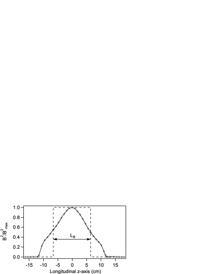
Figure 2: Normalized profile of the square of the magnetic field along the longitudinal z-axis (solid line) inside one Xcoil. This is compared to the equivalent uniform magnetic field (dashed line) over the effective magnetic length L_B (see text).

The pulsed coils are immersed in a liquid nitrogen cryostat to limit the consequences of heating which could be a cause of permanent damage of the coil’s copper wire. Pulse duration is short enough that the coil, starting at liquid nitrogen temperature, always remains at a safe level i.e. below room temperature. A pause between two pulses is necessary to let the magnet cool down to the equilibrium temperature which is monitored via the Xcoils’ resistance. The maximum repetition rate is 5 pulses per hour.

II.3 Fabry-Perot cavity

The other key point of our experiment is to accumulate the effect due to the magnetic field by trapping the light between two ultra high reflectivity mirrors constituting a Fabry-Perot cavity. Its length has to be large enough to leave a wide space so as to insert our two cylindrical cryostats (diameter of 60 cm for each cryostat) and vacuum pumping system. The length of the cavity is $L_{\mathrm{c}}=2.27$ m corresponding to a free spectral range of $FSR=c/2nL{{}_{\mathrm{c}}}\simeq$66 MHz with $n$ the index of refraction of the considered medium in which the cavity is immersed. This index of refraction can be considered equal to one. The total acquired ellipticity $\Psi$ is linked to the ellipticity $\psi$ acquired in the absence of cavity, and depends on the cavity finesse $F$ as follows brandi :

$$\Psi=\frac{2F}{\pi}\psi,$$ (6)

where $F$ is given by:

$$F=\frac{\pi\sqrt{R_{\mathrm{M}}}}{1-R_{\mathrm{M}}},$$ (7)

with $R_{\mathrm{M}}$ the intensity reflection coefficient supposed to be the same for both mirrors. In order to increase the induced signal, a finesse as high as possible is essential.

II.3.1 Cavity finesse and transmission

Experimentally, the finesse is inferred from a measurement of the photon lifetime $\tau$ inside the cavity as presented on Fig 3. For $t<t_{0}$, the laser is locked to the cavity. The laser intensity is then switched off at $t_{0}$ thanks to the AOM shown on Fig. 1 and used as an ultrafast commutator. For $t>t_{0}$, one sees the typical exponential decay of the intensity of the transmitted ordinary beam svelto :

$$I_{\mathrm{t}}(t)=I_{\mathrm{t}}(t_{0})e^{-(t-t_{0})/\tau}.$$ (8)

The photon lifetime is related to the finesse of the cavity through the relation:

$$\tau=\frac{nL_{\mathrm{c}}F}{\pi c}.$$ (9)

By fitting our data with Eq. (8) we get $\tau=1.16$ ms corresponding to a finesse of $F=481\,000$ and a cavity linewidth of $\Delta\nu=c/2nL_{\mathrm{c}}F=137$ Hz.

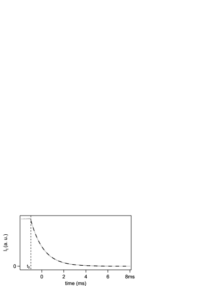
Figure 3: Time evolution of the intensity of the ordinary beam (gray line). The laser is switched off at $t=t_{0}$. Experimental data are fitted by an exponential decay (black dashed line) giving a photon lifetime of $\tau$ = 1.16 ms, a finesse of $F\,=\,481\,000$ and a linewidth of $\Delta\nu\,=\,c/2nL_{\mathrm{c}}F=137$ Hz.

We summarize in Table  1 the performances of some well-known sharp cavities at $\lambda=1064$ nm. To our knowledge, currently our interferometer is the sharpest in the world.

Interferometer	Ref.	$L{{}_{\mathrm{c}}}$(m)	$FSR$(kHz)	$F$	$\tau$($\mu$s)	$\Delta\nu$(Hz)	$Q$
VIRGO	VIRGO	3000	50	50	160	1000	2.8 $\times$ $10^{11}$
TAMA300	TAMA	300	500	500	160	1000	2.8 $\times$ $10^{11}$
PVLAS	PVLAS2008	6.4	23 400	70 000	475	335	8.4 $\times$ $10^{11}$
LIGO	LIGO	4000	37	230	975	163	17 $\times$ $10^{11}$
BMV	this work	2.27	66 000	481 000	1160	137	21 $\times$ $10^{11}$

Table 1: Performances summary of the sharpest infra-red interferometers in the world. $L{{}_{\mathrm{c}}}$ is the length of the Fabry-Perot cavity, $FSR$ is its full spectral range, $F$ is the cavity finesse, $\tau$ is the photon lifetime, $\Delta\nu$ is the frequency linewidth and Q = $\nu_{\mathrm{laser}}/\Delta\nu$ is the quality factor of the interferometer, with $\nu_{\mathrm{laser}}$ the laser frequency.

The transmission of the cavity $T_{\mathrm{c}}$ is another important parameter. It corresponds to the intensity transmitted by the cavity divided by the intensity incident on the cavity when the laser frequency is locked. Indeed in order not to be limited by the noise of photodiodes Ph_t and Ph_e, $I_{\mathrm{t}}$ and $I_{\mathrm{e}}$ have to be sufficiently high. This point is particularly critical for $I_{\mathrm{e}}$ which corresponds to the intensity transmitted by the cavity multiplied by $\sigma^{2}$. With a Ph_e noise equivalent power of 11 fW/$\sqrt{\mathrm{Hz}}$, we need an incident power greater than 0.2 nW so as not to be limited by electronic noise of Ph_e.

Our cavity transmission is 20 $\%$. The measurements of the finesse and the transmission allow to calculate mirrors properties such as their intensity transmission $T_{\mathrm{M}}$ and their losses $P_{\mathrm{M}}$ thanks to the following relations:

$$F = \frac{\pi}{T_{\mathrm{M}}+P_{\mathrm{M}}},$$ (10)

$$T_{\mathrm{c}} = \left(\frac{T_{\mathrm{M}}F}{\pi}\right)^{2},$$ (11)

supposing that the mirrors are identical. We found $T_{\mathrm{M}}=3$ ppm and $P_{\mathrm{M}}=3.5$ ppm, which corresponds to the specifications provided by the manufacturer.

To conclude, our high finesse cavity enhances the Cotton-Mouton effect of a factor $2F/\pi$=306 000, and its transmission allows measurements that are not limited by the noise of the detection photodiodes.

II.3.2 Cavity birefringence

The origin of the total static ellipticity is due to the mirror intrinsic phase retardation. Mirrors can be regarded as wave plates and for small birefringence, combination of both wave plates gives a single wave plate. The phase retardation and the axis orientation of this equivalent wave plate depend on the birefringence of each mirror and on their respective orientations Jacob ; brandi .

The intrinsic phase retardation of the mirrors is a source of noise limiting the sensitivity of the apparatus. Moreover, since our signal detection corresponds to a homodyne technique, the static ellipticity $\Gamma$ is used as a zero frequency carrier. To reach a shot noise limited sensitivity, one needs $\Gamma$ to be as small as possible EPJD_BMV , implying that the phase retardation axis of both mirrors have to be aligned. For magnetic birefringence measurements, both mirrors’ orientation is adjusted in order to have $10^{-3}<\Gamma<3\times 10^{-3}$ rad.

Measurement of the total ellipticity as a function of mirror orientation allows to calculate the mirror intrinsic phase retardation per reflection. The experimental procedure is presented in Ref. BirMirror . The deduced phase retardation for our mirrors is $\delta_{\mathrm{M}}=(7\pm 6)\times 10^{-7}$ rad. Although the origin of the mirrors’ static birefringence is still unknown, a review of existing data shows that for interferential mirrors phase retardation per reflection decreases when reflectivity increases BirMirror . This observation is confirmed by our new measurement. It is also in agrement with the empirical trend given in Ref. BirMirror : $\delta_{\mathrm{M}}\simeq 0.1\times(1-R_{\mathrm{M}})$. Numerical calculations show that this trend can be explained assuming that the effect is essentially due to the layers close to the substrate.

As said before, mirror birefringence has two contributions: one comes from the substrate while the other is due to the reflecting layers. Whereas previous measurements do not allow to distinguish between the two contributions, we will see that this can be achieved with the measurement of $I_{\mathrm{e}}$ decay.

A typical time evolution of $I_{\mathrm{e}}$ when the incident beam locked to the cavity is switched off is shown in Fig.4. We see that this curve can not be fitted by an exponential decay. As explained in Ref. Berceau2010 , one has to take into account the intrinsic birefringence of the cavity. Nevertheless, the expression derived in Ref. Berceau2010 , which only takes into account the reflecting layers birefringence, does not always fit our data. The evolution of $I_{\mathrm{e}}$ presents sometimes an unexpected behavior: whereas no photon enters anymore into the cavity at $t=t_{0}$, the extraordinary intensity starts growing before decreasing. To reproduce this behavior, one has to take into account the substrate birefringence.

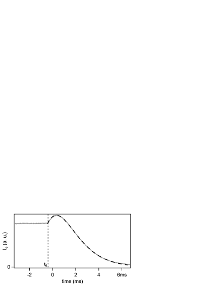
Figure 4: Time evolution of the intensity of the extraordinary beam (gray line). The laser is switched off at $t=t_{0}$. Experimental data are perfectly fitted by Eq. (II.3.2) (black dashed line).

Lets calculate the transmitted intensity along the round-trip inside the cavity:

• For $t\leq t_{0}$, the laser is continuously locked to the cavity. According to Eq. (4), the intensities of the ordinary and the extraordinary beams are related by:

  $$I_{\mathrm{e}}(t\leq t_{0})=[\sigma^{2}+(\Gamma_{\mathrm{s2}}+\Gamma_{\mathrm{s1}}+\Gamma_{\mathrm{c}})^{2}]I_{\mathrm{t}}(t\leq t_{0}).$$ (12)

• At $t=t_{0}$, the laser beam is abruptly switched off, the cavity empties gradually. The ordinary and extraordinary beams are slightly transmitted at each reflection on the mirrors. But, because these mirrors are birefringent, some photons of the ordinary beam are converted into the extraordinary one. The reverse effect is neglected because $I_{\mathrm{e}}\ll I_{\mathrm{t}}$.

We then follow the same procedure as in Ref. Berceau2010 to calculate the time evolution of $I_{\mathrm{e}}$. For $t>t_{0}$, one gets:

$$I_{e}(t)=$$

$$I_{t}(t)\left(\sigma^{2}+\left[\Gamma_{\mathrm{s1}}+\Gamma_{\mathrm{s2}}+\Gamma_{\mathrm{c}}\left(1+\frac{t-t_{0}}{2\tau}\right)\right]^{2}\right).$$

The behavior shown on Fig. 4 is reproduced if $(\Gamma_{\mathrm{s1}}+\Gamma_{\mathrm{s2}})\,\simeq\,-\Gamma_{\mathrm{c}}$.

This expression is used to fit our experimental data plotted on Fig. 4. We find a photon lifetime of $\tau=960\,\mu$s which is in good agreement when fitting $I_{\mathrm{t}}$ It_Ie_justification , $(\Gamma_{\mathrm{s1}}+\Gamma_{\mathrm{s2}})=2\times 10^{-3}$ rad and $\Gamma_{\mathrm{c}}=-7\times 10^{-3}$ rad.

We have for the first time the evidence that the substrate is birefringent and that this birefringence contributes to the total ellipticity due to the cavity.

II.4 Signal analysis

The starting point of our analysis are the voltage signals $V_{\mathrm{e}}$ and $V_{\mathrm{t}}$ provided by Ph_e and Ph_t. Voltage signals have to be converted into intensity signals by using the photodiode conversion factor $g_{\mathrm{e}}$ and $g_{\mathrm{t}}$:

$$I_{\mathrm{e}}=g_{\mathrm{e}}V_{\mathrm{e}},$$ (14)

$$I_{\mathrm{t}}=g_{\mathrm{t}}V_{\mathrm{t}}.$$ (15)

As demonstrated in Ref. Berceau2010 , before analyzing raw signals one has to take into account the first order low pass filtering of the cavity. $I_{\mathrm{t,filtered}}$ in the Fourier space is given by:

$$I_{\mathrm{t,filtered}}(\omega)=\frac{1}{1+i\frac{\omega}{\omega_{\mathrm{c}}}}I_{\mathrm{t}}(\omega),$$ (16)

where $\nu_{\mathrm{c}}=\omega_{\mathrm{c}}/2\pi=1/4\pi\tau$ is the cavity cutoff frequency. Then, according to Eq. (4), the ellipticity $\Psi(t)$ to be measured can be written as:

$$\Psi(t)=-\Gamma+\sqrt{\frac{I_{\mathrm{e}}(t)}{I_{\mathrm{t,filtered}}(t)}-\sigma^{2}}.$$ (17)

The total static birefringence $\Gamma$ is measured a few milliseconds just before the beginning of the magnetic pulse, thus when $\Psi(t)=0$.

On the other hand, $\Psi$ is proportional to the square of the magnetic field and thus can be written as:

$$\Psi(t)=\kappa B^{2}_{\mathrm{filtered}}(t).$$ (18)

Since the photon lifetime is comparable with the rise time of the magnetic field, the first-order low pass filtering of the cavity has also to be taken into account on the quantity $B^{2}(t)$ as in Ref. Berceau2010 . To recover the value of the constant $\kappa$ we calculate for each pulse the correlation between $\Psi(t)$ and $B^{2}_{\mathrm{filtered}}(t)$:

$$\kappa=\frac{\int_{0}^{T_{\mathrm{i}}}\Psi(t)B(t)_{\mathrm{filtered}}^{2}dt}{\int_{0}^{T_{\mathrm{i}}}[B(t)^{2}_{\mathrm{filtered}}]^{2}dt},$$ (19)

where $T_{\mathrm{i}}$ is the integration time. A statistical analysis gives the mean value of $\kappa$ and its uncertainty.

The magnetic birefringence $\Delta n$ is finally given by:

$$\Delta n(T,P)=\frac{\kappa}{4\pi\,\tau\,FSR}\times\frac{\lambda}{L_{B}}\times\frac{1}{\sin 2\theta}.\\$$ (20)

$\Delta n$ is thus expressed in T^-2. $T$ and $P$ correspond to gas temperature and pressure when measurements of magnetic birefringence on gases are performed. We define the normalized birefringence $\Delta n_{\mathrm{u}}$ as $\Delta n$ for $P=1$ atm and $B=1$ T.

III Experimental parameters and error budget

In the following, to evaluate the precision of our apparatus in the present version, we list the uncertainties at 1$\sigma$ on the measurement of the parameters of Eq. (20) as recommended in Ref. CODATA1998 . The uncertainty on the magnetic birefringence has two origins. The evaluation of the uncertainty by a statistical analysis of series of observations is termed a type A evaluation and mainly concerns the measurement of $\tau$ and $\kappa$. An evaluation by means other than the statistical analysis of series of observations, calibrations for instance, is termed a type B evaluation and especially affects the parameters $B$, $FSR$, $L_{B}$, $\lambda$ and $\theta$.

III.1 Photon lifetime in the Fabry-Perot Cavity

The photon lifetime $\tau$ is measured by analyzing the exponential decay of the intensity of the transmitted light. Several measurements have been performed both before and after almost each magnetic pulse. The uncertainty on the value of $\tau$ comes from the fact that mirrors can slightly move because of thermal fluctuations and acoustic vibrations. Measurements conducted in the same experimental conditions have been studied statistically leading to a relative variation of $\tau$ that does not exceed 2 % at 1$\sigma$-level. Data taken during operation, i.e. before and after magnetic pulses, show the same statistical properties as the ones taken without any magnetic field. Thus, the magnetic field does not cause additional change in $\tau$.

III.2 Correlation factor

The correlation factor $\kappa$ is given by Eq. (19). The A-type uncertainty on $\kappa$ depends on the measurement of $\Psi$ and thus on the experimental parameters given in Eq. (17). In practice, we pulse the magnets several times in the same experimental conditions to obtain a set of values of $\kappa$. The distribution of the $\kappa$ values is found to be gaussian, and we assume that its standard deviation corresponds to the A-type uncertainty on $\kappa$. For our measurements performed with nitrogen and presented in section IV.2, the A-type relative uncertainty is typically 3.5 $\%$. The standard uncertainty of the average value of $\kappa$ can then be reduced increasing the number of pulses.

B-type uncertainties depend on those of the square of the magnetic field, the photodiode conversion factors, and the filter function applied to the field.

To measure the magnetic field during operation, we measure the current which is injected in our X-coil. As mentioned in Ref. Batut2008 , the form factor $B/I$ has been determined experimentally during the test phase by varying the current inside the X-coil (modulated at room temperature or pulsed at liquid nitrogen temperature), and by measuring the magnetic field induced on a calibrated pick-up coil. These measurements have led to a relative B-type uncertainty of $\delta B/B$ = 0.7 % for the magnetic field corresponding to a B-type uncertainty on $\kappa$ of 1.4 %.

The ratio $g_{\mathrm{e}}/g_{\mathrm{t}}$ is measured from time to time by sending the same light intensities to each photodiode. The relative uncertainty in this parameter is $1.5$ $\%$ corresponding to the same amount relative uncertainty in $\kappa$.

$I_{\mathrm{t}}$(t) and $B^{2}$(t) are also filtered by a function that involves the parameter $\tau$. We have empirically determined that a $\tau$-variation of 2% led to a $\kappa$-variation of 0.8 %.

We can finally add quadratically the uncertainties above, and deduce that a B-type uncertainty of 2.2 % must be taken into account on every measurement of the correlation factor $\kappa$.

III.3 Frequency splitting between perpendicular polarizations

In this section we evaluate the attenuation of the extraordinary beam transmitted by our sharp resonant Fabry-Perot cavity on which the laser’s ordinary beam is frequency-locked. Let’s suppose that the ordinary (resp. extraordinary) beam resonates in the interferometer at the frequency $\nu_{\mathrm{t}}$ (resp. $\nu_{\mathrm{e}}$). The laser is locked to the cavity thanks to the ordinary beam. Thus $\nu_{\mathrm{t}}$ corresponds to the top of the transmission Airy function A of the Fabry-Perot cavity which is given by:

$$\emph{A}(\nu)=\frac{T_{\mathrm{c}}}{1+\frac{4F^{2}}{\pi^{2}}\sin^{2}\big{(}\frac{2\pi nL_{\mathrm{c}}}{c}\nu\big{)}}.$$ (21)

The frequency $\nu_{\mathrm{e}}$ is shifted from $\nu_{\mathrm{t}}$ by a quantity $\delta\nu$ as it is shown on Fig. 5.

Figure 5: Airy function of our Fabry-Perot cavity (linewidth $\Delta\nu$ = 137 Hz and transmission $T_{\mathrm{c}}$ = 20 %). The frequency of the ordinary beam is assumed to be locked at the top of the transmission function (solid line) while he frequency $\nu_{\mathrm{e}}$ of the extraordinary beam is shifted from $\nu_{\mathrm{t}}$ of a quantity $\delta\nu$ (dashed line).

The frequency splitting $\delta\nu=\nu_{\mathrm{t}}-\nu_{\mathrm{e}}$ can be expressed as a function of the phase retardation $\delta$ acquired along a round-trip between the ordinary and the extraordinary beams:

$$\delta\nu = \frac{c}{2\pi nL_{\mathrm{c}}}\delta,$$ (22)

$$= \frac{F\Delta\nu}{\pi}\delta.$$

This formula indicates that in order to have a splitting very small compared to the cavity linewidth ($\delta\nu\,\ll\,\Delta\nu$), the phase retardation $\delta$ must satisfy the following condition:

$$\delta\ll\frac{\pi}{F},$$ (23)

which is equivalent to the condition on the acquired total ellipticity $\Psi$:

$$\Psi\ll 1.$$ (24)

By combining Eqs. (21) and (22), we obtain the factor of attenuation a of the transmitted extraordinary beam’s intensity given by:

a $$= \frac{\emph{A}(\nu_{\mathrm{e}})}{\emph{A}(\nu_{\mathrm{t}})},$$ (25)

$$= \frac{1}{1+\frac{4F^{2}}{\pi^{2}}\sin^{2}\big{(}\frac{2\pi nL_{\mathrm{c}}}{c}\delta\nu\big{)}},$$

$$= \frac{1}{1+\frac{4F^{2}}{\pi^{2}}\sin^{2}\big{(}\delta\big{)}}.$$

The attenuation factor a is plotted as a function of $\delta$ on Fig. 6 for a finesse $F$ = 481 000. The real intensity $I_{\mathrm{e}}$ of the extraordinary beam transmitted by the cavity is obtained from the corrected measured intensity $I_{\mathrm{e}}^{\mathrm{meas}}$ as $I_{\mathrm{e}}\,=\,I_{\mathrm{e}}^{\mathrm{meas}}\,/\,\emph{a}$.

Figure 6: Attenuation factor a as a function of the phase retardation $\delta$ between both polarizations.

The frequency splitting can first be due to our birefringent cavity. As in Ref. brandi , let’s consider both cavity mirrors equivalent to a single wave-plate with phase retardation $\delta_{\mathrm{w}}=\delta$ between both polarizations. The total phase retardation $\delta_{\mathrm{w}}$ is linked to the cavity mirrors’ M₁ and M₂ own phase retardation $\delta_{1}$ and $\delta_{2}$ as brandi :

$$\delta_{\mathrm{w}}=\sqrt{(\delta_{1}-\delta_{2})^{2}+4\delta_{1}\delta_{2}\cos^{2}(\theta_{\mathrm{m}})}.$$ (26)

To set a $\delta_{\mathrm{w}}$ as small as possible so as to minimize the correction to $I_{\mathrm{e}}^{\mathrm{meas}}$, one needs to adjust the angle $\theta_{\mathrm{m}}$ between the neutral axes of both mirrors. This way, we set a $\delta_{\mathrm{w}}$ of the order of a few $10^{-8}$ rad, corresponding to a correction smaller than 0.001 % on $I_{\mathrm{e}}^{\mathrm{meas}}$.

Secondly, the frequency splitting between both polarizations can be due to the induced magnetic birefringence of the medium inside the chamber. As seen above, the induced ellipticity given by Eq. (24) must be well below 1 rad. This condition is always satisfied in the range of pressure and field we are working. The induced ellipticity does not exceed $10^{-2}$ rad. This corresponds at worst to a phase retardation of $\delta$ = $10^{-7}$ rad. The attenuation factor $I_{\mathrm{e}}^{\mathrm{meas}}$ is thus smaller than 0.1 $\%$.

In principle, this attenuation generates an error that has to be taken into account in the measured ratio $I_{\mathrm{e}}/I_{\mathrm{t,filtered}}$ of Eq. (17), which implies an error in the value of $\kappa$. At present, since the attenuation is smaller than 0.1 %, this error can be neglected compared to the others uncertainties in $\kappa$.

III.4 Cavity free spectral range

The dedicated experimental setup for the measurement of the cavity free spectral range $FSR=c/2nL_{\mathrm{c}}$ is shown on Fig. 7. The principle is to inject into the cavity two laser beams shifted one compared with the other by a given frequency. This frequency is then adjusted to coincide with the free spectral range.

Experimentally, the main beam is divided into two parts thanks to a polarizing beam splitting cube. The first part is directly injected into the cavity while the other one is frequency shifted by the acousto-optic modulator AOM2 with a double-pass configuration before injection. The main beam is frequency modulated with a voltage ramp applied on a piezo element mounted on the crystal resonator of the laser.

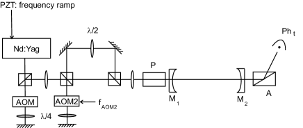
Figure 7: Experimental setup for the cavity length measurement. Two laser beams frequency shifted one compared to the other by AOM2 are injected into the cavity. The frequency of the laser is frequency modulated with a voltage ramp applied on a piezo element mounted on the crystal resonator of the laser. Photodiode Ph_t allows to observe the typical Fabry-Perot peaks from which the $FSR$ measurement is performed.

The intensity transmitted by the cavity is observed on Ph_t as shown on Fig. 8. The solid line corresponds to the intensity of the first beam. We observe typical Fabry-Perot peaks whose frequency gap corresponds to $FSR$. Peaks due to the second beam (dashed line) are frequency shifted by $2f_{\mathrm{AOM2}}$. We finally adjust $f_{\mathrm{AOM2}}$ in order to superimpose both series of peaks. The precise knowledge of the driven frequency $f_{\mathrm{AOM2}}$ enables us to determine with the same precision the value of the free spectral range, and thus the cavity length.

Figure 8: Transmission peaks of the Fabry-Perot cavity as a function of the laser frequency. Two beams are sent to the interferometer: the second beam (dashed line) is frequency shifted by $2f_{\mathrm{AOM2}}$ compared to the first beam (solid line). The adjustment of $f_{\mathrm{AOM2}}$ in order to superimpose both series of peaks allows to precisely measure the free spectral range $FSR$ of the cavity.

A typical value is $FSR=(65.996\pm 0.017)$ MHz. This corresponds to a cavity length of $L_{\mathrm{c}}=(2.2713\pm 0.0006)$ m. Since this length can be prone to variation, the $FSR$ value is regularly checked and updated.

III.5 Effective magnetic length

Following Eq. (5), the effective magnetic length $L_{B}$ has been calculated by numerically integrating the field measured with a calibrated pick-up coil. Taking into account the experimental uncertainties, we got for one Xcoil: $L_{B}$ = (0.137 $\pm$ 0.003) m, corresponding to a relative B-type uncertainty on $L_{B}$ of 2.2 %.

III.6 Laser wavelength

As mentioned above, infra-red light enters the cavity. The wavelength of the Nd:YAG laser is 1064 nm, and its uncertainty is given by the width of the laser transition. The natural linewidth of Nd:YAG lasers are not usually given by the manufacturers. However, we can estimate it from the bandwidth of the gain curve of the amplifying medium. It is typically of the order of 30 GHz Hecht . This corresponds to an uncertainty on the laser wavelength of 0.3 nm. In order to be conservative, we use $\lambda=(1064.0\pm 0.5)$ nm. The relative uncertainty is negligible in our case, compared to main uncertainties.

III.7 Angle between the incident polarization and the magnetic field direction

The angle between the incident light polarization and the magnetic field direction is adjusted to $45\textdegree$ thanks to magnetic birefringence measurements as a function of the polarizer direction $\theta_{\mathrm{P}}$. In order to be more sensitive, this is performed close to the position where the magnetic field is parallel to the polarizer P ($\theta=0\textdegree$).

Measurements are realized with about 7$\,\times\,10^{-3}$ atm of air. The analyzer direction is crossed at maximum extinction each time the polarizer is turned. Fig. 9 represents the evolution of the correlation factor $\kappa$ as a function of $\theta_{\mathrm{P}}$. Data are fitted by a sinusoidal trend $\kappa(\theta_{\mathrm{P}})=\kappa_{0}\sin\bigl{[}2(\theta_{\mathrm{P}}-\theta_{0})\bigr{]}$ giving $\theta_{0}=(2.6\pm 0.2)\textdegree$. This measurement allows to set $\theta$ to $(45.0\pm 1.2)\textdegree$. The uncertainty is mainly due to the mechanical system which holds and turns the polarizer.

Figure 9: Correlation factor $\kappa$ between the square of the magnetic field and the ellipticity as a function of the angle $\theta_{\mathrm{P}}$ of the incident polarization.

III.8 Error budget

We summarize in the Table 2 the typical values of the experimental parameters that have to be measured and their B-type associated uncertainty. These uncertainties are quadratically added to give a B-type relative uncertainty on the birefringence $\Delta n$ of 3.1 % at 1$\sigma$.

Parameter	Typical	Relative
	value	B-type uncertainty
$\kappa$	$10^{-5}$ rad T-2	$2.2\times 10^{-2}$
$FSR$	65.996 MHz	$3\times 10^{-4}$
$L_{B}$	0.137 m	$2.2\times 10^{-2}$
$\lambda$	1064.0 nm	$<$ $5\times 10^{-4}$
$\sin 2\theta$	1.0000	$9\times 10^{-4}$
total		$3.1\times 10^{-2}$

Table 2: Parameters that have to be measured to infer the value of the birefringence $\Delta n$ and their respective relative B-type uncertainty at 1$\sigma$.

III.9 Temperature and pressure of gases

Gas magnetic birefringence measurements are performed at room temperature $T\,$= 293 K. The experimental room is air-conditioned. A flow of compressed air between the outer wall of the vacuum pipe and the liquid nitrogen cryostat containing the magnet maintains the room temperature in the gas chamber.

A temperature profile has been realized along the length of the vacuum pipe, and is plotted on Fig. 10. The temperature variation does not exceed 1 K inside the tube that passes through the magnetic field. Concerning gases, we consider that our birefringence measurements are given at (293 $\pm$ 1) K.

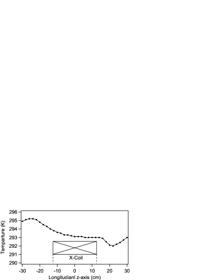
Figure 10: Profile of the temperature inside the vacuum pipe along the longitudinal z-axis. The X-coil is also schematized at the center. The temperature variation does not exceed 1 K inside the tube that runs through it.

The pressure of the gas inside the chamber is measured at each side of the vacuum pipe getting into magnets with pressure gauges. The relative uncertainty provided by the manufacturer is 0.2 %.

IV Magnetic birefringence measurements

IV.1 Raw signals

Fig. 11 presents signals obtained with 32.1$\,\times\,10^{-3}$ atm of molecular nitrogen. The intensity of the ordinary beam $I_{\mathrm{t}}$ (top) remains almost constant while the intensity of the extraordinary beam $I_{\mathrm{e}}$ (middle) varies when the magnetic field (bottom) is applied. The magnetic field reaches its maximum of 5.2 T within less than 2 ms.

The laser beam remains locked to the Fabry-Perot cavity, despite mechanical vibrations caused by the shot of magnetic field. $I_{\mathrm{t}}$ and $I_{\mathrm{e}}$ start oscillating after about 4 ms. Seismometers placed on mirror mounts show that these oscillations are mainly due to acoustic perturbations produced by the magnet pulse and propagating from the magnet to mirror mounts through the air. We also see that the minimum of $I_{\mathrm{e}}$ does not coincide with the maximum of $B^{2}$. This phenomenon is due to the cavity filtering as explained in details in Ref. Berceau2010 .

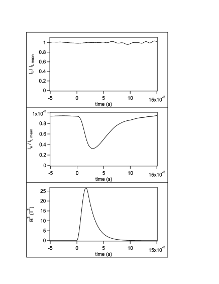
Figure 11: Cotton-Mouton effect measurement on 32.1$\,\times\,10^{-3}$ atm of molecular nitrogen. (top) Normalized intensity of the ordinary beam as a function of time. (middle) Intensity of the extraordinary beam divided by the mean of $I_{\mathrm{t}}$ as a function of time. (bottom) Square of the magnetic field as a function of time.

In Fig. 12, we plot the square of the magnetic field filtered by the cavity and the ellipticity calculated with Eq. (17) as a function of time. Since the acoustic perturbations affect both signals $I_{\mathrm{t}}$ and $I_{\mathrm{e}}$, and taking into account the cavity filtering between $I_{\mathrm{t}}$ and $I_{\mathrm{e}}$, oscillations on $\Psi$ are strongly reduced to a few $10^{-5}$ rad, thus not visible on this figure. These oscillations induce uncertainty to the measurement but are already included in the A-type uncertainty on kappa measured in section III.2.

Finally, we note that both quantities $B^{2}_{\mathrm{filtered}}$ and $\Psi$ reach their extremum at the same time and their variation can be perfectly superimposed, providing a very precise measurement of magnetic linear birefringence of nitrogen gas.

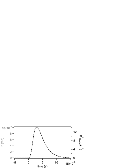
Figure 12: Cotton-Mouton effect measurement on 32.1$\,\times\,10^{-3}$ atm of molecular nitrogen. Gray line: Total ellipticity as a function of time. Dashed line: Square of the magnetic field filtered by a first-order low pass filter corresponding to the cavity filtering.

IV.2 Apparatus calibration

In order to calibrate our apparatus and to evaluate its present sensitivity we have measured the magnetic birefringence of molecular nitrogen. These measurements have been performed at different pressure from 2.1$\,\times\,10^{-3}$ to 32.1$\,\times\,10^{-3}$ atm and are summarized in Fig. 13.

Figure 13: Magnetic birefringence of molecular nitrogen as a function of pressure. The solid line corresponds to the linear fit of experimental data.

In this range, nitrogen can be considered as an ideal gas and the pressure dependence of its birefringence is thus linear:

$$\Delta n(\mathrm{T}^{-2})=\Delta n_{\mathrm{u}}(\mathrm{atm}^{-1}\mathrm{T}^{-2})\times P(\mathrm{atm}).$$ (27)

We have checked that our data are correctly fitted by a linear equation. Its $\Delta n$ axis-intercept is consistent with zero within the uncertainties. Its slope gives the normalized magnetic birefringence at $B=1$ T and $P=1$ atm:

$$\Delta n_{\mathrm{u}}=(-2.00\pm 0.08\pm 0.06)\times 10^{-13}\,\mathrm{atm}^{-1}\mathrm{T}^{-2}.$$

The first uncertainty $0.08\times 10^{-13}$ atm^-1T^-2 corresponds to the fitting uncertainty and represents the A-type total uncertainty at 1$\sigma$. The second one $0.06\times 10^{-13}$ atm^-1T^-2 represents the B-type uncertainty at 1$\sigma$.

Our value of the normalized birefringence is compared in Table. 3 to other experimental published values at $\lambda=1064$ nm Bregant2004 ; QandA . This shows that our value agrees perfectly well with other existing measurements. Our total uncertainty is $10^{-14}$ atm^-1T^-2, calculated by quadratically adding the A-type and B-type uncertainties. This is 1.8 times more precise than the other results. It therefore provides a successful calibration of the whole apparatus.

Ref.	$\Delta n_{\mathrm{u}}\times 10^{-13}$
	(at $P$ = 1atm and $B$ = 1T)
Bregant2004	-2.17 $\pm$ 0.21
QandA	-2.02 $\pm$ 0.16 $\pm$ 0.08
This work	-2.00 $\pm$ 0.08 $\pm$ 0.06

Table 3: Comparison between our value of the nitrogen normalized magnetic birefringence and other experimental published values at $\lambda=1064$ nm.

IV.3 Upper limit on vacuum magnetic birefringence measurements

Once the calibration performed we have evaluated the upper limit of the present apparatus on vacuum magnetic birefringence. To this end, several pulses were performed in vacuum. In Fig. 14, a typical ellipticity measured during a magnetic pulse is plotted. Acoustic perturbations induce oscillations of $\Psi$ starting at about 4 ms, with variations of the order of $10^{-5}$ rad. In order to infer our best upper limit for the value of the vacuum magnetic birefringence, we limit the integration time to 4 ms. We get $\Delta n\,<\,5.0\,\times\,10^{-20}$ T^-2 per pulse.

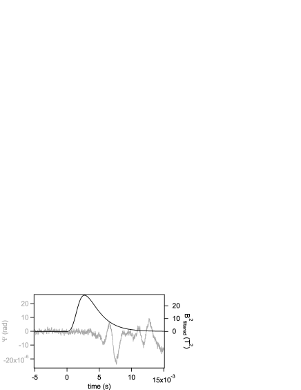
Figure 14: Typical ellipticity (gray) measured during a magnetic pulse (black) performed in vacuum. Acoustic perturbations generate ellipticity oscillations starting at 4 ms.

During operation, the pressure inside the UHV system was better than $10^{-10}$ atm. To be conservative, lets assume residual gases are mainly 78 % of nitrogen and 21 % of oxygen. The normalized magnetic birefringences of these gases are of the order of $-2\times 10^{-13}\,\mathrm{atm}^{-1}\mathrm{T}^{-2}$ and $-2\times 10^{-12}\,\mathrm{atm}^{-1}\mathrm{T}^{-2}$ respectively Rizzo1997 . The total residual magnetic birefringence is then of the order of $6\times 10^{-23}\,\mathrm{T}^{-2}$, which is well below our current upper limit. In the final setup, vacuum quality will be monitored with a residual gas analyzer.

V Conclusion

The successful calibration we report in this paper is a crucial step towards the measurement of the vacuum magnetic birefringence. It shows our capability to couple intense magnetic fields with one of the sharpest Fabry-Perot cavity in the world. It is worthwhile to note that an energy of about 100 kJ is discharged in our coils during a few milliseconds. These 10 MW of electrical power generate acoustic perturbations and mechanical vibrations that tend to misalign the cavity mirrors. The linewidth $\Delta\nu$ of our Fabry-Perot cavity is of the order of 150 Hz. A relative displacement $\Delta L_{c}=L_{c}\times\Delta\nu/\nu_{\mathrm{laser}}$ = 1 pm of both mirrors is enough to get out of resonance. The sharper the cavity, the bigger the challenge.

The sensitivity per pulse we got both in gases and in vacuum is the best ever reached for this kind of measurement. For sake of comparison, the best birefringence limit obtained in vacuum with continuous magnets is $\Delta n\,\leq\,2.1\,\times\,10^{-20}$ $\mathrm{T}^{-2}$ with an integration time of $t_{\mathrm{int}}$ = 65 200 s PVLAS2008 . In order to compare both methods, we need to translate the best limit obtained in continuous regime to the one obtained with our integration time $T_{\mathrm{i}}$ = 4 ms. Assuming white noise for both methods, best limit reported in Ref. PVLAS2008 corresponds to $\Delta n(T_{\mathrm{i}})=\Delta n(t_{\mathrm{int}})\sqrt{t_{\mathrm{int}}/T_{\mathrm{i}}}\leq\ 8.5\,\times\,10^{-17}$ in 4 ms of integration. This value is more than three orders of magnitude higher than ours, proving that pulsed fields are a powerful tool for magnetic birefringence measurements.

Long terms perspective is to get a value of $\Delta n=4\,\times\,10^{-24}\mathrm{T}^{-2}$, corresponding to the vacuum magnetic birefringence, with at most 1000 pulses. This corresponds to a sensitivity better than $1.3\,\times\,10^{-22}\mathrm{T}^{-2}$ per pulse. A factor of the order of 10 on optical sensitivity will be achievable with a better acoustic insulation and a more robust locking system, especially reducing the noise of the measured light intensities transmitted by the cavity. Further improvements depend on the possibility to have higher magnetic fields. We have designed a new pulsed coil, called XXL-coil, which has already reached a field higher than 30 T when a current higher than 27 000 A is injected. This corresponds to more than 300 T²m sitewebLNCMI . Two XXL-coils will allow us to improve our current sensitivity by a factor 100. In the near future, the apparatus will be modified in order to host these XXL-coils. Therefore the final version of the experiment will be ready for operation.