Electron transport through a coupled double dot molecule: role of inter-dot coupling, phononic and dissipative effects

Abstract

In this work, we have investigated conduction through an artificial molecule comprising two coupled quantum dots. The question addressed is the role of inter-dot coupling on electronic transport. We find that the current through the molecule exhibits step-like features as a function of the voltage between the leads, where the step size increases as the inter-dot coupling is increased. These step-like features disappear with increasing tunneling rate from the leads, but we find that in the presence of coupling, this smooth behavior is not observed rather two kinks are seen in the current voltage curve. This shows that the resolution of the two levels persists if there is finite inter-dot coupling. Furthermore, we also consider the effects of electron-phonon interaction as well as dissipation on conduction in this system. Phononic side bands in the differential conductance survive for finite inter-dot coupling even for strong lead to molecule coupling.

year number number identifier Date text]date

LABEL:FirstPage1 LABEL:LastPage#12

.1 Introduction

Ever since the original proposal of a single molecule rectifying diode by A. Aviram and M. A. Ratner1 , there has been great interest in electron transport (both charge and spin) at the single molecule level. Theoretical as well as experimental work in this direction has led to the promising field of molecular electronics6 8 . With an eye on applications it is expected that the understanding of quantum electron transport at the molecular scale is a key step to realizing molecular electronic devices3 . Experiments on conduction in molecular junctions are becoming more common, 4 5 and references therein. On the experimental front, the most common methods of contacting individual molecules are through scanning tunneling microscope tips and mechanically controlled break junctions 6 8 . Early experiments focused on the absolute conduction and on trends such as dependence on wire length, molecular structure, and temperature. From a theoretical point of view, investigating electron transport in an electrically contacted molecule is a challenging problem. In this system, the interaction of the electronic degrees of freedom with the vibrational ones of the molecule need to be considered. In addition, there can be further complications arising from the electron-electron interaction on the molecule as well as effects of the environment surrounding the system. Most of the formal theoretical work on transport in molecular electronics has relied on the generalized master equations approach 9 10 and the non equilibrium Green’s function (NEGF) method7 .

As mentioned above, an important feature that can affect charge transport in a single molecule is the coupling of electrons to quantized molecular vibrational motion, phonons 19 20 . For transport through a single level quantum dot molecule a lot of work has already been done taking into account vibrational degrees of freedom11 12 13 . In this paper, we consider transport through a single molecule consisting of two coupled quantum dots in parallel configuration. Electron transport in double quantum dots has been an area of active research, 34 and references therein. In parallel configuration electron from the lead can tunnel through either of the two dots. We address the role of finite coupling between the dots on the electronic transport. We also take into account the electron-phonon interaction as well as the dissipative effects of the environment. It has been established that it is important to take into account electron-phonon interaction in the study of transport in single and double dot systems35 . Here we show that the inter-dot coupling will significantly affect transport when a single electron can occupy either dot in the presence of electron-phonon interaction. The difference in the transport properties with and without inter-dot coupling will be discussed in detail in this work. For a single level molecular system with electron phonon interaction, phonon side band peaks start disappearing with increasing tunneling rate2 whereas we find that for a coupled dot molecule the phonon peaks survive even if the tunneling rate from the leads is increased.

.2 Model

Our system is a laterally coupled double quantum dot. It is assumed that only a single level in each dot participates in transport. We allow finite coupling between the single electronic levels of the two dots. An electron from the leads can tunnel through either of the two dots.

The full Hamiltonion describing our system is

$$H=H_{M}+H_{Leads}+H_{T}.$$

It is the sum of the electron Hamiltonian of the coupled dot molecule $H_{M}$, the Hamiltonian of the leads $H_{Leads}$, the tunneling Hamiltonian $H_{T}$ describing the molecule-to-lead coupling. We explain each term in the full Hamiltonian separately:

$$H_{M}=\sum_{i=1,\sigma}^{2}\epsilon_{i\sigma}d_{i\sigma}^{{\dagger}}d_{i\sigma}+\sum_{i,j=1i\neq j,\sigma}^{2}t_{i,j,\sigma}d_{i\sigma}^{{\dagger}}d_{j\sigma}.$$ (1)

The first term represents two discrete energy levels, one in each dot. $d_{i\sigma}^{{\dagger}},$ $d_{i\sigma}$ create and annihilate an electron in state $|i\sigma>$ on the dot. The second term represents inter-dot coupling where $t_{i,j,\sigma}$ represents coupling between the electronic states of the two dots. We have assumed $t_{i,j,\sigma}=t_{j,i,\sigma}=t$.

$$H_{Leads}=\sum_{k}\epsilon_{\nu k\sigma}c_{\nu k\sigma}^{{\dagger}}c_{\nu k\sigma}.$$ (2)

This represents the leads Hamiltonian. Indices $\nu,k,\sigma$ refer to the left/right leads, the electronic wave vector in either lead, and leads electrons spin.

The tunneling Hamiltonian describes hopping between the leads and the molecule. Direct hopping between the two leads is neglected:

$$H_{T}=\sum_{i,k}(V_{i,\nu,k,\sigma}c_{\nu k\sigma}^{{\dagger}}d_{i\sigma}+hc).$$ (3)

The first term represents creation of electrons in the lead and annihilation of electrons in the coupled dots, while the second term represents creation of electrons in the coupled dots and annihilation in the lead. Here $V_{i,\nu,k,\sigma}$ denotes lead-system coupling (hopping) amplitude and $hc$ denotes hermitian conjugation. We consider contacting the coupled dots with two metallic leads.

Finally, phonons, electron-phonon coupling, heat bath and phonons coupling are described by the following Hamiltonian17 (In this calculation we work with $\hbar=1$):

$$H_{phonon+Bath} =\sum_{q}\omega_{q}a_{q}^{{\dagger}}a_{q}+\sum_{\alpha=1}^{2}\sum_{q}\lambda_{\alpha\alpha}^{q}(a_{q}^{{\dagger}}+a_{q})d_{\alpha}^{{\dagger}}d_{\alpha}+$$

$$\sum_{\beta}\omega_{\beta}b_{\beta}^{{\dagger}}b_{\beta}+\sum_{q\beta}N_{q\beta}(b_{\beta}^{{\dagger}}+b_{\beta})(a_{q}^{{\dagger}}+a_{q}).$$ (4)

The electron-phonon interaction is included with in the first Born approximation, which is resonable when electron phonons coupling is weak. For a single dot molecule this problem was studied in 21 22 , whereas we consider two dots in the molecule interacting with phonons of frequency $\omega_{q}$. The first and the third term represents phononic and heat bath energy. Here $\omega_{q}$, $\omega_{\beta}$ are phonon and heat bath energies. $a_{q}^{{\dagger}}a_{q}(b_{\beta}^{{\dagger}}b_{\beta})$ are phonons creation and annihilation operators (heat bath creation and annihilation operators). The second term represents electron-phonon interaction and $\lambda_{\alpha\alpha}^{q}$ is the coupling strength of this interaction. The last term represents phonon and heat bath coupling and $N_{q\beta}$ is the coupling strength of phonon heat bath interaction.

.3 Method

Our approach is based on the nonequilibrium Green function technique29 30 , which is now a standard technique in mesoscopic physics as well as molecular electronics. We follow the formulation pioneered by Meir and Wingreen31 , Jauho and co-workers14 33 . The case of intermediate and strong electron-phonon coupling at finite tunneling rates is the most interesting regime but it is also the most difficult. Only the approaches by Flensberg24 . and Galperin et al17 exist, both starting from the exact solution for the isolated system and then switching on tunneling as a perturbation2 .The current from lead $\nu$ is given by the well known expression32

$$J^{\nu}(\epsilon) =\frac{e}{2\pi}\sum_{i,j,k}\int_{-\infty}^{\infty}d\epsilon[\{G_{ij}^{r}(\epsilon)-G_{ij}^{a}(\epsilon)\}\Sigma_{ji\nu k}^{<}(\epsilon)+$$ (5)

$$G_{ij}^{<}(\epsilon)\{\Sigma_{ji\nu k}^{a}(\epsilon)-\Sigma_{ji\nu k}^{r}(\epsilon)\}].$$

Here $\Sigma_{ji\nu k}^{<,r,a}$ represents lesser, retarded and advanced self energies of leads and coupled dot molecule. $\Sigma_{ji,\nu}^{<,r,a}=\sum_{k}\{V_{j\nu k}^{{\dagger}}g_{\nu}^{<,r,a}(\epsilon)V_{i\nu k}\}$ where $g_{\nu}^{<,r,a}(\epsilon)$ is the lesser,retarded and advanced Green’s function of the leads.31 .

We employ the wide-band approximation, where the self-energy of the coupled dot molecule due to each lead is taken to be energy independent and is given by

$$\sum_{k}\Sigma_{ji\nu k}^{r,a}(\epsilon)=DV_{i\nu k}V_{j\nu k}^{{\dagger}}\int_{-\infty}^{\infty}\dfrac{d\epsilon_{k}}{(\epsilon-\epsilon_{k}\pm i\eta)}\qquad\eta\rightarrow 0^{\mp}=-i2\pi D(\epsilon_{\nu})V_{i\nu k}V_{j\nu k}^{{\dagger}}=\mp i\dfrac{\Gamma_{ji}^{\nu}}{2}.$$

Here $D$ is the constant energy density of the leads. Similiarly the lesser self energy can be written as

$$\sum_{k}\Sigma_{ji\nu k}^{<}(\epsilon)=i\Gamma_{ji}^{\nu}f(\epsilon)$$ (6)

where $\Gamma_{ji}^{\nu,}s$ are the tunneling rates (coupling of leads with the molecule) and $f(\epsilon)$ is the Fermi-Dirac distribution function.

Now by employing the current symmetrization and line width proportionality approximations14 we obtain

$$J^{\nu}(\epsilon)=\frac{ie}{2\pi}\sum_{i,j}\left(\frac{\Gamma_{ji}^{L}\Gamma_{ji}^{R}}{\Gamma_{ji}^{L}+\Gamma_{ji}^{R}}\right)\int_{-\infty}^{\infty}d\epsilon[\{G_{ij}^{r}(\epsilon)-G_{ij}^{a}(\epsilon)\}\{f^{L}(\epsilon)-f^{R}(\epsilon)\}].$$ (7)

By using the equation of motion technique, we work out the coupled dot molecule Green’s function and find

$$(g_{ii}^{r}(\epsilon))^{-1}=\left(\epsilon-\epsilon_{i}-\frac{\mid t_{i,j}\mid^{2}}{\epsilon-\epsilon_{j}}\right)\qquad i\neq j.$$ (8)

$$(g_{i,j}^{r}(\epsilon))^{-1}=\frac{\left(\epsilon-\epsilon_{j}\right)}{t_{j,i}}\left(\epsilon-\epsilon_{i}-\frac{\mid t_{i,j}\mid^{2}}{\epsilon-\epsilon_{j}}\right)\qquad i\neq j$$ (9)

Employing Dyson’s equation, we can write

$$G_{ij}^{r}(\epsilon)=\left[(g_{ij}^{r}(\epsilon))^{-1}-\Sigma_{ji\nu k}^{r}(\epsilon)\right]^{-1}.$$ (10)

The differential conductance in the absence of electron-phonon interaction is

$$\frac{dJ^{\nu}}{dV}=\frac{e^{2}}{2\pi}\sum_{i,j}\left[\dfrac{\Gamma_{ji}^{L}\Gamma_{ji}^{R}}{\left((g_{ij}^{r}(\epsilon))^{-1}\right)^{2}+\left(\dfrac{\Gamma_{ji}^{L}+\Gamma_{ji}^{R}}{2}\right)^{2}}\right].$$ (11)

If the electron-phonon interaction is included then our total self energy will become

$$\Sigma_{Total}=\Sigma_{Leads}+\Sigma_{el+phonon}.$$

and in the Hartree-Fock approximation

$$\Sigma_{el+ph}=\Sigma_{Hartree}+\Sigma_{Fock}$$ (12)

where

$$\Sigma_{ji,Hartree}^{r}(\epsilon)=-i\sum_{q}\lambda_{q}^{2}\int_{-\infty}^{\infty}\frac{d\epsilon}{2\pi}D_{0}^{r}(q,\epsilon=0)G_{ji}^{<}(\epsilon)$$ (13)

and

$$\Sigma_{ji,Fock}^{r}(\epsilon) =-i\sum_{q}\lambda_{q}^{2}\int_{-\infty}^{\infty}\frac{d\epsilon^{\prime}}{2\pi}\left[D_{0}^{r}(q,\epsilon-\epsilon^{\prime})G_{ji}^{<}(\epsilon^{\prime})+\right.$$

$$\left.D_{0}^{r}(q,\epsilon-\epsilon^{\prime})G_{ji}^{r}(\epsilon^{\prime})+D_{0}^{<}(q,\epsilon-\epsilon^{\prime})G_{ji}^{r}(\epsilon^{\prime})\right].$$ (14)

Here $D_{0}^{r,<}$ represents retarded and lesser free phonon Green’s function. At this stage if we also include the effects of the heat bath then our zeroth order phonon Green’s function will be

$$D_{0}^{r}(\epsilon,\omega_{q})=\dfrac{1}{\epsilon-\omega_{q}+\dfrac{i\gamma}{2}}-\dfrac{1}{\epsilon+\omega_{q}+\dfrac{i\gamma}{2}}$$ (15)

with $\gamma=2\pi\sum_{\beta}|N_{q\beta}|^{2}\delta(\epsilon-\omega_{\beta})$, 17 , represents dissipation in phonon energy due to its contact with the heat bath.

$$D_{0}^{<}(\epsilon)=-in(\epsilon)\dfrac{\gamma}{(\epsilon-\omega_{q})^{2}+\left(\dfrac{\gamma}{2}\right)^{2}}-i(1+n(\epsilon))\dfrac{\gamma}{(\epsilon+\omega_{q})^{2}+\left(\dfrac{\gamma}{2}\right)^{2}}$$ (16)

with $n(\epsilon)$ the Bose-Einstein distribution function. At zero temperature the imaginary part of the electron-phonon self energy is

$$\text{Im}\Sigma_{ji,el+phonon}=\frac{1}{2}\sum_{q}\lambda_{q}^{2}[A_{ji}(z-\omega_{q})-A_{ji}(z+\omega_{q})]$$ (17)

where the spectral function $A_{ji}(\epsilon)=-2\operatorname{Im}G_{ji}^{r}(\epsilon),$ whereas

$$\operatorname{Re}\Sigma_{ji,el+phonon}=\sum_{q}\lambda_{q}^{2}\left[\operatorname{Re}G_{ji}^{r}(z-\omega_{q})-\operatorname{Re}G_{ji}^{r}(z+\omega_{q})+\dfrac{1}{2\omega_{q}}\right]$$ (18)

with

$$z\longrightarrow\epsilon+\frac{i\gamma}{2}.$$ (19)

In the presence of electron-phonon interaction and the dissipative effects of the heat bath, the differential current is

$$\frac{dJ^{\nu}}{dV}=\frac{e^{2}}{2\pi}\sum_{i,j}\dfrac{\Gamma_{ji}^{L}\Gamma_{ji}^{R}}{\Gamma_{ji}^{L}+\Gamma_{ji}^{R}}\dfrac{\left(\Gamma_{ji}^{L}+\Gamma_{ji}^{R}+Im\Sigma_{ji,el+phonon}\right)}{\left((g_{ij}^{r}(\epsilon))^{-1}+\operatorname{Re}\Sigma_{ji,el+phonon}\right)^{2}+\left(\genfrac{}{}{1.0pt}{0}{\Gamma_{ji}^{L}+\Gamma_{ji}^{R}}{2}+Im\Sigma_{ji,el+phonon}\right)^{2}}$$ (20)

.4 Results And Discussions

The system under consideration is a molecule comprising two coupled quantum dots. This molecule is attached to two metallic leads. The primary focus of this study is the role of inter-dot coupling in electronic transport. In addition, the dissipative effects of the environment is taken into account by treating the transport in this system surrounded by a heat bath of phonons. The vibrational states of the molecule and its impact on electronic transport is included through the electron-phonon interaction. Our results show characteristic non-ohmic behavior in the current-voltage results presented in Fig.(1). At this stage, we are ignoring the phononic and heat bath effects in order to highlight the role of inter-dot coupling. When coupling of the system to the leads, which enters through the tunneling-rate, is very small then energy levels of the two dots are sharply peaked. Hence, no current flows until the applied voltage bias is in resonance with the level of either of the two dots. We see in Fig.(1) that intially no current flows on increasing the bias voltage. But as the applied bias comes in resonance with the level of the first dot a sharp increase in current occurs. Further increase in applied bias does not lead to increase in current because the level of the second dot is not in resonance. As the applied bias is further increased, it comes in resonance with the level of the second dot leading to an abrupt increase in current. This explains the step-like features with sharp steps and plateaus observed in Fig.(1). Now we consider the effects of inter-dot coupling. As a result of the coupling, the levels of the two dots are pushed apart. This results in the plateaus becoming wider as this requires higher bias voltage before the Fermi level in the lead is in resonance with the higher level of the double dot molecule. This is also shown in Fig.(1) as the inter-dot coupling is increased. Instead of the inter-dot coupling, if we increase the tunneling rate from the lead, broadening of the electronic states in the two dots of the molecule takes place. In this situation, current increases linearly with applied bias and the system exhibits ohmic behavior. Now if we increase the inter-dot coupling, step like features again begin to appear as the applied voltage is tuned since the coupling pushes the two levels apart. For sufficiently large tunneling rate the two states broaden to the extent that they merge and we find that the current increases smoothly with increasing applied bias without any step-like features, Fig.(2).

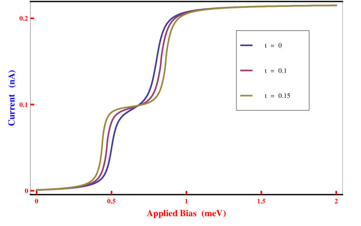
Figure 1: Current as a function of applied bias. The energies of two levels are $\epsilon_{{}_{1}}=0.5meV$, $\epsilon_{{}_{2}}=0.8meV$ . The tunneling rates from the two states are $\Gamma_{ii}=0.04meV$, $\Gamma_{ij}=0meV,$ $where$ $i\neq j.$

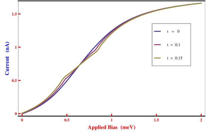
Figure 2: Current as a function of applied bias. The energies of two levels are $\epsilon_{{}_{1}}=0.5meV$, $\epsilon_{{}_{2}}=0.8meV$ . The tunneling rates from the two states are $\Gamma_{ii}=0.4meV$, $\Gamma_{ij}=0meV,$ $where$ $i\neq j.$

These results are also presented in Fig(3) where it is seen that if the lead to the system coupling is small then the energy states of the two dots are sharp and this feature appears as two peaks in the differential conductance. As the lead to the system coupling is increased, the electronic states get broadened. And for sufficiently large tunneling rate (strong lead to system coupling) both the states merge and the peaks in the differential conductance disappear. To observe the effects of inter-dot coupling with in the molecule even as the tunneling rate from the lead to the molecule (lead to molecule coupling) is increased, we show in Fig.(4) that for finite inter-dot coupling, the peaks in the differential conductance persist. The electronic states are broadened due to the coupling of the leads and the molecule but when inter-dot coupling is taken into account, the difference in energy between the levels increases. This compensates the broadening of the levels and allows the two levels to remain distinct. This results in peaks corresponding to the two levels appearing in differential conductance inspite of broadening of the levels, Fig.(4).

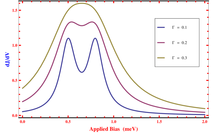
Figure 3: Differential conductance $(dJ/dV)$ as a function of applied bias and tunneling rates. Applied bias and tunneling rates are in the units of meV. The energies of two levels are $\epsilon_{1}=0.5meV$ ,$\epsilon_{2}=0.8meV$ ,$t=0meV$. 

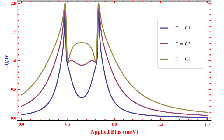
Figure 4: Differential conductance $(dJ/dV)$ as a function of applied bias and tunneling rates. Applied bias and tunneling rates are in the units of meV. The energies of two levels are $\epsilon_{1}=0.5meV$ ,$\epsilon_{2}=0.8meV$ ,$t=0.1meV$. 

At the final stage, we consider the effects of the electron-phonon interaction. These are shown in Figs (5) and (6). We find that in addition to peaks in the differential conductance corresponding to the two levels of the dots there are peaks due to phonons. These phononic peaks (side bands) occur as the electrons can exchange energy with the phonons and contribute to conductance. To focus on the role of inter-dot coupling on phononic peaks, we see that as we increase the (lead to molecule coupling) tunneling rate electronic states are broadened to the extent that phononic side bands are not visible. On further increase in tunneling rate the two electronic states broaden and merge into each other, Fig.(5). If we include inter-dot coupling, not only the electronic states remain distinct but the phononic effects are not lost either. This can be seen in Fig.(6) where peaks appear corresponding to the two electronic states as well as the phononic side band peaks. Even with an increase in tunneling rate from the leads to the molecule, these features persist in the presence of inter-dot coupling.

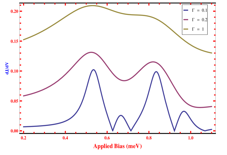
Figure 5: Differential conductance $(dJ/dV)$ as a function of applied bias and tunneling rates. Applied bias and tunneling rates are in the units of meV. The energies of two levels are $\epsilon_{1}=0.5meV$ ,$\epsilon_{2}=0.8meV$ ,$t=0meV$ ,$\ \omega=0.1meV$ ,$\gamma=0.013meV$. 

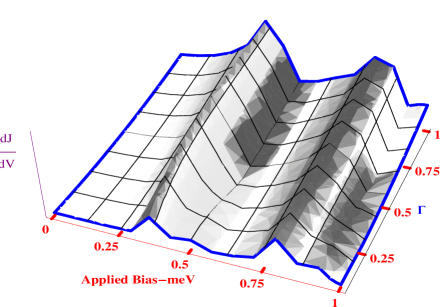
Figure 6: Differential conductance $(dJ/dV)$ as a function of applied bias and tunneling rates. Applied bias and tunneling rates are in the units of meV. The energies of two levels are $\epsilon_{1}=0.5meV$ ,$\epsilon_{2}=0.8meV$ ,$t=0.1meV$ ,$\ \omega=0.1meV$ ,$\gamma=0.013meV$. 

To conclude, in this work we have focused on the role of inter-dot coupling with in the dot molecule on electron transport. We have considered a coupled dot molecule, with inter-dot coupling, attached to two leads including electron-phonon interaction and the coupling of the molecule with an environment allowing dissipation of the phonons. We find that including inter-dot coupling has profound and important role in transport. The step like featues in current voltage characteristics of peaks in differential conductance corresponding to the the dot energy levels is lost in the absence of inter-dot coupling when strong coupling to the leads is considered. Inter-dot coupling allows the two levels to remain distinct with peaks appearing in the differential conductance even when broadening of the levels in the dots occur for strong lead to molecule coupling. Furthermore, phononic side bands that appear in the differential conductance also persist in the presence of finite inter-dot coupling even for strong lead to molecule coupling.

.4.1 Acknowledgements

M. Imran and K. Sabeeh would like to acknowledge the support of the Higher Education Commission (HEC) of Pakistan through project No. 20-1484/R&D/09.

${}^{{}^{\ast}}$imran1gee@gmail.com

^†kashifsabeeh@hotmail.com

References

- (1) A. Aviram, M.A. Ratner, Chem. Phys. Lett. 29, 277 (1974)
- (2) M. A. Reed and J. M. Tour, Sci. Am. 282 , 86.(2000).
- (3) G. Cuniberti, G. Fagas, and K. Richter, Introducing Molecular Electronics, Springer-Verlag, Berlin, (2005) .
- (4) Molecular Nanoelectronics, edited by M. A. Reed and T. LeeAmerican Scientific Publishers, Stevenson Ranch, CA, 2003 .
- (5) D. R. Bowler, J. Phys.: Condens. Matter 16, R721(2004) .
- (6) M.A. Reed, C. Zhou, C.J. Muller, T.P. Burgin, J.M. Tour, Science 278, 252 (1997)
- (7) L. V. Keldysh, Zh. Eksp. Teor. Fiz. 47, 1515 1965 ; H. Huag and A. P. Jauho, Quantum Kinetics in Transport and Optics of Semiconductors, Springer Solid-State Sciences Vol. 123 Springer, New York, (1996).
- (8) E. L¨ortscher, H.B. Weber, H. Riel, Phys. Rev. Lett. 98, 176807 (2007)
- (9) U. Weiss, Quantum Dissipative Systems, Series in Modern Condensed Matter Physics, vol. 10 (World Scientific, 1999)
- (10) H.P. Breuer, F. Petruccione, The theory of open quantum systems (Oxford University Press, Oxford, 2002)
- (11) I.G. Lang, Y.A. Firsov, Sov. Phys. JETP 16, 1301 (1963)
- (12) A.C. Hewson, D.M. Newns, Japan. J. Appl. Phys. Suppl. 2, Pt. 2, 121 (1974)
- (13) G. Mahan, Many-Particle Physics, 2nd edn. (Plenum, New York, 1990)
- (14) Antti-Pekka Jauho, Ned S. Wingreen, and Yigal Meir Phys. Rev. B 50, 5528 (1994)
- (15) Qing-feng Sun and X. C. Xie, Phys.Rev B 75, 155306 (2007).
- (16) A. Hewson and D. Newns, J. Phys. C 13, 4477 (1980)
- (17) Michael Galperin, Abraham Nitzan,and Mark A. Ratner Phys. Rev. B 73, 045314 (2006)
- (18) Z.-Z. Chen, R. Lü, and B.-F. Zhu, Phys. Rev. B 71, 165324(2005).
- (19) M. Di Ventra, S.T. Pantelides, and N. D. Lang, Phys. Rev.Lett. 88, 046801 (2002).
- (20) T. Seideman, J. Phys. Condens. Matter 15, R521 (2003).
- (21) D. A. Ryndyk and J. Keller, Phys. Rev. B 71, 073305 (2005).
- (22) D. A. Ryndyk, M. Hartung, and G. Cuniberti, Phys. Rev. B 73,045420 (2006) .
- (23) S. Datta, W. Tian, S. Hong, R. Reifenberger, J. I. Henderson, andC. P. Kubiak, Phys. Rev. Lett. 79, 2530 (1997) .
- (24) K. Flensberg, Phys. Rev. B 68, 205323,(2003).
- (25) T. Frederiksen, M. Brandbyge, N. Lorente, and A.-P. Jauho, Phys. Rev. Lett. 93, 256601 (2004) .
- (26) M. Galperin, M. A. Ratner, and A. Nitzan, Nano Lett. 4, 1605 (2004) .
- (27) M. Galperin, M. A. Ratner, and A. Nitzan, J. Phys. Chem. 121,11965 (2004) .
- (28) M. Galperin, M. A. Ratner, and A. Nitzan, J. Phys.: Condens.Matter 19, 103201 (2007) .
- (29) L. Kadanoff and G. Baym, Quantum Statistical Mechanics Benjamin,New York, (1962).
- (30) J. Rammer and H. Smith, Rev. Mod. Phys. 58, 323 (1986).
- (31) Y. Meir and N. S. Wingreen, Phys. Rev. Lett. 68, 2512 (1992).
- (32) M. Tahir and A. MacKinnon Phys.Rev B 77, 224305 (2008).
- (33) A.-P. Jauho, J. Phys.: Conf. Ser. 35, 313 (2006).
- (34) W.G. van der Wiel, et.al, Rev. Mod. Phys. 75, 1 (2003).
- (35) S.Tarucha, T. Fujisawa, K. Ono, D.G. Austin, T.H. Oosterkamp, and W.G. van der Wiel, Microelectron. Eng. 47, 101(1999); T. Fujisawa, T.H.Oosterkamp, W.G. van der Wiel, B.W. Broer, R. Aguado, S. Tarucha, and L.P. Kouwenhoven, Science 282, 932(1998); H. Qin, F. Simmel, R.H. Blick, J.P. Kotthaus, W. Wegscheider, and M. Bichler, Phys. Rev. B 63, 035320 (2001); T. Brandes and B. Kramer, Phys. Rev. Lett. 83, 3021 (1999); T. Brandes and N. Lambert, Phys. Rev. B 67, 125323 (2003); T. Fujisawa, D.G. Austing, Y. Tokura, Y. Hirayama, and S. Tarucha, Nature (London) 419, 278 (2002).