Fault-Tolerant Aggregation:
Flow-Updating Meets Mass-Distribution

Abstract

Flow-Updating (FU) is a fault-tolerant technique that has proved to be efficient in practice for the distributed computation of aggregate functions in communication networks where individual processors do not have access to global information. Previous distributed aggregation protocols, based on repeated sharing of input values (or mass) among processors, sometimes called Mass-Distribution (MD) protocols, are not resilient to communication failures (or message loss) because such failures yield a loss of mass.

In this paper, we present a protocol which we call Mass-Distribution with Flow-Updating (MDFU). We obtain MDFU by applying FU techniques to classic MD. We analyze the convergence time of MDFU showing that stochastic message loss produces low overhead. This is the first convergence proof of an FU-based algorithm. We evaluate MDFU experimentally, comparing it with previous MD and FU protocols, and verifying the behavior predicted by the analysis. Finally, given that MDFU incurs a fixed deviation proportional to the message-loss rate, we adjust the accuracy of MDFU heuristically in a new protocol called MDFU with Linear Prediction (MDFU-LP). The evaluation shows that both MDFU and MDFU-LP behave very well in practice, even under high rates of message loss and even changing the input values dynamically.

Keywords. Aggregate computation, Distributed computing, Radio networks, Communication networks.

1 Introduction

The distributed computation of algebraic aggregate functions is particularly challenging in settings where the processing nodes do not have access to global information such as the input size. A good example of such scenario is Sensor Networks [1, 28] where unreliable sensor nodes are deployed at random and the overall number of nodes that actually start up and sense input values may be unknown. Under such conditions, well-known techniques for distributing information throughout the network such as Broadcast [21] or Gossiping [11] cannot be directly applied, and data collection is only practicable if aggregation is performed. Even more challenging is that loss of messages between nodes or even node crashes are likely in such harsh settings. It has been proved [2] that the problem of aggregating values distributedly in networks where processing nodes may join and leave arbitrarily is intractable. Hence, arbitrary adversarial message loss also yields the problem intractable, but a weaker adversary, for instance a stochastic one as in Dynamic Networks [7], is of interest. In this paper, under a stochastic model of message loss, we study communication networks where each node holds an input value and the average of those values  must be obtained by all nodes, none of whom have access to global information of the network, not even the total number of nodes $n$.

A classic distributed technique for aggregation, sometimes called Mass-Distribution (MD) [10], works in rounds. In each round, each node shares a fraction of its current average estimation with other nodes, starting from the input values [19, 3, 5, 6, 33, 32, 27, 29]. Details differ from paper to paper but a common problem is that, in the face of message loss, those protocols either do not converge to a correct output or they require some instantaneous failure detector mechanism that updates the topology information at each node in each round. Recently [18, 17], a heuristic termed Flow-Updating (FU) addressed the problem assuming stochastic message loss [18], and even assuming that input values change and nodes may fail [17]. The idea underlying FU is to keep track of an aggregate function of all communication for each pair of communicating nodes, since the beginning of the protocol, so that a current value at a node can be re-computed from scratch in each round. Empirical evaluation has shown that FU behaves very well in practice [18, 17], but such protocols have eluded analysis until now.

In this paper, we introduce the concept of FU to MD. First, we present a protocol that we call Mass-Distribution with Flow-Updating (MDFU). The main difference with MD is that, instead of computing incrementally, the average is computed from scratch in each round using the initial input value and the accumulated value shared with other nodes so far (which we refer to as either mass shared, or flow passed). The main difference with FU is that if messages are not lost the algorithm is exactly MD, which facilitates the theoretical analysis of the convergence time under failures parameterized by the failure probability (or message-loss rate).

Our results.We first leverage previous work on bounding the mixing time of Markov chains [30] to show that, for any $0<\xi<1$, the convergence time of MDFU under reliable communication is $2\ln(n/\xi)/\Phi(G)^{2}$, where $\Phi(G)$ is the conductance of the underlying graph characterizing the execution of MDFU on the network. Then, we show that, with probability at least $1-1/n$, for a message-loss rate $f<1/\ln(2\Delta e)^{3}$, the multiplicative overhead on the convergence time produced by message loss is less than $1/(1-\sqrt{f\ln(2\Delta e)^{3}})$, and it is constant for $f\leq 1/(e(2\Delta e)^{e})$, where $\Delta$ is the maximum number of neighbors of any node. Also, we show that, with probability at least $1-1/n$, for any $0<\xi<1$, after convergence the expected average estimation at any node is in the interval $[(1-\xi)(1-f)\overline{v},(1+\xi)\overline{v}]$. This is the first convergence proof for an FU-based algorithm.

In MDFU, if some flow is not received, a node computes the current estimation using the last flow received. Thus, in presence of message loss, nodes do not converge to the average and only some parametric bound can be guaranteed as shown. Aiming to improve the accuracy of MDFU, we present a new heuristic protocol that we call MDFU with Linear Prediction (MDFU-LP). The difference with MDFU is that if some flow is not received a node computes the current estimation using an estimation of the flow that should have been received.

We evaluate MDFU and MDFU-LP experimentally and find that the performance of MDFU is comparable to FU and other competing algorithms under reliable communication. In the presence of message loss, the empirical evaluation shows that MDFU behaves as predicted in the analysis converging to the average with a bias proportional to the message-loss rate. This bias is not present in the original FU, which converges to the correct value even under message loss. In a third set of evaluations, we observe that MDFU-LP converges to the correct value even under high message loss rates, with the same speed as under reliable communication. We also test MDFU under changing input values to verify that it tolerates dynamic changes in practice, in contrast to classic MD algorithms, which need to restart the computation each time values are changed.

Roadmap. In Section 2 we formally define the model and the problem, and we give an overview of related work. Section 3 includes the details of MDFU and its analysis, whereas its empirical evaluation is covered in Section 4. In Section 5 we present the details of MDFU-LP and its experimental evaluation. Section 6 evaluates MDFU in a dynamic setting, where input values change over time.

2 Preliminaries

Model. We consider a static connected communication network formed by a set $V$ of $n$ processing nodes. We assume that each node has an identifier (ID). Any pair of nodes $i,j\in V$ such that $i$ may send messages to $j$ without relying on other nodes (one hop) are called neighbors. We assume that the IDs are assigned so that each node is able to distinguish all its neighbors. The set of ordered pairs of neighbors (or, edges) is called $E$. The network is symmetric, meaning that, for any $i,j\in V$, $(i,j)\in E$ if and only if $(j,i)\in E$. The set of neighbors of a given node $i$ is denoted as $N_{i}$ and $|N_{i}|$ is called the degree of $i$. For each pair of nodes $i,j\in V$, the maximum degree between $i,j$ is denoted as $D_{ij}=\max\{|N_{i}|,|N_{j}|\}$. The maximum degree throughout the network is denoted as $\Delta=\max_{i\in V}|N_{i}|$. Each node $i$ knows $N_{i}$ and $D_{ij}$ for each $j\in N_{i}$, but does not know the size of the whole network $n$. The time is slotted in rounds and each round is divided in two phases. In each round, a node is able to send (resp. receive) one message to (resp. from) all its neighbors (communication phase) and to perform local computations (computation phase). However, for each $(i,j)\in E$ and for each communication phase, a message from $i$ to $j$ is lost independently with probability $f$. This is a crucial difference with previous work where, although edge-failures are considered, messages are not lost thanks to the availability of some failure detection mechanism. More details are given in the previous work section. Nodes are assumed to be reliable, i.e. they do not fail.

Problem. Each node $i$ holds an input value $v_{i}$, for $1\leq i\leq n$. The aim is for each node to compute the average $\overline{v}=\sum_{i=1}^{n}v_{i}/n$ without any global knowledge of the network. We focus on the algorithmic cost of such computation, counting only the number of rounds that the computation takes after simultaneous startup of all nodes, leaving aside medium access issues to other layers. This assumption could be removed as in [10].

Previous Work. Previous work on aggregate computations has been particularly prolific for the area of Radio Networks, including both theoretical and experimental work [20, 8, 12, 16, 19, 35, 23, 26, 24, 22, 14, 15, 13]. Many of those and other aggregation techniques exploit global information of the network [10, 22, 23, 12], or are not resilient to message loss [3, 19, 5].

FU is a recent fault-tolerant approach[18, 17] inspired on the concept of flows (from graph theory). Like common MD techniques, it is based on the execution of an iterative averaging process at all nodes, and all estimates eventually converge to the system-wide average. MD protocols exchange “mass”, which lead them to converge to a wrong result in the case of message loss. In contrast, FU does not exchange “mass”. Instead it performs idempotent flow exchanges which provide resilience against message loss. In particular, FU keeps the initial input value at each node unchanged (in a sense, always conserving the global mass), exchanging and updating flows between neighbors for them to produce a new estimate. The estimate is computed at each node from the input values and the contribution of the flows. No theoretical bounds on the performance of the algorithm were provided. Empirical evaluation shows that FU performs better than classic MD algorithms, especially in low-degree networks, and it supports high levels of message loss [18]. Moreover, it self-adapts to dynamic changes (i.e. nodes leaving/arriving and input value change) without any restart mechanism (like other approaches), and tolerates node crashes [17].

MD protocols for average computations in arbitrary networks based on gossiping (exchange values in pairs) were studied in [3, 19]. Results in [3] are presented for all gossip-based algorithms by characterizing them by a matrix that models how the algorithm evolves while sharing values in pairs iteratively. As in our results, the time bounds shown are given as a function of the spectral decomposition of the graph underlying the computation. The work is focused on optimizing distributedly the spectral gap, in order to minimize convergence time. The dynamics of the model are motivated by changes in topology induced by nodes leaving and joining the network. Those changes may be introduced in the probability of establishing communication between any two nodes. However, the delivery of messages has to be reliable to ensure mass conservation. An algorithm called Push-Sum that takes advantage of the broadcast nature of Radio Networks (i.e., it is not restricted to gossip) is included in [19], yielding similar bounds. Chen, Pandurangan, and Hu [5] present an MD algorithm that first builds a forest over the network, where each root collects the information, and then a gossiping algorithm among the roots is used. The authors show a reduction on the energy consumption with respect to the uniform gossip algorithm. On the other hand, the MD algorithm presented in [6] relies on a different randomly chosen local leader in each round to distribute values. The bounds given are also parameterized by the eigen-structure of the underlying graph. This result was extended more recently [4] to networks with a time-varying connection graph, but the protocol requires to update the matrix underlying such graph in each round.

MD protocols have been used also for Distributed Average Consensus [33, 34, 32, 27, 29, 31] within Control Theory, but they do not apply to our model. For example, in [33, 34] the model includes unreliable communication links, but the algorithm requires instantaneous update of the topology information held at each node at the beginning of each round. Others, either rely on similar features [27, 29, 31] or do not consider changes in topology at all [32].

The common problem in all the MD protocols is that they are not resilient to message loss, because it implies a loss of mass. Hence, if messages are lost, they need to restart the computation from scratch. In MDFU, message loss has an impact on convergence time, which we show to be small, but the computation recovers from those losses, yielding the correct value. In fact, it is this characteristic of MDFU and FU in general what makes the technique suitable for dynamic settings in which the input values change with time.

3 MDFU

// initialization

$e_{i}\leftarrow v_{i}$

foreach $j\in N_{i}$ do $F_{in}(j)\leftarrow 0$

$F_{out}(j)\leftarrow e_{i}/\left(2D_{ij}\right)$

foreach round do // communication phase

foreach $j\in N_{i}$ do Send $j$ message $\langle i,F_{out}(j)\rangle$

foreach $\langle j,F\rangle$ received do $F_{in}(j)\leftarrow F$

// computation phase

$e_{i}\leftarrow v_{i}+\sum_{j\in N_{i}}(F_{in}(j)-F_{out}(j))$

foreach $j\in N_{i}$ do $F_{out}(j)\leftarrow F_{out}(j)+e_{i}/\left(2D_{ij}\right)$

Algorithm 1 MDFU. Pseudocode for node $i$. $e_{i}$ is the estimate of node $i$. $F_{in}(j)$ is the cumulative inflow from node $j$. $F_{out}(j)$ is the cumulative outflow to node $j$.

10

10

10

10

10

10

10

10

10

10

As in previous work [19, 6, 3, 10], MDFU is based on repeatedly sharing among neighbors a fraction of the average estimated so far. Unlike in those papers, in MDFU the estimation is computed from scratch in each round, as in FU [18, 17]. For that purpose, each node keeps track of the cumulative value passed to each neighbor (or, cumulative flow) since the protocol started. Together with the original input value, those flows allow each node to recompute the average estimation in each round. Should some flow from node $i$ to node $j$ be lost, $j$ temporarily computes the estimation using the last flow received from $i$. Further details can be found in Algorithm 1.

Recall that the aim is to compute the average $\overline{v}=\sum_{i=1}^{n}v_{i}/n$ of all input values. Let $e_{i}(r)$ be the average estimate of node $i$ in round $r$, and $\varepsilon(r)=\max_{i}\{|e_{i}(r)-\overline{v}|/\overline{v}\}$ be the maximum relative error of the average estimates in round $r$. We want to bound the number of rounds after which the maximum relative error is below some parametric value $\xi$.

In each round, a node shares a fraction of its current estimate with each neighbor. Therefore, the execution of each round can be characterized by a transition matrix, denoted as $\mathbf{P}=(p_{ij})$, $\forall i,j\in V$, such that for any round $r$ where messages are not lost

$$p_{ij}=\left\{\begin{array}[]{ll}1/(2D_{ij})&\textrm{if $i\neq j$ and $(i,j)\in E$,}\\ 1-\sum_{k\in N_{i}}1/(2D_{ik})&\textrm{if $i=j$,}\\ 0&\textrm{$(i,j)\notin E$}\end{array}\right.$$

and $\mathbf{e}(r+1)=\mathbf{e}(r)\mathbf{P}$, where $\mathbf{e}(\cdot)$ is the row vector $(e_{1}(\cdot)e_{2}(\cdot)\dots e_{n}(\cdot))$.

3.1 Convergence Time for $f=0$

Consider first the case when the communication is reliable, that is $f=0$. Then, the above characterization is round independent and, given that $\mathbf{P}$ is stochastic, it can be seen as the transition matrix of a time-homogeneous Markov chain $(X_{r})_{r=1}^{\infty}$ with finite state space $V$. Furthermore, $(X_{r})_{r=1}^{\infty}$ is irreducible, and aperiodic, then it is ergodic and it has a unique stationary distribution. Given that $\mathbf{P}$ is doubly stochastic such stationary distribution is $\pi_{i}=1/n$ for all $i\in V$. Thus, bounding the convergence time of $(X_{r})_{r=1}^{\infty}$ we have a bound for the convergence time of MDFU without message loss. The following notation will be useful. Let $G$ be a weighted undirected graph with set of nodes $V$ and where, for each pair $i,j\in V$, the edge $(i,j)$ has weight $\pi_{i}p_{ij}$. $G$ is called the underlying graph of the Markov chain $(X_{r})_{r=1}^{\infty}$. The following quantity characterizes the likelihood that the chain does not stay in a subset of the state space with small stationary probability. Let the conductance of graph $G$ be

$$\Phi(G)=\min_{\begin{subarray}{c}\emptyset\subset S\subset V\\ \sum_{i\in S}\pi_{i}\leq 1/2\end{subarray}}\frac{\sum_{i,j\in S}p_{ij}\pi_{i}}{\sum_{i\in S}\pi_{i}}.$$

The following theorem shows the convergence time of MDFU with reliable communication parameterized in the conductance of $G$.

Theorem 3.1

For any communication network of $n$ nodes running MDFU, for any $0<\xi<1$, and for $r_{c}=2\ln(n/\xi)/\Phi(G)^{2}$, if $f=0$, it holds that $\varepsilon(r)\leq\xi$ for any round $r\geq r_{c}$, where $\Phi(G)$ is the conductance of the underlying graph characterizing the execution of MDFU on the network.

Proof

We want to find a value of $r_{c}$ such that for all $r\geq r_{c}$ it holds that $\max_{i}\{|e_{i}(r)-\overline{v}|/\overline{v}\}\leq\xi$. Then, we want $\max_{i}\{|e_{i}(r)/\sum_{j\in V}v_{j}-1/n|\}\leq\xi/n$. Given that $e_{i}(r)=\sum_{j\in V}v_{j}(\mathbf{P}^{r})_{ji}$, it is enough to have $\max_{j,i\in V}\{|(\mathbf{P}^{r})_{ji}-1/n|\}\leq\xi/n$. On the other hand, given that $p_{ij}\pi_{i}=p_{ji}\pi_{j}$ for all $i,j\in V$, the Markov chain is time-reversible. Then, as proved in [30], it is $\max_{i,j\in V}|(\mathbf{P}^{r})_{ij}-\pi_{j}|/\pi_{j}\leq\lambda^{r}_{1}/\min_{j\in V}\pi_{j}$, where $\lambda_{1}$ is the second largest eigenvalue of $\mathbf{P}$ (all the eigenvalues of $\mathbf{P}$ are positive because $p_{ii}\geq 1/2$ for all $i\in V$). Given that $\pi_{i}=1/n$ for all $i\in V$, we have $\max_{i,j\in V}|(\mathbf{P}^{r})_{ij}-1/n|\leq\lambda^{r}_{1}$. Thus, from the inequality above, it is enough to have $\lambda^{r}_{1}\leq\xi/n$. As proved also in [30], given that $(X_{r})_{r=1}^{\infty}$ is ergodic and time-reversible, it is $\lambda_{1}\leq 1-\Phi(G)^{2}/2$. Then, it is enough $(1-\Phi(G)^{2}/2)^{r}\leq\xi/n$. Given that $\Phi(G)\leq 1$, using that $1-x\leq e^{-x}$ for $x<1$, the claim follows.

3.2 Convergence Time for $f>0$

Mixing time of a multiple random walk. Recall that we carry out an average computation of $n$ input values where each node $i$ shares a $1/(2D_{ij})$ fraction of its estimate in each round of the computation with each neighboring node $j$. We have characterized each round of the computation with a transition matrix $\mathbf{P}$ so that in each round $r$ the vector of estimates $\mathbf{e}(r)$ is multiplied by $\mathbf{P}$.

The Markov chain defined in Section 3.1 that models the average computation is also a characterization of a random walk, that is, a stochastic process on the set of nodes $V$ where a particle moves around the network randomly. In our case, for each round, instead of choosing the next node where the particle will be located uniformly among neighbors, the matrix of transition probabilities is $\mathbf{P}$. A state of this process (which of course is also Markovian) is a distribution of the location of the particle over the nodes. The measure of this random walk that becomes relevant in our application is the mixing time, that is, the number of rounds before such distribution will be close to uniform. The mixing time of this random walk is the same as the convergence time of the Markov chain $(X_{r})_{r=1}^{\infty}$, setting appropriately for each case the desired maximum deviation with respect to the stationary distribution as follows.

A useful representation of this process in our application is to assume a set $S$ of particles, all of the same value $\nu$, so that at the beginning each node $i$ holds a subset $S_{i}$ of particles such that $|S_{i}|\nu=v_{i}$. In order to analyze the computation along many rounds, we assume that $\nu$ is small enough so that particles are not divided. We define the mixing time of this multiple random walk as the number of rounds before the distribution of all particles is within $\xi/n$ of the uniform, for $0<\xi<1$. Without message loss, it can be seen that the mixing time of the above defined multiple random walk is the same as the convergence time of the Markov chain $(X_{r})_{r=1}^{\infty}$ defined in Section 3.1. We consider now the case where messages may be lost.

The following lemma shows that, for $f<1/\ln(2\Delta e)^{3}$, the multiplicative overhead on the mixing time produced by message loss is less than $1/(1-\sqrt{f\ln(2\Delta e)^{3}})$, and it is constant for $f\leq 1/(e(2\Delta e)^{e})$. The proof uses concentration bounds on the delay that any particle may suffer due to message loss.

Lemma 1

Consider any communication network of $n$ nodes running MDFU, any $0<f\leq 1/\ln(2\Delta e)^{3}$, any $0<\xi<1$, let $r_{c}=2\ln(n/\xi)/\Phi(G)^{2}$, and let

$$q=\left\{\begin{array}[]{ll}1/e&\textrm{ if $f\leq 1/(e(2\Delta e)^{e})$}\\ f\left(\sqrt{4\ln(2\Delta e)^{3}/f-3}-1\right)/2&\textrm{ otherwise.}\end{array}\right.$$

Consider a multiple random walk modeling MDFU as described. With probability at least $1-1/n$, after $r=r_{c}/(1-q)$ rounds it holds that $\max_{x\in S,i\in V}|p_{x}(i)-1/n|\leq\xi/n$, where $p_{x}(i)$ is the probability that particle $x$ is located at node $i$.

Proof

For clarity, we model the network with a directed graph $\{V,E\}$, with $V$ and $E$ as defined in the model. A message loss in the edge $(i,j)\in E$ is modeled with a buffer on the edge $(i,j)$ where a particle is “delayed”. For a computation of $r$ rounds, it is enough to consider at most $n(2\Delta)^{r}$ particles, because initially there are $n$ input values and each value is divided $r$ times by at most $2\Delta$. Consider the random walk of a given particle $x\in S$. For each round, $x$ is delayed with probability $f$. We bound the mixing time by bounding the number of rounds that any particle is delayed as follows.

Assume first that $1/(e(2\Delta e)^{e})<f\leq 1/\ln(2\Delta e)^{3}$. For $r$ rounds, the expected number of rounds when a given particle is delayed is $fr$. Using Chernoff-Hoeffding bounds [25], the probability that a given particle $x$ is delayed more than $qr$ rounds, $f\leq q\leq 1$, is at most $\exp(-fr(q/f-1)^{2}/3)$. Then, the probability that some particle is delayed more than $qr$ rounds is

$$\mathbf{Pr}(\textrm{$\exists x:x$ delayed $>qr$}) \leq n\left(\frac{2\Delta}{\exp((q-f)^{2}/(3f))}\right)^{r}.$$

Assuming that $2\Delta\exp(1-q)\leq\exp((q-f)^{2}/(3f))$, we get that

$$\mathbf{Pr}(\textrm{$\exists x:x$ delayed $>qr$}) \leq n\left(\frac{1}{\exp(1-q)}\right)^{\frac{2\ln(n/\xi)}{(1-q)\Phi(G)^{2}}}$$

$$=n\exp\left(-\frac{2\ln(n/\xi)}{\Phi(G)^{2}}\right),\textrm{given that $\xi\leq 1$ and $\Phi(G)\leq 1$,}$$

$$\leq n\exp(-2\ln n)$$

$$=1/n.$$

Then, it remains to prove

$$2\Delta\exp(1-q) \leq\exp((q-f)^{2}/(3f))$$

$$q^{2}+fq+f^{2}-f\ln(2\Delta e)^{3} \geq 0.$$

Which is true for $q=f\left(\sqrt{4\ln(2\Delta e)^{3}/f-3}-1\right)/2$, which is feasible because, for $f\leq 1/\ln(2\Delta e)^{3}$, such value of $q$ implies $f\leq q\leq 1$ .

Consider now the case $0<f\leq 1/(e(2\Delta e)^{e})$. Again, using Chernoff-Hoeffding bounds, the probability that a given particle $x$ is delayed more than $qr$ rounds, $f\leq q\leq 1$, is at most $\left((fe/q)^{q}/e^{f}\right)^{r}$ Then, the probability that some particle is delayed more than $qr$ rounds is

$$\mathbf{Pr}(\textrm{$\exists x:x$ delayed $>qr$}) \leq n\left(\frac{2\Delta}{e^{f}}\left(\frac{fe}{q}\right)^{q}\right)^{r}.$$

Assuming that $2\Delta(fe/q)^{q}/e^{f}\leq 1/\exp(1-q)$ we get as before,

$$\mathbf{Pr}(\textrm{$\exists x:x$ delayed $>qr$}) \leq 1/n.$$

Then, it remains to prove

$$\frac{2\Delta}{e^{f}}\left(\frac{fe}{q}\right)^{q} \leq\frac{1}{e^{1-q}}$$

$$2\Delta e^{1-f} \leq\left(q/f\right)^{q}$$

$$2\Delta e \leq\left(q/f\right)^{q}.$$

Which is true for $f\leq 1/(e(2\Delta e)^{e})$ and $q=1/e$.

The expected number of particles at each node as a function of $f$. Analyzing a multiple random walk of a set of particles, in Lemma 1 we obtained a bound on the time that any particle takes to converge to a stationary uniform distribution. However, for any probability of message loss $f>0$ and for any round, there is a positive probability that some particles are located in the edge buffers defined in the proof of such lemma. Hence, the fact that each particle is uniformly distributed over nodes does not imply that the expected average held at the nodes has converged, because only particles located at nodes are uniformly distributed. We bound the expected error in this section. The proof of the following lemma is based on computing the overall expected ratio of particles in nodes with respect to delayed particles.

Lemma 2

Consider a multiple random walk modeling MDFU under the conditions of Lemma 1. Then, with probability at least $1-1/n$, for any round $r\geq r_{c}/(1-q)$, the expected number of particles $\mathbf{E}(|S_{i}^{(r)}|)$ in each node $i$ is $(1-\xi)(1-f)|S|/n\leq\mathbf{E}(|S_{i}^{(r)}|)\leq(1+\xi)|S|/n$.

Proof

We consider a multiple random walk of a set of particles $S$ over a directed graph $V,E$, with $V$ and $E$ as defined in the model. A message loss in the edge $(i,j)\in E$ is modeled with a buffer on the edge $(i,j)$ where a particle is “delayed”. The following notation will be useful. For any round $r$, $S_{X}^{(r)}$ is the set of particles held at the set $X$ (node set or edge-buffer set), and $S_{i}^{(r)}$ is the set of particles held at the node $i$. Let $p_{i}=\sum_{j_{\in}N_{i}}1/(2D_{ij})$ for any node $i$. By linearity of expectation, at the end of round $r$, the expected number of particles in all buffer-edges and the expected number of particles in all nodes are

$$\mathbf{E}(|S_{E}^{(r)}|) =\sum_{i\in V}\mathbf{E}(|S_{i}^{(r-1)}|)fp_{i}+f\mathbf{E}(|S_{E}^{(r-1)}|)$$ (1)

$$\mathbf{E}(|S_{V}^{(r)}|) =\sum_{i\in V}\mathbf{E}(|S_{i}^{(r-1)}|)(1-fp_{i})+(1-f)\mathbf{E}(|S_{E}^{(r-1)}|).$$ (2)

Using that $p_{i}\leq 1/2$ in 1 and 2, we have

$$\mathbf{E}(|S_{E}^{(r)}|) \leq(f/2)\mathbf{E}(|S_{V}^{(r-1)}|)+f\mathbf{E}(|S_{E}^{(r-1)}|)$$

$$\mathbf{E}(|S_{V}^{(r)}|) \geq(1-f/2)\mathbf{E}(|S_{V}^{(r-1)}|)+(1-f)\mathbf{E}(|S_{E}^{(r-1)}|).$$

Then,

$$\frac{\mathbf{E}(|S_{E}^{(r)}|)}{\mathbf{E}(|S_{V}^{(r)}|)} \leq\frac{(f/2)\mathbf{E}(|S_{V}^{(r-1)}|)+f\mathbf{E}(|S_{E}^{(r-1)}|)}{(1-f/2)\mathbf{E}(|S_{V}^{(r-1)}|)+(1-f)\mathbf{E}(|S_{E}^{(r-1)}|)}$$

$$\leq\frac{f}{1-f},\textrm{ because }\frac{1-f/2}{1-f}\geq\frac{1}{2}.$$

Then, given that $\mathbf{E}(|S_{V}^{(r)}|)+\mathbf{E}(|S_{E}^{(r)}|)=|S|$, we have $\mathbf{E}(|S_{V}^{(r)}|)\geq(1-f)|S|$. As proved in Lemma 1, with probability at least $1-1/n$, for any round $r\geq r_{c}/(1-q)$, $\max_{x\in S,i\in V}|p_{x}(i)-1/n|\leq\xi/n$, where $p_{x}(i)$ is the probability that particle $x$ is located at node $i$ and $q$ as defined in such lemma. Then, for any node $i\in V$, it is $(1-\xi)(1-f)|S|/n\leq\mathbf{E}(|S_{i}^{(r)}|)\leq(1+\xi)|S|/n$ and the claim follows.

Based on the previous lemmata, the following theorem shows the convergence time of MDFU.

Theorem 3.2

Consider any communication network of $n$ nodes running MDFU. For any $0<f\leq 1/\ln(2\Delta e)^{3}$, let $q=1/e$ if $f\leq 1/(e(2\Delta e)^{e})$, or $q=f\left(\sqrt{4\ln(2\Delta e)^{3}/f-3}-1\right)/2$ otherwise, and let $r_{c}=2\ln(n/\xi)/\Phi(G)^{2}$. Then, with probability at least $1-1/n$, for any $0<\xi<1$ and any round $r\geq r_{c}/(1-q)$, the expected average estimation at any node $i\in V$ is $(1-\xi)(1-f)\overline{v}\leq\mathbf{E}(e_{i}^{(r)})\leq(1+\xi)\overline{v}$, where $\Phi(G)$ is the conductance of the underlying graph characterizing the execution of MDFU on the network.

Proof

From Lemmas 1 and 2, we know that, under the conditions of this theorem, for any round $r\geq r_{c}/(1-q)$ and any node $i\in V$, with probability at least $1-1/n$ the expected number of particles (of the multiple random walk modeling MDFU) is $(1-\xi)(1-f)|S|/n\leq\mathbf{E}(|S_{i}^{(r)}|)\leq(1+\xi)|S|/n$. Then, multiplying by the value of each particle the claim follows.

4 Empirical Evaluation of MDFU

We evalutated MDFU in a synchronous network simulator, using an Erdős–Rényi[9] network with 1000 nodes and 5000 links (giving an average degree of 10). The input values were chosen as when performing node counting [16]; i.e., all values being 0 except a random node with value 1; this scenario is more demanding, leading to slower convergence, than uniformly random input values. The evaluation aimed at: 1) comparing its convergence speed under no loss with competing algorithms; 2) evaluating its behavior under message loss; 3) checking its ability to perform continuous estimation over time-varying input values.

4.1 Convergence Speed Against Related Algorithms Under no Faults

To evaluate wether MDFU is a practical algorithm in terms of convergence speed, we compared it against three other algorithms: the original Flow-Updating [18, 17](FU), Distributed Random Grouping [6] (DRG), and Push-Synopses [19]. Figure 1 shows the coefficient of variation of the root mean square error as a function of the number of rounds (averaging 30 runs), with CV(RMSE) = $\sqrt{\sum_{i\in V}(e_{i}-\overline{v})^{2}/n}/\overline{v}$.

It can be seen that MDFU is competitive, providing approximate estimates slightly faster than FU and DRG and giving reasonably accurate results roughly in line with them. It loses to them for very high precision estimation and to Push-Synopses for all precisions (but both DRG and Push-Synopses are not fault-tolerant).

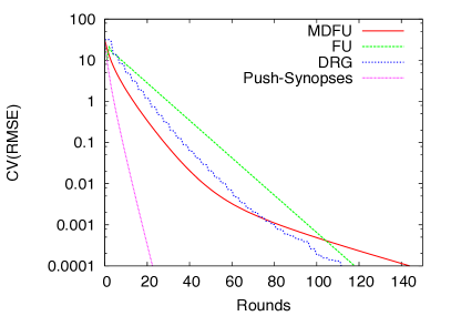
Figure 1: CV(RMSE) over rounds in a 1000 node 5000 link Erdos-Renyi network.

4.2 Fault Tolerance: Resilience to Message Loss

To evaluate the resilience of MDFU to message loss, we performed simulations using different rates of message loss (0, 1%, 5%, 10%), where each individual message may fail to reach the destination with these given probabilities. We measured the effect of message loss on both the CV(RMSE) and also on the maximum relative error. As can be seen in Figure 2, as long as there is some message loss, they do not tend to zero anymore, but converge to a value that is a function of the message loss rate.

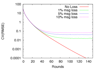
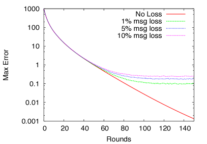
Figure 2: Coefficient of variation of the RMSE and maximum relative error for MDFU in a 1000 node 5000 link Erdos-Renyi network.

We also measured the behavior of the average of the estimates over the whole network, and observed that there is a deviation from the correct value ($\overline{v}$, the average of the input values) towards lower values. Figure 3 shows the relative deviation from the correct value over time, for different message loss rates. It can be seen that this bias is roughly proportional to the message loss rate (for these small message loss rates).

Relating these results with the theoretical analysis of MDFU, we can see that this bias should not come as a surprise. From Theorem 3.2, the expected value of the estimation converges to a band between $(1-f)\overline{v}$ and $\overline{v}$. The relative deviation of the lower boundary is thus proportinal to the message loss rate. Figure 3 also shows this boundary for the different message loss rates.

This kind of bias was not present in the original FU, in which the average of the estimates tends to the correct value. In MDFU the message loss rate limits the precision that can be achieved, but it does not impact convergence, contrary to classic mass distribution algorithms where, given message loss, the more rounds pass, the more mass is lost and the more the estimates deviate from the correct value, failing to converge.

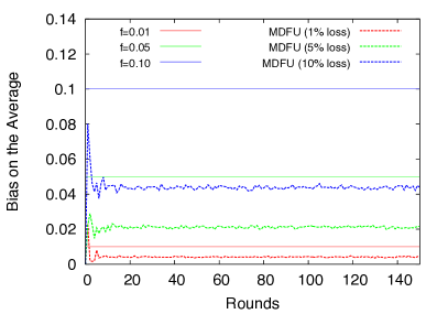
Figure 3: Bias on the average estimation over rounds in a 1000 node 5000 link Erdos-Renyi network.

5 MDFU with Linear Prediction

The explanation for the behavior of MDFU under message loss lies in that only the estimate converges, but flows keep steadily increasing over time. This can be seen in the formula: $F_{out}(j)\leftarrow F_{out}(j)+e_{i}/\left(2D_{ij}\right)$ where the flow sent to some neighbor increases at each round by a value depending on the estimate and their mutual degrees. What happens is that during convergence, the extra flow that each of two nodes send over a link tend to the same value, and the extra outgoing flow cancels out the extra incoming flow. We can say that it is the velocity (rate of increase) of flows over a link that converge (to some different value for each link).

This means that, even if the estimate had already converged to the correct value, given a message loss, the extra flow that should have been received is not added to the estimate, implying a discrete deviation from the correct value. This discrete deviation does not converge to zero; thus, we have a bias towards lower values and the relative estimation error is prevented from converging to zero given some message loss rate.

Here we improve MDFU by exploring velocity convergence. We keep, for each link, the velocity (rate of increase) of the flow received. If a message is lost, we predict what would have been the flow received, given the stored flow, the velocity and the rounds passed since the last message received over that link, i.e., we perform a linear prediction of incoming flow. When a message is received we update the flow and recalculate the velocity. This algorithm is presented in Algorithm 2.

// initialization

$e_{i}\leftarrow v_{i}$

foreach $j\in N_{i}$ do $F_{in}(j)\leftarrow 0$

$F_{out}(j)\leftarrow e_{i}/\left(2D_{ij}\right)$

$V(j)\leftarrow 0$

$R(j)\leftarrow 1$

foreach round do // communication phase

foreach $j\in N_{i}$ do Send $j$ message $\langle i,F_{out}(j)\rangle$

// computation phase

foreach $\langle j,F\rangle$ received do $V(j)\leftarrow(F-F_{in}(j))/R(j)$

$R(j)\leftarrow 0$

$F_{in}(j)\leftarrow F$

$e_{i}\leftarrow v_{i}+\sum_{j\in N_{i}}(F_{in}(j)+V(j)\times R(j)-F_{out}(j))$

foreach $j\in N_{i}$ do $F_{out}(j)\leftarrow F_{out}(j)+e_{i}/\left(2D_{ij}\right)$

$R(j)\leftarrow R(j)+1$

Algorithm 2 MDFU-LP. Pseudocode for node $i$. $e_{i}$ is the estimate of node $i$. $F_{in}(j)$ is the cumulative inflow from node $j$. $F_{out}(j)$ is the cumulative outflow to node $j$. $V(j)$ is the velocity of incoming flow from node $j$. $R(j)$ is the number of rounds since the last message received from node $j$.

15

15

15

15

15

15

15

15

15

15

15

15

15

15

15

Under no message loss MDFU-LP is the same as MDFU and the theoretical results on convergence speed also apply to MDFU-LP. Under message loss the velocities converge over time and the prediction will be increasingly more accurate. Therefore, message loss should not cause discrete deviations in the estimate, allowing the estimation error to converge to zero.

We have evaluated MDFU-LP for the same network as before, but now with a wide range of message loss rates. We have observed that the behavior under message loss rates below 50% is almost indistinguishable from the behavior under no message loss. Figure 4 shows the CVRMSE and maximum relative error for 0%, 60%, 70%, and 80% message loss rates. It can be seen that even for 60% loss rate, after 60 rounds we have basically the same estimation errors as under no message loss.

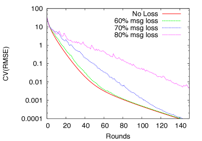
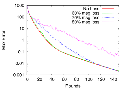
Figure 4: Coefficient of variation of the RMSE and maximum relative error for MDFU-LP in a 1000 node 5000 link Erdos-Renyi network.

6 Continuous Estimation Over Time-Varying Input Values

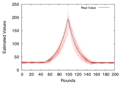
Figure 5: Estimated value over rounds in a 1000 node 5000 link Erdos-Renyi network, with changes of the initial input value at 50% of the nodes.

Up to thus point we have considered that the input values $v_{i}$ are fixed throughout the computation. In most practical situations this will not be the case and input values will change along time. The common approach in MD algorithms is to periodically reset the algorithm and start a new run that freezes the new input values and aggregates the new average. Naturally, resets are inefficient and mechanisms that can adapt the ongoing computation have the potential to adjust the estimates in a much shorter number of rounds.

Without any further modifications, MDFU (and MDFU-LP) share with FU the capability of adapting to input value changes, since $v_{i}$ is considered in the computation of the local estimate $e_{i}$, and this regulates how much the outgoing flows are to be incremented. If $v_{i}$ decreases, $e_{i}$ decreases in the same proportion and node $i$ will share less through its flows to the neighbours. The converse occurring when $v_{i}$ increases. The overall effect is convergence to the new average, even if multiple nodes are having changes in their input values.

In Figure 5 we show an example of how MDFU handles input value changes. In this setting, starting at round 50 and during 50 rounds, we increase by 5% in each round the input value in 500 nodes (a random half of the 1000 nodes). In the following 50 rounds, the same 500 nodes will have its value decreased by 5% per round. Initial input values are chosen uniformly at random (from 25 to 35) and the run is made with message loss at 10%. In Figure 5 one can observe that individual estimates closely follow the global average, with only a slight lag of some rounds.

Notice that the lag could never be zero, since we are updating the new global average (black line) instantaneously and even the fastest theoretical algorithm would need information that takes diameter rounds to acquire.

References

- [1] I. F. Akyildiz, W. Su, Y. Sankarasubramaniam, and E. Cyirci. Wireless sensor networks: A survey. Computer Networks, 38(4):393–422, 2002.
- [2] M. Bawa, H. Garcia-Molina, A. Gionis, and R. Motwani. Estimating aggregates on a peer-to-peer network. Technical report, Stanford University, Database group, 2003.
- [3] Stephen Boyd, Arpita Ghosh, Balaji Prabhakar, and Devavrat Shah. Randomized gossip algorithms. IEEE/ACM Transactions on Networking, 14(SI):2508–2530, 2006.
- [4] Jen-Yeu Chen and Jianghai Hu. Analysis of distributed random grouping for aggregate computation on wireless sensor networks with randomly changing graphs. IEEE Trans. Parallel Distr. Syst., 19(8):1136–1149, 2008.
- [5] Jen-Yeu Chen, Gopal Pandurangan, and Jianghai Hu. Brief announcement: locality-based aggregate computation in wireless sensor networks. In PODC ’09: Proceedings of the 28th ACM symposium on Principles of distributed computing, pages 298–299, New York, NY, USA, 2009. ACM.
- [6] Jen-Yeu Chen, Gopal Pandurangan, and Dongyan Xu. Robust computation of aggregates in wireless sensor networks: distributed randomized algorithms and analysis. IEEE Trans. Parallel Distr. Syst., 17(9):987–1000, 2006.
- [7] A.E.F. Clementi, F. Pasquale, A. Monti, and R. Silvestri. Communication in dynamic radio networks. In Proc. 26th Ann. ACM Symp. on Principles of Distributed Computing, pages 205–214, 2007.
- [8] A. G. Dimakis, A.D. Sarwate, and M.J. Wainwright. Geographic gossip : Efficient averaging for sensor networks. IEEE Transactions on Signal Processing, 56(3):1205–1216, 2008.
- [9] P. Erdos and A. Renyi. On random graphs–i. Publicationes Matematicae, 6:290–297, 1959.
- [10] A. Fernández Anta, M. A. Mosteiro, and C. Thraves. An early-stopping protocol for computing aggregate functions in sensor networks. In Proc. of the IEEE 15th Pacific Rim International Symposium on Dependable Computing, pages 357–364, 2009.
- [11] Leszek Gasieniec. Randomized gossiping in radio networks. In Ming-Yang Kao, editor, Encyclopedia of Algorithms. Springer, 2008.
- [12] Indranil Gupta, Robbert van Renesse, and Kenneth P. Birman. Scalable fault-tolerant aggregation in large process groups. In DSN, pages 433–442. IEEE Computer Society, 2001.
- [13] John S. Heidemann, Fabio Silva, Chalermek Intanagonwiwat, Ramesh Govindan, Deborah Estrin, and Deepak Ganesan. Building efficient wireless sensor networks with low-level naming. In SOSP, pages 146–159, 2001.
- [14] C. Intanagonwiwat, R. Govindan, D. Estrin, J. Heidemann, and F. Silva. Directed diffusion for wireless sensor networking. IEEE/ACM Transactions on Networking, 11(1):2–16, 2003.
- [15] Chalermek Intanagonwiwat, Deborah Estrin, Ramesh Govindan, and John S. Heidemann. Impact of network density on data aggregation in wireless sensor networks. In ICDCS, pages 457–458, 2002.
- [16] Márk Jelasity, Alberto Montresor, and Ozalp Babaoglu. Gossip-based aggregation in large dynamic networks. ACM Transactions on Computer Systems, 23(3):219–252, 2005.
- [17] P. Jesus, C. Baquero, and P.S. Almeida. Fault-tolerant aggregation for dynamic networks. In Proc. of the 29th IEEE Symposium on Reliable Distributed Systems, pages 37–43, 2010.
- [18] Paulo Jesus, Carlos Baquero, and Paulo Almeida. Fault-tolerant aggregation by flow updating. In Proc. of the 9th IFIP WG 6.1 International Conference Distributed Applications and Interoperable Systems, volume 5523 of Lecture Notes in Computer Science, pages 73–86. Springer, 2009.
- [19] D. Kempe, A. Dobra, and J. Gehrke. Gossip-based computation of aggregate information. In Proc. of the 44th IEEE Ann. Symp. on Foundations of Computer Science, pages 482–491, 2003.
- [20] G. Kollios, J. W. Byers, J. Considine, M. Hadjieleftheriou, and F. Li. Robust aggregation in sensor networks. IEEE Data Engineering Bulletin, 28(1):26–32, 2005.
- [21] D. R. Kowalski and A. Pelc. Time complexity of radio broadcasting: adaptiveness vs. obliviousness and randomization vs. determinism. Theoretical Computer Science, 333:355–371, 2005.
- [22] Bhaskar Krishnamachari, Deborah Estrin, and Stephen B. Wicker. The impact of data aggregation in wireless sensor networks. In ICDCS Workshops, pages 575–578. IEEE Computer Society, 2002.
- [23] Samuel Madden, Michael J. Franklin, Joseph M. Hellerstein, and Wei Hong. Tag: a tiny aggregation service for ad-hoc sensor networks. In Proc. of the 5th Symp. on Operating Systems Design and Implementation, pages 131–146, 2002.
- [24] Samuel Madden, Robert Szewczyk, Michael J. Franklin, and David Culler. Supporting aggregate queries over ad-hoc wireless sensor networks. In Proceedings of the Fourth IEEE Workshop on Mobile Computing Systems and Applications, page 49, 2002.
- [25] M. Mitzenmacher and E. Upfal. Probability and Computing: Randomized Algorithms and Probabilistic Analysis. Cambridge University Press, 2005.
- [26] Suman Nath, Phillip B. Gibbons, Srinivasan Seshan, and Zachary R. Anderson. Synopsis diffusion for robust aggregation in sensor networks. In Proceedings of the 2nd international conference on Embedded networked sensor systems, pages 250–262, 2004.
- [27] Reza Olfati-Saber and Richard M. Murray. Consensus problems in networks of agents with switching topology and time-delays. Transactions on Automatic Control, 49(9):1520–1533, 2004.
- [28] P. Rentala, R. Musumuri, U. Saxena, and S. Gandham. Survey on sensor networks. http://citeseer.nj.nec.com/479874.html.
- [29] Dzulkifli S. Scherber and Haralabos C. Papadopoulos. Locally constructed algorithms for distributed computations in ad-hoc networks. In Proceedings of the 3rd International Symposium on Information Processing in Sensor Networks, pages 11–19, 2004.
- [30] Alistair Sinclair and Mark Jerrum. Approximate counting, uniform generation and rapidly mixing markov chains. Information and Computation, 82(1):93–133, 1989.
- [31] D Spanos, R Olfati-Saber, and R Murray. Dynamic consensus on mobile networks. In 16th IFAC World Congress, 2005.
- [32] Lin Xiao and Stephen Boyd. Fast linear iterations for distributed average. Systems and Control Letters, 53:65–78, 2004.
- [33] Lin Xiao, Stephen Boyd, and Sanjay Lall. A scheme for robust distributed sensor fusion based on average consensus. In Proceedings of the 4th International Symposium on Information Processing in Sensor Networks, pages 63–70, 2005.
- [34] Lin Xiao, Stephen Boyd, and Sanjay Lall. A Space-Time Diffusion Scheme for Peer-to-Peer Least-Squares Estimation. In Proceedings of the 5th International Conference on Information Processing in Sensor Networks, pages 168–176, 2006.
- [35] Jerry Zhao, Ramesh Govindan, and Deborah Estrin. Computing aggregates for monitoring wireless sensor networks. In Proc. of the 1st IEEE Intl. Workshop on Sensor Network Protocols and Applications, pages 139–148, 2003.