High dimensional Bayesian inference for Gaussian directed acyclic graph models

Abstract

In this paper, we consider Gaussian models Markov with respect to an arbitrary DAG. We first construct a family of conjugate priors for the Cholesky parametrization of the covariance matrix of such models. This family has as many shape parameters as the DAG has vertices, and naturally extends the work of Geiger and Heckerman [8]. From these distributions, we derive prior distributions for the covariance and precision parameters of the Gaussian DAG Markov models. Our works thus extends the work of Dawid and Lauritzen [5] and Letac and Massam [16] for Gaussian models Markov with respect to a decomposable graph to arbitrary DAGs. For this reason, we call our distributions DAG-Wishart distributions. An advantage of these distributions is that they possess strong hyper Markov properties and thus allow for explicit estimation of the covariance and precision parameters, regardless of the dimension of the problem. They also allow us to develop methodology for model selection and covariance estimation in the space of DAG-Markov models. We demonstrate via several numerical examples that the proposed method scales well to high-dimensions.

1 Introduction

The priors on the parameter of a normal distribution Markov with respect to a DAG now have a long history which starts with [8]. Traditionally these distributions have been derived from some types of (inverse) Wishart distributions and for this reason, we shall call them the DAG-Wishart priors. The different steps in this history are marked by the introduction of more and more flexibility in the shape of the prior. In [8], the prior is derived from the Wishart distribution which has only one shape parameter. Dawid and Lauritzen [5] introduced the hyper inverse Wishart which is the equivalent of the inverse Wishart but for the incomplete covariance matrix which corresponds to the free parameters of a Gaussian distribution Markov with respect to a decomposable graph. Although this is not emphasized in [5], the hyper inverse Wishart is actually equivalent to the DAG-Wishart defined in [8] but for the restricted class of so-called perfect DAGs, those that are Markov equivalent to decomposable graphs. The hyper inverse Wishart still has only one shape parameter. For decomposable graphs, in [16], Letac and Massam introduce a generalization of the hyper inverse Wishart, denoted the $\mathrm{IW}_{\mathrm{P}_{\mathcal{G}}}$ which has $k+1$ multi-shape parameters where $k$ is the number of cliques. This distribution thus offers greater flexibility than the hyper inverse Wishart. We will see that, for the particular case of perfect DAGs, the $\mathrm{IW}_{\mathrm{P}_{\mathcal{G}}}$ is identical to the DAG-Wishart we introduce in this paper.

Indeed, in this paper, we introduce a DAG-Wishart that is similar to the $\mathrm{IW}_{\mathrm{P}_{\mathcal{G}}}$ but introduces yet more flexibility in the choice of multi-shape parameters and is valid for all DAGs and not just the restricted class of perfect DAGs. The hyper inverse Wishart and the $\mathrm{IW}_{\mathrm{P}_{\mathcal{G}}}$ Wishart were derived from the Wishart. In this paper, we proceed in the other direction, we start by defining the multi-shape parameter DAG-Wishart on a convenient space, with one shape parameter for each vertex, and then fold it back into a Wishart-type distribution for the incomplete covariance matrix corresponding to the parametrization of the Gaussian distribution Markov with respect to the DAG. An advantage of the DAG-Wishart distributions proposed in this paper is that, when we use them as priors, high dimensional posterior analysis is readily amenable mainly because these distributions possess hyper Markov properties, which in turn result in closed form solutions for their posterior moments.

The main difficulty in achieving this goal is that when a DAG is no longer perfect defining distributions on the space of covariance or precision matrices is, in a sense, an ill-posed problem, as these spaces are curved manifolds, and thus no distribution defined on them has density with respect to the Lebesgue measure. Consequently, tools for posterior inference on these spaces are not immediately available. For this reason, we need to identify these two spaces with other spaces that yield natural isomorphisms. The new spaces we define here are projections of covariance and precision matrices onto Euclidean space. These are termed the space of incomplete covariance and precision matrices and correspond, respectively, to functionally independent elements of covariance and precision matrix of Gaussian DAG models. Given an incomplete matrix in the space defined by a given DAG, we rely on results and algorithms for completion given in [2] to obtain the corresponding unique covariance and precision matrices of the corresponding Gaussian DAG model. Therefore, with our approach we develop a unified framework for Gaussian DAG models that naturally extends to general DAGs the recent methodological contributions by Letac and Massam [16] and others [18] valid only for decomposable Gaussian graphical models, i.e. perfect DAGs. We also use the DAG-Wishart approach to develop a Bayesian methodology for model selection and covariance estimation that can scale better than any other Bayesian methods that we are aware of.

The remainder of the paper is structured as follows. Section 2 gives a short overview of the basic notation and definitions used in the context of Gaussian DAG models, and formally introduces the Cholesky, precision and covariance parametrizations of Gaussian DAG models. Section 3 introduces the class of generalized Wishart distributions for Gaussian DAG models on the Cholesky space $\Theta_{\mathcal{D}}$ (which we shall name the DAG-Wishart on $\Theta_{\mathcal{D}}$). In Sections 4 and 5 we develop the DAG-Wishart priors on the spaces corresponding to, respectively, the precision and covariance parameterization of DAG models. This entails defining the spaces of incomplete precision and covariance matrices, deriving the densities of the DAG-Wishart distributions on these spaces and formalizing their hyper Markov properties and closed form expressions for posterior quantities. In Section 6, we illustrate the applicability of our DAG-Wishart prior both for covariance/precision matrix estimation and for model selection in the space of models Markov with respect to DAGs with a given order of the vertices. We compare the performance of our method using the DAG-Wishart as a prior with the Lasso-DAG method as in [21]. We show that our approach gives good model selection results and scales well to higher dimensions. Section 7 concludes by briefly summarizing the results in the paper. The Supplemental sections give further details on various results.

2 Preliminaries

A brief summary of graph theory, associated Markov and other properties required for analyzing DAG models is given in Supplemental section A.

2.1 Gaussian DAG models

Let $V$ be a set with $p$ elements. For any $a,b\subseteq V$ let $\mathbb{R}^{a\times b}$ denote the real linear space of functions $A\equiv\left((i,j)\mapsto A_{ij}\right):a\times b\rightarrow\mathbb{R}$. Each element of $\mathbb{R}^{a\times b}$ is called an $|a|\times|b|$ matrix. In particular, we define the space of symmetric matrices ${S}_{a}(\mathbb{R})=\left\{A\in\mathbb{R}^{a\times a}:A_{ij}=A_{ji}~{},\;\text{for every $i,j\in a$}\right\}$, and the set of positive definite matrices $\mathrm{PD}_{a}(\mathbb{R})=\left\{A\in{S}_{a}(\mathbb{R}):~{}x^{\top}Ax>0,\;\text{for every}\>\;x\in\mathbb{R}^{a}\setminus\left\{0\right\}\right\}$. Now let $\Sigma\succ 0$ denote $\Sigma\in\mathrm{PD}_{p}(\mathbb{R})$. For a partition $a,b$ of $V$, consider the corresponding block partitioning of $\Sigma$ as follows.

$$\Sigma=\left(\begin{matrix}\Sigma_{a}&\Sigma_{ab}\\ \Sigma_{ba}&\Sigma_{b}\end{matrix}\right),$$

where $\Sigma_{aa}=(\Sigma_{ij})_{i,j\in a}\in\mathrm{PD}_{a}(\mathbb{R})$, $\Sigma_{bb}=(\Sigma_{ij})_{i,j\in b}\in\mathrm{PD}_{b}(\mathbb{R})$, $\Sigma_{ab}=(\Sigma_{ij})_{i\in a,j\in b}\in\mathbb{R}^{a\times b}$ and $\Sigma_{ba}=\Sigma_{ab}^{\top}$. The Schur complement of the sub-matrix $\Sigma_{aa}$ is defined as $\Sigma_{bb|a}=\Sigma_{bb}-\Sigma_{ba}(\Sigma_{aa})^{-1}\Sigma_{ab}$.

Remark 2.1.

Throughout this paper, we shall in general suppress the notation for a principal submatrix $\Sigma_{aa}$ and refer to it as $\Sigma_{a}$. We shall also use the convention $\Sigma_{a}^{-1}$ for $(\Sigma_{aa})^{-1}$ and $\Sigma^{a}$ for $(\Sigma^{-1})_{aa}$.

In this paper we focus on multivariate Gaussian distributions which obey the directed Markov property with respect to a DAG $\mathcal{D}$. From now on and unless otherwise stated, we shall always assume without loss of generality that $\mathcal{D}=(V,E)$ is a DAG given in a parent ordering, i.e., the vertices are labeled $1,2,\ldots,p$, and $i\rightarrow j$ implies that $i>j$. A Gaussian DAG model (or Gaussian Bayesian network) over $\mathcal{D}$, denoted by $\mathscr{N}(\mathcal{D})$, is the statistical model that consists of all multivariate Gaussian distributions $\rm{N}_{p}(\mu,\Sigma)$ obeying the ordered directed Markov property with respect to $\mathcal{D}$. Therefore, $\mathbf{x}\sim\rm{N}_{p}(\mu,\Sigma)\in\mathscr{N}(\mathcal{D})\implies x_{i}\perp\!\!\!\perp\mathbf{x}_{\left\{i+1,\ldots,p\right\}\setminus\mathrm{pa}(i)}|\mathbf{x}_{\mathrm{pa}(i)}$ for each $i$.

Remark 2.2.

Note that $\rm{N}_{p}(\mu,\Sigma)\in\mathscr{N}(\mathcal{D})$ if and only if $\rm{N}_{p}(0,\Sigma)\in\mathscr{N}(\mathcal{D})$. Therefore, without loss of generality, we shall only consider centered Gaussian distributions

$$\left\{\rm{N}_{p}(0,\Sigma):~{}\Sigma\in\mathrm{PD}_{\mathcal{D}}\right\}\subseteq\mathscr{N}(\mathcal{D}).$$

For convenience, with a slight abuse of notation, we shall still denote

$$\mathscr{N}(\mathcal{D})=\left\{\rm{N}_{p}(0,\Sigma):~{}\Sigma\in\mathrm{PD}_{\mathcal{D}}\right\}.$$

The Gaussian distributions in $\mathscr{N}(\mathcal{D})$ are naturally parametrized by the elements of

$$\mathrm{PD}_{\mathcal{D}}=\left\{\Sigma\succ 0:\>\rm{N}_{p}(0,\Sigma)\in\mathscr{N}(\mathcal{D})\right\}\text{ or }\>\mathrm{P}_{\mathcal{D}}=\left\{\Sigma^{-1}\succ 0:\>\rm{N}_{p}(0,\Sigma)\in\mathscr{N}(\mathcal{D})\right\}.$$

These sets are referred to as the space of covariance matrices and the space of precision matrices. A precision matrix in $\mathrm{P}_{\mathcal{D}}$ is usually denoted by $\Omega$. Similarly, for an undirected graph $\mathcal{G}=(V,\mathscr{E})$ we define $\mathscr{N}(\mathcal{G})$ as the set of multivariate Gaussian distributions obeying the (undirected) Markov property with respect to $\mathcal{G}$. In this model the corresponding parameter spaces are the space of covariance matrices $\mathrm{PD}_{\mathcal{G}}=\left\{\Sigma:\rm{N}_{p}(0,\Sigma)\in\mathscr{N}(\mathcal{G})\right\}$ and the space of precision matrices $\mathrm{P}_{\mathcal{G}}=\left\{\Omega:\Omega^{-1}\in\mathrm{PD}_{\mathcal{G}}\right\}$. Note that, for us, $\mathrm{PD}_{\mathcal{D}}$ and $\mathrm{P}_{\mathcal{D}}$ are parameter spaces of primary interest as they arise naturally in the parameterization of Gaussian densities. However, in order to develop multi-shape parameters Wishart priors on these spaces, which is the main purpose of this paper,we begin with the more natural and more convenient Cholesky type parameterization of $\mathscr{N}(\mathcal{D})$ that we discuss in the next subsection.

2.2 Cholesky parametrizations of Gaussian DAG models

Consider a Gaussian DAG distribution $\rm{N}_{p}(0,\Sigma)\in\mathscr{N}(\mathcal{D})$. It is a well-known fact that the structure of the DAG $\mathcal{D}$ is reflected in the Cholesky decomposition of the precision matrix $\Sigma^{-1}$. A precise explanation is as follows. Let $\mathcal{L}_{\mathcal{D}}$ denote the set of lower triangular matrices with unit diagonals and $L_{ij}=0$ if $i\notin pa(j)$, and let $\mathcal{D}_{+}^{p}$ denote the set of strictly positive diagonal matrices in $\mathbb{R}^{p\times p}$. Then $\Sigma^{-1}\in\mathrm{P}_{\mathcal{D}}$ if and only if there exist $L\in\mathcal{L}_{\mathcal{D}}$ and $D\in\mathcal{D}_{+}^{p}$ such that $\Sigma^{-1}=LD^{-1}L^{\top}$. The latter decomposition of $\Omega=\Sigma^{-1}$ is called the modified Cholesky decomposition of $\Omega$. We call $\Theta_{\mathcal{D}}=\mathcal{D}_{+}^{p}\times\mathcal{L}_{\mathcal{D}}$ the Cholesky space of $\mathcal{D}$, the pair $(D,L)\in\Theta_{\mathcal{D}}$ a Cholesky parameter, and $\left\{\mathrm{N}_{p}(0,\left(L^{\top}\right)^{-1}DL):\>(D,L)\in\Theta_{\mathcal{D}}\right\}\equiv\mathscr{N}(\mathcal{D})$ as the Cholesky parametrization of $\mathscr{N}(\mathcal{D})$.

We can also obtain a variant of this parameterization, in vector form, from the recursive factorization property of the Gaussian densities in $\mathscr{N}(\mathcal{D})$ (see Supplemental section A subsection 1.3 for details). First, let us recall the following notation from [1].
Notation. For each $i\in V$ let

$$\begin{array}[]{lcl}\prec i\succ=pa(i)&\quad[i\succ=\left\{i\right\}\times pa(i)&\quad\prec i]=pa(i)\times\left\{i\right\},\\ \nprec i\nsucc=\left\{j:j>i\right\}\setminus pa(i)&\quad[i\nsucc=\left\{i\right\}\times\nprec i\nsucc&\quad\prec i\nsucc=\prec i\succ\times\nprec i\nsucc\\ \preceq i\succeq=fa(i)&&\end{array}$$

By applying the directed factorization property (DF) of $\rm{N}_{p}(0,\Sigma)\in\mathscr{N}(\mathcal{D})$ we have

$$d\rm{N}_{p}(0,\Sigma)(x) =\prod_{i\in V}d\rm{N}(\mu_{i|pa(i)},\Sigma_{ii|pa(i)})(x_{i}|x_{pa_{i}})$$

$$=\prod_{i\in V}d\rm{N}(\Sigma_{[i\succ}\Sigma^{-1}_{\prec i\succ}x_{\prec i\succ},\Sigma_{ii|\prec i\succ})(x_{i}),$$ (1)

for each $x=(x_{i})_{i\in V}\in\mathbb{R}^{p}$. Note that $\rm{N}(\Sigma_{[i\succ}\Sigma^{-1}_{\prec i\succ}x_{\prec i\succ},\Sigma_{ii|\prec i\succ})(x_{i})$ is the conditional distribution of $\mathbf{x}_{i}|\mathbf{x}_{\prec i\succ}=x_{\prec i\succ}$. Moreover, $\Sigma_{[i\succ}\Sigma^{-1}_{\prec i\succ}$ is the regression coefficient of $\mathbf{x}_{i}$ in the regression of $\mathbf{x}_{i}$ on $\mathbf{x}_{\prec i\succ}$, and $\Sigma_{ii|\prec i\succ}$ is the conditional variance of $\mathbf{x}_{i}|\mathbf{x}_{\prec i\succ}=x_{\prec i\succ}$. Furthermore, using the exact functional form of the densities of the Gaussian distributions in (2.2), we obtain the following equation.

$$\mathrm{tr}(\Sigma^{-1}xx^{\top})=\sum_{i\in V}\mathrm{tr}\left(\Sigma^{-1}_{ii|\prec i\succ}(x_{i}-\Sigma_{[i\succ}\Sigma^{-1}_{\prec i\succ}x_{\prec i\succ})(x_{i}-\Sigma_{[i\succ}\Sigma^{-1}_{\prec i\succ}x_{\prec i\succ})^{\top}\right)$$ (2)

It is shown in [1] that $\Sigma\in\mathrm{PD}_{\mathcal{D}}$ if and only if $\Sigma\succ 0$ and satisfies (2) for all $x\in\mathbb{R}^{p}$. On the other hand, by the parent ordered Markov property of $\mathbf{x}\sim\rm{N}_{p}(0,\Sigma)$ we have $\Sigma\in\mathrm{PD}_{\mathcal{D}}$ if $i\perp\!\!\!\perp\nprec i\nsucc|\prec i\succ$ (or equivalently $i\perp\!\!\!\perp\left\{i+1,\ldots,p\right\}\setminus pa(i)|pa(i)$). Hence another characterization given by [1] for $\Sigma\in\mathrm{PD}_{\mathcal{D}}$ is that $\Sigma\succ 0$ and

$$\Sigma_{[i\nsucc}=\Sigma_{[i\succ}\Sigma^{-1}_{\prec i\succ}\Sigma_{\prec i\nsucc},~{}\text{for every $i\in V$.}$$ (3)

Using the insights above and defining $\Xi_{\mathcal{D}}=\times_{i\in V}\left(\mathbb{R}_{+}\times\mathbb{R}^{\prec i]}\right)$, it can be shown that the mapping

$$\Pi_{\mathcal{D}}\equiv\left(\Sigma\mapsto\times_{i\in V}(\Sigma_{ii|\prec i\succ},\Sigma^{-1}_{\prec i\succ}\Sigma_{\prec i]})\right):\mathrm{PD}_{\mathcal{D}}\rightarrow\Xi_{\mathcal{D}}$$ (4)

is a bijection. In order to construct the inverse of this mapping let $\times_{i\in V}(\lambda_{i},\beta_{\prec i]})$ denote a typical element in $\Xi_{\mathcal{D}}$, with the convention that $\beta_{\prec i]}=0$ whenever $\prec i\succ=pa(i)=\emptyset$. Using (3), the corresponding $\Sigma$ can be recursively constructed starting from the largest index $p,$ by setting

$$\begin{cases}i)&\Sigma_{ii}=\lambda_{i}+\beta_{\prec i]}^{\top}\Sigma_{\prec i\succ}\beta_{\prec i]};\\ ii)&\Sigma_{\prec i]}=\Sigma_{\prec i\succ}\beta_{\prec i]};\\ iii)&\Sigma_{[i\nsucc}=\Sigma_{[i\succ}\Sigma^{-1}_{\prec i\succ}\Sigma_{\prec i\nsucc}.\end{cases}$$ (5)

The reader is referred to [1] for greater detail, where in addition, it is shown that the inverse mapping above yields a positive definite matrix in $\mathrm{PD}_{p}(\mathbb{R})$, and consequently in $\mathrm{PD}_{\mathcal{D}}$. The mapping $\Pi_{\mathcal{D}}$ in (4) gives another parametrization of $\mathscr{N}(\mathcal{D})$ in terms of the elements $\times_{i\in V}\left(\lambda_{i},\beta_{\prec i]}\right)\in\Xi_{\mathcal{D}}$. One can show that for each $i\in V$, $L_{\prec i]}=-\Sigma_{\prec i\succ}^{-1}\Sigma_{\prec i]}$ and $D_{ii}=\Sigma_{ii|\prec i\succ}$, therefore each $\times_{i\in V}\left(\lambda_{i},\beta_{\prec i]}\right)\in\Xi_{\mathcal{D}}$ is, essentially, a vectorized form of a $(D,L)\in\Theta_{\mathcal{D}}$.

3 The DAG-Wishart distribution on $\Theta_{\mathcal{D}}$

The main goal of this section is to introduce a new family of multi-shape parameter distributions on the Cholesky space $\Theta_{\mathcal{D}}$ as a natural generalization of the distribution of the Cholesky factor of a Wishart random matrix. The distributions we are going to define now are multi-shape parameter distributions, defined for all DAGs, which are extensions of the traditional inverse Wishart priors studied in [9], [8] and the inverse Type II Wishart $\mathrm{IW}_{\mathrm{P}_{\mathcal{G}}}$ defined in [16]. We will also explore, in this section, some of the important properties of these distributions.

3.1 DAG-Wishart densities

Let us start with a natural course that will lead us to the general form of the multi-shape parameter DAG-Wishart distributions on the Cholesky space $\Theta_{\mathcal{D}}$ with the desired properties. We begin with the classical Wishart distribution. Let us consider $\Sigma^{-1}\sim\rm{W}_{p}(\eta,U)$ as a prior for the precision parameter of the full Gaussian model $\{\rm{N}_{p}(0,\Sigma):\>\Sigma\succ 0\}$. Note that this model corresponds to the saturated Gaussian DAG model $\mathscr{N}(\mathcal{D})$, i.e., when $\mathcal{D}$ is a complete DAG with $p$ vertices (see Figure 1). Consider the mapping $\Sigma^{-1}\mapsto(D,L)$, where $(D,L)$ is the Cholesky factorization of $\Sigma^{-1}$. This mapping transforms the Wishart distribution $\rm{W}_{p}(\eta,U)$ to a distribution on $\Theta_{\mathcal{D}}$ with density proportional to

$$\exp\left\{\mathrm{tr}\left(\left(LD^{-1}L^{\top}\right)U\right)\right\}\prod_{i=1}^{p}D_{ii}^{-\frac{\alpha_{i}}{2}},$$ (6)

with $\alpha_{i}=\eta+p-2i+3$, simply because the Jacobian of the mapping is $\prod_{i=1}^{p}D_{ii}^{p-i-2}$. Although in (6) the $\alpha_{i}$’s appear as multi-shape parameters, they are all function of the one original shape parameter parameter $\eta$. Thus there is still just one shape parameter. But we will now work in the other direction and start with a density of the form (6) on $\Theta_{\mathcal{D}}$ to obtain a muti-shape parameter distribution and then fold back it into $\mathrm{PD}_{p}(\mathbb{R})$. This will yield a multi-shape parameter Wishart.

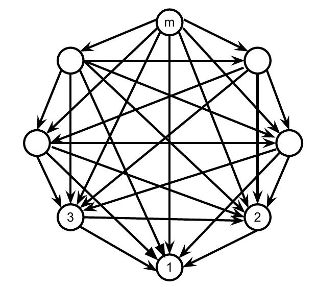
Figure 1: A complete DAG with $p$ vertices.

Before specifying our distribution on $\Theta_{\mathcal{D}}$, let us show that the same process is followed with the Cholesky decomposition of the $\mathrm{IW}_{\mathrm{P}_{\mathcal{G}}}$ in [16]. Let $\mathcal{G}$ be a decomposable or complete graph. Let $\mathcal{D}$ be its perfect Markov equivalent DAG. We consider the Gaussian model Markov with respect to $\mathcal{G}$ with covariance matrix $\Sigma$ and let us assume that $\Sigma^{-1}\sim\rm{W}_{\mathrm{P}_{\mathcal{G}}}(U,\alpha)$ or equivalently that $\Sigma\sim\mathrm{IW}_{\mathrm{P}_{\mathcal{G}}}(\alpha,U)$. We will let $(C_{1},C_{2},\ldots,C_{k})$ be a perfect order of $\mathcal{G}$ and $S_{j}$, j=2,…,k, be the minimal separators. We use the notation

$$H_{j}=C_{1}\cup\cdots\cup C_{j},\>\>R_{j}=C_{j}\setminus H_{j-1},\>\text{and}\>\>S_{j}=H_{j-1}\cap C_{j},$$

for $j=2,\ldots,k$, $R_{0}=S_{2}$, $R_{1}=C_{1}\setminus C_{2}$, $S_{0}=\emptyset$ and $S_{1}=S_{2}$. By Theorem 4.4 in [16], under the mapping $\Sigma\mapsto\times_{j=0}^{k}\left(\Sigma_{R_{j}|S_{j}},\Sigma_{S_{j}}^{-1}\Sigma_{S_{j}R_{j}}\right)$, the density of $\Sigma\sim\mathrm{IW}_{\mathrm{P}_{\mathcal{G}}}(\alpha,U)$ is transformed to a density proportional to

$$\exp\left\{-\frac{1}{2}\sum_{j=0}^{k}\left(\Sigma_{R_{j}|S_{j}}^{-1}(\Sigma_{S_{j}}^{-1}\Sigma_{S_{j}R_{j}}+U_{S_{j}}^{-1}U_{S_{j}R_{j}}\right)^{\top}U_{S_{j}}\left(\Sigma_{S_{j}}^{-1}\Sigma_{S_{j}R_{j}}+U_{S_{j}}^{-1}U_{S_{j}R_{j}})\right)\right\}$$

$$\times\prod_{j=0}^{k}\exp\left\{-\frac{1}{2}\Sigma_{R_{j}|S_{j}}^{-1}U_{R_{j}|S_{j}}\right\}\Sigma_{R_{j}|S_{j}}^{-\alpha_{j}/2}.$$ (7)

A close inspection of (3.1) shows that it is the image of (6) under the mapping $(D,L)\mapsto\times_{i\in V}\left(\lambda_{i},\beta_{\prec i]}\right)$ for a perfect DAG version $\mathcal{D}$ of $\mathcal{G}$, where $k+1$ shape parameters are introduced, one for each block $C_{1}\setminus S_{2}$, $S_{2}$, $R_{2},\ldots,R_{k}$. To see this, one can check (or see Supplemental section B subsection 2.2) that the image of (6) under the mapping $(D,L)\mapsto\times_{i\in V}\left(\lambda_{i},\beta_{\prec i]}\right)$ is written as

$$\exp\left\{-\frac{1}{2}\sum_{i=1}^{p}\Sigma_{ii|\prec i\succ}^{-1}(\Sigma^{-1}_{\prec i\succ}\Sigma_{\prec i]}-U^{-1}_{\prec i\succ}U_{\prec i]})^{\top}U_{\prec i\succ}(\Sigma^{-1}_{\prec i\succ}\Sigma_{\prec i]}-U^{-1}_{\prec i\succ}U_{\prec i]})\right\}$$

$$\prod_{i=1}^{p}\exp\left\{\Sigma_{ii|\prec i\succ}^{-1}U_{ii|\prec i\succ}\right\}\Sigma_{ii|\prec i\succ}^{-\frac{1}{2}\alpha_{i}}.$$ (8)

Although the number of shape parameters in (3.1) is less than that of (3.1) it is clear that by splitting the blocks $C_{1}\setminus S_{2},S_{2},R_{2},\ldots,R_{k}$ into vertices we can completely liberate the shape parameters by introducing one for each vertex. Once (3.1) is folded back to $\mathrm{P}_{\mathcal{D}}$ we obtain a multi-shape parameter density on $\mathrm{P}_{\mathcal{D}}$, which of course requires using the Jacobian of the corresponding mapping. We should however emphasize that a distribution of type (3.1) cannot be derived from the Type II Wishart distribution in [16] when $\mathcal{D}$ is an arbitrary DAG because $\rm{W}_{\mathrm{P}_{\mathcal{G}}}$ is derived as the natural exponential family generated by an appropriate measure on $\mathrm{P}_{\mathcal{G}}$, a machinery which cannot be employed if DAGs are not perfect. In spite of this, we can see that the transformed density (3.1) obtained in [16] can be generalized to the form of multi-shape parameter distribution (3.1) on $\Xi_{\mathcal{D}}$, and therefore $\Theta_{\mathcal{D}}$ for all DAGs. In addition, the form of density in (3.1) shows that the obtained distribution on $\Theta_{\mathcal{D}}$ has the strong hyper Markov property, which reiterates the statement of Theorem 4.4 [16] as

$$D_{ii}=\Sigma_{ii|\prec i\succ} \sim IG(\frac{\alpha_{i}}{2}-\frac{pa_{i}}{2}-1,\frac{1}{2}U_{ii|\prec i\succ}),~{}\text{and}$$ (9)

$$\Sigma_{\prec i\succ}^{-1}\Sigma_{\prec i]}|D_{ii} \sim\rm{N}_{pa_{i}}(U^{-1}_{\prec i\succ}U_{\prec i]},D_{ii}U^{-1}_{\prec i\succ}).$$ (10)

To summarize, in light of (3.1), the form of density given by (3.1) is a natural choice of the multi-shape parameter Wishart distribution on $\Xi_{\mathcal{D}}$ for an arbitrary DAG $\mathcal{D}$. For this reason, we define (6), the image of (3.1), as the DAG-Wishart density $\pi_{U,\alpha}^{\Theta_{\mathcal{D}}}$ on the Cholesky space $\Theta_{\mathcal{D}}$. It remains to compute the normalizing constant of $\pi_{U,\alpha}^{\Theta_{\mathcal{D}}}$ by multiple integration of the non-normalized density in (3.1) and taking advantage of the strong hyper Markov property manifested by (9) and (10). The calculation yields:

$$\pi_{U,{\bf\alpha}}^{\Theta_{\mathcal{D}}}(D,L) =\frac{1}{z_{\mathcal{D}}(U,{\bf\alpha})}\exp\left\{-\frac{1}{2}\mathrm{tr}((LD^{-1}L^{\top})U)\right\}\prod_{i=1}^{p}D^{-\frac{1}{2}\alpha_{i}}_{ii},$$

for $(D,L)\in\Theta_{\mathcal{D}}$ and

$$z_{\mathcal{D}}(U,\alpha)=\prod_{i=1}^{p}\frac{\Gamma\left(\frac{\alpha_{i}}{2}-\frac{pa_{i}}{2}-1\right)2^{\frac{\alpha_{i}}{2}-1}(\sqrt{\pi})^{pa_{i}}\det(U_{\prec i\succ})^{\frac{\alpha_{i}}{2}-\frac{pa_{i}}{2}-\frac{3}{2}}}{\det(U_{\preceq i\succeq})^{\frac{\alpha_{i}}{2}-\frac{pa_{i}}{2}-1}}.$$ (11)

Note that $\pi_{U,\alpha}^{\Theta_{\mathcal{D}}}$ is a conjugate prior for $\mathscr{N}(\mathcal{D})$. More precisely, if the prior distribution on $(D,L)$ is $\pi_{U,\alpha}^{\Theta_{\mathcal{D}}}$ and ${\bf Y}_{1},{\bf Y}_{2},\cdots,{\bf Y}_{n}$ is an independent and identically distributed sample from $\rm{N}_{p}({\bf 0},(L^{\top})^{-1}DL^{-1})$, then the posterior distribution of $(D,L)$ is given by $\pi_{\widetilde{U},\widetilde{\bf\alpha}}^{\Theta_{\mathcal{D}}}$, where $S=\frac{1}{n}\sum_{i=1}^{n}{\bf Y}_{i}{\bf Y}_{i}^{\top}$ denotes the empirical covariance matrix, $\widetilde{U}=nS+U$ and $\widetilde{\bf\alpha}=(n+\alpha_{1},n+\alpha_{2},\cdots,n+\alpha_{p})$.

Remark 3.1.

We note that parameterizing each $\pi_{U,\alpha}^{\Theta_{\mathcal{D}}}$ by parameter $U\succ 0$ is not an identifiable parameterization, since the mapping $U\mapsto\pi_{U,\alpha}^{\Theta_{\mathcal{D}}}$ is not one-to-one, unless $\mathcal{D}$ is a perfect DAG. However, if the parameter set is restricted to $\mathrm{PD}_{\mathcal{D}}$, then the parameterization is identifiable. As a parameterized model, $\{\pi_{U,\alpha}^{\Theta_{\mathcal{D}}}:\>U\in\mathrm{PD}_{\mathcal{D}}\}$ is in general a curved exponential family for an arbitrary DAG $\mathcal{D}$, and a natural exponential family if and only if $\mathcal{D}$ is perfect (see Supplemental section B section 2.7 for details).

4 The DAG-Wishart distribution on the space of incomplete precision matrices

In the previous section we introduced the DAG-Wishart distribution $\pi^{\Theta_{\mathcal{D}}}_{U,\alpha}$ on the Cholesky space $\Theta_{\mathcal{D}}$. In this section we proceed to define, for general DAGs, an analog of the type II Wishart defined in [16] for decomposable (or complete) graphs.

4.1 Motivation and notation

To follow in the tradition of the Wishart, the inverse hyper inverse Wishart and the type II Wishart mentioned above, we would like to derive a type of Wishart distribution for the covariance and precision matrices of $N(0,\Sigma)\in{\cal N}_{\mathcal{D}}$, that is, we would like to derive the image of the $\pi^{\Theta_{\mathcal{D}}}_{U,\alpha}$ distribution under the mappings

$$\left((D,L)\mapsto LD^{-1}L^{\top}\right) :\Theta_{\mathcal{D}}\rightarrow\mathrm{P}_{\mathcal{D}}$$ (12)

$$\left((D,L)\mapsto\left(LD^{-1}L^{\top}\right)^{-1}\right) :\Theta_{\mathcal{D}}\rightarrow\mathrm{PD}_{\mathcal{D}}.$$ (13)

The main issue, as we elaborate in Supplemental section C, is that these image distributions have no densities with respect to the Lebesgue measure if $\mathcal{D}$ is not perfect. This problem arises because both the space of precision and covariance matrices have Lebesgue measure zero in their affine supports. From a purely mathematical or theoretical point of view, one can derive the densities with respect to Hausdorff measure. But even for the simplest DAGs, the Hausdorff density is not amenable to posterior analysis (see Supplemental section C for a more detailed discussion of this approach).

To overcome this problem, we follow what was done for the hyper inverse Wishart in [15] or for the type I Wishart in [16] and we work with the projections of $\mathrm{P}_{\mathcal{D}}$ and $\mathrm{PD}_{\mathcal{D}}$ onto the Euclidean space that only retain the functionally independent elements of the precision and covariance matrices of Gaussian DAG models.

The projected spaces, as we shall see, are subsets of incomplete matrices, which we call the incomplete precision space $\mathrm{R}_{\mathcal{D}}$ and the incomplete covariance space $\mathrm{S}_{\mathcal{D}}$, respectively. The precise definitions are as follows.

Definition 4.1.

Let $\mathcal{D}=(V,E)$ be a DAG and $\mathcal{D}^{u}=(V,E^{u})$ its undirected version.

• Let $\mathrm{Z}_{\mathcal{D}}\subseteq\mathbb{R}^{p\times p}$ denote the real linear space of $p\times p$ symmetric matrices $A$ such that $A_{ij}=A_{ji}=0$ if $(i,j)$ is not in $E$. Note that the dimension of $\mathrm{Z}_{\mathcal{D}}$ is $|E|$.

• Let $\mathrm{I}_{\mathcal{D}}$ denote the real linear space of symmetric functions $\Gamma=\left(\Gamma_{ij}\right)_{(i,j)\in E^{u}}$, i.e., $\Gamma_{ij}=\Gamma_{ji}\in\mathbb{R}$ for each $(i,j)\in E$. An element $\Gamma\in\mathrm{I}_{\mathcal{D}}$ is called a (symmetric) $\mathcal{D}$-incomplete matrix, and can be considered as a matrix in $\mathrm{S}_{p}(\mathbb{R})$ where only the entries corresponding to the edges of $\mathcal{D}$ are specified and the rest are unspecified. The projection mapping from $\mathrm{S}_{p}(\mathbb{R})$ onto $\mathrm{I}_{\mathcal{D}}$ is denoted by $A\mapsto A^{E}$

• For $\Gamma\in\mathrm{I}_{\mathcal{D}}$ let $\left(\Gamma\right)^{0}$ denote the $|V|\times|V|$ matrix

  $$\left(\Gamma\right)^{0}_{ij}=\begin{cases}\Gamma_{ij}&\text{ if $(i,j)\in E^{u}$},\\ 0&\text{otherwise.}\end{cases}$$

Note that $\left(\Gamma\right)^{0}$ fills or completes the unspecified positions with zeros to obtain a full matrix in $\mathrm{Z}_{\mathcal{D}}$. For each clique $c$ of $\mathcal{D}$ the restriction of $\Gamma$ on $c$, denoted by $\Gamma_{c}$, is a full matrix. Moreover, $\Gamma$ is uniquely determined by the blocks of matrices $(\Gamma_{c}:c\in\mathscr{C}_{\mathcal{D}})$, where $\mathscr{C}_{\mathcal{D}}$ denotes the set of cliques of $\mathcal{D}^{u}$.

• Let $\mathrm{Q}_{\mathcal{D}}\subseteq\mathrm{I}_{\mathcal{D}}$ denote the set of $\mathcal{D}$-incomplete matrices $\Gamma\in\mathrm{I}_{\mathcal{D}}$ such that $\Gamma_{c}$ is positive definite for each clique $c\in\mathscr{C}_{\mathcal{D}}$. Each element of $\mathrm{Q}_{\mathcal{D}}$ is said to be a partially positive definite matrix over $\mathcal{D}$.

• Let $\mathcal{A}\subseteq\mathrm{S}_{p}(\mathbb{R})$. We say that a $\mathcal{D}$-incomplete matrix $\Gamma\in\mathrm{I}_{\mathcal{D}}$ can be completed in $\mathcal{A}$ if there exists a matrix $A\in\mathcal{A}$ such that $A_{ij}=\Gamma_{ij}$ for each $(i,j)\in E$, i.e., $A^{E}=\Gamma$. We refer to $A$ as a completion of $\Gamma$ in $\mathcal{A}$.

• The space of incomplete precision matrices over $\mathcal{D}$, denoted by $\mathrm{R}_{\mathcal{D}}$, is the set of $\Gamma\in\mathrm{I}_{\mathcal{D}}$ that can be completed in the space of precision matrices $\mathrm{P}_{\mathcal{D}}$.

• The space of incomplete covariance matrices over $\mathcal{D}$, denoted by $\mathrm{S}_{\mathcal{D}}$, is the set of $\Upsilon\in\mathrm{I}_{\mathcal{D}}$ that can be completed in the space of covariance matrices $\mathrm{PD}_{\mathcal{D}}$.

Remark 4.1.

If $\mathcal{A}$ is the set of positive definite matrices $\mathrm{PD}_{p}(\mathbb{R})$, then the completion in $\mathcal{A}$ reduces to the standard definition of positive definite completion [10]. We shall consider below the positive definite completion of partially positive precision/covariance matrices that correspond to DAGs (vs. those that correspond to undirected graphs as in [10]). Note that an incomplete matrix $\Gamma\in\rm{I}_{\mathcal{D}}$ has a positive definite completion only if $\Gamma\in\mathrm{Q}_{\mathcal{D}}$, i.e., it is partially positive definite over $\mathcal{D}$.

4.2 The space of incomplete precision matrices

We first recall the definition of $\mathrm{R}_{\mathcal{D}}$ in Definition 4.1 and the following result from [2].

Proposition 4.1.

[2] Let $\Gamma$ be a $\mathcal{D}$-partial matrix in $\mathrm{I}_{\mathcal{D}}$. If  $\Gamma_{11}\neq 0$, then

• Almost everywhere (with respect to the Lebesgue measure on $\mathrm{I}_{\mathcal{D}}$), there exist a unique lower triangular matrix $L\in\mathcal{L}_{\mathcal{D}}$ and a unique diagonal matrix $\Lambda\in\mathbb{R}^{p\times p}$ such that $\widehat{\Gamma}=L\Lambda L^{\top}$ is a completion of $\Gamma$.

• The matrix $\widehat{\Gamma}$ is the unique positive definite completion of $\Gamma$ in $\mathrm{P}_{\mathcal{D}}$ if and only if the diagonal entries of $\Lambda$ are all strictly positive.

Proposition 4.1 is of interest to us, because it explicitly shows that without loss of generality every precision matrix $\Omega\in\mathrm{P}_{\mathcal{D}}$ can be represented by a $\mathcal{D}$-incomplete matrix which only consists of the free parameters of $\Omega$, i.e., $\Omega^{E}$. The rest, entries corresponding to the missing edges of the DAG, can be discarded, as whenever needed they can be obtained from $\Omega^{E}$ according to a constructive completion procedure given by the proof of Proposition 4.1. We re-formalize this as follows.

Corollary 1.

The projection mapping $\left(\Omega\mapsto\Omega^{E}\right):P_{\mathcal{D}}\rightarrow\mathrm{R}_{\mathcal{D}}$ is a homeomorphism with the inverse mapping $\left(\Upsilon\mapsto\widehat{\Upsilon}\right):\mathrm{R}_{\mathcal{D}}\rightarrow\mathrm{P}_{\mathcal{D}}$.

4.3 The DAG-Wishart distribution on $\mathrm{R}_{\mathcal{D}}$

In light of Corollary 1 we identify $\mathrm{P}_{\mathcal{D}}$ with $R_{\mathcal{D}}$ through the bijection $\Omega\mapsto\Omega^{E}$. Note that $\mathrm{R}_{\mathcal{D}}$, unlike $\mathrm{P}_{\mathcal{D}}$, is open in its affine support $\mathrm{I}_{\mathcal{D}}$ and, as a consequence of Corollary 1, homeomorphic to $\Theta_{\mathcal{D}}$. Recall that we refer to $\mathrm{R}_{\mathcal{D}}$ as the space of incomplete precision matrices over $\mathcal{D}$. Now let $\pi_{U,\alpha}^{\mathrm{R}_{\mathcal{D}}}$ denote the image of $\pi^{{\Theta}_{\mathcal{D}}}_{U,\alpha}$ under the mapping

$$\psi\equiv\left(\left(L,D\right)\mapsto\left(LD^{-1}L^{t}\right)^{E}\right):\Theta_{\mathcal{D}}\rightarrow\mathrm{R}_{\mathcal{D}}$$ (14)

Since $\mathrm{R}_{\mathcal{D}}$ is an open subset of the Euclidean space $\mathbb{R}^{|E|}$, the distribution $\pi_{U,\alpha}^{\mathrm{R}_{\mathcal{D}}}$ has a density with respect to the Lebesgue measure on $\mathrm{R}_{\mathcal{D}}$. Hence, in light of the homeomorphism $\Omega\mapsto\Omega^{E}$, in both a natural and practical sense, we define $\pi_{U,\alpha}^{\mathrm{R}_{\mathcal{D}}}$ as the DAG-Wishart distribution on the space of incomplete precision matrices $\mathrm{R}_{\mathcal{D}}$. To derive the density of $\pi_{U,\alpha}^{\mathrm{R}_{\mathcal{D}}}$ we need to compute the Jacobian of the mapping $\psi$ in (14). The Jacobian of $\psi$ is a variant of similar transformations found in [19, 14]. For completeness we still compute this Jacobian in the following lemma. The proof is given in Supplemental section B subsection 2.7.

Lemma 4.2.

[19, 14] The Jacobian of the mapping $\psi:(D,L)\mapsto\left(LD^{-1}L^{\top}\right)^{E}$ is $\prod_{j=1}^{p}D_{jj}^{-(pa_{j}+2)}$.

We now proceed to express the density of $\pi_{U,\alpha}^{\mathrm{R}_{\mathcal{D}}}$ and some of its properties. The proofs are immediate results of Lemma 7.8 and the iterative construction of $\pi^{\Theta_{\cal D}}_{U,\alpha}$.

Theorem 4.3.

Let $\Upsilon$ be the image of $\left(L,D\right)\sim\pi_{U,\alpha}^{\Theta_{\mathcal{D}}}$ under the mapping $\psi$. Then

• The density of $\Upsilon\sim\pi^{\mathrm{R}_{\mathcal{D}}}_{U,\alpha}$ with respect to the standard Lebesgue measure on $\mathrm{R}_{\mathcal{D}}$ is given by

  $$z_{\mathcal{D}}(U,\alpha)^{-1}\exp\left\{-\frac{1}{2}\mathrm{tr}(\widehat{\Upsilon}U)\right\}\prod_{i=1}^{p}D_{ii}^{-\frac{1}{2}\alpha_{i}+pa_{i}+2},$$

  where $D_{ii}=\left(\widehat{\Upsilon}^{-1}\right)_{ii|\prec i\succ}$ is explicitly a function of $\Upsilon$ and $z_{\mathcal{D}}$ is defined in (11).

• The Laplace transform of $\pi^{\mathrm{R}_{\mathcal{D}}}_{U,\alpha}$ at $K^{E}$ is given by $\mathcal{L}_{R_{\mathcal{D}}}(K^{E})=\displaystyle\frac{z_{\mathcal{D}}(2K+U,\alpha)}{z_{\mathcal{D}}(U,\alpha)}$.

• $\mathbb{E}\left(\Upsilon\right)=\left(\sum^{p}_{j=1}(\alpha_{j}-pa_{j}-2)\left(U^{-1}_{\preceq j\succeq}\right)^{0}-\sum^{p}_{j=1}(\alpha_{j}-pa_{j}-3)\left(U^{-1}_{\prec j\succ}\right)^{0}\right)^{E}$.

Figure 2: A directed 4-cycle.

Ex 4.1.

Let $\mathcal{D}$ be the DAG given by Figure 2. Then the DAG-Wishart density $\pi_{U,\alpha}^{\mathrm{R}_{\mathcal{D}}}$ is given by

where, using Proposition 4.1, $\widehat{\Upsilon}$ and $D_{ii}\left(\Upsilon\right)$ are computed as follows.

5 The inverse DAG-Wishart distribution on the space of incomplete covariance matrices

In this section, we shall define the distribution that corresponds to the hyper-inverse Wishart or more generally the inverse Type II Wishart $\mathrm{IW}_{\mathrm{P}_{\mathcal{G}}}$. We therefore call it the inverse ${\mathcal{D}}$-Wishart or inverse DAG-Wishart distribution. First we introduce the space of incomplete covariance matrices. We recall two important propositions from [2] for completing an incomplete matrix in the space of covariance or inverse covariance matrices. We use these theorems later for parameter estimation and model selection.

5.1 The space of incomplete covariance matrices

Recall that $\mathrm{PD}_{\mathcal{D}}$ is the space of covariance matrices for the Gaussian DAG model $\mathscr{N}(\mathcal{D})$, the elements of which, according to (3), can be characterized as:

$$\Sigma\in\mathrm{PD}_{\mathcal{D}}\Longleftrightarrow\Sigma\succ 0\>\>\&\>\>\Sigma_{[i\nsucc}=\Sigma_{[i\succ}\Sigma_{\prec i\succ}^{-1}\Sigma_{\prec i\nsucc},\>\text{for each $i\in V$}.$$ (15)

The above characterization allows us to identify $\mathrm{PD}_{\mathcal{D}}$ with the functionally independent elements of $\Sigma$. The following proposition is a key ingredient in this identification.

Proposition 5.1.

[2] Let $\Gamma\in\mathrm{Q}_{\mathcal{D}}$, then

1. There exists a completion process of polynomial complexity that can determine whether $\Gamma$ can be completed in $\mathrm{PD}_{\mathcal{D}}$;

2. If a completion exists, this completion is unique and can be determined constructively using the following process:

   • Set $\Sigma_{ij}=\Gamma_{ij}$   for each $(i,j)\in E$ and set $j=p$.

   • If $j>1$, then set $j=j-1$ and proceed to the next step, otherwise $\Sigma$ is successfully completed.

   • If $\Sigma_{\preceq j\succeq}>0$, then proceed to the next step, otherwise the completion in $\mathrm{PD}_{\mathcal{D}}$ does not exist.

   • If $\Sigma_{\nprec j]}$ is non-empty, then set $\Sigma_{\nprec j]}=\Sigma_{\nprec j\succ}\Sigma_{\prec j\succ}^{-1}\Sigma_{\prec j]},$ $\Sigma_{[j\nsucc}=\Sigma_{\nprec j]}^{t}$ and return to step $(2).$

Remark 5.1.

Note once more that the procedure in Proposition 5.1 itself determines if $\Gamma$ can be completed in $\mathrm{PD}_{\mathcal{D}}$. It is clear from Step (iii) above that the necessary and sufficient condition for the existence of a positive definite completion is that, for each $j\in V$, the covariance sub-matrix $\Sigma_{\preceq j\succeq}>0$ and not just $\Sigma_{\prec j\succ}>0$. Furthermore, the completion procedure in Proposition 5.1 can terminate midway.

From Definition 4.1 recall that $\mathrm{S}_{\mathcal{D}}$ denotes the set of $\Gamma\in\mathrm{I}_{\mathcal{D}}$ that can be completed in $\mathrm{PD}_{\mathcal{D}}$. We call this set the space of incomplete covariance matrices over $\mathcal{D}$. The next corollary formalizes the fact that $\mathrm{S}_{\mathcal{D}}$ can be identified with $\mathrm{PD}_{\mathcal{D}}$. Its proof is immediate from Proposition 5.1 above.

Corollary 2.

The mapping $(\Sigma\mapsto\Sigma^{E}):\mathrm{PD}_{\mathcal{D}}\rightarrow\mathrm{S}_{\mathcal{D}}$ is a bijection with inverse mapping $\Gamma\mapsto\Sigma$, where $\Sigma=\widetilde{\Gamma}$ is the completion matrix constructed according to Proposition 5.1.

Remark 5.2.

Suppose $\mathcal{D}$ is perfect. Then $\mathrm{PD}_{\mathcal{D}}$ is identical to $\mathrm{PD}_{\mathcal{D}^{\mathrm{u}}}$ and, therefore, by the completion result in Grone et al. [10], every incomplete matrix in $\mathrm{Q}_{\mathcal{D}}$ can be completed in $\mathrm{PD}_{\mathcal{D}}$. Hence for $\mathcal{D}$ perfect, $\mathrm{S}_{\mathcal{D}}$ and $\mathrm{Q}_{\mathcal{D}}$ are identical.

5.2 The inverse DAG-Wishart distribution on $\mathrm{S}_{\mathcal{D}}$

Let $\pi_{U,\alpha}^{\mathrm{S}_{\mathcal{D}}}$ denote the image of $\pi_{U,\alpha}^{\Theta_{\mathcal{D}}}$ under the mapping $(D,L)\mapsto(L^{-t}DL^{\top})^{E}:\Theta_{\mathcal{D}}\rightarrow\mathrm{S}_{\mathcal{D}}$, where $L^{-t}=\left(L^{\top}\right)^{-1}$. In parallel to our notation $\pi_{U,\alpha}^{\mathrm{R}_{\mathcal{D}}}$, we will denote the inverse DAG-Wishart distribution on the space of incomplete covariance matrices $\mathrm{S}_{\mathcal{D}}$ as $\pi_{U,\alpha}^{\mathrm{S}_{\mathcal{D}}}$. Next we shall derive the density of this distribution with respect to the Lebesgue measure. First we compute the Jacobian of the mapping $(\Sigma^{E}\mapsto\Sigma^{-E}):\mathrm{S}_{\mathcal{D}}\rightarrow\mathrm{R}_{\mathcal{D}}$, where $\Sigma^{-E}=\left(\Sigma^{-1}\right)^{E}$ and $\Sigma$ is the completion of $\Sigma^{E}$ in $\mathrm{PD}_{\mathcal{D}}$.

Lemma 5.2.

Let $\mathcal{D}=(V,E)$ be an arbitrary DAG, then the Jacobian of the mapping $(\Sigma^{-E}\mapsto\Sigma^{E}):\mathrm{R}_{\mathcal{D}}\rightarrow\mathrm{S}_{\mathcal{D}}$ is given by $\prod_{i=1}^{p}\displaystyle\frac{\det\Sigma_{\preceq i\succeq}^{pa_{i}+2}}{\det\Sigma_{\prec i\succ}^{pa_{i}+1}}$.

Proof: First note that the mapping $\Sigma^{-E}\mapsto\Sigma^{E}$ can be written as the composition of the two mappings

$$(\Sigma^{-E}\mapsto\times_{i=1}^{p}(\Sigma_{ii|\prec i\succ},\Sigma_{\prec i\succ}^{-1}\Sigma_{\prec i]}):\mathrm{R}_{\mathcal{D}}\rightarrow\Xi_{\mathcal{D}};$$

$$(\times_{i=1}^{p}(\Sigma_{ii|\prec i\succ},\Sigma_{\prec i\succ}^{-1}\Sigma_{\prec i]})\mapsto\Sigma^{E}):\Xi_{\mathcal{D}}\rightarrow\mathrm{S}_{\mathcal{D}}.$$

It is easy to check that the Jacobian of the first mapping is the same as the Jacobian of the inverse of the mapping $\psi:(L,D)\mapsto(LD^{-1}L^{t})^{E}$ in Lemma 7.8 and is therefore equal to $\prod_{i=1}^{p}\Sigma_{ii|\prec i\succ}^{pa_{i}+2}$.

We shall proceed by mathematical induction to compute the Jacobian of the second mapping. Let us assume that the Jacobian of the mapping

$$(\times_{i=1}^{p}(\Sigma_{ii|\prec i\succ},\Sigma_{\prec i\succ}^{-1}\Sigma_{\prec i]})\mapsto\Sigma^{E}):\Xi_{\mathcal{D}}\rightarrow\mathrm{S}_{\mathcal{D}}$$

is equal to $\prod_{i=1}^{|V|}\det(\Sigma_{\prec i\succ})$ for any DAG $\mathcal{D}$ with $|V|<p$. We will show that the result will also hold true for $|V|=p$. The case $p=1$ is trivial. So assume that $p\geq 2$. Let $\mathcal{D}_{[1]}$ be the induced subgraph of $\mathcal{D}$ with the vertex set $V_{[1]}=V\setminus\left\{1\right\}$ and the corresponding edge set, denoted by $E_{[1]}$. Since $V_{[1]}$ is an ancestral subset of $V$, if $\Sigma^{E}$ belongs to $\mathrm{S}_{\mathcal{D}}$, then $\Sigma^{E_{[1]}}$, the projection of $\Sigma$ on $I_{G_{[1]}}$, is an element of $\mathrm{S}_{\mathcal{D}_{[1]}}$. Furthermore the positive definite completion of in $\mathrm{PD}_{\mathcal{D}_{[1]}}$ is indeed the principal sub-matrix $\Sigma_{V_{[1]}}$. The above two observations simply follow from the recursive nature of the completion process in Proposition 5.1. Now consider the following composition of the inverse mapping $\Sigma^{E}\mapsto\times_{i=1}^{p}(\Sigma_{ii|\prec i\succ},\Sigma_{\prec i\succ}^{-1}\Sigma_{\prec i]})$

$$\begin{array}[]{lrlll}\mathrm{S}_{\mathcal{D}}&\rightarrow&\mathbb{R}_{+}\times\mathbb{R}^{\prec 1]}\times\mathrm{S}_{\mathcal{D}_{[1]}}&\rightarrow&\mathbb{R}_{+}\times\mathbb{R}^{\prec 1]}\times\Xi_{\mathcal{D}_{[1]}}=\Xi_{\mathcal{D}}\\ \Sigma^{E}&\mapsto&(\Sigma_{11|\prec 1\succ},\Sigma_{\prec 1\succ}^{-1}\Sigma_{\prec 1]},\Sigma^{E_{[1]}})&\mapsto&\left(\Sigma_{11|\prec 1\succ},\Sigma_{\prec 1\succ}^{-1}\Sigma_{\prec 1]},\times_{i=2}^{p}(\Sigma_{ii|\prec i\succ},\Sigma_{\prec i\succ}^{-1}\Sigma_{\prec i]})\right)\end{array}$$

By the inductive hypothesis the Jacobian of the second mapping,

$$(\Sigma_{11|\prec 1\succ},\Sigma_{\prec 1\succ}^{-1}\Sigma_{\prec 1]},\Sigma^{E_{[1]}})\mapsto\left(\Sigma_{11|\prec 1\succ},\Sigma_{\prec 1\succ}^{-1}\Sigma_{\prec 1]},\times_{i=2}^{p}(\Sigma_{ii|\prec i\succ},\Sigma_{\prec i\succ}^{-1}\Sigma_{\prec i]})\right),$$

is equal to $\prod_{i=2}^{p}\det(\Sigma_{\prec i\succ})^{-1}$. Hence it suffices to prove that the Jacobian of the first mapping, $\Sigma^{E}=(\Sigma_{11},\Sigma_{\prec 1]},\Sigma^{E_{[1]}})\mapsto(\Sigma_{11|\prec 1\succ},\Sigma_{\prec 1\succ}^{-1}\Sigma_{\prec 1]},\Sigma^{E_{[1]}})$ is $\det(\Sigma_{\prec 1\succ})^{-1}$. This follows by noting that the Jacobian matrix of this mapping is lower triangular and is given as follows:

$$\left(\begin{matrix}I&0&0\\ *&\Sigma_{\prec 1\succ}^{-1}&0\\ *&*&1\end{matrix}\right)$$

The results now follows by induction.

We now proceed to state the functional form of the density of $\pi_{U,\alpha}^{\mathrm{S}_{\mathcal{D}}}$ with respect to Lebesgue measure.

Corollary 3.

Let $\Sigma\sim\pi_{U,\alpha}^{\mathrm{PD}_{\mathcal{D}}}$ and let $\Gamma=\Sigma^{E}$, i.e., $\Sigma$ is the completion of $\Gamma$ in $\mathrm{PD}_{\mathcal{D}}$. Then the density of $\Gamma\sim\pi_{U,\alpha}^{\mathrm{S}_{\mathcal{D}}}$ with respect to Lebesgue measure is given by

$$z_{\mathcal{D}}(U,\alpha)^{-1}\exp\left\{-\frac{1}{2}\mathrm{tr}(\Sigma^{-1}U)\right\}\prod_{i=1}^{p}\displaystyle\frac{\det\Sigma_{\preceq i\succeq}^{-\frac{1}{2}\alpha_{i}}}{\det\Sigma_{\prec i\succ}^{-\frac{1}{2}\alpha_{i}+1}}.$$ (16)

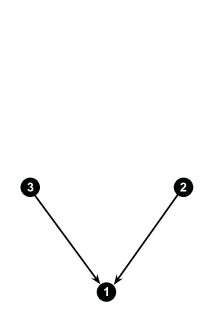
Figure 3: DAG studied in example 5.1

Ex 5.1.

Consider the DAG $\mathcal{D}$ given in Figure 3. Then the inverse DAG-Wishart on $\mathcal{D}$ is given by

$$\pi_{U,\alpha}^{\mathrm{S}_{\mathcal{D}}}(\Gamma)=z_{\mathcal{D}}(U,\alpha)^{-1}\exp\left\{-\frac{1}{2}\mathrm{tr}(\Sigma^{-1}U)\right\}D^{-\frac{1}{2}\alpha_{1}}_{11}D_{22}^{-\frac{1}{2}\alpha_{2}}D_{33}^{-\frac{1}{2}\alpha_{3}}\det(\Sigma_{\prec 1\succ})^{-1},$$

where $\Sigma$, the completion of $\Gamma$, is simply computed as

$$\Sigma=\begin{pmatrix}\Gamma_{11}&\Gamma_{12}&\Gamma_{13}\\ \Gamma_{21}&\Gamma_{22}&0\\ \Gamma_{31}&0&\Gamma_{33}\end{pmatrix}.$$

Remark 5.3.

We remind the reader that for a decomposable graph $\mathcal{G}$ the inverse Type II Wishart in [16] is a variant of $\pi^{\mathrm{S}_{\mathcal{D}}}_{U,\alpha}$ for a perfect DAG version of $\mathcal{G}$. Furthermore, in the setting of Gaussian covariance graph models, the inverse Wishart distribution introduced by Khare and Rajaratnam [14] for a homogeneous graph $\mathcal{G}$ is an equivalent form of $\pi^{\mathrm{S}_{\mathcal{D}}}_{U,\alpha}$ for a transitive and perfect DAG version $\mathcal{D}$ of $\mathcal{G}$. The proof of this result is rather technical and is given in Supplemental section B subsection 2.9.

5.3 Properties of the inverse DAG-Wishart distributions

One of the main useful properties of the inverse DAG-Wishart $\pi_{U,\alpha}^{\mathrm{S}_{\mathcal{D}}}$ for an arbitrary DAG is their strong hyper Markov properties. As discussed in section 3.1, this follows directly from Theorem 4.4 in [16] but is generalized to arbitrary DAGs. The precise statement of the strong hyper Markov property for $\pi_{U,\alpha}^{\mathrm{S}_{\mathcal{D}}}$ is as follows.

Theorem 5.3.

If  $\Sigma^{E}\sim{\pi}_{U,\alpha}^{\mathrm{S}_{\mathcal{D}}}$, then
$i)$  $\left\{(\Sigma_{ii|\prec i\succ},\Sigma_{\prec i\succ}^{-1}\Sigma_{\prec i]}:i\in V\right\}$ are mutually independent and therefore ${\pi}^{\mathrm{S}_{\mathcal{D}}}_{U,\alpha}$ is strongly directed Markov.
$ii)$  The distribution of $\Sigma_{ii|\prec i\succ}$ and $\Sigma_{\prec i\succ}^{-1}\Sigma_{\prec i]}|\Sigma_{ii|\prec i\succ}$ are, respectively, given by

$$\Sigma_{ii|\prec i\succ}\sim IG(\frac{\alpha_{i}}{2}-\frac{pa_{i}}{2}-1,\frac{1}{2}U_{ii|\prec i\succ}),~{}\text{and}$$ (17)

$$\Sigma_{\prec i\succ}^{-1}\Sigma_{\prec i]}|\Sigma_{ii|\prec i\succ}\sim\rm{N}_{pa_{i}}(U^{-1}_{\prec i\succ}U_{\prec i]},\Sigma_{ii|\prec i\succ}U^{-1}_{\prec i\succ}).$$ (18)

We can also evaluate the expected value under $\pi_{U,\alpha}^{\mathrm{S}_{\mathcal{D}}}$. The process for computing this quantity, given in the following proposition, is the exact equivalent of Theorem 3.1 in [18] but now generalized so it is applicable to any DAGs.

Proposition 5.4.

Suppose $\Sigma^{E}\sim{\pi}^{\mathrm{S}_{\mathcal{D}}}_{U,\alpha},$ with $\alpha>pa_{i}+4$. Then the expected value of $\Sigma^{E}$ can be recursively computed by the following steps:
$(i)$ $\mathbb{E}\left(\Sigma_{pp}\right)=\displaystyle\frac{U_{pp}}{\alpha_{p}-4}$,
$(ii)$ $\mathbb{E}\left(\Sigma_{\prec i]}\right)=-\mathbb{E}\left(\Sigma_{\prec i\succ}\right)U^{-1}_{\prec i\succ}U_{\prec i]}$,
$(iii)$ $\mathbb{E}\left(\Sigma_{ii}\right)=\displaystyle\frac{U_{ii|\prec i\succ}}{\alpha_{i}-pa_{i}-4}+\mathrm{tr}\left(\mathbb{E}\left(\Sigma_{\prec i\succ}\right)\left(\displaystyle\frac{U_{ii|\prec i\succ}U^{-1}_{\prec i\succ}}{\alpha_{i}-pa_{i}-4}+U^{-1}_{\prec i\succ}U_{\prec i]}U_{[i\succ}U^{-1}_{\prec i\succ}\right)\right)$,
for $i=p-1$,$p-2,\ldots,1$.

6 Simulation study and Applications to real data

We will now illustrate the use of our DAG-Wishart distributions by applying them to two problems in modern high dimensional statistical inference. These are Bayesian model selection in the space of Gaussian DAG models with a given order of the vertices, and parameter estimation using the flexible DAG-Wishart priors respectively. Our Bayesian model selection method based on the DAG-Wishart prior admits a closed form marginal likelihood, and to our knowledge it thus is more scalable than previous Bayesian approaches (in our examples, we illustrate the model selection of graphs with as high as $p=2000$). The second problem is the estimation of the covariance and precision matrices corresponding to Gaussian DAG models. We illustrate the properties of our DAG-Wishart approach, such as closed form solutions for the estimates of the precision matrix, ease of implementation and scalability for model selection, using simulated data. In addition, we further illustrate its effectiveness by applying it to molecular network data.

6.1 Bayesian model selection via DAG-Wishart prior

In many applications, the graph structure is unknown beforehand and estimating an underlying graph is an important contemporary problem. In this section, we illustrate how to apply the DAG-Wishart priors to model selection problems. In a Bayesian search, to select a graph $\mathcal{D}$, we want to evaluate the posterior likelihood:

$$p(\mathcal{D}|\mathbf{X})\propto p(\mathbf{X}|\mathcal{D})p(\mathcal{D}).$$

Assuming a uniform prior on the space of all graphs on $p$ vertices, this is equivalent to computing the marginal likelihood

$$p(\mathbf{X}|\mathcal{D})=\int{f(\mathbf{X}|\Sigma,\mathcal{D})\pi(\Sigma|\mathcal{D})d\Sigma}.$$

The marginal likelihood can be computed in closed form for our flexible DAG Wishart priors. For a model search strategy, we propose an improved stochastic short-gun search (SSS) of [12] coupled with the LassoDAG method in [21]. Our model selection algorithm, DAG-W, is specified below:

Algorithm 4 (DAG-W).

Assume the following are given: the standardized data matrix $X$, the hyper-parameters $\alpha$, $U$ and the maximum iteration number $M$. Estimate $N$ models corresponding to different points on the LassoDAG regularization path, labeled as $\mathcal{D}^{(k)},k=1,\cdots,N$. Then for each $k=1,2,\cdots,N$, do the following.

1. Let $\mathcal{D}_{0}=\mathcal{D}^{(k)}$. Until the maximum iteration number $M$ is achieved:

   1. Select $N_{1}$ graphs that are one edge away from $\mathcal{D}_{0}$. Evaluate the $\log$ posterior scores $s_{1},\cdots,s_{N_{1}}$ for each of these graphs, according to the DAG-Wishart prior/posterior. Record all of these graphs and scores as a list $\mathcal{L}^{(k)}$.

   2. Sample the next graph from the current graph list with probability $p_{i}\propto\exp{(s_{i})}^{\gamma}$, where $\gamma$ is an annealing parameter. Take the sampled graph $\mathcal{D}_{new}$ as $\mathcal{D}_{0}$.

   3. Return to Step 1-(a).

2. Collect/Assemble all the $\mathcal{L}^{(k)},k=1,\cdots,N$.

3. Return the graph with the largest score as the selected model.

As indicated in the algorithm above, we take the various models corresponding to different penalty parameter values on the LassoDAG regularization path as our baseline models. In [21], the penalty parameter $\tau_{i}$ for the Lasso problem of node $i$ is set to

$$\tau_{i}=2\frac{Z^{*}_{\frac{\kappa}{2p(i-1)}}}{\sqrt{n}},$$ (19)

where in general $Z^{*}_{q}$ denotes the $(1-q)$th quantile of standard normal distribution and $\kappa=0.1$ is the recommended value in [21]. Here we use the same setup as in [21] to evaluate and compare the performance of the LassoDAG to our DAG-W algorithm. More details are as follows.

The scale parameter $U$ of the DAG-Wishart is taken to be the identity matrix. As in the covariance estimation section below, we constrain the shape parameters to be $c\cdot pa_{i}+b$ such that $c\cdot pa_{i}+b>pa_{i}+2$. In particular, we take $b=3,c=1$ in model selection as this seems to give reasonably good model selection results in all of our evaluation tasks (with different $p,n$ and sparsity). We set $N=16$ in Algorithm 4 for our Bayesian model selection: 15 initial states were chosen by taking $\kappa=(k/15)^{4}p,k=1\cdots 15$ in (19) and the sixteenth state was selected using the LassoDAG recommendation $\kappa=0.1$. Furthermore, we take $M=100$, $N_{1}=30$ and $\gamma=0.5$.

The data is generated by the random DAG generator in the R-package pcalg ([13], [11]). In our evaluation, we specify the edge proportion (sparsity) to be 0.01 in generating the DAG and the edge regression weights are uniformly sampled between 0.2 and 0.8. The reader is referred to pcalg documentation for details about the DAG model generating procedure. Fixing $n=100$, we check the model selection performance when the edge proportion is 0.01 and $p=50$, $100$, $200$, $500$, $1000$, $1500$ and $2000$. The performance is measured by two competing measurements: sensitivity and specificity, which are frequently used in model selection tasks (see [baldi2000assessing]). Sensitivity is used to measure the proportion of true edges discovered while specificity is used to measure the proportion of the null edges that are correctly excluded.

Table 1 shows the performance comparison between the Lasso-DAG and DAG-W. Both methods are able to retain very good specificity. The DAG-W gives much better sensitivity with only slightly lower specificity. When $p$ is large, the improvement in sensitivity is more stark. In the case of $p=2000$, the sensitivity given by the DAG-W is more than twice of that given by the LassoDAG. One of the main advantage of the DAG-W is in the area of high dimensional biological applications. In such applications gene discoveries which are reliable are important, especially since the gain in sensitivity comes at negligible loss in specificity.

	LassoDAG		DAG-W
p	Sensitivity	Specificity	Sensitivity	Specificity
50	0.6156	1.0000	0.7828	0.9980
100	0.4826	$\sim 1$	0.7524	0.9977
200	0.3969	$\sim 1$	0.7405	0.9975
500	0.2497	$\sim 1$	0.6517	0.9982
1000	0.1748	0.9991	0.4248	0.9971
1500	0.1226	0.9981	0.2672	0.9962
2000	0.0989	0.9967	0.1944	0.9944

Table 1: Average performance measurements for different $p$, when $n=100$ and edge proportion being 0.01.

6.2 Covariance Estimation Performance

We now consider the problem of estimating covariance and precision matrices for data generated from a Gaussian DAG model $\mathscr{N}(\mathcal{D})$. As in [18], we measure the accuracy of our estimation using two losses: the modified squared error loss and Stein’s loss. The modified squared error loss, restricted to the functionally independent elements of covariance or precision matrix, is defined by

$$L_{2}(M,\widehat{M})=\sum_{(i\rightarrow j)\in E}(M_{ij}-\widehat{M}_{ij})^{2},$$

where $M$ is the true covariance or inverse covariance matrix and $\widehat{M}$ is its estimator. Stein’s loss is a commonly used loss function and is given by

$$L_{1}(\widehat{M},M)=\mathrm{tr}(\widehat{M}M^{-1})-\log(\det(\widehat{M}M^{-1}))-p.$$

For both the covariance matrix $\Sigma$ and the precision matrix $\Omega$, we evaluate four estimators, three of which are Bayes estimators with the DAG-Wishart as a prior and the fourth one is the graph-constrained MLE. The ML estimator of the covariance and precision matrices are denoted $\widehat{\Sigma}_{\textsc{ml}}$ and $\widehat{\Omega}_{\textsc{ml}}$ respectively. For the covariance matrix, the Bayes estimators are 1) the posterior mean $\widehat{\Sigma}_{\textsc{bayes}}$, 2) the inverse of the posterior mean $\widehat{\Omega}_{\textsc{bayes}}$ of $\Omega$, and 3) the MAP (maximum a posteriori) estimate denoted $\widehat{\Sigma}_{\textsc{map}}$. Similarly, for the precision matrix, the Bayes estimators are the 1) posterior mean $\widehat{\Omega}_{\textsc{bayes}}$, 2) the inverse of the posterior mean $\widehat{\Sigma}_{\textsc{bayes}}$ of $\Sigma$, and 3) the MAP (maximum a posteriori) estimate, denoted $\widehat{\Omega}_{\textsc{map}}$.

The expressions used to calculate $\widehat{\Sigma}_{\textsc{bayes}}$ can be found in Proposition 5.4 and the algorithm for $\widehat{\Omega}_{\textsc{bayes}}$ can be derived from Theorem 4.3 with the additional completion process described in [2]. The specific algorithms for computing the MLE and MAP estimators are described in Supplemental section D subsection 4.1. In addition, note that $(\widehat{\Omega}_{\textsc{bayes}})^{-1}$ and $(\widehat{\Sigma}_{\textsc{bayes}})^{-1}$ can be shown to be the Bayes estimates under Stein’s loss as in [18].

We use the same data generating procedures as in the previous section. For the DAG-Wishart prior, we need $\alpha_{i}>pa_{i}+2$. Here we choose the shape parameter as $\alpha_{i}=c\cdot pa_{i}+3$, where $c=2.5,3,3.5$. In addition, the scale parameter is chosen as $U=I(u):=u\cdot I$ for $u=2.5,3,3.5$. For conciseness, we only show the performance of the estimators of the precision matrix $\Omega$. The results for the estimation of $\Sigma$ are included in Supplemental section D subsection 4.2. Table 2 shows the estimation performance as the relative improvement over the ML estimate given by the three Bayesian estimates for $p=500$ and different sample sizes. The best improvement settings under each performance measure and sample size are shown by bold characters. As expected, the advantage of the Bayes estimators is more significant when the sample size $n$ is small. We see, in particular, that when $n=30$, the Bayes estimator can achieve up to more than 80% reduction for $L_{2}$ loss and also close to 50% reduction for $L_{1}$ loss. Moreover, it can be seen that different estimators are preferable under the two loss functions.

		n=30		n=50		n=100
$(c,U)$	Estimator	$L_{1}$	$L_{2}$	$L_{1}$	$L_{2}$	$L_{1}$	$L_{2}$
$(2.5,I(3))$	$\widehat{\Omega}_{\textsc{bayes}}$	41.8%	77.9%	26.8%	56.5%	14.2%	29.8%
	$(\widehat{\Sigma}_{\textsc{bayes}})^{-1}$	45.8%	60.2%	29.8%	30.7%	15.9%	3.6%
	$\widehat{\Omega}_{\textsc{map}}$	38.7%	82.0%	23.9%	63.0%	12.3%	37.9%
$(3,I(3))$	$\widehat{\Omega}_{\textsc{bayes}}$	39.2%	80.5%	24.7%	60.5%	12.9%	34.6%
	$(\widehat{\Sigma}_{\textsc{bayes}})^{-1}$	47.4%	65.9%	31.1%	39.9%	16.7%	13.8%
	$\widehat{\Omega}_{\textsc{map}}$	34.4%	81.5%	20.1%	62.3%	9.7%	37.7%
$(3.5,I(3))$	$\widehat{\Omega}_{\textsc{bayes}}$	35.9%	81.9%	21.9%	62.8%	11.1%	37.4%
	$(\widehat{\Sigma}_{\textsc{bayes}})^{-1}$	47.9%	70.1%	31.6%	47.6%	17.1%	22.3%
	$\widehat{\Omega}_{\textsc{map}}$	29.5%	79.9%	15.7%	59.7%	6.7%	35.5%
$(3,I(2.5))$	$\widehat{\Omega}_{\textsc{bayes}}$	34.5%	81.9%	20.1%	63.0%	10.3%	38.6%
	$(\widehat{\Sigma}_{\textsc{bayes}})^{-1}$	47.8%	72.4%	31.3%	51.0%	16.8%	27.1%
	$\widehat{\Omega}_{\textsc{map}}$	26.6%	77.2%	13.2%	55.9%	5.1%	32.7%
$(3,I(3.5))$	$\widehat{\Omega}_{\textsc{bayes}}$	42.9%	77.0%	27.0%	54.2%	14.4%	25.8%
	$(\widehat{\Sigma}_{\textsc{bayes}})^{-1}$	45.6%	59.0%	29.6%	27.3%	15.7%	-2.6%
	$\widehat{\Omega}_{\textsc{map}}$	39.6%	81.9%	24.9%	62.6%	13.0%	36.5%

Table 2: The relative improvement given by Bayes estimators over the MLE when estimating $\Omega$ using $L_{1}$ and $L_{2}$ losses with dimension $p=500$ and sample sizes $n=30,50,100$.

Using different hyperparameters can result in very different performances. The choice of hyperparameters for the prior is context-specific. Here $c=3$ and $u=3$ seem to be a good pair of hyperparameters for estimating both $\Omega$ and $\Sigma$ for our specific $p=500$ and edge proportion 0.01. However, this might be not a good choice for other cases. In Supplemental section D subsection 4.3, we provide the results of our investigation when the sparsity of the graph is changed as well as the case when outliers are added in the data. It turns out that another advantage for our Bayes estimators is the robustness to outliers.

6.3 Real data application: molecular network estimation

In this section, we test our model selection method on the data set of [20] which contains $p=11$ proteins and phospholipids measurements on $n=7466$ cells. This data set was also used in [21] and [7]. A DAG was established in [20] and will be assumed to be the true graph for our purposes. Furthermore, we shall use the established parent order in the following model selection investigation.

The estimated graphs are shown in Figure 4. The blue edges are the correctly discovered ones and the red edges are false discoveries. Again, we set $\kappa=0.1$ for the LassoDAG and $b=3,c=1$ for the DAG-W. LassoDAG gives 78.95% sensitivity with 52.78% specificity, while DAG-W gives 94.74% sensitivity with 47.22% specificity. So DAG-W gains a 15% increase in sensitivity by sacrificing 5% of specificity. Both of the estimations are denser than the one reported in [20]. Comparing the discoveries of the two models: all of the 15 true discoveries from LassoDAG are also included in the discoveries of DAG-W. The three additional true positive edges from DAG-W are edges $PKA\rightarrow MEK$, $PKA\rightarrow P38$ and $PKC\rightarrow MEK$. So if the goal is to discover potential associations for future laboratory research, DAG-W is a better choice, since it includes all the discoveries of LassoDAG as a subset, and also finds three other true edges, at the price of two more false discoveries. According to [20], the mechanism of edge $PKA\rightarrow MEK$ is possibly due to the true molecular influence path $PKA\rightarrow Raf_{s621}\rightarrow MEK$. Edge $PKA\rightarrow P38$ is possibly due to the true molecular influence path $PKA\rightarrow MKKs\rightarrow P38$. Molecules $Raf_{s621}$ and $MKKs$ however are not measured in the data. Thus the success in detecting indirect influences demonstrates the better sensitivity of DAG-W. On the other hand, there are two distinct influence paths from $PKC$ to $MEK$, that is, $PKC\rightarrow MEK$ and $PKC\rightarrow RAF\rightarrow MEK$. LassoDAG only detects the latter, which is possibly because the edge effect of $PKC\rightarrow RAF\rightarrow MEK$ masked that of $PKC\rightarrow MEK$. In DAG-W, we are able to discover both of the edges due to better detection sensitivity.

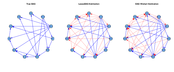
Figure 4: The estimated graphs compared with the human established graph. The blue edges are the correctly discovered ones and the red edges are false discoveries.

We also evaluate our model selection and covariance estimation procedures on the call center data used in [3] and [18]. The DAG Wishart model has better performance on that task as well. More details about this example can be found in the Supplemental section D subsection 4.4.

7 Closing Remarks

In this paper we undertake an in-depth analysis of the class of DAG-Wishart priors for Gaussian DAG models, with a view to developing a unified framework and tools for high dimensional Bayesian inference of these models. This work naturally extends the methodological results of Letac and Massam in [16] for decomposable graphs, and others in [14] for homogeneous graphs.

	DAG			UG			COVG
	ALL	P	H	ND	D	H	ND	D	H
Conjugacy
property	✔	✔	✔	✔	✔	✔	✗	✔	✔
Normalizing constant
in closed form	✔	✔	✔	✗	✔	✔	✗	✗	✔
Posterior moments
in closed from	✔	✔	✔	✗	✔	✔	✗	✗	✔
Posterior mode
in closed from	✔	✔	✔	✗	✔	✔	✗	✗	✔
Hyper Markov
properties	✔	✔	✔	✗	✔	✔	✗	✗	✔
Tractable sampling from
the distribution	✔	✔	✔	✗	✔	✔	✗	✔	✔

Table 3: Properties of Wishart distributions for the three classes of Gaussian graphical models. Abbreviations. ND: Non-decomposable, D/P: Decomposable/Perfect, H: Homogeneous.

Table 3 summarizes the properties of the various multi-parameter Wishart distributions that have been recently introduced to the statistics literature for use in Gaussian graphical models. One can see on this table that the DAG-Wishart distributions introduced in this paper are applicable in all generality - and not just when the graph is perfect, or equivalently, decomposable. The ability to specify the induced Wishart distributions and posterior moments for arbitrary graphs is especially useful.

Suplimental section A: Graph theory, Markov properties and Gaussian DAGs

Graph theoretic notation and terminology

A graph $\mathcal{G}$ is a pair of objects $(V,E)$, where $V$ and $E$ are two disjoint finite sets representing, respectively, the vertices and the edges of $\mathcal{G}$. Each edge in $E$ is either an ordered pair $(i,j)$ or an unordered pair $\{i,j\}$, for some $i,j\in V$. An edge $(i,j)\in E$ is called directed where $i$ is said to be a parent of $j$, and $j$ is said to be a child of $i$, when $i\neq j$. We write this as $i\rightarrow j$. The set of parents of $i$ is denoted by $\mathrm{pa}(i)$, and the set of children of $i$ is denoted by $\mathrm{ch}(i)$. The family of $i$ is $\mathrm{fa}(i)=\mathrm{pa}(i)\cup\{i\}$. An edge $\{i,j\}\in E$ is called undirected where $i$ is said to be a neighbor of $j$, or $j$ a neighbor of $i$, when $i\neq j$. We write this $i\sim_{\mathcal{G}}j$. The set of all neighbors of $i$ is denoted by $\mathrm{ne}(i)$. We say $i$ and $j$ are adjacent if there exists either a directed or an undirected edge between them. A loop in $\mathcal{G}$ is an ordered pair $(i,i)$, or an unordered pair $\{i,i\}$ in $E$. For ease of notation, in this paper we always shall assume that the edge set $E$ contains all the loops, although we shall draw the respective graphs without the loops.

We say that the graph $\mathcal{G}^{\prime}=(V^{\prime},E^{\prime})$ is a subgraph of $\mathcal{G}=(V,E)$, denoted by $\mathcal{G}^{\prime}\subset\mathcal{G}$, if $V^{\prime}\subset V$ and $E^{\prime}\subset E$. In addition, if $\mathcal{G}^{\prime}\subset\mathcal{G}$ and $E^{\prime}=V^{\prime}\times V^{\prime}\cap E$, we say that $\mathcal{G}^{\prime}$ is an induced subgraph of $\mathcal{G}$. We shall consider only induced subgraphs in what follows. For a subset $A\subset V$, the induced subgraph $\mathcal{G}_{A}=(A,A\times A\cap E)$ is said to be the graph induced by $A$. A graph $\mathcal{G}$ is called complete if every pair of vertices are adjacent. A clique of $\mathcal{G}$ is an induced complete subgraph of $\mathcal{G}$ that is not a subset of any other induced complete subgraphs of $\mathcal{G}$. More simply, a subset $A\subset V$ is called a clique if the induced subgraph $\mathcal{G}_{A}$ is a clique of $\mathcal{G}$. The set of the cliques of $\mathcal{G}$ is denoted by $\mathscr{C}_{\mathcal{G}}$.

A path in $\mathcal{G}$ of length $n\geq 1$ from a vertex $i$ to a vertex $j$ is a finite sequence of distinct vertices $i_{0}=i,\ldots,i_{n}=j$ in $V$ such that $(i_{\nu-1},i_{\nu})$ or $\{i_{\nu-1},\nu_{k}\}$ are in $E$ for each $\nu=1,\ldots,n$. We say that the path is directed if at least one of the edges is directed. We say $i$ leads to $j$, denoted by $i\longmapsto j$, if there is a directed path from $i$ to $j$. A graph $\mathcal{G}=(V,E)$ is called connected if for any pair of distinct vertices $i,j\in V$ there exists a path between them. An $n$-cycle in $\mathcal{G}$ is a path of length $n$ with the additional requirement that the end points are identical. A directed $n$-cycle is defined accordingly.

An undirected graph, which we denote by $\mathcal{G}=\left(V,\mathscr{E}\right)$, is a graph with all of its edges undirected. The undirected graph $\mathcal{G}$ is said to be decomposable if it has no induced cycle of length greater than or equal to four, excluding the loops. A constructive definition in terms of the cliques and the separators of the graph $\mathcal{G}$ can also be specified (The reader is referred to Lauritzen [15] for details.) A directed graph, denoted by $\mathcal{D}=\left(V,E\right)$, is now a graph with all of its edges directed. The directed graph $\mathcal{D}$ is said to be acyclic if it has no cycles, exlcuding the loops. The undirected version of a DAG $\mathcal{D}=(V,E)$, denoted by $\mathcal{D}^{u}=\left(V,E^{u}\right)$, is the undirected graph obtained by replacing all the directed edges of $\mathcal{D}$ by undirected ones. An immorality in a directed graph $\mathcal{D}$ is an induced subgraph of the from $i\rightarrow k\leftarrow j$. Moralizing an immorality entails adding an undirected edge between the pair of parents that have the same children. Then the moral graph of $\mathcal{D}$, denoted by $\mathcal{D}^{p}=\left(V,E^{p}\right)$, is the undirected graph obtained by first moralizing each immorality of $\mathcal{D}$ and then making the undirected version of the resulting graph. A DAG $\mathcal{D}$ is said to be perfect if it has no immoralities; i.e., the parents of all vertices are adjacent, or equivalently if the set of parents of each vertex induces a complete subgraph of $\mathcal{D}$. Decomposable (undirected) graphs and (directed) perfect graphs have a deep connection. In particular, it can be shown [15] that if $\mathcal{G}$ is decomposable, then there exists a DAG version of $\mathcal{G}$, i.e., a DAG $\mathcal{D}$ such that $\mathcal{D}^{u}=\mathcal{G}$, where $\mathcal{D}$ is a perfect DAG.

Given a DAG, the set of ancestors of a vertex $j$, denoted by $\mathrm{an}(j)$, is the set of those vertices $i$ such that $i\longmapsto j$. Similarly, the set of descendants of a vertex $i$, denoted by $\mathrm{de}(i)$, is the set of those vertices $j$ such that $i\longmapsto j$. The set of non-descendants of $i$ is $\mathrm{nd}(i)=V\setminus\left(\mathrm{de}(i)\cup\{i\}\right)$. A set $A\subseteq V$ is called ancestral when $A$ contains the parents of its members. The smallest ancestral set containing the subset $B$ of $V$ is denoted by $\mathrm{An}(B)$.

Markov properties for DAG models

Let $V$ be a finite set of indices and $(X_{i})_{i\in V}$ a collection of random variables, where each $X_{i}$ is a random variable on the probability space $\mathcal{X}_{i}$. Let the probability space $\mathcal{X}$ be defined as the product space $\mathcal{X}=\times_{i\in V}\mathcal{X}_{i}$. Now let $\mathcal{D}=(V,E)$ be a DAG. For simplicity, and without loss of generality, we always assume that the given DAG $\mathcal{D}$ is connected and the edge set $E$ contains all the loops $(i,i),i\in V$. We say that a probability distribution $P$ on $\mathcal{X}$ has the recursive factorization property w.r.t. $\mathcal{D}$, denoted by DF (the directed factorization property), if there are $\sigma$-finite measures $\mu_{i}$ on $\mathcal{X}_{i}$ and non-negative functions $k^{i}(x_{i},x_{pa(i)})$, referred to as kernels, defined on $\mathcal{X}_{fa(i)}$ such that

$$\int k^{i}(y_{i},x_{pa(i)})d\mu_{i}(y_{i})=1,\quad\forall i\in V,$$

and $P$ has a density $p$, w.r.t. the product measure $\mu=\otimes_{i\in V}\mu_{i}$, given by

$$p(x)=\prod_{i\in V}k^{i}(x_{i},x_{pa(i)}).$$

In this case, each kernel $k^{i}(x_{i},x_{pa(i)})$ is in fact a version of $p(x_{i}|x_{pa(i)})$, the conditional distribution of $X_{i}$ given $X_{pa(i)}$. An immediate consequence of this definition is the following lemma.

Lemma 7.1.

[15] If $P$ admits a recursive factorization w.r.t. the directed graph $\mathcal{D}$, then it also admits a factorization w.r.t. the undirected graph $\mathcal{D}^{\mathrm{m}}$, and, consequently, obeys the global Markov property w.r.t. $\mathcal{D}^{\mathrm{m}}$.

Proof.

Note that for each vertex $i\in V$ the set $fa(i)$ is a complete subset of $\mathcal{D}^{\mathrm{m}}$. Thus if we define $\psi_{fa(i)}(x_{fa(i)})=k^{i}(x_{i},x_{pa(i)})$, then $p(x)=\prod_{i\in V}p(x_{i}|x_{pa(i)})=\prod_{i\in V}k^{i}(x_{i},x_{pa(i)})=\prod_{i\in V}\psi_{fa(i)}(x_{fa(i)})$. Therefore, $P$ admits a factorization w.r.t. $\mathcal{D}^{\mathrm{m}}$ and by proposition 3.8 in [15] it also obeys the global Markov property w.r.t. $\mathcal{D}^{\mathrm{m}}$. ∎

Another direct implication of the DF property is that if $P$ admits a recursive factorization w.r.t. $\mathcal{D}$, then, for each ancestral set $A$, the marginal distribution $P_{A}$ admits a recursive factorization w.r.t. the induced graph $\mathcal{D}_{A}$. Combining this result with Lemma 7.1 we obtain the following: P admits a recursive factorization w.r.t. $\mathcal{D}$ then $A\perp\!\!\!\perp B|S\ [P]$, whenever $A$ and $B$ are separated by $S$ in $(\mathcal{D}_{An(A\cup B\cup S)})^{\mathrm{m}}$. We call this property the directed global Markov property, DG, and any distribution that satisfies this property is said to be a directed Markov field over $\mathcal{D}$. For DAGs the directed Markov property plays the same role as the global Markov property does for undirected graphs, in the sense that it provides an optimal rule for recovering the conditional independence relations encoded by the directed graph.

We now introduce below another Markov property for DAGs. A distribution $P$ on $\mathcal{X}$ is said to obey the directed local Markov property (DL) w.r.t. $\mathcal{D}$ if for each $i\in V$

$$i\perp\!\!\!\perp nd(i)|pa(i).$$

Now for a given DAG $\mathcal{D}$ consider the so-called “parent graph” defined as follows: The parent graph $\mathcal{D}_{par}$ of $\mathcal{D}$ is a DAG isomorphic to $\mathcal{D}$ and obtained by relabeling the vertex set $V$ as $1,2,\ldots,|V|,$ in such a way that $pa(i)\subseteq\left\{i+1,\ldots,|V|\right\}$ for each vertex $i\in V$. It is easily shown that for any given DAG it is possible to relabel the vertices so that parents always have a higher numbering that their respective children though such an ordering is not unique in general. For a given parent ordering we say that $P$ obeys the parent ordered Markov property (PO) w.r.t. $\mathcal{D}$ if for every vertex $i$ we have

$$i\perp\!\!\!\perp\left\{i+1,\ldots,|V|\right\}\setminus pa(i)|pa(i).$$

It can be shown that if $P$ has a density w.r.t. $\mu$, then $P$ obeys one of the directed Markov properties DF, DG, DL, PO iff it obeys all of them, i.e., the four Markov properties for DAGs are equivalent under mild conditions [15].

Linear recursive properties of Gaussian DAGs

Let $\mathbf{x}=\left(x_{1},\ldots,x_{p}\right)^{\top}$ be a random vector in $\mathbb{R}^{p}$ with the multivariate distribution $\rm{N}_{p}(0,\Sigma)$. Consider the system of linear recursive regression equations:

where $-\beta_{ij}$ is the partial regression coefficient of $x_{j}$ ($j>i$) in the regression of $x_{i}$ on its predecessors $x_{i+1},\ldots,x_{j},\ldots,x_{p}$. Now $\beta_{ij}$ is zero iff $i\perp\!\!\!\perp\left\{i+1,\ldots,|V|\right\}\setminus pa(i)\;|\;pa(i)$ . Hence the partial regression coefficient $\beta_{ij}$ is zero if there does not exist an arrow from $j$ to $i$, i.e., $j\notin pa(i)$, $j>i$. In addition, the residuals $\epsilon_{i}$ are normally distributed and mutually independent with mean zero and variance $\sigma^{2}_{ii|pa(i)}$. We can rewrite the first system of equations in the form of a linear system $B\mathbf{x}=\boldsymbol{\epsilon}$, where $B$ is the upper triangular matrix

$$B=\left(\begin{matrix}1&\beta_{12}&\ldots&\beta_{1p}\\ 0&1&\ldots&\beta_{2p}\\ 0&\ldots&\ddots&\vdots\\ 0&\ldots&0&1\\ \end{matrix}\right),\quad\mathbf{x}=\left(\begin{matrix}x_{1}\\ x_{2}\\ \vdots\\ x_{p}\end{matrix}\right)\quad\text{and}\quad\boldsymbol{\epsilon}=\left(\begin{matrix}\epsilon_{1}\\ \epsilon_{2}\\ \vdots\\ \epsilon_{p}\end{matrix}\right).$$

From this we obtain:

$$\mathbb{V}ar[B\mathbf{x}]=\mathbb{V}ar[\mathbf{\epsilon}]$$

$$\Rightarrow B\Sigma B^{\top}=diag(\sigma^{2}_{1|pa(1)},\ldots,\sigma^{2}_{p-1|pa(p-1)},\sigma^{2}_{pp})=:D$$

$$\Rightarrow \Sigma=B^{-1}D(B^{\top})^{-1}$$

$$\Rightarrow \Sigma^{-1}=B^{\top}D^{-1}B.$$ (20)

Thus, if we define $L=B^{\top}$, then $\Sigma^{-1}=LD^{-1}L^{\top}$ is the modified Cholesky decomposition of $\Sigma^{-1}$, in terms of the lower triangular matrix $L$ and the diagonal matrix $D^{-1}$. Now consider a DAG denoted by $\mathcal{D}=(V,E)$. In [23] it has been shown that $\rm{N}_{p}(0,\Sigma)$ obeys the directed Markov property w.r.t. $\mathcal{D}$ iff $L_{ij}=0$ whenever there is no arrow from $i$ to $j$, i.e., $i\notin pa(j)$. (20) above therefore gives a very convenient description of the Gaussian DAG model $\mathscr{N}(\mathcal{D})$. We explore this model in more detail below.

Supplemental Section B: Properties of the class of DAG-Wishart distributions

7.1 Deriving the closed form expression for the DAG-Wishart $\pi_{U,\alpha}^{\Theta_{\mathcal{D}}}$

Theorem 7.2.

Let $dL:=\prod_{(i,j)\in E,i>j}dL_{ij}$ and $dD:=\prod_{i=1}^{p}dD_{ii}$ denote, respectively, the canonical Lebesgue measures on $\mathcal{L}_{\mathcal{D}}$ and $\mathbb{R}^{p}_{+}$ and let $pa_{i}:=|pa(i)|$. Then,

$$\int_{\Uptheta_{\mathcal{D}}}\exp\{-\frac{1}{2}\mathrm{tr}(LD^{-1}L^{t}U)\}\prod_{i=1}^{p}D^{-\frac{1}{2}\alpha_{i}}_{ii}dLdD<\infty$$

if and only if

$$\alpha_{i}>pa_{i}+2\;\;\;\forall i=1,\ldots,p.$$

Furthermore, in this case

$$z_{\mathcal{D}}(U,\alpha)=\prod_{i=1}^{p}\frac{\Gamma\left(\frac{\alpha_{i}}{2}-\frac{pa_{i}}{2}-1\right)2^{\frac{\alpha_{i}}{2}-1}(\sqrt{\pi})^{pa_{i}}\det(U_{\prec i\succ})^{\frac{\alpha_{i}}{2}-\frac{pa_{i}}{2}-\frac{3}{2}}}{\det(U_{\preceq i\succeq})^{\frac{\alpha_{i}}{2}-\frac{pa_{i}}{2}-1}}.$$ (21)

Proof.

Let us first simplify the expression by integrating out the terms involving $D_{ii}$’s.

$$\int\exp\left\{-\frac{1}{2}\mathrm{tr}\left(\left(LD^{-1}L^{\top}\right)U\right)\right\}\prod^{p}_{i=1}D_{ii}^{-\frac{1}{2}\alpha_{i}}dLdD$$

$$= \int\exp\left\{-\frac{1}{2}\mathrm{tr}\left(D^{-1}\left(L^{\top}UL\right)\right)\right\}\prod_{i=1}^{p}D^{-\frac{1}{2}\alpha_{i}}_{ii}dLdD$$

$$= \int\exp\left\{-\frac{1}{2}\sum^{p}_{i=1}D^{-1}_{ii}(L^{\top}UL)_{ii}\right\}\prod^{p}_{i=1}D_{ii}^{-\frac{1}{2}\alpha_{i}}dDdL$$

$$= \int\left(\prod_{i=1}^{p}\int\exp\left\{-\frac{1}{2}D^{-1}_{ii}(L^{\top}UL)_{ii}\right\}D_{ii}^{-\frac{1}{2}\alpha_{i}}dD_{ii}\right)dL$$

$$= \int\prod_{i=1}^{p}\frac{\Gamma\left(\frac{\alpha_{i}}{2}-1\right)2^{\frac{\alpha_{i}}{2}-1}}{\left(\left(L^{\top}UL\right)_{ii}\right)^{\frac{\alpha_{i}}{2}-1}}dL\qquad(\text{ iff }\alpha_{i}>2\;\forall\;i=1,2,\cdots,p)$$

$$= \int\prod_{i=1}^{p}\frac{\Gamma\left(\frac{\alpha_{i}}{2}-1\right)2^{\frac{\alpha_{i}}{2}-1}}{\left((L_{\cdot i})^{\top}UL_{\cdot i}\right)^{\frac{\alpha_{i}}{2}-1}}dL$$

$$= \int\prod_{i=1}^{p}\frac{\Gamma\left(\frac{\alpha_{i}}{2}-1\right)2^{\frac{\alpha_{i}}{2}-1}}{\left(\left(\begin{matrix}1&L^{\top}_{\prec i]}\end{matrix}\right)\left(\begin{matrix}U_{ii}&U_{[i\succ}\\ U_{\prec i]}&U_{\prec i\succ}\end{matrix}\right)\left(\begin{matrix}1\\ L_{\prec i]}\end{matrix}\right)\right)^{\frac{\alpha_{i}}{2}-1}}dL$$

$$= \prod_{i=1}^{p}\int_{\mathbb{R}^{pa_{i}}}\frac{\Gamma\left(\frac{\alpha_{i}}{2}-1\right)2^{\frac{\alpha_{i}}{2}-1}}{\left(\left(\begin{matrix}1&L^{\top}_{\prec i]}\end{matrix}\right)\left(\begin{matrix}U_{ii}&U_{[i\succ}\\ U_{\prec i]}&U_{\prec i\succ}\end{matrix}\right)\left(\begin{matrix}1\\ L_{\prec i]}\end{matrix}\right)\right)^{\frac{\alpha_{i}}{2}-1}}dL_{\prec i]}.\qquad\text{eqn(A)}$$

We now show how in general one can evaluate an integral of the form

$$\int_{\mathbb{R}^{d}}\frac{d\mathbf{x}}{\left(\left(\begin{matrix}1&\mathbf{x}^{\top}\end{matrix}\right)\left(\begin{matrix}a&\mathbf{b}^{\top}\\ \mathbf{b}&A\end{matrix}\right)\left(\begin{matrix}1\\ \mathbf{x}\end{matrix}\right)\right)^{\gamma}},$$

where the block partitioned matrices, formed by $a\in\mathbb{R}$, $\mathbf{b}\in\mathbb{R}^{d}$ and the $(d-1)\times(d-1)$ matrix $A$, is positive definite. In order to simplify the above integral we proceed in two steps.

$1)$ We first note that by the formula provided on [6, page 16] that,

$$\int_{\mathbb{R}}\frac{1}{(1+x^{2})^{\gamma}}dx=\begin{cases}\frac{\sqrt{\pi}\Gamma\left(\gamma-\frac{1}{2}\right)}{\Gamma(\gamma)}&\gamma>\frac{1}{2},\cr\infty&\mbox{otherwise}.\end{cases}$$

By repeated application, we can generalize the above formula to

$$\int_{\mathbb{R}^{d}}\frac{1}{({\bf x}^{\top}{\bf x}+1)^{\gamma}}d{\bf x}=\begin{cases}\frac{(\sqrt{\pi})^{d}\Gamma\left(\gamma-\frac{d}{2}\right)}{\Gamma(\gamma)}&\gamma>\frac{d}{2},\cr\infty&\mbox{otherwise}.\end{cases}$$

$2)$  Let us now consider the general integral

$$\int_{\mathbb{R}^{d}}\displaystyle\frac{d\mathbf{x}}{\left(\left(\begin{matrix}1&\mathbf{x}^{\top}\end{matrix}\right)\left(\begin{matrix}a&\mathbf{b}^{\top}\\ \mathbf{b}&A\end{matrix}\right)\left(\begin{matrix}1\\ \mathbf{x}\end{matrix}\right)\right)^{\gamma}}.$$

Making the linear transformation ${\bf y}=A^{\frac{1}{2}}{\bf x}+A^{-\frac{1}{2}}\mathbf{b}$ it follows that for $\gamma>\frac{d}{2}$,

$$\int_{\mathbb{R}^{d}}\displaystyle\frac{d\mathbf{x}}{\left(\left(\begin{matrix}1&\mathbf{x}^{\top}\end{matrix}\right)\left(\begin{matrix}a&\mathbf{b}^{\top}\\ \mathbf{b}&A\end{matrix}\right)\left(\begin{matrix}1\\ \mathbf{x}\end{matrix}\right)\right)^{\gamma}} = \frac{1}{\det(A)^{\frac{1}{2}}}\int_{\mathbb{R}^{d}}\displaystyle\frac{1}{\left({\bf y}^{\top}{\bf y}+a-\mathbf{b}^{\top}A^{-1}\mathbf{b}\right)^{\gamma}}d{\bf y}$$ (22)

$$= \displaystyle\frac{(\sqrt{\pi})^{d}\Gamma\left(\gamma-\frac{d}{2}\right)}{\Gamma(\gamma)\det(A)^{\frac{1}{2}}\left(a-\mathbf{b}^{\top}A^{-1}\mathbf{b}\right)^{\gamma-\frac{d}{2}}}.$$

Applying the result from (22) to the desired integral in (A) we obtain

$$z_{\mathcal{D}}(U,{\bf\alpha}) = \prod_{i=1}^{p}\int_{\mathbb{R}^{pa_{i}}}\frac{\Gamma\left(\frac{\alpha_{i}}{2}-1\right)2^{\frac{\alpha_{i}}{2}-1}}{\left(\left(\begin{matrix}1&L^{\top}_{\prec i]}\end{matrix}\right)\left(\begin{matrix}U_{ii}U_{[i\succ}\\ U_{\prec i]}&U_{\prec i\succ}\end{matrix}\right)\left(\begin{matrix}1\\ L_{\prec i]}\end{matrix}\right)\right)^{\frac{\alpha_{i}}{2}-1}}dL_{\prec i]}$$

$$= \prod_{i=1}^{p}\frac{\Gamma\left(\frac{\alpha_{i}}{2}-\frac{pa_{i}}{2}-1\right)2^{\frac{\alpha_{i}}{2}-1}(\sqrt{\pi})^{pa_{i}}\det(U_{\prec i\succ})^{\frac{\alpha_{i}}{2}-\frac{pa_{i}}{2}-\frac{3}{2}}}{\det(U_{\preceq i\succeq})^{\frac{\alpha_{i}}{2}-\frac{pa_{i}}{2}-1}},$$

where $\det(U_{\prec i\succ})=1$ whenever $pa(i)=\emptyset$. It is easily seen that $z_{\mathcal{D}}(U,{\bf\alpha})$ is finite iff $\alpha_{i}>pa_{i}+2$ for each $i=1,\ldots,p.$ ∎

The Hyper Morkov properties of the DAG-Wishart

Theorem 7.3.

Let $\mathcal{D}$ be an arbitrary DAG and $(D,L)\sim\pi^{\Theta_{\mathcal{D}}}_{U,{\bf\alpha}}$.Then $\{(D_{ii},L_{\prec i]}):i=1,\ldots,p\}$ are mutually independent. Moreover,

$$D_{ii}\sim IG(\frac{\alpha_{i}}{2}-\frac{pa_{i}}{2}-1,\frac{1}{2}U_{ii|\prec i\succ}),~{}\text{and}$$ (23)

$$L_{\prec i]}|D_{ii}\sim\mathrm{N}_{pa_{i}}(-U^{-1}_{\prec i\succ}U_{\prec i]},D_{ii}U^{-1}_{\prec i\succ}).$$ (24)

Proof.

First consider the bijective mapping from the Cholesky parametrization to the D-parametrization:

$$\phi=\left((D,L)\mapsto\times_{i\in V}(D_{ii},L_{\prec i]})\right):\Theta_{\mathcal{D}}\rightarrow\Xi_{\mathcal{D}},$$ (25)

with the inverse mapping $\left(\times_{i\in V}(\lambda_{i},\beta_{\prec i]})\mapsto(D,L)\right):\Xi_{\mathcal{D}}\rightarrow\Theta_{\mathcal{D}}$, where $D=\mathrm{diag}(\lambda_{1}\ldots,\lambda_{p})$ and

$$L_{ij}=\begin{cases}1&i=j\\ L_{ij}=\beta_{ij}&i\in pa(j)\\ 0&\text{otherwise}\end{cases}$$

Since $\beta_{\prec j]}=(\beta_{ij}:i\in pa(j))$ belongs to $\mathbb{R}^{\prec j]}$, the mapping $\pi_{U,\alpha}^{\Theta_{\mathcal{D}}}$ naturally induces a prior on $\Xi_{\mathcal{D}}$ which we shall denote by $\pi^{\Xi_{\mathcal{D}}}_{U,{\bf\alpha}}$. Note that the D and Cholesky parametrizations of a Gaussian DAG model $\mathscr{N}(\mathcal{D})$ are essentially the same, since they both encode the partial regression coefficients and partial variances in the corresponding system of recursive regression equations (as described in Supplemental Section A). Hence the Jacobian of $\phi$ is equal to $1$. To derive the density of $\pi^{\Xi_{\mathcal{D}}}_{U,{\bf\alpha}}$ it suffices to find an expression for $\mathrm{tr}((LD^{-1}L^{\top})U)$ in terms of $\prod_{i\in V}(D_{ii},L_{\prec i]})$. To this end, we proceed as follows.

$$\mathrm{tr}((LD^{-1}L^{\top})U)=\mathrm{tr}(D^{-1}L^{\top})UL)=\sum_{i\in V}D^{-1}_{ii}(L^{\top}UL)_{ii}$$

$$=\sum_{i\in V}D^{-1}_{ii}(\sum_{k,l\in V}L_{ki}U_{kl}L_{li})$$

$$=\sum_{i\in V}D^{-1}_{ii}\left(\begin{matrix}1\\ L_{\prec i]}\end{matrix}\right)^{\top}\left(\begin{matrix}U_{ii}&U_{[i\succ}\\ U_{\prec i]}&U_{\prec i\succ}\end{matrix}\right)\left(\begin{matrix}1\\ L_{\prec i]}\end{matrix}\right)$$

$$=\sum_{i\in V}D^{-1}_{ii}(U_{ii}+L_{\prec i]}^{\top}U_{\prec i]}+U_{[i\succ}L_{\prec i]}+L^{\top}_{\prec i]}U_{\prec i\succ}L_{\prec i]})$$

$$=\sum_{i\in V}\left(D^{-1}_{ii}(L_{\prec i]}+U^{-1}_{\prec i\succ}U_{\prec i]})^{\top}U_{\prec i\succ}(L_{\prec i]}+U^{-1}_{\prec i\succ}U_{\prec i]})+D^{-1}_{ii}U_{ii|\prec i\succ}\right).$$

Therefore, the density of $\pi^{\Xi_{\mathcal{D}}}_{U,{\bf\alpha}}$ w.r.t. the Lebesgue measure $\prod_{i\in V}d\lambda_{i}d\beta_{\prec i]}$ on $\times_{i\in V}(\mathbb{R}_{+},\mathbb{R}^{\prec i]})$ is given by

$$z_{\mathcal{D}}(\alpha,U)^{-1}\exp\left\{-\frac{1}{2}\sum_{i\in V}\left(\lambda^{-1}_{i}(\beta_{\prec i]}+U^{-1}_{\prec i\succ}U_{\prec i]})^{\top}U_{\prec i\succ}(\beta_{\prec i]}+U^{-1}_{\prec i\succ}U_{\prec i]})+\lambda^{-1}_{i}U_{ii|\prec i\succ}\right)\right\}\prod_{i\in V}\lambda^{-\frac{1}{2}\alpha_{i}}_{i}.$$ (26)

The above clearly shows that $\left\{(\lambda_{i},\beta_{\prec i]}):i=1,\ldots,p\right\}$ are mutually independent. To complete the proof we first integrate out $\beta_{\prec i]}$ to obtain the marginal density of $\lambda_{i}$. Notice that the expression involving $\beta_{\prec i]}$ in (26) is an unrealized multivariate normal integral and thus (26) can be expressed as follows:

$$\int_{\mathbb{R}^{\prec i]}}\exp\left\{-\frac{1}{2}\sum_{i\in V}\lambda_{i}^{-1}(\beta_{\prec i]}+U^{-1}_{\prec i\succ}U_{\prec i]})^{\top}U_{\prec i\succ}(\beta_{\prec i]}-U^{-1}_{\prec i\succ}U_{\prec i]})+\lambda_{i}^{-1}U_{ii|\prec i\succ}\right\}\prod_{i\in V}\lambda_{i}^{-\frac{1}{2}\alpha_{i}}d(\beta_{\prec i]})$$ (27)

$$\propto\exp\left\{-\frac{1}{2}\lambda^{-1}_{i}U_{ii|\prec i\succ}\right\}\prod_{i\in V}\lambda^{-\frac{1}{2}\alpha_{i}+\frac{1}{2}pa_{i}}_{i}$$

The above shows that $\lambda_{i}\sim IG(\alpha_{i}/2-pa_{i}/2-1,U_{ii|\prec i\succ}/2)$. It is evident from (27) that $\beta_{\prec i]}|\lambda_{i}\sim\rm{N}_{pa_{i}}(-U^{-1}_{\prec i\succ}U_{\prec i]},\lambda_{i}U^{-1}_{\prec i\succ})$. It is also immediately clear that the same result holds for elements of the Cholesky-parametrization $(D_{ii},L_{\prec i]}),\;i=1,2,\ldots,p$ as specified in the statement of the theorem. ∎

The converse part of Theorem 7.3 is obvious and left to the reader.

Corollary 5.

Let $\mathcal{D}$ be an arbitrary DAG and suppose $(L,D)\sim\pi^{\Theta_{\mathcal{D}}}_{U,\alpha}$. Then the density of $L$ w.r.t. $dL=\prod_{i=1}^{p}dL_{\prec i]}$ is given by

$$\prod_{i=1}^{p}c_{i}\left[1/2U_{ii|\prec i\succ}+(L_{\prec i]}+U_{\prec i\succ}^{-1}U_{\prec i]})^{t}U_{\prec i\succ}(L_{\prec i]}+U_{\prec i\succ}^{-1}U_{\prec i]})\right]^{-\alpha_{i}/2+1},$$

where each $c_{i}$ is given by

$$\frac{\det(U_{\prec i\succ})^{1/2}(U_{ii|\prec i\succ})^{\alpha_{i}/2-pa_{i}/2-1}\Gamma(\alpha_{i}/2-1)}{2^{\alpha_{i}/2-1}\pi^{pa_{i}/2}\Gamma(\alpha_{i}/2-pa_{i}/2-1)}.$$ (28)

Proof.

Using Theorem 7.3 we compute:

$$\int\displaystyle\frac{1}{(2\pi)^{pa_{i}/2}\det(D_{ii}U_{\prec i\succ}^{-1})^{1/2}}\exp\left\{(L_{\prec i]}+U_{\prec i\succ}^{-1}U_{\prec i]})^{\top}(D_{ii}^{-1}U_{\prec i\succ})(L_{\prec i]}+U_{\prec i\succ}^{-1}U_{\prec i]})\right\}$$

$$\times\displaystyle\frac{(1/2U_{ii|\prec i\succ})^{\alpha_{i}/2-pa_{i}/2-1}}{\Gamma(\alpha_{i}/2-pa_{i}/2-1)}D_{ii}^{-\alpha_{i}/2+pa_{i}/2}\exp\left\{-1/2U_{ii|\prec i\succ}D_{ii}^{-1}\right\}dD_{ii}$$

$$= \displaystyle\frac{\det(U_{\prec i\succ})^{1/2}(U_{ii|\prec i\succ})^{\alpha_{i}/2-pa_{i}/2-1}}{2^{\alpha_{i}/2-1}\pi^{pa_{i}/2}\Gamma(\alpha_{i}/2-pa_{i}/2-1)}\int D_{ii}^{-\alpha_{i}/2}\exp\left\{-u_{i}D_{ii}^{-1}\right\}dD_{ii}$$

$$= \displaystyle\frac{\det(U_{\prec i\succ})^{1/2}(U_{ii|\prec i\succ})^{\alpha_{i}/2-pa_{i}/2-1}}{2^{\alpha_{i}/2-1}\pi^{pa_{i}/2}\Gamma(\alpha_{i}/2-pa_{i}/2-1)}\times\displaystyle\frac{\Gamma(\alpha_{i}/2-1)}{u_{i}^{\alpha_{i}/2-1}},$$

where $u_{i}=1/2U_{ii|\prec i\succ}+(L_{\prec i]}+U_{\prec i\succ}^{-1}U_{\prec i]})^{\top}U_{\prec i\succ}(L_{\prec i]}+U_{\prec i\succ}^{-1}U_{\prec i]}).$ Therefore the density of $L_{\prec i]}$ is given by

$$c_{i}\left(1/2U_{ii|\prec i\succ}+(L_{\prec i]}+U_{\prec i\succ}^{-1}U_{\prec i]})^{\top}U_{\prec i\succ}(L_{\prec i]}+U_{\prec i\succ}^{-1}U_{\prec i]})\right)^{-\alpha_{i}/2+1}.$$ (29)

By Theorem 7.3 $L_{\prec i]}$ are mutually independent, hence the form of the density in the statement of the corollary is immediate from the above calculations. The parameters corresponding to the t-distribution follow by comparing the density in (29) to the functional form of the density of the multivariate t-distribution. ∎

The Posterior distribution of the DAG-Wishart

Proposition 7.4.

Let $\mathcal{D}$ be an arbitrary DAG and let ${\bf Y}_{1},{\bf Y}_{2},\cdots,{\bf Y}_{n}$ be an i.i.d. sample from $\rm{N}_{p}({\bf 0},(L^{-1})^{\top}DL^{-1})$, where $(D,L)\in\Theta_{\mathcal{D}}$. Let $S=\frac{1}{n}\sum_{i=1}^{n}{\bf Y}_{i}{\bf Y}_{i}^{\top}$ denote the empirical covariance matrix. If the prior distribution on $(D,L)$ is $\pi_{U,\alpha}^{\Theta_{\mathcal{D}}}$, then the posterior distribution of $(D,L)$ is given by $\pi_{\widetilde{U},\widetilde{\bf\alpha}}^{\Theta_{\mathcal{D}}}$, where $\widetilde{U}=nS+U$ and $\widetilde{\bf\alpha}=(n+\alpha_{1},n+\alpha_{2},\cdots,n+\alpha_{p})$.

Proof.

The likelihood of the data is given as follows:

$$f({\bf y}_{1},{\bf y}_{2},\cdots,{\bf y}_{n}\mid L,D)=\frac{1}{(\sqrt{2\pi})^{np}}\exp\left\{-\frac{1}{2}\mathrm{tr}\left(LD^{-1}L^{\top}(nS)\right)\right\}\det(D)^{-\frac{1}{2}n}.$$

When using $\pi_{U,\alpha}^{\Theta_{\mathcal{D}}}$ as the prior for $(D,L)$, the posterior distribution of $(D,L)$ given the data $({\bf Y}_{1},{\bf Y}_{2},\cdots,{\bf Y}_{n})$ is given by

$$\pi_{U,\alpha}^{\Theta_{\mathcal{D}}}(L,D\mid{\bf Y}_{1},{\bf Y}_{2},\cdots,{\bf Y}_{n})\propto\exp\left\{-\frac{1}{2}\mathrm{tr}\left(LD^{-1}L^{\top}(nS+U)\right)\right\}\prod_{i=1}^{p}D^{-\frac{n+\alpha_{i}}{2}}_{ii},\;\;(D,L)\in\Theta_{\mathcal{D}}.$$ (30)

Hence the functional form of the posterior density is the same as that of the prior density, i.e.,

$$\pi_{U,\alpha}^{\Theta_{\mathcal{D}}}(\cdot\mid{\bf Y}_{1},{\bf Y}_{2},\cdots,{\bf Y}_{n})=\pi_{\widetilde{U},\widetilde{\bf\alpha}}(\cdot),$$

where $\widetilde{U}=nS+U$ and $\widetilde{\alpha}=(\alpha_{1}+n,\ldots,\alpha_{p}+n)$. ∎

Remark 7.1.

The case when the observations do not have mean zero (i.e., when ${\bf Y}_{1},{\bf Y}_{2},\cdots,{\bf Y}_{n}$ are i.i.d. $\rm{N}_{p}({\bf\mu},\Sigma)$, with ${\bf\mu}\in\mathbb{R}^{p},\;\Sigma\in\mathrm{PD}_{\mathcal{D}}$) can be handled in a similar manner by noting that the sample covariance matrix $S$ is a sufficient statistic for $\Sigma$ and the fact that $nS\sim\mathrm{W}_{p}(n-1,\Sigma)$.

The Laplace transform of the DAG-Wishart

We start with computing the Laplace transform of $\pi^{\Xi_{\mathcal{D}}}_{U,\alpha}$ by exploiting the results established in Theorem 7.3. First a preliminary result on the Laplace transform of a Gaussian inverse Gamma distribution is required.

Lemma 7.5.

Suppose $(\lambda,\mathbf{x})$ is a random variable with Gaussian-inverse gamma distribution:

$$\mathbf{x}|\lambda \sim\mathrm{N}_{p}(\mu,\lambda\Psi),\quad\mu\in\mathbb{R}^{p},\Psi\in\mathrm{PD}_{p}(\mathbb{R});$$

$$\lambda \sim\mathrm{IG}(\nu,\eta).$$

Then the Laplace transform of $(\lambda,\mathbf{x})$ at $(\xi,u)\in\mathbb{R}_{+}\times\mathbb{R}_{+}^{p}$ is

$$\frac{2}{\Gamma(\nu)}\exp\{u^{\top}\mu\}\left(\eta(\xi-\frac{1}{2}u^{\top}\Psi u)\right)^{\frac{1}{2}\nu}K_{\nu}\left(2\sqrt{\eta(\xi-\frac{1}{2}u^{\top}\Psi u)}\right),$$

where $K_{\nu}(\cdot)$ is the modified Bessel function of the second type and $\xi-\frac{1}{2}u^{\top}\Psi u$ is assumed to be positive.

Proof.

By definition, the Laplace transform of $(\lambda,\mathbf{x})$ at $(\xi,u)\in\mathbb{R}\times\mathbb{R}^{p}$ is

$$\int\exp\{-(\lambda\xi+u^{\top}x)\}d\mathrm{N}_{p}(\mu,\lambda\Psi)(x)d\mathrm{IG}(\nu,\eta)(\lambda)$$

$$= \int\exp\{-\lambda\xi\}\left(\int\exp\{-u^{\top}x)\}d\mathrm{N}_{p}(\mu,\lambda\Psi)(x)\right)d\mathrm{IG}(\nu,\eta)(\lambda)$$

$$= \int\exp\{-\lambda\xi\}\exp\{-u^{\top}\mu+\frac{1}{2}\lambda u^{\top}\Psi u\}d\mathrm{IG}(\nu,\eta)(\lambda)$$

$$= \int\exp\{-\lambda\xi\}\exp\{-u^{\top}\mu+\frac{1}{2}\lambda u^{\top}\Psi u\}\left(\frac{\eta^{\nu}}{\Gamma(\nu)}\exp\{-\eta\lambda^{-1}\}\lambda^{-\nu-1}\right)d\lambda$$

$$= \frac{\eta^{\nu}}{\Gamma(\nu)}\exp\{-u^{\top}\mu\}\int\exp\{-(\xi-\frac{1}{2}u^{\top}\Psi u)\lambda-\eta\lambda^{-1}\}\lambda^{-\nu-1}d\lambda$$

$$= \frac{2\eta^{\nu}}{\Gamma(\nu)}\exp\{-u^{\top}\mu\}\left(\frac{\xi-\frac{1}{2}u^{\top}\Psi u}{\eta}\right)^{\frac{1}{2}\nu}K_{\nu}\left(2\sqrt{\eta(\xi-\frac{1}{2}u^{\top}\Psi u)}\right)$$

$$= \frac{2}{\Gamma(\nu)}\exp\{-u^{\top}\mu\}\left(\eta(\xi-\frac{1}{2}u^{\top}\Psi u)\right)^{\frac{1}{2}\nu}K_{\nu}\left(2\sqrt{\eta(\xi-\frac{1}{2}u^{\top}\Psi u)}\right).$$

Note that in computing the integral above we have used the fact that the Laplace transform of $\mathrm{N}_{p}(\mu,\lambda\Psi)$ at $u$ is equal to $\exp\{-u^{\top}\mu+\frac{1}{2}\lambda u^{\top}\Psi u\}$. For computing the integral w.r.t. $d\lambda$ we use the Equation (9.42) in [22, page 235].

∎

Proposition 7.6.

The Laplace transform of $\pi^{\Xi_{\mathcal{D}}}_{U,\alpha}$ at a typical point $\times_{i=1}^{p}(\xi_{i},z_{\prec i]})\in\Xi_{\mathcal{D}}$ is given by

$$\mathcal{L}_{\Xi_{\mathcal{D}}}(\times_{i=1}^{p}(\xi_{i},z_{\prec i]})):=2^{p}\prod_{i=1}^{p}\frac{1}{\Gamma(r_{i})}\exp\{z_{\prec i]}^{\top}\mu_{\prec i]}\}\left(\eta_{i}(\xi_{i}-\frac{1}{2}z_{\prec i]}^{\top}\Psi_{\prec i\succ}z_{\prec i]})\right)^{\frac{1}{2}r_{i}}$$ (31)

$$\times K_{r_{i}}\left(2\sqrt{\eta_{i}(\xi_{i}-\frac{1}{2}z_{\prec i]}^{\top}\Psi_{\prec i\succ}z_{\prec i]})}\right),$$ (32)

where $r_{i}=\frac{\alpha_{i}}{2}-\frac{pa_{i}}{2}-1$,   $\eta_{i}=\frac{1}{2}U_{ii|\prec i\succ}$,   $\mu_{\prec i]}=-U_{\prec i\succ}^{-1}U_{\prec i]}$,   $\Psi_{\prec i\succ}=U_{\prec i\succ}^{-1}$, and   $\xi_{i}-\frac{1}{2}z_{\prec i]}^{\top}\Psi_{\prec i\succ}z_{\prec i]}$ are assumed to be positive for each $i$.

Proof.

Let $\times_{i=1}^{p}(\lambda_{i},\beta_{\prec i]})\sim\pi^{\Xi_{\mathcal{D}}}_{U,\alpha}$. Theorem 7.3 implies that the finite sequence of random variables $(\lambda_{i},\beta_{\prec i]})$ are independent and each has a Gaussian-inverse gamma distribution as given by Equation (23) and Equation (24). It therefore suffices to compute the Laplace transform of each random vector $(\lambda_{i},\beta_{\prec i]})$ individually. The Laplace transform of $\pi^{\Xi_{\mathcal{D}}}_{U,\alpha}$ now follows immediately from Lemma 7.5. ∎

We now proceed to give the Laplace transform of $\pi_{U,\alpha}^{\Theta}$.

Corollary 6.

The Laplace transform of $\pi_{U,\alpha}^{\Theta}$ at $(\Lambda,Z)\in\Theta_{\mathcal{D}}$ is given by

$$\left(\frac{2}{e}\right)^{p}\prod_{i=1}^{p}\left(\frac{1}{\Gamma(r_{i})}\exp\{z_{\prec i]}^{\top}\mu_{\prec i]}\}\left(\eta_{i}(\xi_{i}-\frac{1}{2}z_{\prec i]}^{\top}\Psi_{\prec i\succ}z_{\prec i]})\right)^{\frac{1}{2}r_{i}}K_{r_{i}}\left(2\sqrt{\eta_{i}(\xi_{i}-\frac{1}{2}z_{\prec i]}^{\top}\Psi_{\prec i\succ}z_{\prec i]})}\right)\right)$$

Proof.

By definition, the Laplace transform of $\pi_{U,\alpha}^{\Theta_{\mathcal{D}}}$ at $(\Lambda,Z)\in\Theta_{\mathcal{D}}$ is given by

$$\mathcal{L}_{\Theta_{\mathcal{D}}}(\Lambda,Z):=\int\exp\{-\mathrm{tr}(\Lambda D^{\top})-\mathrm{tr}(ZL^{\top})\}\pi_{U,\alpha}^{\Theta_{\mathcal{D}}}(D,L)dDdL.$$

Now under the change of variable $\phi:\Theta_{\mathcal{D}}:\rightarrow\Xi_{\mathcal{D}}$ defined in Equation (25) and the fact that

$$\mathrm{tr}(\Lambda D^{\top})+\mathrm{tr}(ZL^{\top})=\sum^{p}_{i}D_{ii}\Lambda_{ii}+\sum^{p}_{i=1}\left(1+L^{\top}_{\prec i]}Z_{\prec i]}\right)$$

we have

$$\mathcal{L}_{\Theta_{\mathcal{D}}}(\Lambda,Z)=\int\exp\{-\sum_{i}^{p}D_{ii}\Lambda_{ii}-\sum^{p}_{i=1}\left(1+L^{\top}_{\prec i]}Z_{\prec i]}\right)\}\pi^{\Xi_{\mathcal{D}}}_{U,\alpha}(\times^{p}_{i=1}(D_{ii},L_{\prec i]}))\prod_{i=1}^{p}dD_{ii}dL_{\prec i]}$$

$$=e^{-p}\mathcal{L}_{\Xi_{\mathcal{D}}}(\times_{i=1}^{n}(\Lambda_{ii},Z_{\prec i]})).$$

∎

7.2 TThe expected value of the DAG-Wishart

We now proceed to compute the expected values of our priors. First some necessary notation is introduced: Suppose $a,b\subseteq V$ and $A\in\mathbb{R}^{a\times b}$ a matrix of size $|a|\times|b|$. Then define $\left(A\right)^{0}\in\mathbb{R}^{V\times V}$ by

$$\left(A\right)^{0}_{ij}=\begin{cases}A_{ij}&i\in a,j\in b\\ 0&\text{otherwise.}\end{cases}$$

Furthermore, if $L_{\prec i]}$ is a vector in $\mathbb{R}^{\prec i]}$, then we consider

$$\left(\begin{matrix}1\\ L_{\prec i]}\end{matrix}\right)$$

as a vector in $\mathbb{R}^{\preceq i]}$ with $1$ in $ii$ position.

Now recall from 5 that $L_{\prec i]}$ has a multivariate t-distribution. This result readily allows us to compute the mean and covariance of the random elements of $L$. They are given as follows:

$$\mathbb{E}\left(L_{\prec i]}\right)=-U_{\prec i\succ}^{-1}U_{\prec i]}\>\>\text{and}\>\>\mathbb{V}ar(L_{\prec i]})=\frac{\nu_{i}^{2}}{2\nu_{i}-4}U_{ii|\prec i\succ}U_{\prec i\succ}^{-1}.$$

Consequently, if $A=\left\{1,i_{2},\ldots,i_{r}\right\}\subseteq V$ is the set of vertices $i$ such that $pa(i)\neq\emptyset$, then   $\mathbb{E}\left(\times_{i\in A}L_{\prec i]}\right)=-\times_{i\in A}U_{\prec i\succ}^{-1}U_{\prec i]}$. This can be expressed in matrix form as follows:

$$\mathbb{E}\left(L\right)=\mathbb{E}\left(\sum^{p}_{j=1}\left(L_{\cdot j}\right)^{0}\right)=\sum^{p}_{j=1}\left(\begin{matrix}1\\ \mathbb{E}\left(L_{\prec i]}\right)\end{matrix}\right)^{0}=\sum^{p}_{j=1}\left(\begin{matrix}1\\ -U^{-1}_{\prec i\succ}U_{\prec i]}\end{matrix}\right)^{0}.$$

The expression for $\mathbb{V}ar(\times_{i\in A}L_{\prec i]})$ is given by the block diagonal matrix

$$\left(\begin{matrix}\frac{\nu_{1}^{2}}{2\nu_{1}-4}U_{11|\prec 1\succ}U_{\prec 1\succ}^{-1}&0&\cdots&0\\ 0&\frac{\nu_{i_{2}}^{2}}{2\nu_{i_{2}}-4}U_{i_{2}i_{2}|\prec i_{2}\succ}U_{\prec i_{2}\succ}^{-1}&&\\ \vdots&&\ddots&\\ 0&&&\frac{\nu_{i_{r}}^{2}}{2\nu_{i_{r}}-4}U_{i_{r}i_{r}|\prec i_{\par}\par r\succ}U_{\prec i_{r}\succ}^{-1}\end{matrix}\right).$$

The expected value of $D$ can also be easily computed using the result in (23). Under the Cholesky decomposition parametrization we have $\mathbb{E}\left(D\right)=\mathrm{Diag}\left(\displaystyle\frac{U_{ii|\prec i\succ}}{\alpha_{i}-pa_{i}-4}:i\in V\right)$.

7.3 The posterior mode of the DAG-Wishart

We now proceed to compute the posterior mode of $\pi_{U,\alpha}^{\Xi_{\mathcal{D}}}$ as this is often a useful quantity in Bayesian inference. The computation of the posterior modes under other parameterizations follow from similar calculations. First let us compute the mode of $\pi^{\Xi_{\mathcal{D}}}_{U,\alpha}$. Recall that from (26) the density of $\pi^{\Xi_{\mathcal{D}}}_{U,\alpha}$ is proportional to

$$\exp\left\{-\frac{1}{2}\sum_{i\in V}\lambda^{-1}_{i}(\beta_{\prec i]}+U^{-1}_{\prec i\succ}U_{\prec i]})^{\top}U_{\prec i\succ}(\beta_{\prec i]}+U^{-1}_{\prec i\succ}U_{\prec i]})\right\}\exp\left\{-\frac{1}{2}\lambda^{-1}_{i}U_{ii|\prec i\succ}\right\}\prod_{i\in V}\lambda^{-\frac{1}{2}\alpha_{i}}_{i}.$$

It is clear that for each $\lambda_{i}$ the factor $\exp\left\{-\frac{1}{2}\lambda^{-1}_{i}(\beta_{\prec i]}+U^{-1}_{\prec i\succ}U_{\prec i]})^{\top}U_{\prec i\succ}(\beta_{\prec i]}+U^{-1}_{\prec i\succ}U_{\prec i]})\right\}$ is maximized at $\beta_{\prec i]}=-U^{-1}_{\prec i\succ}U_{\prec i]}$. Note also that $\exp\left\{-\frac{1}{2}\lambda^{-1}_{i}U_{ii|\prec i\succ}\right\}\prod_{i\in V}\lambda^{-\frac{1}{2}\alpha_{i}}_{i}$ corresponds to the distribution $IG(\alpha_{i}/2-1,U_{ii|\prec i\succ}/2)$ and thus its mode is equal to $\displaystyle\frac{U_{ii|\prec i\succ}}{\alpha_{i}}$. Combining the above two results the mode of $\pi^{\Xi_{\mathcal{D}}}_{U,\alpha}$ is given by

$$\times^{p}_{i=1}\left(\displaystyle\frac{U_{ii|\prec i\succ}}{\alpha_{i}},-U^{-1}_{\prec i\succ}U_{\prec i]}\right).$$

The following result on the posterior mode of $\pi_{U,\alpha}^{\Xi_{\mathcal{D}}}$ now follows immediately from the above calculations.

Proposition 7.7.

Let ${\bf Y}_{1},{\bf Y}_{2},\cdots,{\bf Y}_{n}$ be i.i.d. observations from a centered normal distribution parameterized by $\Xi_{\mathcal{D}}$ with prior $\pi^{\Xi_{\mathcal{D}}}_{U,\alpha}$, and let $S=\frac{1}{n}\sum_{i=1}^{n}{\bf Y}_{i}{\bf Y}_{i}^{\top}$ be the empirical covariance matrix. From Lemma 7.4 the posterior distribution is equal to $\pi^{\Xi_{\mathcal{D}}}_{nS+U,\alpha+n}$ with posterior mode given as follows:

$$\times^{p}_{i=1}\left(\displaystyle\frac{(nS+U)_{ii|\prec i\succ}}{\alpha_{i}+n},-\left(nS_{\prec i\succ}+U_{\prec i\succ}\right)^{-1}\left(nS_{\prec i]}+U_{\prec i]}\right)\right).$$

The Jacobian of the mapping $\left(L,D\right)\mapsto\left(LD^{-1}L^{t}\right)^{E}$

To derive the density of $\pi_{U,\alpha}^{\mathrm{R}_{\mathcal{D}}}$ we need to compute the Jacobian of the mapping

$$\psi\equiv\left(\left(L,D\right)\mapsto\left(LD^{-1}L^{t}\right)^{E}\right):\Theta_{\mathcal{D}}\rightarrow\mathrm{R}_{\mathcal{D}}.$$

The Jacobian of $\psi$ is a variant of similar transformations found in [19, 14]. For completeness we still compute this Jacobian in the following lemma.

Lemma 7.8.

The Jacobian of the mapping $\psi:\left((D,L\right)\mapsto\left(LD^{-1}L^{t}\right)^{E}$ is $\prod_{j=1}^{p}D_{jj}^{-(pa_{j}+2)}$.

Proof.

Let $\Upsilon\in\mathrm{R}_{\mathcal{R}}$, and $(D,L)\in\Theta_{\mathcal{D}}$ such that $\widehat{\Upsilon}=LD^{-1}L^{\top}$. Note that for each $(i,j)\in E$,

$$\Upsilon_{ij}=(LD^{-1}L^{\top})_{ij}=\sum_{k=1}^{p}L_{ik}L_{jk}D_{kk}^{-1}=\sum_{k=1}^{j}L_{ik}L_{jk}D_{kk}^{-1},$$ (33)

since $L$ is lower triangular. Now from (33) it follows by noting that $L_{jj}=1,\forall j$,

$$\frac{\partial}{\partial L_{ij}}(LD^{-1}L^{\top})_{ij}=D^{-1}_{jj},\;\;(i,j)\in E,\quad\quad\frac{\partial}{\partial D_{ii}}(LD^{-1}L^{\top})_{ii}=-D^{-2}_{ii},\;\;i=1,2,\cdots,p.$$

Arrange the entries of $(D,L)\in{\Theta}_{\mathcal{D}}$ as $D_{11}$, $\{L_{2k}:\;$$(2,k)\in E,1\leq k<2\}$, $D_{22}$, $\{L_{3k}:\;(3,k)\in E$, $1\leq k<3\}$, $\ldots$, $D_{p-1,p-1}$, $\left\{L_{pk}:\;(p,k)\in E,1\leq k<p\right\},D_{pp}$, and the entries of $\Upsilon\in\mathrm{R}_{\mathcal{D}}$ as $\Upsilon_{11}$, $\left\{\Upsilon_{2k}:\;(2,k)\in E,1\leq k<2\right\}$, $\Upsilon_{22}$, $\left\{\Upsilon_{3k}:\;(3,k)\in E,1\leq k<3\right\}$, $\ldots$, $\Upsilon_{p-1,p-1}$, $\left\{\Upsilon_{pk}:\;(p,k)\in E,1\leq k<p\right\}$, $\Upsilon_{pp}$. From (33) it is easily seen that $\Upsilon_{ij}$ depends on

$$\left\{L_{jk}:\;(j,k)\in E,1\leq k<j\right\},\;\left\{L_{ik}:\;(i,k)\in E,1\leq k<j\right\}\>\text{and}\>\left\{D_{kk},1\leq k\leq j\right\}.$$

Hence it is clear that $\Upsilon_{ij}$ is functionally independent of elements of $\Theta_{\mathcal{D}}$ that follow it in the arrangement described above. Hence the gradient matrix of $\psi$ (with this arrangement) is a lower triangular matrix, and the Jacobian of $\psi$ is therefore given as

$$\prod_{i=1}^{p}\left(\prod_{j\in ch(i)}D_{jj}^{-1}\right)\prod^{p}_{i=1}D^{-2}_{ii}.$$

It follows from the expression above that the Jacobian of $\psi$ is

$$\prod_{j=1}^{p}D_{jj}^{-(pa_{j}+2)}.$$

∎

The DAG-Wishart distributions as a curve exponential family

We now proceed to analyze the DAG Wishart distribution $\pi_{U,\alpha}^{\mathrm{R}_{\mathcal{D}}}$ as a class of distributions in their own right. Once more let $\mathcal{D}$ be an arbitrary DAG and $\alpha$ a given vector in $\mathbb{R}^{p}$ such that $\alpha_{i}>pa_{i}+2$, $\forall i$. Now consider the family of DAG Wishart distributions $\left\{\pi_{U,\alpha}^{\mathrm{R}_{\mathcal{D}}}:U\in\mathrm{PD}_{\mathcal{D}}\right\}$. Recall that $\mathcal{S}_{\mathcal{D}}$ is the image of $\mathrm{PD}_{\mathcal{D}}$ under the projection $U\mapsto U^{E}$. Since $\mathcal{S}_{\mathcal{D}}$ is isomorphic to $\mathrm{PD}_{\mathcal{D}}$, it is more natural to parameterize this family of distributions as $\left\{\pi_{U^{E},\alpha}^{\mathrm{R}_{\mathcal{D}}}:U^{E}\in\mathrm{S}_{\mathcal{D}}\right\}.$ It is easy to check that this is an identifiable parametrization, i.e., if $\pi_{U_{1}^{E},\alpha}^{\mathrm{R}_{\mathcal{D}}}$ is a.s. equal to $\pi_{U_{1}^{E},\alpha}^{\mathrm{R}_{\mathcal{D}}}$, then $U_{1}^{E}=U_{2}^{E}$. The following lemma formalizes these points.

Lemma 7.9.

Let $\mathcal{D}$ be DAG and let $\alpha$ be given. If $\mathcal{D}$ is perfect, then the Wishart family

$$\left\{\pi^{\mathrm{R}_{\mathcal{D}}}_{U^{E},\alpha}:U^{E}\in\mathrm{S}_{\mathcal{D}}\right\},\>\text{or equivalently}\>\left\{\pi^{\mathrm{P}_{\mathcal{D}}}_{U^{E},\alpha}:U^{E}\in\mathrm{S}_{\mathcal{D}}\right\}$$

is a general exponential family. If $\mathcal{D}$ is not perfect, then $\left\{\pi^{\mathrm{R}_{\mathcal{D}}}_{U^{E},\alpha}:U^{E}\in\mathrm{S}_{\mathcal{D}}\right\}$ is no longer a general exponential family but a curved exponential family.

Proof.

Let $t:\mathrm{R}_{\mathcal{D}}\rightarrow\mathrm{Z}_{\mathcal{D}}$ be the embedding $\Upsilon\mapsto\left(\Upsilon\right)^{0}$ and let $\eta:\mathrm{S}_{\mathcal{D}}\rightarrow\mathrm{Z}_{\mathcal{D}}$ be the embedding $U^{E}\mapsto\left(U^{E}\right)^{0}$. Then $\mathrm{tr}(\widehat{\Upsilon}U)$ is equal to the inner product of $\left(\Upsilon\right)^{0}$ and $\left(U^{E}\right)^{0}$ in Euclidean space $\mathrm{Z}_{\mathcal{D}}$. Note also that under these natural embedding mappings both $\mathrm{R}_{\mathcal{D}}$ and $\mathrm{S}_{\mathcal{D}}$ are open subsets of $\mathrm{Z}_{\mathcal{D}}$. The result that $\left\{\pi^{\mathrm{P}_{\mathcal{D}}}_{U^{E},\alpha}:U^{E}\in\mathrm{S}_{\mathcal{D}}\right\},$ is a general exponential family follows immediately from these observations.

Now if $\mathcal{D}$ is not perfect, the expression $\mathrm{tr}\left(\widehat{\Upsilon}U\right)$ not only depends on the entries in position $ij$ where $i,j$ are adjacent in $\mathcal{D}$, but also on a position $ij$ where there exists an immorality $i\rightarrow k\leftarrow j$. Therefore, $\mathrm{tr}(\widehat{\Upsilon}U)$ is not equal to $\mathrm{tr}\left(\left(\Upsilon\right)^{0}\left(U^{E}\right)^{0}\right)$, the inner product of $\left(\Upsilon\right)^{0}$ and $\left(U^{E}\right)^{0}$ in $\mathrm{Z}_{\mathcal{D}}$. However, clearly, $\mathrm{tr}(\widehat{\Upsilon}U)$ is the inner product of the projection of $\widehat{\Upsilon}$ and $U$ in Euclidean space $\mathrm{Z}_{\mathcal{D}^{\mathrm{m}}}$, which has higher dimension than $|E|$. Hence when $\mathcal{D}$ is not perfect $\left\{\pi_{U^{E},\alpha}^{\mathrm{R}_{\mathcal{D}}}:U^{E}\in\mathrm{S}_{\mathcal{D}}\right\}$ is no longer an exponential family, but only a curved exponential family.

∎

Note that the proof of Lemma 7.9 shows that for an arbitrary non-perfect DAG $\mathcal{D}$, the family of DAG Wishart distributions $\left\{\pi_{U^{E},\alpha}^{\mathrm{R}_{\mathcal{D}}}:U^{E}\in\mathrm{S}_{\mathcal{D}}\right\}\subsetneq\left\{\pi_{U,\alpha}^{\mathrm{R}_{\mathcal{D}}}:U\in\mathrm{PD}_{p}(\mathbb{R})\right\}$. On the other hand, if $\mathcal{D}$ is perfect, then $\left\{\pi_{U,\alpha}^{\mathrm{R}_{\mathcal{D}}}:U\in\mathrm{PD}_{p}(\mathbb{R})\right\}$ is identical to $\left\{\pi_{U^{E},\alpha}^{\mathrm{R}_{\mathcal{D}}}:U^{E}\in\mathrm{S}_{\mathcal{D}}\right\}$.

The inverse DAG-Wishart for homogeneous DAGs

We now proceed to formally demonstrate that the class of inverse DAG Wisharts $\pi_{U,\alpha}^{\mathrm{S}_{\mathcal{D}}}$ naturally contains an important sub-class of inverse Wishart distributions for that was introduced by Khare and Rajaratnam [14] in the context of Gaussian covariance graph models. In the process we also demonstrate that for a special class of DAGs, the functional form of the density of the DAG Wisharts $\pi_{U,\alpha}^{\mathrm{S}_{\mathcal{D}}}$ can be considerably simplified. Recall that a Gaussian covariance graph model over an undirected graph $\mathcal{G}=(V,\mathscr{E})$, denoted by $\mathscr{N}(\mathcal{G}_{\mathrm{cov}})$, is defined as follows.

Definition 7.1.

Let $\mathrm{PD}_{\mathcal{G}_{\mathrm{c}ov}}$ denote the set of positive definite matrices $\Sigma\in\mathrm{PD}_{p}(\mathbb{R})$ such that $\Sigma_{ij}=0$ whenever $i\not\sim_{\mathcal{G}}j$, i.e., when $i$ and $j$ are not neighbors. Then the Gaussian covariance graph model over $\mathcal{G}$ is defined by $\mathscr{N}(\mathcal{G}_{\mathrm{cov}})=\left\{\mathrm{N}_{p}(0,\Sigma):\Sigma\in\mathrm{PD}_{\mathcal{G}_{\mathrm{cov}}}\right\}$.

A formal comparison between the DAG Wishart priors introduced in this paper and the covariance Wishart priors introduced in [14] requires a few technical definitions.

Definition 7.2.

• A DAG $\mathcal{D}$ is called a homogeneous DAG of type I if it is transitive (i.e., $i\rightarrow j\rightarrow k$ implies that $i\rightarrow k$), and perfect. A DAG $\mathcal{D}$ is called a homogeneous DAG of type II if it is transitive and does not contain any induced subgraph of the form $j\leftarrow i\rightarrow k$.

• An undirected graph $\mathcal{G}=(V,\mathscr{E})$ is called homogeneous if $i\sim_{\mathcal{G}}j\Longrightarrow\mathrm{ne}(i)\cup\left\{i\right\}\subseteq\mathrm{ne}(j)\cup\left\{j\right\}\>\>\text{or}\>\>\mathrm{ne}(j)\cup\left\{j\right\}\subseteq\mathrm{ne}(i)\cup\left\{i\right\}$, for every $i,j\in V$.

Equivalently, a graph $\mathcal{G}$ is said to be homogeneous if it is decomposable and does not contain the $A_{4}$ path as an induced subgraph. The reader is referred to [16] for further details on homogeneous graphs.

Note that if $\mathcal{D}$ is a homogeneous DAG of either types, then $\mathcal{D}^{u}$ is homogeneous. On the other hand, if $\mathcal{G}=(V,\mathscr{E})$ is homogeneous, then one can construct a homogeneous DAG of type I or II that is a DAG version of $\mathcal{G}$. This can be achieved by using the Hasse tree associated with the homogeneous (undirected) graph and using the given orientation to obtain a DAG of type I. Reversing the orientation (i.e., redirecting all the arrows to the root of the tree) will yield a DAG of type II. More precisely we shall now show an example that constructs a DAG version that is homogeneous of type II. Let $\mathcal{D}$ be a directed version of $\mathcal{G}$ obtained by directing each edge $i\sim_{\mathcal{G}}j$ to a directed edge $i\rightarrow j$ if $\mathrm{ne}(i)\cup\left\{i\right\}\subsetneq\mathrm{ne}(j)\cup\left\{j\right\}$, or $j\rightarrow i$ if $\mathrm{ne}(j)\cup\left\{j\right\}\subsetneq\mathrm{ne}(i)\cup\left\{i\right\}$. If $\mathrm{ne}(i)\cup\left\{i\right\}=\mathrm{ne}(j)\cup\left\{j\right\}$, an arbitrary direction is chosen. From Definition 7.2 one can check that $\mathcal{D}$ is a transitive DAG and it does not contain any induced subgraph of the form $j\leftarrow i\rightarrow k$. In general, it can be shown that if $\mathcal{D}$ is a homogeneous DAG of type II and a DAG version of $\mathcal{G}$, then $\mathscr{N}({\mathcal{D}})$ is identical to the Gaussian covariance model $\mathscr{N}(\mathcal{G}_{\mathrm{cov}})$ in the sense that $\mathrm{PD}_{\mathcal{G}_{\mathrm{cov}}}=\mathrm{PD}_{\mathcal{D}}$ (see [17] for instance for more details.) It is also evident, from the Markov equivalence of perfect DAGs and decomposable graphs, that for a homogeneous DAG $\mathcal{D}$ of type I which is a DAG version of $\mathcal{G}$, we have $\mathrm{PD}_{\mathcal{G}}=\mathrm{PD}_{\mathcal{D}}.$

Proposition 7.10.

Let $\mathcal{D}=(V,E)$ be a homogeneous DAG of either type I or II and let $\mathcal{G}=(V,\mathscr{E})$ be a homogeneous graph.

• The density of $\pi_{U,\alpha}^{\mathrm{S}_{\mathcal{D}}}$ is given by
      $z_{\mathcal{D}}(U,\alpha)^{-1}\exp\left\{-\frac{1}{2}\mathrm{tr}(\Sigma(\Gamma)^{-1}U)\right\}\prod_{i=1}^{p}\Sigma_{ii|\prec i\succ}^{-\frac{1}{2}(\alpha_{i}+2ch_{i}(\mathcal{D}))}$,     where $ch_{i}(\mathcal{D})=|\mathrm{ch}_{\mathcal{D}}(i)|$.

• If $\mathcal{D}$ is of type II and a DAG version of $\mathcal{G}$, then the open cone $\mathrm{PD}_{\mathcal{G}_{\mathrm{cov}}}$ can be identified with $\mathrm{S}_{\mathcal{D}}$ via the bijective mapping

  $$\left(\Gamma\mapsto\left(\Gamma\right)^{0}=\Sigma\left(\Gamma\right)\right):\mathrm{S}_{\mathcal{D}}\rightarrow\mathrm{PD}_{\mathcal{G}_{\mathrm{cov}}}.$$ (34)

  Let $\pi_{U,\alpha}^{\mathrm{PD}_{\mathcal{G}_{\mathrm{cov}}}}$ denote the probability image of the inverse DAG Wishart $\pi_{U,\alpha}^{\mathrm{S}_{\mathcal{D}}}$ under the mapping in (34). Then the density of $\pi_{U,\alpha}^{\mathrm{PD}_{\mathcal{G}_{\mathrm{cov}}}}$ w.r.t. Lebesgue measure is given by the expression in part(a) above.

Proof.

$a)$ It suffices to prove that for every $\Sigma\in\mathrm{PD}_{\mathcal{D}}$,

$$\prod_{i\in V}\det(\Sigma_{\prec i\succ})=\prod_{i\in V}\Sigma_{ii|\prec i\succ}^{ch_{i}(\mathcal{D})}.$$ (35)

• Suppose that $\mathcal{D}$ is homogeneous of type I. We shall first show that for every $i\in V$

  $$\det(\Sigma_{\prec i\succ})=\prod_{\ell\in\mathrm{pa}(i)}\Sigma_{\ell\ell|\prec\ell\succ}.$$ (36)

  If $\mathrm{pa}(i)=\emptyset$ for some $i$, then by our convention $\det(\Sigma_{\prec i\succ})=1$ and $\Sigma_{\ell\ell|\prec\ell\succ}=1$ for any $\ell\in\mathrm{pa}(i)$ and therefore (36) holds. Now let $\ell_{0}$ be the smallest integer in $\mathrm{pa}(i)$. One then can easily check that since $\mathcal{D}$ is both transitive and perfect we have $\mathrm{pa}(i)=\left\{\ell_{0}\right\}\cup\mathrm{pa}(\ell_{0})$. From this we write $\det(\Sigma_{\prec i\succ})=\Sigma_{\ell_{0}\ell_{0}|\prec\ell_{0}\succ}\det(\Sigma_{\prec\ell_{0}\succ})$. Now by repeating this procedure we obtain the result in (36). Finally we write

  $$\prod_{i\in V}\det(\Sigma_{\prec i\succ})=\prod_{i\in V}\prod_{\ell\in\mathrm{pa}(i)}\Sigma_{\ell\ell|\prec\ell\succ}=\prod_{i\in V}\Sigma_{ii|\prec i\succ}^{ch_{i}(\mathcal{D})}.$$

• Suppose $\mathcal{D}$ is homogeneous of type II. We shall proceed by induction. It is clear that (35) holds when $p=|V|=1$. Now by the inductive hypothesis assume that (35) holds for every homogeneous DAG of type II, connected or disconnected, with fewer vertices than $p=|V|$. Using the inductive hypothesis we shall show that (35) will also hold for $\mathcal{D}$ with $p$ vertices. Now let $\Sigma\in\mathrm{PD}_{\mathcal{D}}$ be given.

• Suppose that $\mathcal{D}$ is connected. Let $\mathcal{D}_{[1]}$ be the induced DAG on $V\setminus\left\{1\right\}$. It is clear that $\mathcal{D}_{[1]}$ is a homogeneous DAG of type II and therefore by the induction hypothesis $\prod_{i=2}^{p}\det(\Psi_{\prec i\succ})=\prod_{i=2}^{p}\Psi_{ii|\prec i\succ}^{ch_{i}(\mathcal{D}_{[1]})}$, where $\Psi=\Sigma_{V\setminus\left\{1\right\}}$. Note that $\mathcal{D}_{[1]}$ is an ancestral subgraph of $\mathcal{D}$ and hence $\mathrm{fa}_{{\mathcal{D}}_{[1]}}(i)=\mathrm{fa}_{\mathcal{D}}(i)$ for each $i=2,\ldots,p$ and consequently $\Psi_{\prec i\succ}=\Sigma_{\prec i\succ}$ and $\Psi_{ii|\prec i\succ}=\Sigma_{ii|\prec i\succ}$. All together these imply that $\prod_{i=2}^{p}\det(\Sigma_{\prec i\succ})=\prod_{i=2}^{p}\Sigma_{ii|\prec i\succ}^{ch_{i}(\mathcal{D}_{[1]})}$. Now we claim that $\mathrm{fa}_{\mathcal{D}}(1)=V$. Assume to the contrary that $V\setminus\mathrm{fa}_{\mathcal{D}}(1)\neq\emptyset$. Since $\mathcal{D}$ is connected, this implies that there exist vertices $i\in\mathrm{fa}_{\mathcal{D}}(1)$ and $j\in V\setminus\mathrm{fa}_{\mathcal{D}}(1)$ such that $i,j$ are adjacent in $\mathcal{D}$. But this implies $j\rightarrow i\rightarrow 1$ or $j\leftarrow i\rightarrow 1$. By definition these induced subgraphs cannot occur in $\mathcal{D}$. Thus $\preceq 1\succeq=V$ and therefore we have $\det(\Sigma_{\prec 1\succ})=\Sigma_{11|\prec 1\succ}^{-1}\det(\Sigma)=\prod_{i=2}^{p}\Sigma_{ii|\prec i\succ}$. Also the fact that $\mathrm{fa}_{\mathcal{D}}(1)=V$ implies that for each $i\in V\setminus\left\{1\right\}$ we have $\mathrm{ch}_{i}(\mathcal{D}_{[1]})=\mathrm{ch}_{i}(\mathcal{D})-1$. Therefore

  $$\prod_{i\in V}\det(\Sigma_{\prec i\succ})=\det(\Sigma_{\prec 1\succ})\prod_{i=2}^{p}\det(\Sigma_{\prec i\succ})=\prod_{i=2}^{p}\Sigma_{ii|\prec i\succ}\prod_{i=2}^{p}\Sigma_{ii|\prec i\succ}^{ch_{i}(\mathcal{D}_{[1]})}=\prod_{i\in V}\Sigma_{ii|\prec i\succ}^{ch_{i}(\mathcal{D})}.$$

• Suppose $\mathcal{D}$ is disconnected. Let $\mathcal{D}_{1}$ and $\mathcal{D}_{2}$ denote respectively the induced subgraphs of $\mathcal{D}$ on $\mathrm{fa}_{D}(1)$ and $V\setminus\mathrm{fa}_{\mathcal{D}}(1)$. It is clear that $\mathcal{D}_{1}$ and $\mathcal{D}_{2}$ are both homogeneous of type II. In addition it is also easily verified that they are ancestral. Now let $\Psi=\Sigma_{\preceq 1\succeq}\in\mathrm{PD}_{\mathcal{D}_{1}}$ and $\Psi^{\prime}=\Sigma_{V\setminus\mathrm{fa}_{\mathcal{D}}(1)}\in\mathrm{PD}_{\mathcal{D}_{2}}$. Now applying the induction hypothesis and the fact that $\mathcal{D}_{1}$ and $\mathcal{D}_{2}$ are disjoint we have:

  $$\prod_{i\in V}\det(\Sigma_{\prec i\succ}) =\prod_{i\in\mathrm{fa}_{\mathcal{D}}(1)}\det(\Sigma_{\prec i\succ})\prod_{i\in V\setminus\mathrm{fa}_{\mathcal{D}}(1)}\det(\Sigma_{\prec i\succ})$$

  $$=\prod_{i\in\mathrm{fa}_{\mathcal{D}}(1)}\det(\Psi_{\prec i\succ})\prod_{i\in V\setminus\mathrm{fa}_{\mathcal{D}}(1)}\det(\Psi_{\prec i\succ}^{\prime})$$

  $$=\prod_{i\in\mathrm{fa}_{\mathcal{D}}(1)}\det(\Psi_{ii|\prec i\succ})^{ch_{i}(\mathcal{D}_{1})}\prod_{i\in V\setminus\mathrm{fa}_{\mathcal{D}}(1)}\det(\Psi_{ii|\prec i\succ}^{\prime})^{ch_{i}(\mathcal{D}_{2})}$$

  $$=\prod_{i\in\mathrm{fa}_{\mathcal{D}}(1)}\det(\Sigma_{ii|\prec i\succ})^{ch_{i}(\mathcal{D})}\prod_{i\in V\setminus\mathrm{fa}_{\mathcal{D}}(1)}\det(\Sigma_{ii|\prec i\succ}^{\prime})^{ch_{i}(\mathcal{D})}$$

  $$=\prod_{i\in V}\det(\Sigma_{ii|\prec i\succ})^{ch_{i}(\mathcal{D})}.$$

$b)$ It is clear that the mapping in (34) is a diffeomorphism and the Jacobian of this mapping is $1$. Thus the functional form of the density $\pi_{U,\alpha}^{\mathrm{PD}_{\mathcal{G}_{\mathrm{cov}}}}$ w.r.t. Lebesgue measure is same as $\pi_{U,\alpha}^{\mathrm{S}_{\mathcal{D}}}$ given by Proposition 7.10. ∎

Remark 7.2.

We note that for a homogeneous graph $\mathcal{G}$ the distribution $\pi_{U,\alpha}^{\mathrm{PD}_{\mathcal{\mathcal{G}}_{\mathrm{c}ov}}}$ with the associated density derived in Proposition (7.10) coincides with the inverse Wishart distribution (or covariance Wishart priors) introduced by Khare and Rajaratnam [14].

Supplemental Section C: The DAG-Wishart on $\rm{P}_{\mathcal{D}}$ and its density w.r.t. Hausdorff measure

Introduction

In this section we consider a general approach for defining the DAG-Wishart distribution directly on the space of precision matrices $\mathrm{P}_{\mathcal{D}}$, for an arbitrary DAG $\mathcal{D}$. Note that at the level of cumulative distribution function we can simply consider $\pi_{U,\alpha}^{\mathrm{P}_{\mathcal{D}}}$, the image of the DAG Wishart $\pi_{U,\alpha}^{\Theta_{\mathcal{D}}}$ under the mapping $\left((D,L)\mapsto LD^{-1}L^{\top}\right):\Theta_{\mathcal{D}}\rightarrow\mathrm{P}_{\mathcal{D}}$ as the DAG-Wishart distribution on $\mathrm{P}_{\mathcal{D}}$. Note that when $\mathcal{D}$ is a perfect DAG the space of precision matrices $\rm{P}_{\mathcal{D}}$ can be naturally identified with $\rm{R}_{\mathcal{D}}$, and therefore $\pi_{U,\alpha}^{\mathrm{P}_{\mathcal{D}}}$ can be identified with $\pi_{(U,\alpha)}^{\rm{R}_{\mathcal{D}}}$ and hence has a density w.r.t. Lebesgue measure on $\mathbb{R}^{|E|}$. This is due to the fact that in this case the space $\mathrm{P}_{\mathcal{D}}$ is an open subset of $\mathrm{Z}_{\mathcal{D}}\cong\mathbb{R}^{|E|}$. However,when $\mathcal{D}$ is not a perfect DAG several complications arise, mainly because the space $\mathrm{P}_{\mathcal{D}}$ is a curved manifold that has Lebesgue measure zero in any Euclidean vector space containing it. This implies that $\pi_{U,\alpha}^{\mathrm{P}_{\mathcal{D}}}$ does not have a density w.r.t. Lebesgue measure. In theory a solution to this problem requires deriving the density of $\pi_{U,\alpha}^{\ mathrm{P}_{\mathcal{D}}}$ w.r.t. Hausdorff measure. This section elaborates on this topic in much detail.

Lebesgue measure of $\mathrm{P}_{\mathcal{D}}$

In this section we undertake a measure theoretic analysis of the space $\mathrm{P}_{\mathcal{D}}$ when $\mathcal{D}$ is not a perfect DAG. First note that Lemma 7.1 implies the following:  $\mathrm{P}_{\mathcal{D}}\subset\mathrm{P}_{\mathcal{D}^{\mathrm{m}}}\subset\mathrm{Z}_{\mathcal{D}^{\mathrm{m}}}$. Now let $\mathcal{D}=(V,E)$ be a non-perfect DAG, then $\mathrm{P}_{\mathcal{D}}$ has Lebesgue measure zero in any Euclidean vector space containing it. The next lemma gives a formal proof of this assertion.

Lemma 7.11.

Suppose $\mathcal{D}=(V,E)$ is a non-perfect DAG and $\mathbb{E}$ a Euclidean space containing $\mathrm{P}_{\mathcal{D}}$. Then $\mathbb{E}$ contains $\mathrm{Z}_{\mathcal{D}^{\mathrm{m}}}$. Moreover, $\mathrm{P}_{\mathcal{D}}$ has Lebesgue measure zero in $\mathbb{E}.$

Proof.

For each $(i,j)\in E^{\mathrm{m}}$ with $j\leq i$ let us define the elementary symmetric matrix $\widetilde{E}^{(ij)}\in\mathrm{S}_{p}(\mathbb{R})$ as follows:

$$\widetilde{E}^{(ij)}_{uv}=\begin{cases}1&\text{if $\{u,v\}=\{i,j\}$, }\\ 0&\text{otherwise.}\end{cases}$$

Note that the set of $\widetilde{E}^{(ij)}$ forms a basis of $\mathrm{Z}_{\mathcal{D}^{\mathrm{m}}}$. It is clear that $\mathbb{E}$ contains $\mathrm{Z}_{\mathcal{D}}\supset\{\widetilde{E}^{(ij)}:\>(i,j)\in E\}$. Hence it suffices to prove that $\mathbb{E}$ contains the rest of $\widetilde{E}^{(ij)}$. Now let $(i,j)$ be in $E^{\mathrm{m}}\setminus E$ with $i>j$. This implies that there exists $k<j<i$ such that $i\rightarrow k\leftarrow j.$ We define the lower triangular matrix $L^{(ij)}\in\mathcal{L}_{\mathcal{D}}$ as follows:

$$L^{(ij)}_{uv}=\begin{cases}1&\text{if $(u,v)=(i,k)$, }\\ 1&\text{if $(u,v)=(j,k)$, }\\ 1&\text{if $u=v$, }\\ 0&\text{otherwise.}\end{cases}$$

Then one can easily check that $\mathrm{P}_{\mathcal{D}}\ni L^{(ij)}(L^{(ij)})^{t}=T+2\widetilde{E}^{(ij)}$, for some $T\in\mathrm{Z}_{\mathcal{D}}$. This shows that $\widetilde{E}^{(ij)}\in\mathbb{E}$. Hence $\mathrm{P}_{\mathcal{D}}\subset V\Rightarrow\mathrm{Z}_{\mathcal{D}^{\mathrm{m}}}\subset\mathbb{E}$, thus $\mathrm{P}_{\mathcal{D}}\subset\mathrm{Z}_{\mathcal{D}^{\mathrm{m}}}\subset\mathbb{E}$.

Now note that $\mathrm{P}_{\mathcal{D}}$ is a manifold of dimension $|E|$ diffeomorphic to $\Theta_{\mathcal{D}}$, which in turn is an open subset of Euclidean space of dimension $|E|$. Furthermore, recall that the dimension of $\mathrm{Z}_{\mathcal{D}^{\mathrm{m}}}=|E^{\mathrm{m}}|$ and is therefore strictly larger than the $|E|$. So any Euclidean space that contains $\mathrm{P}_{\mathcal{D}}$ has dimension strictly larger than $|E|$. Hence $\mathrm{P}_{\mathcal{D}}$ has Lebesgue measure zero in any Euclidean vector space containing it. ∎

Consequently, Lemma 7.11 implies that if $\mathcal{D}$ is non-perfect then $\pi^{\mathrm{P}_{\mathcal{D}}}_{U,\alpha}$ has no density w.r.t. Lebesgue measure.

The density of $\pi_{U,\alpha}^{\mathrm{P}_{\mathcal{D}}}$ w.r.t. Hausdorff measure

We now proceed to derive the density of $\pi_{U,\alpha}^{\mathrm{P}_{\mathcal{D}}}$ w.r.t. Hausdorff measure. Let $\Delta_{\mathcal{D}}$ denote the set of $(D,L)$ such that $D\in R^{p\times p}$ is a diagonal matrix and $L\in\mathcal{L}_{\mathcal{D}}$. It is immediate that $\Delta_{\mathcal{D}}$ is a real linear space of dimension $|E|$ with the following scalar product and sum operation, respectively.

1. $\lambda(D,L):=(\lambda D,\lambda L)$,   $\forall\lambda\in R$;

2. $(D^{\prime},L^{\prime})+(D^{\prime\prime},L^{\prime\prime})=(D,L)$, where $D=(D^{\prime}+D^{\prime\prime})$, and $L$ is a lower triangular matrix with $L_{ij}=L^{\prime}_{ij}+L^{\prime\prime}_{ij}$ if $i\neq j$ and $L_{ii}=1$.

One can easily check that $\Theta_{\mathcal{D}}$ is an open subset of $\Delta_{\mathcal{D}}$. Now since $\mathrm{P}_{\mathcal{D}}$ is a subset of Euclidian space $\mathrm{Z}_{\mathcal{D}^{\mathrm{m}}}$ we have $\psi:\Theta_{\mathcal{D}}:\rightarrow\mathrm{Z}_{\mathcal{D}^{\mathrm{m}}}$ satisfies the conditions of Theorem 19.3 in [4]. Hence we can proceed to obtain the density of $\pi_{U,\alpha}^{\mathrm{P}_{\mathcal{D}}}$ w.r.t. the $|E|$-dimensional Hausdorff measure on $\mathrm{Z}_{\mathcal{D}^{\mathrm{m}}}$. To obtain an explicit expression for $\mathrm{J}(\psi(D,L))$ we first need to compute the matrix of partial derivatives $\displaystyle\frac{\partial\psi_{kl}}{\partial D_{ii}}$ and $\displaystyle\frac{\partial\psi_{kl}}{\partial L_{ij}}$. We order the coordinates of  $\Delta_{\mathcal{D}}$ as follows:  $D_{11},L_{21}$ if  $(2,1)\in E,D_{22},L_{31}$ if $(3,1)\in E,L_{32}$ if $(3,2)\in E,\ldots,D_{(p-1)(p-1)},L_{pl},l=1,\ldots(p-1)$ if  $(p,l)\in E,D_{pp}$. Likewise, we order the coordinates of   $\mathrm{Z}_{\mathcal{D}^{\mathrm{m}}}\cong\mathbb{R}^{|E|}\times\mathbb{R}^{|\mathscr{I}|}$,  where $\mathscr{I}:=E^{\mathrm{m}}\setminus E$,   by ordering first the positions $(k,l)\in E$ as above, in their entirety, and then we order the positions $(k,l)\in\mathscr{I}$ according to their lexicographical order. Note that the latter positions correspond to immoralities. These partial derivatives can be computed as follows:

$$\frac{\partial(LD^{-1}L^{t})_{kl}}{\partial D_{ii}}=-D^{-2}_{ii}L_{ki}L_{li}$$ (37)

$$\frac{\partial(LD^{-1}L^{t})_{kl}}{\partial L_{ij}}=\delta_{ik}D_{jj}^{-1}L_{lj}+\delta_{il}D_{jj}^{-1}L_{kj},$$ (38)

where $\delta_{uv}$ is the Kronecker delta function. Using (37) and (38) we partition the Jacobian matrix $D\psi(D,L)$, considered as a mapping from $\mathbb{R}^{|E|}$ to $\mathbb{R}^{|E|}\times\mathbb{R}^{|\mathscr{I}|}$, into two blocks of matrices $~{}A_{\psi}:=D\psi(L,D)_{EE}$ of size $|E|\times|E|$ and $C_{\psi}:=D\psi(D,L)_{\mathscr{I}E}$ of size $|\mathscr{I}|\times|E|,$ respectively. The matrix $A_{\psi}$ is the same as the Jacobian matrix from Lemma 7.8, and $C_{\psi}$ is the last $|\mathscr{I}|$-th rows of the Jacobian matrix $D\psi(D,L)$, with each row of $C_{\psi}$ being the partial derivatives obtained by (37) and (38) for $(k,l)\in\mathscr{I}$ and $(i,j)\in E$. Finally, we can calculate the Jacobian of $\psi$ as follows:

$$\mathbf{J}\psi(D,L) =\det\left(\left(\begin{matrix}A_{\psi}^{t}&\vdots&C_{\psi}^{t}\end{matrix}\right)\left(\begin{matrix}A_{\psi}\\ \ldots\\ C_{\psi}\end{matrix}\right)\right)^{\frac{1}{2}}$$

$$=\sqrt{\det(A_{\psi}^{t}A_{\psi}+C_{\psi}^{t}C_{\psi})}$$

$$=|\det(A_{\psi})|\sqrt{\det(I+A_{\psi}^{-t}C_{\psi}^{t}C_{\psi}A_{\psi}^{-1})}$$

$$=\prod_{j=1}^{p}D_{jj}^{-(pa_{j}+2)}\sqrt{\det(I+A_{\psi}^{-t}C_{\psi}^{t}C_{\psi}A_{\psi}^{-1})}.$$

Therefore we have proved the following.

Theorem 7.12.

Let $A_{\psi},C_{\psi}$ be defined as the block matrices in partitioning of the (Hausdorff) Jacobian matrix of $\psi$ above. Then the density of $\pi_{U,\alpha}^{\mathrm{P}_{\mathcal{D}}}$ w.r.t. Hausdorff measure $\mathcal{H}^{|E|}$ on $\mathrm{Z}_{\mathcal{D}^{\mathrm{m}}}$ is given by

$$z_{\mathcal{D}}(U,\alpha)^{-1}\exp\{-\frac{1}{2}\mathrm{tr}(\Omega U)\}\prod_{i=1}^{p}D^{-\frac{1}{2}\alpha_{i}+pa_{i}+2}_{ii}\det(I+A_{\psi}^{-t}C_{\psi}^{t}C_{\psi}A_{\psi}^{-1})^{-\frac{1}{2}}.$$ (39)

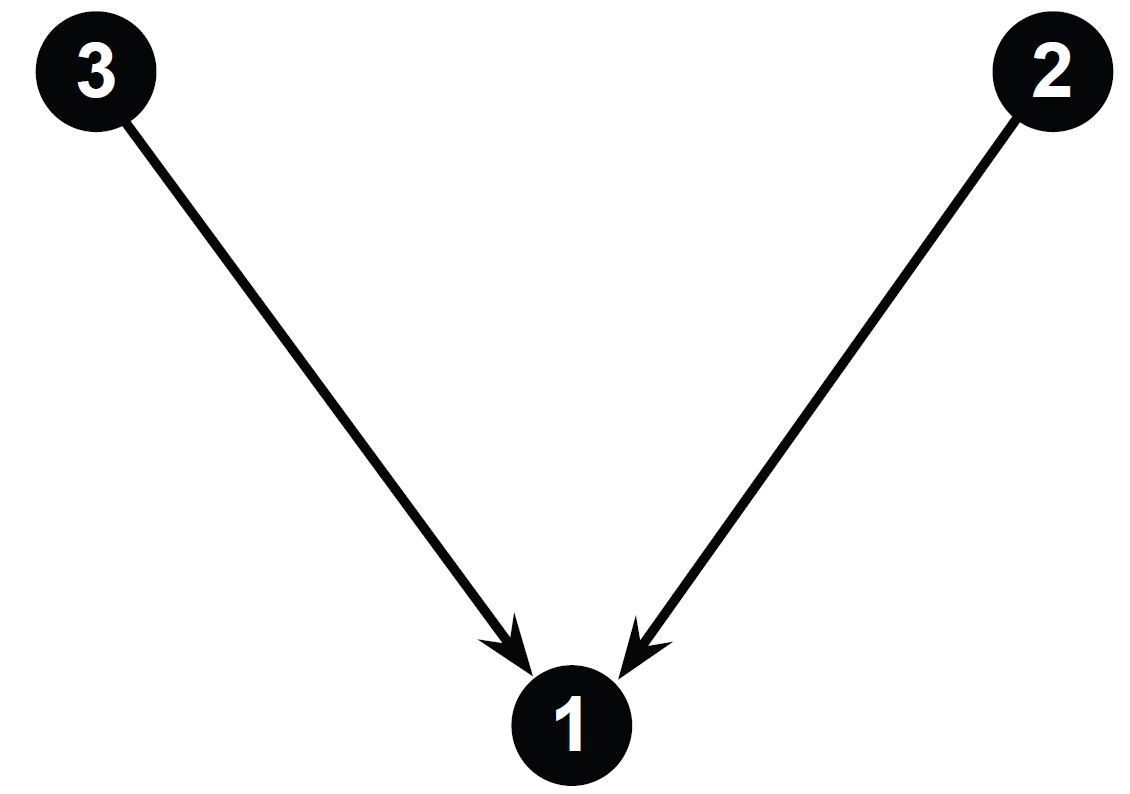
Figure 5: Wishart density w.r.t. a Hausdorff measure

Ex 7.1.

Consider DAG $\mathcal{D}$ given in Figure 5. The Jacobian matrix corresponding to (37) and (38) are given as follows:

$$M_{\psi}=\left(\begin{matrix}-D_{11}^{-2}&0&0&0&0\\ -L_{21}D_{11}^{2}&D_{11}^{-1}&0&0&0\\ -L_{21}^{2}D_{11}^{-2}&2L_{21}D_{11}^{-1}&-D_{22}^{-2}&0&0\\ -L_{31}D_{11}^{-2}&0&0&D_{11}^{-1}&0\\ -L_{31}^{2}D_{11}^{-2}&0&0&2L_{31}D_{11}^{-1}&0\\ -L_{21}L_{31}D_{11}^{-2}&L_{31}D_{11}^{-1}&0&L_{21}D_{11}^{-1}&-D_{33}^{-2}\\ \end{matrix}\right)$$

By computing $\det(M_{\psi}^{t}M_{\psi})$ we obtain

$$\mathbf{J}\psi(D,L)=D_{11}^{-4}D_{22}^{-2}D_{33}^{-2}\left(L_{31}^{4}+4L_{31}^{2}+1\right)^{1/2}.$$

Thus the density of $\pi_{U,\alpha}^{\mathrm{P}_{\mathcal{D}}}$ w.r.t. $\mathcal{H}^{5}$ on $\mathbb{R}^{6}$ is given by

$$z_{\mathcal{D}}(U,\alpha)^{-1}\exp\{-\frac{1}{2}\mathrm{tr}(\Omega U)\}D_{11}^{-\frac{\alpha_{1}}{2}+4}D_{22}^{-\frac{\alpha_{2}}{2}+2}D_{33}^{-\frac{\alpha_{3}}{2}+2}\left(L_{31}^{4}+4L_{31}^{2}+1\right)^{-1/2},$$

where $D_{ii}$ and $L_{ij}$ are considered as functions of $\Omega$.

Supplemental Section D: Computational algorithms and more related results

Completion algorithms for computing the DAG-constrained MLE and MAP of DAG-Wishart

Algorithm 7 (Maximum Likelihood).

Let $S$ denote the sample covariance matrix for $n$ i.i.d. observations and assume the sample size $n\geq\max\{pa_{i}+1:\>i\in V\}$. For each $i$ set

$$\lambda_{i}=S_{ii|\prec i\succ}\in\mathbb{R}_{+}\quad\text{and}\quad\boldsymbol{\beta}_{i}=S_{\prec i\succ}^{-1}S_{\prec i]}\in\mathbb{R}^{pa_{i}}.$$

Note that $\lambda_{i}=S_{ii}$ whenever $\mathrm{pa}(i)=\emptyset$. For $i=p,p-1,\cdots 1$:

1. Initialize $\widehat{\Sigma}_{ii}=\lambda_{i}$ for each $i$ such that $\mathrm{pa}(i)=\emptyset$ (in particular for $i=p$);

2. set $\widehat{\Sigma}_{\prec i]}=\widehat{\Sigma}_{\prec i\succ}\boldsymbol{\beta}_{i}$ if $\mathrm{pa}(i)\neq\emptyset$;

3. set $\widehat{\Sigma}_{ii}=\lambda_{i}+\boldsymbol{\beta}_{i}^{\top}\widehat{\Sigma}_{\prec i\succ}\boldsymbol{\beta}_{i}$ if $\mathrm{pa}(i)\neq\emptyset$;

4. set $\widehat{\Sigma}_{\nprec i]}=\widehat{\Sigma}_{\nprec i\succ}\widehat{\Sigma}_{\prec i\succ}^{-1}\widehat{\Sigma}_{\prec i]}$ if $\mathrm{pa}(i)\neq\emptyset$, otherwise set $\widehat{\Sigma}_{\nprec i]}=0$.

For the precision matrix $\Omega$, the MLE $\hat{\Omega}$ is just the inverse of $\hat{\Sigma}$.

Now we evaluate the performance of the posterior mode of the the DAG-Wishart prior, i.e., the maximum a posteriori (MAP). Since the DAG-Wishart prior is a conjugate prior for Gaussian DAG model, by slightly modifying Algorithm 7 we can compute the MAP for $\Sigma$, denoted by $\Sigma_{\textsc{{map}}}$ as follows:

Algorithm 8 (Posterior Mode).

Let $S$ denote the sample covariance matrix obtained from $n$ i.i.d. observations and assume the sample size $n\geq\max\{pa_{i}+1:\>i\in V\}$.

Initialization: For $i=1,\cdots,p$, set $\lambda_{i}=\frac{(nS+U)_{ii|\prec i\succ}}{\alpha_{i}+n},\beta_{i}=-((nS+U)_{\prec i\succ})^{-1}(nS+U)_{\prec i]}.$ By default, $\lambda_{i}=\frac{(nS+U)_{ii}}{\alpha_{i}+n},\beta_{i}=0$ whenever $\mathrm{pa}(i)=\emptyset$.

Compute: For $i=p,p-1,\cdots,1$, do step 1-4 in Algorithm 7.

Note that $\Omega_{\textsc{{map}}}$, the MAP for $\Omega$, is easily computed as the inverse of $\Sigma_{\textsc{{map}}}$.

Covariation Estimation using DAG-Wishart Estimators

The performance of the estimators of $\Sigma$ is shown in Table 4. A before, $p=500$ and the random graph edge proportion is 0.01. The hyperparameter setting $(3.5,I(3))$ gives the best among esitmatos among the hyperparameter choices. The differences however are not very large. Using the Bayes estimator $\widehat{\Sigma}_{\textsc{bayes}}$ is preferable under $L_{2}$ loss and $(\widehat{\Omega}_{\textsc{bayes}})^{-1}$ is the best under $L_{1}$ loss. As expected when the sample size is small, the risk reductions given by the Bayes estimators is more significant than in larger sample sizes.

		n=30		n=50		n=100
$(c,U)$	Estimator	$L_{1}$	$L_{2}$	$L_{1}$	$L_{2}$	$L_{1}$	$L_{2}$
$(2.5,I(3))$	$\widehat{\Sigma}_{\textsc{bayes}}$	-9.8%	4.6%	-8.0%	1.4%	-5.1%	0.2%
	$(\widehat{\Omega}_{\textsc{bayes}})^{-1}$	27.9%	-113.2%	17.4%	-100.2%	8.8%	-68.7%
	$\Sigma_{\textsc{{map}}}$	27.4%	-32.0%	17.4%	-27.0%	9.1%	-16.4%
$(3,I(3))$	$\widehat{\Sigma}_{\textsc{bayes}}$	1.0%	10.5%	-1.2%	5.4%	-1.4%	2.6%
	$(\widehat{\Omega}_{\textsc{bayes}})^{-1}$	30.1%	-130.6%	19.2%	-115.6%	10.0%	-79.4%
	$\Sigma_{\textsc{{map}}}$	27.1%	-45.2%	17.0%	-38.2%	8.8%	-23.6%
$(3.5,I(3))$	$\widehat{\Sigma}_{\textsc{bayes}}$	7.6%	12.3%	4.0%	6.8%	1.6%	3.4%
	$(\widehat{\Omega}_{\textsc{bayes}})^{-1}$	31.0%	-148.1%	19.9%	-131.7%	10.5%	-90.8%
	$\Sigma_{\textsc{{map}}}$	26.0%	-58.8%	15.9%	-50.1%	8.0%	-31.7%
$(3,I(2.5))$	$\widehat{\Sigma}_{\textsc{bayes}}$	7.9%	11.8%	4.5%	6.2%	2.0%	2.9%
	$(\widehat{\Omega}_{\textsc{bayes}})^{-1}$	30.8%	-141.6%	19.7%	-124.3%	10.4%	-84.7%
	$\Sigma_{\textsc{{map}}}$	24.6%	-49.2%	14.8%	-42.1%	7.3%	-26.6
$(3,I(3.5))$	$\widehat{\Sigma}_{\textsc{bayes}}$	-9.8%	8.2%	-8.7%	4.0%	-5.9%	1.8%
	$(\widehat{\Omega}_{\textsc{bayes}})^{-1}$	27.4%	-120.3%	16.9%	-107.6%	8.4%	-74.5%
	$\Sigma_{\textsc{{map}}}$	27.4%	-41.6%	17.4%	-34.6%	9.1%	-21.0%

Table 4: The relative improvements over MLE on $L_{1}$ and $L_{2}$ losses brought by Bayes estimators when estimating $\Sigma$. Here we fix $p=500$.

Role of sparsity and robustness to outliers

The previous results correspond to an underlying true graph with degree of sparsity (or edge proportion) equal to 0.01. We also investigate if the same hyperparameters work similarly well for graphs with different sparsity levels. Table 5 shows the relative improvement under different loss functions on graphs with edge proportion 0.005, 0.01, 0.015 and 0.02. All of the results use the configuration $c=3,u=3$. It can be seen that the sparsity of the graph is related to the performance of the estimators. In particular, even though $c=3,u=3$ constitute a good hyperparameters in the case of edge proportion 0.01, the same configuration does not work as well when the graph generating sparsity is increased to 0.015 or 0.02. In such denser situations, the Bayes estimators give better estimation only when the sample size is small (say, $n=30$). To achieve better performance, one has to use other hyperparameter configurations. One pattern that is seemingly odd is that as the sample size increases, the difference between the performance of the Bayes estimator and that of the MLE increases. This is unexpected, as when $n$ is larger enough, the performance of the MLE and the Bayes estimator should be essentially the same. The reason could be size that size $n=100$ is far from being “large enough”. All estimators have better estimation as we increase $n$ but in this small range $n$, the performance of MLE improves more quickly with the increasing sample size. Figure 6 shows the $L_{2}$ loss of estimators for $\Omega$ for various values of $n$ and when the edge proportion is 0.015.

		n=30		n=50		n=100
Edge proportion	Estimator	$L_{1}$	$L_{2}$	$L_{1}$	$L_{2}$	$L_{1}$	$L_{2}$
0.005	$\widehat{\Omega}_{\textsc{bayes}}$	33.7%	72.7%	21.4%	53.7%	11.3%	32.5%
	$(\widehat{\Sigma}_{\textsc{bayes}})^{-1}$	38.9%	68.3%	25.6%	51.0%	13.9%	31.8%
	$\Omega_{\textsc{{map}}}$	22.0%	62.2%	11.8%	41.5%	5.1%	22.3%
0.01	$\widehat{\Omega}_{\textsc{bayes}}$	39.2%	80.5%	24.7%	60.5%	12.9%	34.6%
	$(\widehat{\Sigma}_{\textsc{bayes}})^{-1}$	47.4%	65.9%	31.1%	39.9%	16.7%	13.8%
	$\Omega_{\textsc{{map}}}$	34.4%	81.5%	20.1%	62.3%	9.7%	37.7%
0.015	$\widehat{\Omega}_{\textsc{bayes}}$	45.1%	57.9%	23.2%	-34.5%	8.6%	-244.4%
	$(\widehat{\Sigma}_{\textsc{bayes}})^{-1}$	49.1%	45.8%	28.4%	-67.0%	8.3%	-307.8%
	$\Omega_{\textsc{{map}}}$	48.6%	64.3%	26.9%	-14.3%	12.4%	-198.2%
0.02	$\widehat{\Omega}_{\textsc{bayes}}$	38.1%	60.0%	-7.0%	-118.1%	-59.1%	-812.6%
	$(\widehat{\Sigma}_{\textsc{bayes}})^{-1}$	36.3%	58.7%	-13.3%	-124.7%	-68.4%	-834.4%
	$\Omega_{\textsc{{map}}}$	47.9%	60.8%	6.4%	-113.4%	-44.7%	-795.0%

Table 5: The relative improvement over MLE on $L_{1}$ and $L_{2}$ losses brought by Bayes estimators when estimating $\Omega$ in cases of different edge proportions. In small sample problems, the Bayes estimators is still preferable. But the performance of the MLE improves more quickly when the sample size increases. This indicates that the good hyperparameters for one particular sparsity might not be good if the sparsity changes.

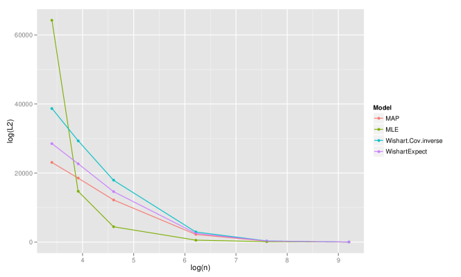
Figure 6: The $L_{2}$ loss for the estimators when $n$ increases. Here the sample proportion is 0.015.

We now proceed to test the robustness of the estimators to outliers. Instead of using purely Gaussian $\mathrm{N}(0,1)$ in the simulation, we add outliers of $\mathrm{N}(0,100)$ with probability 0.01 in the simulation. For the sake of comparison, we still use the same hyperparameter configurations as in the previous section, but focus on the improvements under such contaminated data.

The following Table 6 includes the relative improvement of the Bayes estimators over the MLE when outliers are included. Comparing with the previous pure Gaussian cases, it is clear that the improvements brought by the Bayes estimators become even more significant except on the $L_{2}$ loss on $\Sigma$, in which case the difference is very small. For instance, when $n=30,p=500$, the improvement on $L_{2}$ loss for the precision matrix is about 95% when outliers are included, compared with the improvement around 80% in the pure Gaussian case. This shows that the Bayes estimators are more robust to outliers (or in some sense, misspecification of distributions).

		n=30		n=50		n=100
Target	Estimator	$L_{1}$	$L_{2}$	$L_{1}$	$L_{2}$	$L_{1}$	$L_{2}$
$\Omega$	$\widehat{\Omega}_{\textsc{bayes}}$	65.1%	95.0%	50.9%	87.3%	32.2%	69.7%
	$(\widehat{\Sigma}_{\textsc{bayes}})^{-1}$	72.1%	95.2%	58.0%	89.7%	37.8%	75.0%
	$\widehat{\Omega}_{\textsc{map}}$	59.7%	93.3%	44.9%	83.3%	27.0%	63.4%
$\Sigma$	$\widehat{\Sigma}_{\textsc{bayes}}$	26.6%	9.2%	23.1%	4.6%	15.9%	1.6%
	$(\widehat{\Omega}_{\textsc{bayes}})^{-1}$	45.1%	-67.5%	34.3%	-40.2%	21.5%	-16.4%
	$\widehat{\Sigma}_{\textsc{map}}$	17.7%	-13.8%	28.6%	-5.4%	17.7%	-1.0%

Table 6: The relative improvement over MLE on $L_{1}$ and $L_{2}$ losses brought by Bayes estimators under $\mathrm{N}(0,100)$ outlier with probability 0.01. Here $p=500$ and $(c,U)=(3,I(3))$.

Call Center Data

The call center data comes from a major financial institute in 2002. It contains all the calls to the center in that year. The center was staffed from 7 a.m. each day until midnight. The weekends, holidays and misfunctioning days are excluded, so we have 239 days in total. In each day from 7 a.m. to midnight, we divided the time into 10-min intervals, and the number of calls are denoted by $N_{ij}$ where $i=1,\cdots 239$ and $j=1,\cdots,102$. A transformation $x_{ij}=\sqrt{N_{ij}+1/4}$ was applied to make the data closer to normal. Taking the 102 counts of time intervals as a vector, the data naturally contains a valid parent ordering, which is the time order. This is because it is not likely future counts could influence past.

The evaluation task here is the same as in [3] and [18] and so we follow their description of the problem for this example. The goal is to predict the call counts in the intervals of the second half of the day conditional on the first half day call counts. We used the conditional distribution as the predictor. Let $x_{i}=(x_{i}^{(1)},x_{i}^{(2)})$ be the $i$th observation, where $x_{i}^{(1)}=(x_{i,1},\cdots,x_{i,51})$ be the first half covariates and $x_{i}^{(2)}=(x_{i,52},\cdots,x_{i,102})$ be the second half. Then we partition the mean and covariance matrix in this way and obtain

$$\mu=\begin{bmatrix}\mu^{(1)}\\ \mu^{(2)}\\ \end{bmatrix},\Sigma=\begin{bmatrix}\Sigma_{11}&\Sigma_{12}\\ \Sigma_{21}&\Sigma_{22}\\ \end{bmatrix}.$$

The conditional expectation predictor is $\hat{x}^{(2)}=\mu^{(2)}+\Sigma_{21}\Sigma_{11}^{-1}(x^{(1)}-\mu^{(1)}).$ We use the first 10 months as the training data (205 observations in total )and the last 2 months (34 observations in total) as the test data. Then we estimate the mean and covariance from the training data. One baseline method is to use the naive MLE (denoted Naive-MLE), that is, the sample covariance matrix ignoring the potential underlying graphical structure. We can also use the constrained MLE after having estimated the graph structure using either the LassoDAG or the DAG-W method: these estimates are denoted by LassoDAG-MLE and DAG-W-MLE respectively. In addition, we include the Bayes estimator $(\widehat{\Omega}_{\textsc{bayes}})^{-1}$ given the model selection results from the DAG-W: we denote it as the DAG-W-Precision.

The prediction goal is a supervised task and one way to choose the hyperparameters can be cross-validation. However, to emphasize the effectiveness of our recommended hyper-parameter settings, here we use the recommended configurations $\kappa=0.1$ in LassoDAG and $c=1,b=3$ in DAG-W. In Figure 7, the average absolute errors for the 51 time intervals are shown, where we define the average absolute error as

$$E_{j}=\frac{1}{34}\sum_{i=1}^{34}|x_{ij}-\hat{x}_{ij}|,j=1,2,\cdots 51.$$

It can be seen (see Fig 7) that the DAG-W-MLE is nearly uniformly better than the LassoDAG-MLE and Naive-MLE, while the DAG-W-Precision is even better than the other three. Since the covariance estimation method is the same for LassoDAG-MLE and DAG-W-MLE, the difference indicates the advantage of model selection by DAG-W. DAG-W-Precision also involves Bayes shrinkage in addition to the model selection, resulting in additional benefits. LassoDAG is also better than MLE in most of the time intervals, thus we see that any model selection is better than no model selection at all.

Another way to measure performance is to treat each sample $x_{i}\in\mathbb{R}^{51}$ as one individual and take the $L_{2}$ errors for each day in test set

$$SSE_{i}=\|{x_{i}-\hat{x}_{i}}\|^{2}.$$

The MSE for each method is then estimated by the average of $SSE_{i}$ over all $i$ in test set. Table 7 shows the MSE from the three different methods of covariance estimation. It can be seen that DAG-W is much better than LassoDAG and naive MLE.

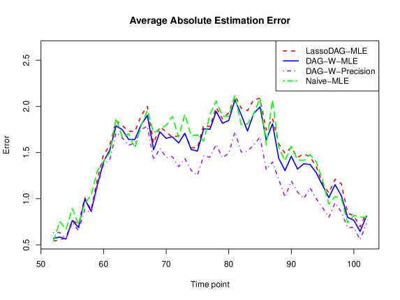
Figure 7: The average absolute errors for all 51 time intervals of second half of the day, from different predictions.

	Naive-MLE	LassoDAG-MLE	DAG-W-MLE	DAG-W-Precision
MSE	172.976	166.138	142.730	123.438

Table 7: Mean squared errors of predictions for the call center data given by different methods.

References

- [1] Steen A. Andersson and Michael D. Perlman. Normal linear regression models with recursive graphical Markov structure. J. Multivariate Anal., 66(2):133–187, 1998.
- [2] Emanuel Ben-David and Bala Rajaratnam. Positive definite completion problems for Bayesian networks. SIAM J. Matrix Anal. Appl., 33(2):617–638, 2012.
- [3] Peter J. Bickel and Elizaveta Levina. Regularized estimation of large covariance matrices. Ann. Statist., 36(1):199–227, 2008.
- [4] Patrick Billingsley. Probability and measure. John Wiley & Sons, New York-Chichester-Brisbane, 1979. Wiley Series in Probability and Mathematical Statistics.
- [5] A. P. Dawid and S. L. Lauritzen. Hyper-Markov laws in the statistical analysis of decomposable graphical models. Ann. Statist., 21(3):1272–1317, 1993.
- [6] Persi Diaconis, Kshitij Khare, and Laurent Saloff-Coste. Gibbs sampling, exponential families and orthogonal polynomials. Statistical Science, 23(2):151–178, 05 2008.
- [7] Jerome Friedman, Trevor Hastie, and Robert Tibshirani. Sparse inverse covariance estimation with the graphical lasso. Biostatistics, 9(3):432–441, 2008.
- [8] Dan Geiger and David Heckerman. Parameter priors for directed acyclic graphical models and the characterization of several probability distributions. Ann. Statist., 30(5):1412–1440, 2002.
- [9] Dan Geiger and David Heckerman. Learning gaussian networks. CoRR, abs/1302.6808, 2013.
- [10] Robert Grone, Charles R. Johnson, Eduardo M. de Sá, and Henry Wolkowicz. Positive definite completions of partial Hermitian matrices. Linear Algebra Appl., 58:109–124, 1984.
- [11] Alain Hauser and Peter Bühlmann. Characterization and greedy learning of interventional Markov equivalence classes of directed acyclic graphs. J. Mach. Learn. Res., 13:2409–2464, 2012.
- [12] Beatrix Jones, Carlos Carvalho, Adrian Dobra, Chris Hans, Chris Carter, and Mike West. Experiments in stochastic computation for high-dimensional graphical models. Statist. Sci., 20(4):388–400, 2005.
- [13] Markus Kalisch, Martin Mächler, Diego Colombo, Marloes H. Maathuis, and Peter Bühlmann. Causal inference using graphical models with the r package pcalg. Journal of Statistical Software, 47(11):1–26, 5 2012.
- [14] Kshitij Khare and Bala Rajaratnam. Wishart distributions for decomposable covariance graph models. Ann. Statist., 39(1):514–555, 2011.
- [15] Steffen L. Lauritzen. Graphical models, volume 17 of Oxford Statistical Science Series. The Clarendon Press, Oxford University Press, New York, 1996. Oxford Science Publications.
- [16] Gérard Letac and Hélène Massam. Wishart distributions for decomposable graphs. Ann. Statist., 35(3):1278–1323, 2007.
- [17] Judea Pearl and Nanny Wermuth. When can association graphs admit a causal interpretation? In P. Cheeseman and R.W. Oldford, editors, Selecting Models from Data, volume 89 of Lecture Notes in Statistics, pages 205–214. Springer New York, 1994.
- [18] Bala Rajaratnam, Hélène Massam, and Carlos M. Carvalho. Flexible covariance estimation in graphical Gaussian models. Ann. Statist., 36(6):2818–2849, 2008.
- [19] Alberto Roverato. Cholesky decomposition of a hyper inverse Wishart matrix. Biometrika, 87(1):99–112, 2000.
- [20] Karen Sachs, Omar Perez, Dana Pe’er, Douglas A. Lauffenburger, and Garry P. Nolan. Causal protein-signaling networks derived from multiparameter single-cell data. Science, 308(5721):523–529, 2005.
- [21] Ali Shojaie and George Michailidis. Penalized likelihood methods for estimation of sparse high-dimensional directed acyclic graphs. Biometrika, 97(3):519–538, 2010.
- [22] Nico M. Temme. Special functions : an introduction to the classical functions of mathematical physics. J. Wiley & sons, New York, 1996.
- [23] Nanny Wermuth. Linear recursive equations, covariance selection, and path analysis. J. Amer. Statist. Assoc., 75(372):963–972, 1980.