Flavor changing neutral currents in ttbar decays at DØ

Abstract

We present a search for flavor changing neutral currents (FCNC) in decays of top quarks. The analysis is based on a search for $t\bar{t}\rightarrow\ell^{\prime}\nu\ell\bar{\ell}$+jets ($\ell,\ell^{\prime}=e,\mu$) final states using 4.1 fb^-1 of integrated luminosity of $p\bar{p}$ collisions at $\sqrt{s}=1.96$ TeV. We extract limits on the branching ratio $B(t\rightarrow Zq)$ ($q=u,c$ quarks), assuming anomalous $tuZ$ or $tcZ$ couplings. We do not observe any sign of such anomalous coupling and set a limit of $B<3.2\%$ at 95% C.L.

I Introduction

In this paper, we search for FCNC decays of the top ($t$) quark topdecay . Within the standard model (SM) the top quark decays into a $W$ boson and a $b$ quark with a rate proportional to the Cabibbo-Kobayashi-Maskawa (CKM) matrix element squared, $|V_{\rm tb}|^{2}$ topdecay . Under the assumption of three fermion families and a unitary $3\times 3$ CKM matrix, the $|V_{\rm tb}|$ element is severely constrained to $|V_{\rm tb}|=0.999152^{+0.000030}_{-0.000045}$ pdg . While the SM branching fraction for $t\rightarrow Zq$ ($q=u,c$ quarks) is predicted to be $\approx 10^{-14}$ tZqfcnc , supersymmetric extensions of the SM with or without $R$-parity violation, or quark compositeness predict branching fractions as high as $\approx 10^{-4}$ tZqfcnc ; BSMtop1 ; fcnclhc . The observation of the FCNC decay $t\rightarrow Zq$ would therefore provide evidence of contributions from beyond SM (BSM) physics.

We analyze top-pair production ($t\overline{t}$), where either one or both of the top quarks decay via $t\rightarrow Zq$ or their charge conjugates (hereafter implied). Any top quark that does not decay via $t\rightarrow Zq$ is assumed to decay via $t\rightarrow Wb$. We assume that the $t\rightarrow Zq$ decay is generated by an anomalous FCNC term added to the SM Lagrangian

$${\cal L}_{\rm FCNC}=\frac{e}{2\sin\theta_{W}\cos\theta_{W}}\ \bar{t}\,\gamma_{\mu}(v_{tqZ}-a_{tqZ}\gamma_{5})\ q\,Z^{\mu}\,\,+h.c.,$$ (1)

where $q$, $t$, and $Z$ are the quantum fields for up or charm quarks, top quarks, and for the $Z$ boson, respectively, $e$ is the electric charge, and $\theta_{W}$ the Weinberg angle. We thereby introduce dimension-4 vector, $v_{tqZ}$, and axial vector, $a_{tqZ}$, couplings as defined in fcnc_coupling . We find in Refs. nloqcd1 ; nloqcd2 that the next-to-leading order (NLO) effects due to perturbative QCD corrections are negligible when extracting the branching ratio limits to the leading order (LO) in Eq. 1.

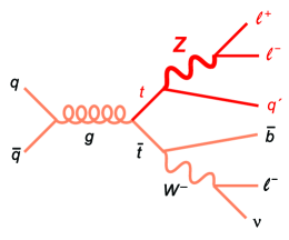
We investigate channels where the $W$ and $Z$ bosons decay leptonically, as shown in Fig. 1. The $u$, $c$, and $b$ quarks subsequently hadronize, giving rise to a final state with three charged leptons ($\ell=e,\mu$), an imbalance in momentum transverse to the $p\bar{p}$ collision axis ($E\kern-5.70007pt\raise 0.81805pt\hbox{/}_{T}$, assumed to be from the escaping neutrino in the $W\rightarrow\ell\nu$ decay), and jets.

Figure 1: Lowest-order diagram for FCNC $t\overline{t}\rightarrow WbZq^{\prime}$ production, where $q^{\prime}$ can be either a $u$ or $c$ quark, and the $W$ and $Z$ bosons decay leptonically.

This is the first search for FCNC in $t\bar{t}$ decays with trilepton final states. This mode provides a distinct signature with low background, albeit at the cost of statistical power. The first measurement ($b\rightarrow s\gamma$) was published in 1995 by the CLEO Collaboration cleo1995 . Numerous studies have been done since then to search for FCNC processes in meson decays, i.e., $b\rightarrow Zs$ in $B^{+}\rightarrow K^{*+}\ell^{+}\ell^{-}$ Bmeson_cdf ; Bmeson_belle ; Bmeson_babar , $B\rightarrow K^{*}\nu\bar{\nu}$ kamenik_arXiv , and $B_{s,d}\rightarrow\ell^{+}\ell^{-}$ Bmeson_artuso ; Bmeson_antonelli or $s\rightarrow Zd$ in $K^{+}\rightarrow\pi^{+}\nu\bar{\nu}$ Kmeson_e949 . Using the $D^{+}\rightarrow\pi^{+}\mu^{+}\mu^{-}$ final state in $1.3$ fb^-1 of integrated luminosity, the D0 Collaboration has set the best branching ratio ($B$) limits on the FCNC $c\rightarrow Zu$ process at $B(D^{+}\rightarrow\pi^{+}\mu^{+}\mu^{-})<3.9\times 10^{-6}$ at 90% C.L. fcnc_Dmeson . There are theoretical arguments as to why top quark decays may be the best way to study flavor violating couplings of mass-dependent interactions rsmodelitself ; fcnc_rsmodel . FCNC $tqZ$ and $tq\gamma$ couplings have been studied by the CERN $e^{+}e^{-}$ Collider (LEP), DESY $ep$ Collider (HERA), and Fermilab $p\bar{p}$ Collider (Tevatron) experiments fcnc_lep ; fcnc_h1 ; fcnc_zeus ; fcnc_tqgamma_cdf ; cdflimits . The D0 Collaboration has recently published limits on the branching ratios determined from FCNC gluon-quark couplings using single top quark final states d0glimits . The $95\%$ C.L. upper limit on the branching ratio of $t\rightarrow Zq$ from the CDF Collaboration uses 1.9 fb^-1 of integrated luminosity, assumes a top quark mass of $m_{\rm t}=175$ GeV and uses the measured cross section of $\sigma_{t\bar{t}}=8.8\pm 1.1$ pb cdflimits . This result excludes branching ratios of $B(t\rightarrow Zq)>3.7\%$, with an expected limit of 5.0% $\pm$ 2.2%. To obtain these results, CDF exploited the two lepton plus four jet final state. This signature occurs when one of the pair-produced top quarks decays via FCNC to $Zq$, followed by the decay $Z\rightarrow ee$ or $Z\rightarrow\mu\mu$. The other top quark decays to $Wb$, followed by the hadronic decay of the $W$ boson. This dilepton signature suffers from large background, but profits from more events relative to the trilepton final states investigated here.

This analysis is based on the measurement of the $WZ$ production cross section in $\ell\nu\ell\ell$ final states WZpub using 4.1 fb^-1 of integrated luminosity of $p\bar{p}$ collisions at $\sqrt{s}=1.96$ TeV. We extend the selection by analyzing events with any number of jets in the final state and investigate observables that are sensitive to the signal topology in order to select events with $WZ\rightarrow\ell\nu\ell\ell$ decays that originate from the pair production of top quarks.

II Object Reconstruction

An electron is identified from the properties of clusters of energy deposited in the central calorimeters (CC), end cap calorimeters (EC), or intercryostat detector (ICD) that match a track reconstructed in the central tracker. Because of the lack of far forward coverage of the tracker, we define EC electrons only within $1.5<|\eta|<2.5$. The calorimeter clusters in the CC and EC are required to pass the isolation cut

$$\frac{E_{\rm tot}(\Delta{\cal R}<0.4)-E_{\rm EM}(\Delta{\cal R}<0.2)}{E_{\rm EM}(\Delta{\cal R}<0.2)}<0.1$$

for “loose” electrons and $<0.07$ for “tight” electrons, where $E_{\rm tot}$ is the total energy in the EM and hadronic calorimeters, $E_{\rm EM}$ is the energy found in the EM calorimeter only, and $\Delta{\cal{R}}=\sqrt{(\Delta\phi)^{2}+(\Delta\eta)^{2}}$, where $\phi$ is the azimuthal angle. For the intercryostat region (ICR), $1.1<|\eta|<1.5$, we form clusters from the energy deposits in the CC, ICD, or EC detectors. These clusters are identified as electrons if they pass a neural network requirement that is based on the characteristics of the shower and associated track information. A muon candidate is reconstructed from track segments within the muon system that are matched to a track reconstructed in the central tracker. The trajectory of the muon candidate must be isolated from other tracks within a cone of $\Delta{\cal{R}}<0.5$, with the sum of the tracks’ transverse momenta, $p_{T}$, in a cone less than $4.0~{}{\rm GeV}$ for “loose” muons and less than $2.5~{}{\rm GeV}$ for “tight” muons. Tight muon candidates must also have less than $2.5~{}{\rm GeV}$ of calorimeter energy in an annulus of $0.1<\Delta{\cal{R}}<0.4$. Jets are reconstructed from the energy deposited in the CC and EC calorimeters, using the “Run II midpoint cone” algorithm RunIIcone of size $\Delta{\cal{R}}=0.5$, within $|\eta|<2.5$.

III Signal and Background Monte Carlo Simulations

Monte Carlo (MC) samples of $WZ$ and $ZZ$ background events are produced using the pythia generator pythia . The production of the $W$ and $Z$ bosons in association with jets ($W+$jets, $Z+$jets), collectively referred to as $V+$jets, as well as $t\bar{t}$ processes are generated using alpgen alpgen interfaced with pythia for parton evolution and hadronization. In all samples the CTEQ6L1 parton distribution function (PDF) set is used, along with $m_{\rm t}=172.5$ GeV. The $t\bar{t}$ cross section is set to the SM value at this top quark mass, i.e., $\sigma_{t\bar{t}}=7.46^{+0.48}_{-0.67}$ pb ttbar-cross-sec . This uncertainty is mainly due to the scale dependence, PDFs, and the experimental uncertainty on $m_{\rm t}$ top_wa .

All MC samples are passed through a geant geant simulation of the D0 detector and overlaid with data events from random beam crossings to account for the underlying event. The samples are then corrected for the luminosity dependence of the trigger, reconstruction efficiencies in data, and the beam position. All MC samples are normalized to the luminosity in data using NLO calculations of the cross sections, and are subject to the same selection criteria as applied to data.

The signal process is generated using the pythia generator with the decay $t\rightarrow Zq$ added. The $Z$ boson helicity is implemented by reweighting an angular distribution of the positively charged lepton in the decay $t\to Zq\to\ell^{+}\ell^{-}q$ using comphep comphep , modified by the addition of the Lagrangian of Eq. 1. The variable $\cos\theta^{*}$ used for the reweighting is defined by the angle $\theta^{*}$ between the $Z$ boson’s momentum in the top quark rest frame and the momentum of the positively charged lepton in the $Z$ boson rest frame. We assume in the analysis that the vector and axial vector couplings, as introduced in Eq. 1, are identical to the corresponding couplings for neutral currents (NC) in the SM, i.e., $v_{tuZ}=1/2-4/3\sin^{2}\theta_{W}=0.192$ and $a_{tuZ}=1/2$, where $\sin^{2}\theta_{W}=0.231$. To study the influence of different values of the couplings, we also analyse the following cases: (i.a) $v_{tuZ}=1,a_{tuZ}=0$; (i.b) $v_{tuZ}=0,a_{tuZ}=1$; and (ii) $v_{tuZ}=a_{tuZ}=1/\sqrt{2}$. As expected, the first two give identical results. The difference obtained by using cases (i), (ii), and using the values of the SM NC couplings is included as systematic uncertainty. Therefore, our result is independent of the actual values of $v_{tqZ}$ and $a_{tqZ}$. Since we do not distinguish $c$ and $u$ quark jets our results are valid also for $u$ and $c$ quarks separately.

The total selection efficiency, calculated as a function of $B=\Gamma(t\rightarrow Zq)/\Gamma_{\rm tot}$, where $\Gamma_{\rm tot}$ contains $t\rightarrow Wb$ and $t\rightarrow Zq$ decays only, can be written as

$$\epsilon_{t\bar{t}}=(1-B)^{2}\cdot\epsilon_{t\bar{t}\to W^{+}bW^{-}\bar{b}}+2B(1-B)\cdot\epsilon_{t\bar{t}\to ZqW^{-}\bar{b}}+B^{2}\cdot\epsilon_{t\bar{t}\to ZqZ\bar{q}},$$ (2)

where the efficiency $\epsilon_{t\bar{t}\to W^{+}bW^{-}\bar{b}}$ for the SM $t\bar{t}$ background contribution is used, along with the efficiencies $\epsilon_{t\bar{t}\to ZqW^{-}\bar{b}}$ and $\epsilon_{t\bar{t}\to ZqZ\bar{q}}$ that include the FCNC top quark decays.

IV Event Selection and Signal Acceptance

We consider four independent decay signatures: $eee+{\mbox{$E\kern-5.70007pt\raise 0.81805pt\hbox{/}_{T}$}}+X$, $ee\mu+{\mbox{$E\kern-5.70007pt\raise 0.81805pt\hbox{/}_{T}$}}+X$, $\mu\mu e+{\mbox{$E\kern-5.70007pt\raise 0.81805pt\hbox{/}_{T}$}}+X$, and $\mu\mu\mu+{\mbox{$E\kern-5.70007pt\raise 0.81805pt\hbox{/}_{T}$}}+X$, where $X$ is any number of jets. We require the events to have at least three lepton candidates with $p_{T}>15$ GeV that originate from the same $p\bar{p}$ interaction vertex and are separated from each other by $\Delta{\cal{R}}>0.5$. Jets are excluded from consideration unless they have $p_{T}>20$ GeV. We also require that the jets are separated from electrons by $\Delta{\cal{R}}>0.5$. There is no fixed separation cut between the muon and jets but the muon isolation requirement rejects most muons within $\Delta{\cal{R}}<0.4$ of a jet. The event must also have ${\mbox{$E\kern-5.70007pt\raise 0.81805pt\hbox{/}_{T}$}}>20$ GeV, which is calculated from the energy found in the calorimeter cells and $p_{T}$ corrected for any muons reconstucted in the event. Furthermore, all energy corrections applied to electrons and jets are propagated through to the $E\kern-5.70007pt\raise 0.81805pt\hbox{/}_{T}$.

Events are selected using triggers based on electrons and muons. There are several high-$p_{T}$ leptons from the decay of the heavy gauge bosons providing a total trigger efficiency for all signatures of $98\%\pm 2\%$.

To identify the leptons from the $Z$ boson decay, we consider only pairs of electrons or muons, additionally requiring them to have opposite electric charges. If no lepton pair is found within the invariant mass intervals of 74–108 GeV ($ee$), 65–115 GeV ($\mu\mu$) or 60–120 GeV ($ee$, with one electron in the ICR) the event is rejected, else, the pair that has an invariant mass closest to the $Z$ boson mass $M_{Z}$ is selected as the $Z$ boson. The lepton with the highest $p_{T}$ of the remaining muons or CC/EC electrons in the event is selected as originating from the $W$ boson decay. From simulation, this assignment of the three charged leptons to $Z$ and $W$ bosons is found to be $\approx$ 100% correct for $ee\mu$ and $\mu\mu e$, and about 92% and 89% for the $eee$ and $\mu\mu\mu$ channels, respectively.

Thresholds in the selection criteria are the same as in Ref. WZpub and the acceptance multiplied by efficiency results are summarized in Table 1 for the FCNC signal. These values are calculated with respect to the total rate expected for all three generations of leptonic $W$ and $Z$ decays.

Table 1: Final efficiencies in % including detector and kinematic acceptance as well as detector efficiencies for each decay signature as a function of jet multiplicity $n_{\rm jet}$. The efficiency, $\epsilon$, is defined assuming fully leptonic decays of the vector bosons from top quarks, as defined as in Eq. 2. The statistical and systematic uncertainties have been added in quadradure.

$n_{\rm jet}$	Inclusive	$0$	$1$	$\geq 2$
Channel	$\epsilon_{t\bar{t}\to ZqW^{-}\bar{b}}$ (%)
$eee$	$1.65\pm 0.24$	$(7.65\pm 1.45)\cdot 10^{-2}$	$0.57\pm 0.09$	$1.00\pm 0.15$
$ee\mu$	$1.92\pm 0.18$	$(6.77\pm 1.05)\cdot 10^{-2}$	$0.58\pm 0.06$	$1.17\pm 0.11$
$\mu\mu e$	$1.23\pm 0.13$	$(3.37\pm 0.73)\cdot 10^{-2}$	$0.34\pm 0.04$	$0.84\pm 0.10$
$\mu\mu\mu$	$1.48\pm 0.19$	$(3.05\pm 0.74)\cdot 10^{-2}$	$0.38\pm 0.06$	$1.06\pm 0.15$
Channel	$\epsilon_{t\bar{t}\to ZqZ\bar{q}}$ (%)
$eee$	$1.22\pm 0.18$	$(4.69\pm 0.68)\cdot 10^{-2}$	$0.41\pm 0.06$	$0.76\pm 0.11$
$ee\mu$	$3.75\pm 0.38$	$(1.07\pm 0.11)\cdot 10^{-1}$	$1.08\pm 0.11$	$2.56\pm 0.25$
$\mu\mu e$	$1.47\pm 0.16$	$(3.22\pm 0.57)\cdot 10^{-2}$	$0.38\pm 0.05$	$1.06\pm 0.32$
$\mu\mu\mu$	$2.76\pm 0.36$	$(3.63\pm 0.69)\cdot 10^{-2}$	$0.63\pm 0.09$	$2.10\pm 0.28$

V Data-Driven Backgrounds

In addition to SM $WZ$ production, the other major background is from processes with a $Z$ boson and an additional object misidentified as the lepton from the $W$ boson decay (e.g., from $Z+$jets, $ZZ$, and $Z\gamma$). A small background contribution is expected from processes such as $W+$jets and SM $t\bar{t}$ production. The $WZ$, $ZZ$, and $t\bar{t}$ backgrounds are estimated from the simulation, while the $V+$jets and $Z\gamma$ backgrounds are estimated using data-driven methods.

One or more jets in $V+$jets events can be misidentified as a lepton from $W$ or $Z$ boson decays. To estimate this contribution, we define a false lepton category for electrons and muons. A false electron is required to have most of its energy deposited in the electromagnetic part of the calorimeter and satisfy calorimeter isolation criteria for electrons, but have a shower shape inconsistent with that of an electron. A muon candidate is categorized as false if it fails isolation criteria, as determined from the total $p_{T}$ of tracks located within a cone $\Delta{\cal{R}}=0.5$ around the muon. These requirements ensure that the false lepton is either a misidentified jet or a lepton from the semi-leptonic decay of a heavy-flavor quark. Using a sample of data events, collected using jet triggers with no lepton requirement, we measure the ratio of misidentified leptons passing two different selection criteria, false lepton and signal lepton, as a function of $p_{T}$ in three bins, $n_{\rm jet}$ = 0, 1, and $\geq 2$, where $n_{\rm jet}$ is the number of jets. We then select a sample of $Z$ boson decays with at least one additional false lepton candidate for each final state signature. The contribution from the $V+$jets background is estimated by scaling the number of events in this $Z+$false lepton sample by the corresponding $p_{T}$-dependent misidentification ratio.

Initial or final state radiation in $Z\gamma$ events can mimic the signal process if the photon either converts into an $e^{+}e^{-}$ pair or is wrongly matched with a central track mimicking an electron and the $E\kern-5.70007pt\raise 0.81805pt\hbox{/}_{T}$ is mismeasured. As a result the $Z\gamma$ process is a background to the final state signatures with $W\to e\nu$ decays. To estimate the contribution from this background, we model the kinematics of these events using the $Z\gamma$ NLO MC simulation Baur . We scale this result by the rate at which a photon is misidentified as an electron. This rate is obtained using a data sample of $Z\to\mu\mu$ events containing a radiated photon, as it offers an almost background-free source of photons. The invariant mass $M(\mu\mu\gamma)$ is reconstructed and required to be consistent with the $Z$ boson mass. The $Z\rightarrow\mu\mu$ decay is chosen to avoid any ambiguity when assigning the electromagnetic shower to the final state photon candidate. As the $Z\gamma$ NLO MC does not model recoil jets, pythia MC samples are used to estimate $Z\gamma$ background jet multiplicities and $E\kern-5.70007pt\raise 0.81805pt\hbox{/}_{T}$. As the pythia samples do not contain events with final state radiation, we find the fraction of $Z\gamma$ events in data and pythia MC that pass our $E\kern-5.70007pt\raise 0.81805pt\hbox{/}_{T}$ cut and take the difference as a systematic uncertainty.

VI Results

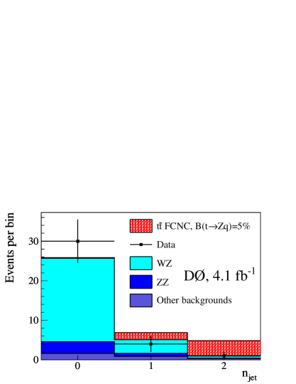
After all selection criteria have been applied, we observe a total of $35$ candidate events and expect $31.7\pm 0.3({\rm stat})\pm 3.9({\rm syst})$ background events from SM processes. The statistical uncertainty is due to MC statistics while the sources of systematic uncertainties are discussed later. Table 2 summarizes the number of events in each $n_{\rm jet}$ bin. The observed number of candidate and background events for each topology, summing over $n_{\rm jet}$, are summarized in Table 3. In Tables 2 and 3 and in all the following figures, we assume a $B$ of 5%.

Table 2: Number of observed events, expected number of $t\bar{t}$ FCNC events, and number of expected background events for each $n_{\rm jet}$ bin with statistical and systematic uncertainties. The MC statistical uncertainty on the $t\bar{t}$ signal is negligible, and we only present the systematic uncertainties. We assume $B=5\%$.

$n_{\rm jet}$	$0$	$1$	$\geq 2$
Background	$25.66\pm 0.28\pm 3.26$	$5.06\pm 0.14\pm 0.56$	$0.92\pm 0.08\pm 0.09$
$t\bar{t}\rightarrow WbZq$	$0.20\pm 0.03$	$1.80\pm 0.27$	$3.87\pm 0.56$
$t\bar{t}\rightarrow ZqZq$	$0.002\pm 0.001$	$0.020\pm 0.003$	$0.050\pm 0.007$
Observed	30	4	1

Table 3: Number of observed events, expected number of $t\bar{t}$ FCNC events, and number of expected background events for each final state signature with statistical and systematic uncertainties. The MC statistical uncertainty on the $t\bar{t}$ signal is negligible, and we only present the systematic uncertainties. We assume $B=5\%$.

Source	$eee$	$ee\mu$	$e\mu\mu$	$\mu\mu\mu$
$WZ$	$6.64\pm 0.07\pm 1.19$	$7.51\pm 0.08\pm 1.11$	$4.75\pm 0.06\pm 0.69$	$6.10\pm 0.07\pm 1.00$
$ZZ$	$0.33\pm 0.03\pm 0.06$	$1.76\pm 0.07\pm 0.17$	$0.46\pm 0.04\pm 0.07$	$1.30\pm 0.06\pm 0.21$
$V$ + jets	$0.60\pm 0.13\pm 0.11$	$0.40\pm 0.18\pm 0.17$	$0.48\pm 0.10\pm 0.01$	$0.22\pm 0.05\pm 0.03$
$Z\gamma$	$0.18\pm 0.05\pm 0.08$	$<0.001$	$0.66\pm 0.07\pm 0.38$	$<0.001$
$t\bar{t}\rightarrow WbWb$	$0.04\pm 0.01\pm 0.01$	$0.04\pm 0.01\pm 0.01$	$0.05\pm 0.01\pm 0.01$	$0.04\pm 0.01\pm 0.01$
Background	$7.89\pm 0.16\pm 1.20$	$9.71\pm 0.21\pm 1.14$	$6.40\pm 0.14\pm 0.79$	$7.66\pm 0.11\pm 1.02$
$t\bar{t}\rightarrow WbZq$	$1.57\pm 0.22$	$1.73\pm 0.17$	$1.17\pm 0.13$	$1.41\pm 0.18$
$t\bar{t}\rightarrow ZqZq$	$0.010\pm 0.001$	$0.029\pm 0.003$	$0.011\pm 0.001$	$0.022\pm 0.003$
Observed	8	13	9	5

To achieve better separation between signal and background, we analyze the $n_{\rm jet}$ and $H_{\rm T}$ distributions (defined as the scalar sum of transverse momenta of all leptons, jets, and $E\kern-5.70007pt\raise 0.81805pt\hbox{/}_{T}$), and the reconstructed invariant mass for the products of the decay $t\rightarrow Zq$.

The jet multiplicities in data, SM background, and in FCNC top quark decays are shown in Fig. 2.

Figure 2: Distribution of $n_{\rm jet}$ for data, for simulated FCNC $t\bar{t}$ signal, and for the expected background. The $ZqZq$ signal is included in the $t\bar{t}$ FCNC contribution but is expected to be small, as can be seen from Tables 2 and 3.

FCNC $t\bar{t}$ production leads to larger jet multiplicities and also a larger $H_{\rm T}$. This is shown in Fig. 3.

Figure 3: $H_{\rm T}$ distribution of data, FCNC $t\bar{t}$ signal, and expected background for events with (a) $n_{\rm jet}=0$, (b) $n_{\rm jet}=1$, and (c) $n_{\rm jet}\geq 2$.

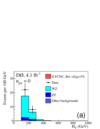
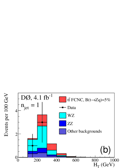
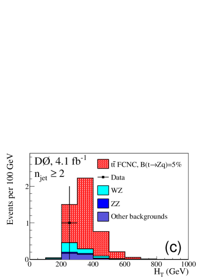
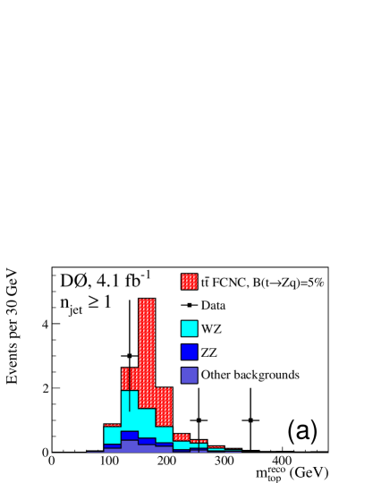
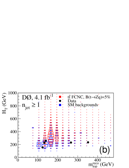
To further increase our sensitivity we reconstruct the mass of the top quark that decays via FCNC to a $Z$ boson and a quark ($t\rightarrow Zq$). In events with $n_{\rm jet}=0$, this variable is not defined. In events with one jet, we calculate the invariant mass, $m_{\rm t}^{\rm reco}\equiv M(Z,{\rm jet})$, from the 4-momenta of the jet and the identified $Z$ boson, to reconstruct $m_{\rm t}$. For events with two or more jets, we use the jet that gives a $m_{\rm t}^{\rm reco}$ closest to $m_{t}=172.5$ GeV. The $m_{\rm t}^{\rm reco}$ distribution is shown in Fig. 4(a). In Fig. 4(b), we present a 2-dimensional distribution of $m_{\rm t}^{\rm reco}$ and $H_{\rm T}$.

None of the observables in Figs. 2 – 4 show evidence for the presence of FCNC in the decay of $t\bar{t}$. We therefore set 95% C.L. limits on the branching ratio $B(t\rightarrow Zq)$. The limits are derived from 10 bins of the $H_{\rm T}$ distributions for $n_{\rm jet}=0,1$, and $\geq 2$. For the channels with $n_{\rm jet}=1$ and $n_{\rm jet}\geq 2$, we split each $H_{\rm T}$ distribution into 4 bins in $m_{\rm t}^{\rm reco}$, $m_{\rm t}^{\rm reco}<$ 120 GeV, 120 $<m_{\rm t}^{\rm reco}<$ 150 GeV, 150 $<m_{\rm t}^{\rm reco}<$ 200 GeV, and $m_{\rm t}^{\rm reco}>$ 200 GeV.

Figure 4: (a) $m_{\rm t}^{\rm reco}$ distribution of data, FCNC $t\bar{t}$ signal, and expected background for events with $n_{\rm jet}\geq 1$; (b) $H_{\rm T}$ vs. $m_{\rm t}^{\rm reco}$ distribution of data, FCNC $t\bar{t}$ signal, and background for events with $n_{\rm jet}\geq 1$.

VII Systematic Uncertainties

When calculating the limit on the branching ratio we consider several sources of systematic uncertainty. The systematic uncertainties for lepton-identification efficiencies are $15\%$ ($eee$), $11\%$ ($ee\mu$), $9\%$ ($\mu\mu e$), and $12\%$ ($\mu\mu\mu$). The systematic uncertainty assigned to the choice of PDF is $5\%$. In addition, we assign $9\%$ systematic uncertainty on $\sigma_{t\bar{t}}$ ttbar-cross-sec . This includes the dependence on the uncertainty of $m_{\rm t}$ top_wa . Furthermore, $m_{\rm t}$ is changed from $172.5$ GeV to $175$ GeV in $t\bar{t}$ MC samples with the difference in the result taken as a systematic uncertainty. We vary the $v_{tqZ}$ and $a_{tqZ}$ couplings as explained before Eq. 2, resulting in a 1% systematic uncertainty on the acceptance. Due to the uncertainty on the theoretical cross sections for $WZ$ and $ZZ$ production, we assign a $10\%$ vv-cross-sec systematic uncertainty to each. The major sources of systematic uncertainty on the estimated $V+$jets contribution arise from the $E\kern-5.70007pt\raise 0.81805pt\hbox{/}_{T}$ requirement and the statistics in the multijet sample used to measure the lepton-misidentification rates. These effects are estimated independently for each signature and found to be between $20\%$ and $30\%$. The systematic uncertainty on the $Z\gamma$ background is estimated to be $40\%$ and $58\%$ for the $eee$ and $\mu\mu e$ channels, respectively. Uncertainties on jet energy scale, jet energy resolution, jet reconstruction, and identification efficiency are estimated by varying parameters within their experimental uncertainties. For $n_{\rm jet}=0$ the uncertainty is found to be $1\%$, for $n_{\rm jet}=1$ it is $5\%$, and for $n_{\rm jet}\geq 2$ it is $20\%$. The measured integrated luminosity has an uncertainty of $6.1\%$ lumi .

VIII Limits Setting

We use a modified frequentist approach cls where the signal confidence level $CL_{s}$, defined as the ratio of the confidence level for the signal+background hypothesis to the background-only hypothesis ($CL_{s}=CL_{s+b}/CL_{b}$), is calculated by integrating the distributions of a test statistic over the outcomes of pseudo-experiments generated according to Poisson statistics for the signal+background and background-only hypotheses. The test statistic is calculated as a joint log-likelihood ratio (LLR) obtained by summing LLR values over the bins of the $H_{\rm T}$ distributions. Systematic uncertainties are incorporated via Gaussian smearing of Poisson probabilities for signal and backgrounds in the pseudo-experiments. All correlations between signal and backgrounds are maintained. To reduce the impact of systematic uncertainties on the sensitivity of the analysis, the individual signal and background contributions are fitted to the data, by allowing a variation of the background (or signal+background) prediction, within its systematic uncertainties collie . The likelihood is constructed via a joint Poisson probability over the number of bins in the calculation, and is a function of scaling factors for the systematic uncertainties, which are given as Gaussian constraints associated with their priors.

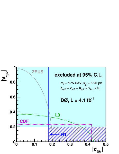
We determine an observed limit of $B(t\rightarrow Zq)<3.2\%$, with an expected limit of $<3.8\%$ at the 95% C.L. The limits on the branching ratio are converted to limits at the 95% C.L. on the FCNC vector, $v_{tqZ}$, and axial vector, $a_{tqZ}$, couplings as defined in Eq. 1 using the relation given in fcnc_coupling . This can be done for any point in the ($v_{tqZ}$, $a_{tqZ}$) parameter space and for different quark flavors ($u,c$) since the differences in the helicity structure of the couplings are covered as systematic uncertainties in the limit on the branching ratio. Assuming only one non-vanishing $v_{tqZ}$ coupling ($a_{tqZ}=0$), we derive an observed (expected) limit of $v_{tqZ}<0.19$ ($<0.21$) for $m_{t}=172.5$ GeV. Likewise, this limit holds assuming only one non-vanishing $a_{tqZ}$ coupling. Figure 5 shows current limits from experiments at the LEP, HERA, and Tevatron colliders as a function of the FCNC couplings $\kappa_{tu\gamma}$ (defined in Ref. fcnc_coupling ) and $v_{tuZ}$ for $m_{t}=175$ GeV.

Figure 5: Upper limits at the 95% C.L. on the anomalous $\kappa_{tu\gamma}$ and $v_{tuZ}$ couplings assuming $m_{t}=175$ GeV. Both D0 and CDF limits on $v_{tqZ}$ are scaled to the SM cross section of $\sigma_{t\bar{t}}=6.90$ pb ttbar-cross-sec . Anomalous axial vector couplings and couplings of the charm quark are neglected: $a_{tuZ}=v_{tcZ}=a_{tcZ}=\kappa_{tc\gamma}=0$. The scale parameter for the anomalous dimension-5 coupling $\kappa_{tu\gamma}$ is set to $\Lambda=m_{t}=175$ GeV fcnc_h1 . Any dependence of the Tevatron limits on $\kappa_{tu\gamma}$ is not displayed as the change is small and at most 6% for $\kappa_{tu\gamma}=0.5$. The domain excluded by D0 is represented by the light (blue) shaded area. The hatched area corresponds to the additional domain excluded at HERA by the H1 experiment fcnc_h1 . Also shown are upper limits obtained at LEP by the L3 experiment fcnc_lep (green dashed), at HERA by the ZEUS experiment fcnc_zeus (grey dashed), and at the Tevatron by the CDF experiment fcnc_tqgamma_cdf ; cdflimits (magenta dashed). The region above or to the right of the respective lines is excluded.

IX Conclusion

In summary, we have presented a search for top quark decays via FCNC in $t\bar{t}$ events leading to final states involving three leptons, an imbalance in transverse momentum, and jets. These final states have been explored for the first time in the context of FCNC couplings. In the absence of signal, we expect a limit of $B(t\rightarrow Zq)<3.8\%$ and set a limit of $B(t\rightarrow Zq)<3.2\%$ at the $95\%$ C.L. which is currently the world’s best limit. This translates into an observed limit on the FCNC coupling of $v_{tqZ}<0.19$ for $m_{t}=172.5$ GeV.

References

- (1) H. Fritzsch, Phys. Lett., B 224, 423 (1989).
- (2) K. Nakamura et al. (Particle Data Group), J. Phys. G 37, 075021 (2010).
- (3) J. A. Aguilar-Saavedra, Acta Phys. Polon. B 35, 2695 (2004).
- (4) F. Larios, R. Martinez and M. A. Perez, Phys. Rev. D 72, 057504 (2005).
- (5) P. M. Ferreira, R. B. Guedes and R. Santos, Phys. Rev. D 77, 114008 (2008).
- (6) T. Han and J. L. Hewett, Phys. Rev. D 60, 074015 (1999).
- (7) J. J. Zhang et al., Phys. Rev. Lett. 102, 072001 (2009). J. J. Zhang et al., Phys. Rev. D 82, 073005 (2010).
- (8) J. Drobnak et al., Phys. Rev. Lett. 104, 252001 (2010). J. Drobnak et al., Phys. Rev. D 82, 073016 (2010).
- (9) M. S. Alam et al. [CLEO Collaboration], Phys. Rev. Lett. 74, 2885 (1995).
- (10) T. Aaltonen et al. [CDF Collaboration], Phys. Rev. D 79, 011104(R) (2009).
- (11) J. T. Wei, P. Chang et al. [BELLE Collaboration], Phys. Rev. Lett. 103, 171801 (2009).
- (12) B. Aubert et al. [BaBar Collaboration], Phys. Rev. D 79, 031102(R) (2009).
- (13) J. Kamenik, arXiv:1012.5309
- (14) M. Artuso et al., Eur. Phys. J C 57, 309 (2008).
- (15) Antonelli et al., Phys. Rept. 494, 197 (2010).
- (16) S. Adler et al. [E949 Collaboration], Phys. Rev. D 77, 052003 (2008).
- (17) V. M. Abazov et al. [D0 Collaboration], Phys. Rev. Lett. 100, 101801 (2008).
- (18) L. Randall and R. Sundrum, Phys. Rev. Lett. 83, 3370 (1999).
- (19) S. Casagande et al., J. High Energy Phys. 10, 094 (2008).
- (20) P. Achard et al. [L3 Collaboration], Phys. Lett. B 549, 290 (2002); J. Abdallah et al. [DELPHI Collaboration], Phys. Lett. B 590, 21 (2004); A. Heister et al. [ALEPH Collaboration], Phys. Lett. B 543, 173 (2002); G. Abbiendi et al. [OPAL Collaboration], Phys. Lett. B 521, 181 (2001).
- (21) F. D. Aaron et al. [H1 Collaboration], Phys. Lett. B 678, 450 (2009).
- (22) S. Chekanov et al. [ZEUS Collaboration], Phys. Lett. B 559, 153 (2003).
- (23) F. Abe et al., Phys. Rev. Lett. 80, 2525 (1998).
- (24) T. Aaltonen et al. [CDF Collaboration], Phys. Rev. Lett. 101, 192002 (2008).
- (25) V. M. Abazov et al. [D0 Collaboration], Phys. Lett. B 693, 81 (2010).
- (26) V. M. Abazov et al. [D0 Collaboration], Phys. Lett. B 695, 67 (2011).
- (27) G. C. Blazey et al., in Proceedings of the Workshop: “QCD and Weak Boson Physics in Run II,” edited by U. Baur, R. K. Ellis, and D. Zeppenfeld, (Fermilab, Batavia, IL, 2000) p. 47; see Sec. 3.5 for details.
- (28) T. Sjöstrand, S. Mrenna, and P. Skands, J. High Energy Phys. 05, 026 (2006); we used V6.419 and tune A.
- (29) M. L. Mangano , J. High Energy Phys. 07, 1 (2003).
- (30) S. Moch and P. Uwer, Phys. Rev. D 78, 034003 (2008).
- (31) CDF and D0 Collaborations, arXiv:1007.3178 [hep-ex].
- (32) GEANT Detector Description and Simulation Tool, CERN Program Library Long Writeup W5013.
- (33) E. Boos et al. [CompHEP Collaboration], Nucl. Instrum. Meth. A 534, 250 (2004).
- (34) U. Baur and E. Berger, Phys. Rev. D 47, 4889 (1993).
- (35) J. M. Campbell and R. K. Ellis, Phys. Rev. D 60, 113006 (1999).
- (36) T. Andeen , FERMILAB-TM-2365 (2007).
- (37) T. Junk, Nucl. Instrum. Methods in Phys. Res. A 434, 435 (1999); A. Read, in ”1st Workshop on Confidence Limits,” CERN Report No. CERN-2000-005, 2000.
- (38) W. Fisher, FERMILAB-TM-2386-E.