Expansion velocity of a one-dimensional, two-component Fermi gas during the sudden expansion in the ballistic regime

Abstract

We show that in the sudden expansion of a spin-balanced, two-component Fermi gas into an empty optical lattice induced by releasing particles from a trap, over a wide parameter regime, the radius $R_{n}$ of the particle cloud grows linearly in time. This allow us to define the expansion velocity $V_{\mathrm{ex}}$ from $R_{n}=V_{\mathrm{ex}}t$. The goal of this work is to clarify the dependence of the expansion velocity on the initial conditions which we establish from time-dependent density matrix renormalization group simulations, both for a box trap and a harmonic trap. As a prominent result, the presence of a Mott-insulating region leaves clear fingerprints in the expansion velocity. Our predictions can be verified in experiments with ultra-cold atoms.

I Introduction

Research into the non-equilibrium properties of strongly correlated many-body systems has emerged into a dynamic and active field, driven by the possibility to address questions such as thermalization rigol08a ; polkovnikov11 , the properties of steady states, or state engineering in ultra-cold atomic gases bloch08 . While substantial theoretical attention has been devoted to quantum quenches in homogeneous systems polkovnikov11 , more recently, set-ups that give rise to finite particle or spin currents have been studied as well, both from the theoretical side rigol04 ; rigol05b ; rosch08 ; mandt11 ; hm08a ; hm09a ; muth12 ; hen10 ; jreissaty11 ; lundh11 ; delcampo06 ; delcampo08 and in experiments (see, e.g., Refs. anker05, ; kinoshita06, ; schneider11, ; medley11, ; sommer11b, ; joseph11, ). Using these approaches allows one to investigate transport properties of strongly correlated many-body systems - in and out-of-equilibrium - in cold atomic gases that are of great interest in condensed matter theory.

Our work is motivated by the experiment by Schneider et al. schneider11 who have studied the expansion of a two-component Fermi gas in an optical lattice in two and three dimensions (described by the Fermi-Hubbard model schneider08 ; joerdens08 ), starting from an almost perfect band insulator. The qualitative interpretation of their results is that, besides a ballistically propagating halo of particles, at finite interaction strengths a core of diffusively expanding particles exists schneider11 . In the case of one-dimensional (1D) bulk systems relevant for condensed matter problems and on the level of linear response theory, ballistic dynamics of interacting particles can be traced back to the existence of non-trivial conservation laws zotos97 . For instance, the fact that the energy current is conserved for the 1D Heisenberg model renders its spin transport ballistic away from zero total magnetization zotos97 ; transport1D ; rosch00 , whereas at zero magnetization there exists a quasi-local quantity prosen11 , which is conserved only for the infinite system, that gives rise to ballistic dynamics. While for the 1D Hubbard model, the understanding of its transport properties is by far less complete than for the Heisenberg chain, one might be tempted to expect similar quantities to play a role for the latter model as well zotos97 .

A qualitative difference between the sudden expansion in an optical lattice compared to steady-state transport measurements in condensed matter systems is that, in the latter case, the background density determines transport coefficients, whereas in the former case, the density itself becomes time-dependent schneider11 and all particles participate in the dynamics. As a consequence, in diffusive regimes, the dependence of the diffusion coefficient on density needs to be accounted for. In the ballistic case, as we shall see, the expansion velocity always depends on all momenta that are occupied in the initial state and not on just those close to the Fermi wave-vector. Therefore, a parameter regime complementary to condensed matter systems can be accessed with cold atoms.

Theoretical results for the expansion of interacting bosons or fermions in optical lattices are mostly available for the 1D case, for which exact numerical methods give access to at least the short time dynamics via the adaptive time-dependent density matrix renormalization group (tDMRG) method daley04 ; white04 ; schollwoeck05 ; schollwoeck11 or exact diagonalization (ED) rigol04 ; rigol05b . The richness of the non-equilibrium physics encountered in the expansion manifests itself in the observation of the dynamical emergence of coherence rigol04 ; rodriguez06 ; hm08a ; hen10 , which, for bosons, leads to the phenomenon of dynamical quasi-condensation rigol04 ; rodriguez06 ; hen10 and the intriguing phenomenon of the fermionization of the momentum distribution function (MDF) rigol05b ; minguzzi05 ; delcampo08 ; gritsev10 . In the case of a two-component Fermi gas, the short-time dynamics of the MDF and correlation functions hm08a , the emergence of metastable states hm09a ; muth12 and the time-evolution of density profiles for specific initial conditions have been investigated hm08a ; hm09a ; karlsson11 ; kajala11 ; kajala11a .

In the present work we study the 1D Hubbard model and we concentrate on the sudden expansion starting from initial states that are Mott insulators (MI), i.e., that have an integer filling of $n_{\mathrm{init}}=1$, Tomonaga-Luttinger (TL) liquids ($n_{\mathrm{init}}<1$), or systems in a harmonic trap. In the latter case, depending on filling and interaction strength, several phases may coexist in separate shells rigol04b . We analyze the dependence of the expanding cloud’s radius $R_{n}(t)$ on time $t$ and search for conditions to obtain ballistic dynamics, for which $R_{n}(t)=V_{\mathrm{ex}}\,t$ is a necessary criterion. In that case, the expansion velocity $V_{\mathrm{ex}}$ is a well-defined quantity, and, as a key result of our work, we clarify its dependence on the initial conditions.

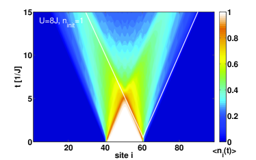
Figure 1: (Color online) Box trap: Typical contour plot of the density $\langle n_{i}(t)\rangle$ during the expansion from a MI ($U=8J$, $n_{\mathrm{init}}=1$, $L_{\mathrm{init}}=20$). The slanted lines indicate the speed $2J$ at which the MI melts.

Our main results are: (i) In the regime of low densities, i.e., $n_{\mathrm{init}}\leq 1$, we observe a linear growth of the cloud’s radius with time, allowing us to define $V_{\mathrm{ex}}$. (ii) In general, the expansion speed $V_{\mathrm{ex}}$ depends in a non-monotonic way on the initial density. In the case of the expansion from a MI, $V_{\mathrm{ex}}=\sqrt{2}J$, independently of $U$. (iii) Our findings are robust against the presence of a harmonic trap in the initial state.

Note that, in a generic system, one expects ballistic dynamics in the long time limit, where the gas becomes so dilute that interactions cease to matter. Here we show that ballistic dynamics sets in immediately after the gas is released from the trap when the density is actually still comparable to the initial density.

The structure of the paper is the following: In Section II, we introduce the model and define the radius of the cloud. Section III discusses the expansion from a box trap,i.e., starting from a homogeneous density. We first show that the dynamics is ballistic by analyzing the radius and the particle currents and second, we present a detailed analysis of the expansion velocity as a function of density and interaction strength. In Sec. IV we test our findings against the inhomogeneity introduced by a harmonic trap. We summarize our findings in Sec. V. In Appendix A, we discuss the diffusion equation in one dimension. Appendix B contains a finite-size analysis of the expansion velocity for various cases.

II Model and setup

Our study is carried out for the 1D Hubbard model:

$$H_{0}=-J\sum_{i=1,\sigma=\uparrow\downarrow}^{L-1}(c_{i+1,\sigma}^{\dagger}c_{i,\sigma}+\mathrm{h.c.})+U\sum_{i=1}^{L}n_{i,\uparrow}n_{i,\downarrow}\,.$$ (1)

$c_{i\sigma}^{\dagger}$ is a fermionic creation operator with spin $\sigma=\uparrow,\downarrow$ acting on site $i$, $n_{i\sigma}=c_{i\sigma}^{\dagger}c_{i\sigma}$, $n_{i}=\sum_{\sigma}n_{i\sigma}$, $U$ is the onsite repulsion, and $J$, is the hopping matrix element. Open boundary conditions are imposed, $L\gtrsim 100$. is the number of lattice sites, and $N$ the number of particles. We set $\hbar$ and the lattice spacing to unity and thus measure time, velocity and particle current in the appropriate units in terms of the hopping matrix element.

We prepare initial states as the ground state of $H=H_{0}+H_{\mathrm{conf}}$ hm08a . We consider two cases: First, the expansion from a box trap (i.e., $\langle n_{i}\rangle\not=0$ for $i_{1}<i\leq i_{2}$; $(i_{2}-i_{1})=L_{\mathrm{init}}$, $n_{\mathrm{init}}=N/L_{\mathrm{init}}$) enforced by using $H_{\mathrm{conf}}=\sum_{i}\epsilon_{i}n_{i}$ with a large $\epsilon_{i}\gtrsim U$ for $i\leq i_{1};i_{2}<i$ and zero otherwise). The second example is the expansion from a harmonic trap, for which $H_{\mathrm{conf}}=V\sum_{i}(i-i_{0})^{2}n_{i}$. We turn off $H_{\mathrm{conf}}$ at $t=0$. In our tDMRG runs, we use a Krylov-space based method park86 ; hochbruck97 , with time steps of $\delta t\,J=0.25$ and we enforce a discarded weight of $10^{-4}$ or smaller.

The main quantity of interest is the radius of the particle cloud that we define via

$$R_{n}=\sqrt{\frac{1}{N}\sum_{i=1}^{L}\langle n_{i}\rangle(i-i_{0})^{2}-R_{n}^{2}(t=0)}\,.$$ (2)

For the expansion from a box, $i_{0}=L/2+0.5$.

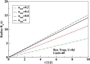
Figure 2: (Color online) Box trap: Radius $R_{n}(t)$ for initial densities $n_{\mathrm{init}}=0.2,0.4,0.8,1$ at $U=8J$ and $L_{\mathrm{init}}=40$ (corresponding to $N=8,16,32,40$).

III Expansion from a box trap

We first discuss this idealized case to avoid the complication of dealing with particles originating from different shells, as would be the case with a harmonic trap (note, though, that box-like traps can also be generated in experiments ashkin04 ; meyrath05 ). A typical example for the time-evolution of the density $\langle n_{i}(t)\rangle$ is shown in Fig. 1 for the expansion from a MI with $U=8J$. The MI melts on a time scale of $t_{\mathrm{melt}}\lesssim L_{\mathrm{init}}/(2J)$, where $2J$ is the largest possible velocity in the empty lattice, since the single-particle dispersion is $\epsilon_{k}=-2J\cos(k)$ hm08a . For $t>t_{\mathrm{melt}}$, two particle clouds form that propagate into opposite directions, visible as two intense jets (compare Refs. polini07 ; rigol04 ; rigol05b ; langer09 ; langer11 ; kajala11 ).

In Fig. 2, we display the radius $R_{n}(t)$ at $U=8J$ for various initial densities at $U=8J$. Clearly, for $n_{\mathrm{init}}\leq 1$, $R_{n}(t)=V_{\mathrm{ex}}t$. We stress that $R_{n}(t)\sim t$ sets in immediately after the gas is released from the trap. This includes, in particular, the expansion from a MI at any $U$, while for $n_{\mathrm{init}}>1$, the radius deviates from $R_{n}(t)\sim t$ hm09a . Based on the observation of $R_{n}(t)\sim t$ on short and intermediate times, when local densities are still large, together with the fact that interacting particles behave similar to non-interacting ones (which, in the absence of disorder, expand with $R_{n}\sim t$), we classify the dynamics as ballistic.

In our situation, the notion of ballistic dynamics is strongly corroborated by analyzing the time dependence of the total particle current in each half of the system, $J_{L/2}=\sum_{i>L/2}j_{i}$ [$j_{i}=-iJ\sum_{\sigma}(c_{i+1\sigma}^{\dagger}c_{i\sigma}-\mbox{h.c.})$], which is shown for $U/J=2,8$ in Fig. 3. After the two jets in Fig. 1 are well separated from each other, $J_{L/2}$ takes a constant value, which we consider a hallmark feature of ballistic dynamics langer11 .

However, in one dimension, there is a subtlety as certain solutions of the diffusion equation can also give rise to a linear increase of the radius with time (if properly defined). Such a scenario happens in the dilute limit (which we do not study here), yet it results in a strong dependence of the expansion velocity on the total particle, which is clearly different from our case as we shall see below. Further details are given in Appendix A.

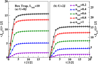
Figure 3: (Color online) Box trap: Total particle current in each half of the system as a function of time, i.e., $J_{L/2}(t):=\sum_{i>L/2}j_{i}$, for (a) $U=8J$, (b) $U=2J$ and $n_{\mathrm{init}}=0.2,0.4,0.6,0.8,1$. We observe that after some transient dynamics, $\langle J_{L/2}(t)\rangle=\mathrm{const}$, supporting the observation of ballistic transport.

The observation of a linear increase of the cloud radius with time implies that $V_{\mathrm{ex}}$ should be fully determined by properties of the initial state, such as the MDF, energy per particle, or density. In the non-interacting case, this is obvious, since $V_{\mathrm{ex}}$ can be calculated from the knowledge of the MDF. To guide the interpretation of the interacting case and to understand the dependence of $V_{\mathrm{ex}}$ on $U$ and $n_{\mathrm{init}}$, we next study the two exactly solvable limits $U=0$ and $U=\infty$.

III.1 Box trap, $V_{\mathrm{ex}}$ at $U=0$

At $U=0$, opening the trap simply means that particles will propagate with a velocity $v_{k}=2J\sin(k)$ with a probability given by the MDF $n_{k}$ in the initial state, which is $n_{k}=(1/N)\sum_{l,m,\sigma}e^{-i(l-m)k}\langle c^{\dagger}_{l\sigma}c_{m\sigma}\rangle\,$. The momenta are chosen to match the open boundary conditions in the box, i.e., $k=\frac{\pi l}{L_{\mathrm{init}}+1};l=1,\dots,L_{\mathrm{init}}$. By a straightforward evaluation of $R_{n}^{2}(t)$ from Eq. (2) and using the time-dependence of creation and annihilation operators, known exactly at $U=0$, we obtain $V_{\mathrm{ex}}$ as the average velocity of all particles in the initial state:

$$V_{\mathrm{ex}}^{2}=\frac{1}{N}\sum_{k}v_{k}^{2}\,n_{k}\,.$$ (3)

In the $U=0$ case, the initial MDF thus completely determines the expansion velocity. However, this is an over-complete set of constraints: For a very large $N$, where boundary conditions cease to matter, we can evaluate Eq. (3) analytically:

$$V^{2}_{\mathrm{ex}}=2J^{2}[k_{F}-\cos(k_{F})\sin(k_{F})]/k_{F}\,,$$ (4)

which yields the full dependence on the initial density at $U=0$ through $k_{F}\propto n_{\mathrm{init}}$ alone. We can interpret Eq. (4) in two ways: If $U=0$, $k_{F}=\pi n_{\mathrm{init}}/2$, whereas for $U=\infty$, $k_{F}=\pi n_{\mathrm{init}}$. Using ED, we have verified the validity of Eq. (4) by extracting $V_{\mathrm{ex}}$ from the time-dependence of $R_{n}(t)$ for $N\sim 160$ (see Fig. 8 in Appendix B).

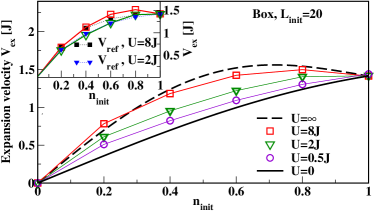
Figure 4: (Color online) Box trap: Main panel: $V_{\mathrm{ex}}$ vs $n_{\mathrm{init}}$ at $U/J=0,0.5,2,8,\infty$ for $L_{\mathrm{init}}=20$ [see the legend, symbols are tDMRG, the solid and the dashed lines are derived from Eq. (4)]. Inset: $V_{\mathrm{ex}}$ from tDMRG (open squares: $U=8J$, open triangles: $U=2J$) vs. $V_{\mathrm{ref}}$ (solid symbols) from non-interacting reference systems at a finite temperature (see Sec. III.3 for details)

III.2 Box trap, $V_{\mathrm{ex}}$ at $U\not=0$

In the interacting case, we extract the expansion velocity $V_{\mathrm{ex}}$ from the tDMRG data (i.e., the slope of curves such as the ones shown in Fig. 2). The results for selected values of $U$ are collected in the main panel of Fig. 4 (symbols). We emphasize four main observations: (i) For the expansion from the MI, we obtain $V_{\mathrm{ex}}=\sqrt{2}J$ at any $U>0$. (ii) At a fixed density, $V_{\mathrm{ex}}$ increases monotonically with $U$. (iii) For $U>4J$, the maximum of the expansion velocity is at an incommensurate density $0.5<n_{\mathrm{init}}<1$. (iv) The expansion velocity is always very different from characteristic velocities of the initial state and much smaller than $2J$, the largest possible velocity. It is also much smaller than the charge velocity giamarchi at small densities and at $n_{\mathrm{init}}=1$, where the charge velocity drops to zero, $V_{\mathrm{ex}}$ remains finite.

At $U=0$, the first observation is a consequence of particle-hole symmetry, reflected in the MDF: $n_{k}$ is point-symmetric about the point $(k_{F}=\pi/2,n_{k_{F}})$. Since $v^{2}_{k_{F}+\delta k_{F}}=v^{2}_{k_{F}-\delta k_{F}}$, from Eq. (3), we conclude $V_{\mathrm{ex}}=\sqrt{2}J$. The MDF at $U>0$ has the same symmetry property, hence we expect a similar behavior, confirmed by tDMRG. Of course, Eq. (3) does not directly apply to the interacting case. Since the total energy $E_{U}=\langle H_{0}\rangle$ is conserved, for $U>0$, Eq. (3) is incompatible with this initial condition set by $U>0$ and $n_{\mathrm{init}}$. However, we shall see that the observation of $V_{\mathrm{ex}}=\sqrt{2}J$ for $U>0$ can also be understood as a consequence of symmetry properties.

We can further use the exact result Eq. (4) to explain the observations (ii)-(iv). The $U=0$ and the $U=\infty$ result are the solid and the dashed lines in the main panel of Fig. 4, respectively, and therefore, increasing $U$ from $U=0$ to $U=\infty$ at a fixed density simply takes us from the limit of a non-interacting two-component Fermi gas to the limit of non-interacting spinless fermions. To understand that the maximum of $V_{\mathrm{ex}}$ is at an incommensurate $n_{\mathrm{init}}$ for $U>4J$, one needs to take into account that on the one hand, in a 1D cosine band, the maximum velocity is at $k=\pi/2$, but on the other hand, the density of states takes its minimum there. As a consequence of this competition, i.e., the decrease of $v_{k}$ vs the increase of the density of states as one moves away from $\pi/2$, the largest expansion velocity is at $n_{\mathrm{init}}\not=1$. Finally, property (iv) is a consequence of all particles propagating and not just those with momenta close to $k_{F}$.

On a technical note, we have checked the dependence of $V_{\mathrm{ex}}$ on particle number, keeping $n_{\mathrm{init}}=N/L_{\mathrm{init}}$ fixed. Finite-size effects are the largest at small initial densities, yet for densities $n_{\mathrm{init}}\gtrsim 0.5$, our tDMRG results obtained with $L_{\mathrm{init}}=40$ show little quantitative differences compared to smaller $L_{\mathrm{init}}$ and $V_{\mathrm{ex}}$ becomes independent of $N$ as shown in Appendix B.

III.3 Reference systems

It is now a compelling question to ask how many constraints suffice to determine the expansion velocity. From the solution of the non-interacting case, we conclude that density and energy are relevant quantities. To check this conjecture for the interacting case, we construct non-interacting reference systems that are at a finite temperature rosch-comm . The temperature is chosen such that the reference system has the same energy as the interacting system and the same particle number, and it lives in the same box potential of length $L_{\mathrm{init}}$.

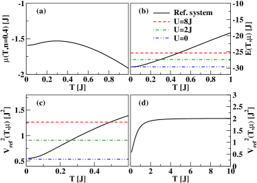
Figure 5: (Color online) These plots illustrate how the non-interacting reference systems are constructed using Eqs. (5), (6) and (7) for the example of $n_{\mathrm{init}}=0.4$ for (a),(b),(c): $L_{\mathrm{init}}=40$ and (d): $L_{\mathrm{init}}=160$: (a) Temperature dependence of the chemical potential at fixed $n_{\mathrm{init}}=0.4$. (b) Total energy from Eq. (6) as a function of temperature. (c) $V_{\mathrm{ref}}^{2}$ as a function of temperature. The horizontal lines in (b) are DMRG results for $E_{U}$ for the initial states used in the expansion at zero temperature for $U=0,2J,8J$, while in (c) they mark the resulting $V^{2}_{\mathrm{ref}}=V^{2}_{\mathrm{ref}}(E,n)$. (d) As $T$ increases, $V_{\mathrm{ref}}^{2}\to 2J^{2}$ from below, i.e., this is the largest expansion velocity that the reference systems can produce for $n_{\mathrm{init}}\leq 1$.

Hence we solve this set of equations:

$$N = \sum_{k,\sigma}f(\epsilon_{k}-\mu,T)\,,$$ (5)

$$E_{U} = \sum_{k,\sigma}\epsilon_{k}f(\epsilon_{k}-\mu,T)\,,$$ (6)

$$V_{\mathrm{ref}}^{2} = \frac{1}{N}\sum_{k,\sigma}v_{k}^{2}f(\epsilon_{k}-\mu,T)\,,$$ (7)

where $f(x,T)$ is the Fermi function. We proceed as illustrated in Fig. 5: For a given $U$ and $N$, we compute the total energy $E_{U}$ in the initial state with DMRG. First, we find the chemical potential $\mu=\mu(T)$ from Eq. (5), which only depends on $N$. Using this $\mu(T)$ curve, we determine the pair of $(\mu,T)$, for which we get the right energy $E_{U}$. From these results, Eq. (7) yields the expansion velocity $V_{\mathrm{ref}}$ of the reference system. Obviously, the maximum velocity that these reference systems, which have the dispersion $\epsilon_{k}=-2J\cos(k)$ of the empty lattice, can produce is $V_{\mathrm{ref}}=\sqrt{2}J$ at any density $n_{\mathrm{init}}\leq 1$ as $T\to\infty$. Within that constraint, the agreement between $V_{\mathrm{ex}}$ and our reference systems is excellent, as we illustrate for $U/J=2$ and $8$ in the inset of Fig. 4: Apart from those densities for which, at $U=8J$, $V_{\mathrm{ex}}>\sqrt{2}J$, $V_{\mathrm{ref}}\approx V_{\mathrm{ex}}$ within our numerical accuracy. In the particular case of $n_{\mathrm{init}}=1$, our reference systems also yield $V_{\mathrm{ref}}=\sqrt{2}J$ independently of $E_{U}$, consistent with the tDMRG results of Fig. 4. This is a consequence of the aforementioned symmetry property of the MDF, which also applies to $T>0$.

IV Expansion from a harmonic trap

Our results so far establish a relation between properties of the initial state and the expansion velocity that could be probed in experiments. We next test the robustness of our predictions for $V_{\mathrm{ex}}=V_{\mathrm{ex}}(U,n_{\mathrm{init}})$ against the inhomogeneity induced by a harmonic potential.

We focus on three types of initial states: (i) Only a TL, i.e., $\langle n_{i}\rangle<1$ in the entire trap, (ii) a MI shell in the center, surrounded by TL wings, and (iii) a three-shell structure with an incommensurate density in the center $\langle n_{i}\rangle>1$, surrounded by first, a MI shell and second, a TL shell with $\langle n_{i}\rangle<1$. For a given $U>0$, these regimes are separated by critical characteristic densities $\rho_{1}$ and $\rho_{2}$, where $\rho=N\sqrt{V/J}$ is the effective density in a system with a harmonic trap bloch08 ; rigol04b .

For all three cases, $R_{n}(t)$ is shown in Fig. 6 for $U/J=2$ and $8$. We observe that, after releasing the particles from the harmonic trap, the cloud still expands with $R_{n}(t)\sim t$ in cases (i) and (ii), i.e., $R_{n}(t)\sim t$ [see Fig. 6 (a) and (b)] whereas in case (iii), the increase of the radius is slower than linear in $t$ [see Fig. 6 (c) and (d)]. In that regime and for $U>4J$, the system can be viewed as a mixture of single atoms propagating with velocities $v_{k}\sim J$ and two fermions repulsively bound into a doublon, which, due to energy conservation, does not decay on time scales $\propto 1/J$ and is much slower with typical velocities $v_{k}^{d}\sim J^{2}/U$ kinoshita06 ; hm09a . For illustration, the values of $\rho_{1}$ and $\rho_{2}$ as well as typical density profiles are included in Fig. 7 for $U=8J$ (vertical lines and lower insets, respectively). As is evident from Fig. 7, the overall dependence of $V_{\mathrm{ex}}=V_{\mathrm{ex}}(\rho)$ resembles that of the expansion from a box trap, with a maximum in $V_{\mathrm{ex}}$ emerging as $U\gtrsim 4J$. Most importantly, as soon as the MI forms in the center of the trap, indicated by the vertical solid line at $\rho=\rho_{1}$, the expansion velocity approaches a constant value at $V_{\mathrm{ex}}\gtrsim\sqrt{2}J$ from above. The contribution to $V_{\mathrm{ex}}$ of low-density shells surrounding the MI is suppressed by increasing $U$ or $\rho$ since both favor a large relative fraction of all particles in the MI shell to minimize the contribution from the interaction energy. In contrast to the expansion from the box, the limit of $U=\infty$ (dashed line) is approached very slowly since the shell structure in a trap depends strongly on $U$ and $\rho$.

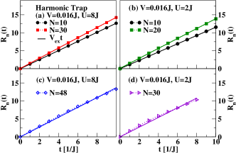
Figure 6: (Color online) Harmonic trap: Radius of the particle cloud for the expansion from a harmonic trap for (a) $N=10,30$ at $U=8J$, (b) $N=10,20$ at $U=2J$, (c) $N=48$ at $U=8J$ and (d) $N=30$ at $U=2J$. For $U=8J$, these parameters correspond to the initial states shown in the insets of Fig. 7. The solid lines are fits to the data, dotted lines are guides to the eye. We find $R_{n}(t)\not\sim t$ whenever densities in the center of the trap are larger than one and $R_{n}(t)\sim t$ otherwise.

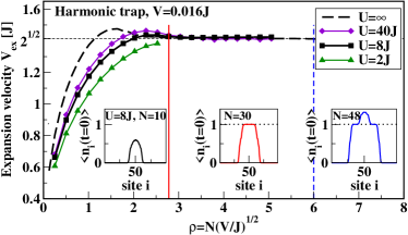
Figure 7: (Color online) Harmonic trap: $V_{\mathrm{ex}}$ vs $\rho$ ($U/J=2,8,40,\infty$, $V=0.016J$). The vertical solid line marks the formation of a MI shell in the trapped system at $\rho_{1}$ and the vertical dashed line the formation of a core with $\langle n_{i}\rangle>1$ at $\rho_{2}$, both for $U=8J$. The horizontal line is $V_{\mathrm{ex}}=\sqrt{2}J$. Symbols are tDMRG results, the dashed line was obtained from ED. We have verified that the results are remarkably stable against changes in the particle number at fixed $\rho$ by producing the $V_{\mathrm{ex}}=V_{\mathrm{ex}}(\rho)$ curve at a different $V$ (see Fig. 10 in Appendix B). Lower insets: typical initial density profiles in the regimes $\rho<\rho_{1}$, $\rho_{1}<\rho<\rho_{2}$ and $\rho_{2}<\rho$ for $U=8J$.

V Summary

We studied the sudden expansion of a spin-balanced two-component gas in 1D, released from a trap. Our main results are two-fold: First, the cloud expands ballistically as long as initial densities are small, including, in particular, the MI state. Second, the expansion velocity, defined through $R_{n}(t)=V_{\mathrm{ex}}t$ strongly depends on initial density and thus, its measurement can provide information on the initial state. For instance, deviations from our predictions could indicate the presence of defects in the initial state preparations. Our quantitative predictions can be tested in an experiment that realizes the set-up of Ref. schneider11 in 1D.

Furthermore it would be interesting to study the radius of an expanding cloud and the expansion velocity for other experimentally relevant systems such as the Bose-Hubbard model or spin imbalanced mixtures. While we have presented phenomenological evidence for ballistic dynamics, we have here not touched upon a potential relation with integrability and non-trivial conservation laws zotos97 , leaving this for future research. It also remains as an open question to identify interacting models in one dimension and parameter regimes in which diffusive dynamics dominates during the sudden expansion, which might be challenging since even non-integrable models may have very large conductivities (see, e.g., Ref. rosch00 ).

Appendix A: Linear increase of the radius from a nonlinear diffusion equation

Here we discuss solutions of the diffusion equation in one dimension in the limit of a very dilute gas. Since the sudden expansion scenario considered in this paper involves the propagation of all particles, the dependence of the diffusion constant $D$ on the local density $n(x,t)$ becomes relevant, and as a consequence, the relevant diffusion equation is in general a nonlinear one (see, e.g., schneider11 ). Focussing on the very dilute limit we use $D\sim 1/n(x,t)$ (see the discussion in Ref. schneider11 ; footnotediff ). The resulting diffusion equation (after rescaling of the time variable ):

$$\partial_{t}n(x,t)=\partial_{x}\frac{1}{n}\partial_{x}n\,,$$ (8)

has a self-similar solution with particle number conservation in 1D Vazquez06 :

$$n(x,t)=\frac{2t}{x^{2}+v^{2}t^{2}}\,.$$ (9)

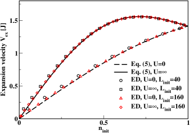
Figure 8: (Color online) Box trap: Comparison between the exact result for $V_{\mathrm{ex}}$ [Eq. (4) of the main text, valid in the limit of large particle numbers] and exact diagonalization in the limits $U=0$ and $U=\infty$. ED data are shown for $L_{\mathrm{init}}=40$ and $L_{\mathrm{init}}=160$. In the latter case, we find very good agreement between the analytical result (lines) and the ED data (symbols) for all densities.

First of all, one realizes that our definition of the radius $R_{n}(t)$, Eq. (2), cannot be used here. In the analysis of experimental data, it is common practice to define the radius as the half-width at half-maximum of the expanding cloud schneider11 . Using this definition, the solution Eq. (9) yields indeed $R_{n}(t)=vt$, similar to the ballistic dynamics discussed in our work. We would like to stress, though, that the sudden expansion described in the main text is genuinely different in some important respects. First, Eq. (8) is only valid in the dilute limit while the time-dependent DMRG gives us access to short and intermediate time-scales only where the gas is not necessarily a dilute one yet. Second, Eq. (9) is a solution for which the expansion velocity $v$ depends strongly on the particle number via $N=\int_{-\infty}^{\infty}n(x,t)dx=2\pi/v$, which is not observed in our case (compare Fig. 4 and 9). Based on these differences, we conclude that diffusive dynamics is very unlikely to be realized for the 1D Hubbard model in the sudden expansion.

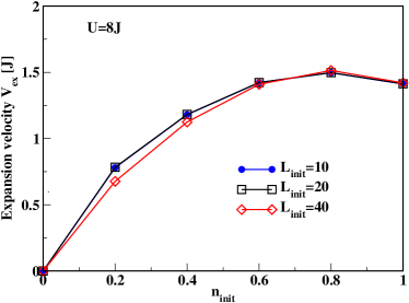
Figure 9: (Color online) Box trap: Expansion velocity as a function of initial density for $U=8J$ and different $L_{\mathrm{init}}=10,20,40$. For $n_{\mathrm{init}}\gtrsim 0.6$, finite-size effects are remarkably small.

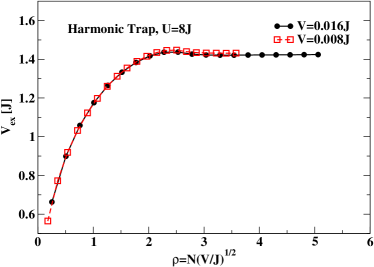
Figure 10: (Color online) Harmonic trap: Expansion velocity for $V=0.008J$ and $V=0.016J$ as a function of effective density $\rho=N\cdot\sqrt{V/J}$ for $U=8J$. The expansion velocity is remarkably stable against changing the particle number at fixed $\rho$.

Appendix B: Finite-size effects

Here we address the question of how our results for the expansion velocity depend on the overall particle number at a fixed density $n_{\mathrm{init}}$. First, we consider the box trap and we compare our analytical result for large $N$ [Eq. (3)] to exact diagonalization in the noninteracting limits in Fig. 8. For $N=40$, we find good qualitative agreement with small finite-size effects, which are the most pronounced for $n_{\mathrm{init}}<0.5$. For $N=160$, the deviations between the analytical expression for $N\to\infty$ and data for a finite $N$ are already barely visible except for very low densities. Second, we study the interacting system expanding from different box traps with $L_{\mathrm{init}}=10,20,40$ at a fixed density for $U=8J$. Figure 9 shows $V_{\mathrm{ex}}$ as a function of density. As in the non-interacting case finite-size effects are remarkably small whenever $n_{\mathrm{init}}\geq 0.6$ even for the smaller particle numbers. Finally, we turn to the expansion from a harmonic trap and analyze $V_{\mathrm{ex}}$ for two different trapping potentials, $V=0.008J$ and $V=0.016J$. Fig. 10 shows $V_{\mathrm{ex}}$ as a function of effective density $\rho=N\sqrt{V/J}$. We find that the expansion velocity is very robust against changing the particle number at a fixed $\rho$. Overall, our results for the expansion velocity exhibit only minor finite-size effects in all studied cases.

References

- (1) M. Rigol, V. Dunjko, and M. Olshanii, Nature (London) 452, 854 (2008).
- (2) A. Polkovnikov, K. Sengupta, A. Silva, and M. Vengalattore, Rev. Mod. Phys 83, 863 (2011).
- (3) I. Bloch, J. Dalibard, and W. Zwerger, Rev. Mod. Phys. 80, 885 (2008).
- (4) M. Rigol and A. Muramatsu, Phys. Rev. Lett. 93, 230404 (2004).
- (5) M. Rigol and A. Muramatsu, Phys. Rev. Lett. 94, 240403 (2005).
- (6) A. Rosch, D. Rasch, B. Binz, and M. Vojta, Phys. Rev. Lett. 101, 265301 (2008).
- (7) S. Mandt, A. Rapp, and A. Rosch, Phys. Rev. Lett. 106, 250602 (2011).
- (8) F. Heidrich-Meisner, M. Rigol, A. Muramatsu, A. E. Feiguin, and E. Dagotto, Phys. Rev. A 78, 013620 (2008).
- (9) F. Heidrich-Meisner, S. R. Manmana, M. Rigol, A. Muramatsu, A. E. Feiguin, and E. Dagotto, Phys. Rev. A 80, 041603(R) (2009).
- (10) For bosons see: D. Muth, D. Petrosyan and M. Fleischhauer Phys. Rev. A 85, 013615 (2012)
- (11) I. Hen and M. Rigol, Phys. Rev. Lett. 105, 180401 (2010).
- (12) M. Jreissaty, J. Carrasquilla, F. A. Wolf, and M. Rigol, Phys. Rev. A 84, 043610 (2011).
- (13) E. Lundh, Phys. Rev. A 84, 033603 (2011)
- (14) A. del Campo and J. G. Muga, Europhys. Lett. 74, 965 (2006)
- (15) A. del Campo, Phys. Rev. A 78, 045602 (2008)
- (16) T. Kinoshita, T. Wenger, and S. D. Weiss, Nature (London) 440, 900 (2006).
- (17) U. Schneider, L. Hackermüller, J. P. Ronzheimer, S. Will, S. Braun, T. Best, I. Bloch, E. Demler, S. Mandt, D. Rasch, and A. Rosch, Nature Phys. 8, 213 (2012).
- (18) P. Medley, D. M. Weld, H. Miyake, D. E. Pritchard, and W. Ketterle, Phys. Rev. Lett. 106, 195301 (2011).
- (19) J. A. Joseph, J. E. Thomas, M. Kulkarni, and A. G. Abanov, Phys. Rev. Lett. 106, 150401 (2011).
- (20) T. Anker, M. Albiez, R. Gati, S. Hunsmann, B. Eiermann, A. Trombettoni, and M. K. Oberthaler, Phys. Rev. Lett. 94, 020403 (2005).
- (21) A. Sommer, M. Ku, G. Roati, and M. W. Zwierlein, Nature (London) 472, 102 (2011).
- (22) U. Schneider, L. Hackermüller, S. Will, T. Best, I. Bloch, T. A. Costi, R. W. Helmes, D. Rasch, and A. Rosch, Science 322, 1520 (2008).
- (23) R. Jördens, N. Strohmaier, K. Günter, H. Moritz, and T. Esslinger, Nature (London) 455, 204 (2008).
- (24) X. Zotos, F. Naef, and P. Prelovšek, Phys. Rev. B 55, 11029 (1997).
- (25) See, e.g., F. Heidrich-Meisner, A. Honecker, W. Brenig, Eur. Phys. J Spec. Topics 151, 135 (2007); C. Karrasch, J. H. Bardarson, J. E. Moore, arXiv:1111.4508, and further references cited therein.
- (26) A. Rosch and N. Andrei Phys. Rev. Lett. 85, 1092 (2000).
- (27) T. Prosen, Phys. Rev. Lett. 106, 217206 (2011).
- (28) A. Daley, C. Kollath, U. Schollwöck, and G. Vidal, J. Stat. Mech.: Theory Exp. (2004), P04005.
- (29) S. R. White and A. E. Feiguin, Phys. Rev. Lett. 93, 076401 (2004).
- (30) U. Schollwöck, Ann. Phys. (NY) 326, 96 (2011).
- (31) U. Schollwöck, Rev. Mod. Phys. 77, 259 (2005).
- (32) K. Rodriguez, S. Manmana, M. Rigol, R. Noack, and A. Muramatsu, New J. Phys. 8, 169 (2006).
- (33) A. Minguzzi and D. M. Gangardt, Phys. Rev. Lett. 94, 240404 (2005).
- (34) V. Gritsev, P. Barmettler, and E. Demler, New J.Phys. 12, 113005 (2010).
- (35) D. Karlsson, C. Verdozzi, M. Odashima, and K. Capelle, EPL 93, 23003 (2011).
- (36) J. Kajala, F. Massel, and P. Törmä, Phys. Rev. Lett. 106, 206401 (2011).
- (37) J. Kajala, F. Massel, and P. Törmä, Phys. Rev. A 84, 041601(R) (2011).
- (38) M. Rigol and A. Muramatsu, Phys. Rev. A 69, 053612 (2004).
- (39) T. Park and J. Light, J. Chem. Phys 85, 5870 (1986).
- (40) M. Hochbruck and C. Lubich, SIAM J. Numer. Anal. 34, 1911 (1997).
- (41) A. Ashkin, PNAS 17, 12108 (2004).
- (42) T.P. Meyrath, F. Schreck, J.L. Hanssen, C.-S. Chuu, and M.G. Raizen, Phys. Rev. A, 71, 041604(R) (2005).
- (43) M. Polini and G. Vignale, Phys. Rev. Lett. 98, 266403 (2007).
- (44) S. Langer, F. Heidrich-Meisner, J. Gemmer, I.P. McCulloch, and U. Schollwöck, Phys. Rev. B 79, 214409 (2009).
- (45) S. Langer, M. Heyl, I.P. McCulloch, and F. Heidrich-Meisner, Phys. Rev. B 84, 205115 (2011).
- (46) T. Giamarchi, Quantum Physics in One Dimension, Clarendon Press, Oxford, 2004.
- (47) A. Rosch, private communication.
- (48) The one dimensional case is discussed in the eprint version arXiv:1005.3545v1 of schneider11
- (49) J. L. Vázquez, Smoothing and Decay Estimates for Nonlinear Diffusion Equations (Oxford University Press, Oxford, 2006)