The oscillating two-cluster chimera state in non-locally coupled phase oscillators

Abstract

We investigate an array of identical phase oscillators non-locally coupled without time delay, and find that chimera state with two coherent clusters exists which is only reported in delay-coupled systems previously. Moreover, we find that the chimera state is not stationary for any finite number of oscillators. The existence of the two-cluster chimera state and its time-dependent behaviors for finite number of oscillators are confirmed by the theoretical analysis based on the self-consistency treatment and the Ott-Antonsen ansatz.

1 Introduction

An array of identical oscillators has been used to model a wide range of systems, such as neural networks, convecting fluids, laser arrays and coupled biochemical oscillators. These systems exhibit rich collective behaviors including synchrony and spatiotemporal chaos [1, 2, 3, 4]. Most of the earlier theoretical works on these systems assume either local coupling (nearest-neighbor interactions) or global coupling (infinite-range interactions); a third type named non-locally coupling began to be explored in the past years, which is somewhere between local coupling and global coupling. In non-local coupled systems, the oscillators interact with all others and the strength between oscillators varies with the distance between them.

Chimera state is a spatiotemporal pattern in which some of the identical oscillators are coherent and synchronous while others remain incoherent [5, 6, 7, 8, 9]. They usually appear in systems with non-local coupling and could only be built for proper initial conditions [10]. Chimera state does not relate to the partially synchronized states observed in populations of nonidentical oscillators with dispersive frequencies in which the splitting of the population roots in the inhomogeneity of the oscillator themselves and the intrinsically fastest or slowest oscillators remain desynchronized. Its emergence cannot be ascribed to a supercritical instability of the spatially uniform oscillation, because it occurs even if the uniform state is stable. Chimera may be a paradigm to study unihemispheric sleep in neurology which states a fact that many creatures sleep with only half of their brain while the other half is still active at the same time. [11].

In the year 2002, Chimera state was first reported by Kuramoto and his colleagues [5, 6] when simulating the non-locally coupled complex Ginzburg-Landau equation. They showed that identical oscillators with non-locally symmetrical coupling could self-organize into chimera states. Soon, spiral wave chimera [12, 13] was discovered in two-dimensional arrays of non-locally coupled oscillators. In succession, Abrams and Strogatz [7] found an exact solution for this state in a ring of phase oscillators coupled by a cosine kernel. Recently, two interesting findings on chimera state are reported. Firstly, in the study of the non-locally coupled oscillators with time delay [14, 15], clustered chimera state that has spatially distributed phase coherence separated by incoherence with adjacent coherent regions in antiphase, was found. The observed clustered chimera state in these systems is stationary and its pattern does not change with time. Secondly, Abrams and Strogatz [16] found a breathing chimera state in a model consisting of two interacting subpopulations of oscillators. Pikovsky and Rosenblum [17] considered oscillators ensembles consisting of several subpopulations of identical units, with a general heterogeneous coupling between subpopulations, through which they acquired quasiperiodic chimera states. Laing [18, 19] summarized chimera states in several heterogeneous networks of coupled phase oscillators, in the mean time, he analyzed chimera state applying the Ott-Antonsen ansatz [20] in one-dimensional and two-dimensional systems. He pointed out that, in one-dimensional system, when parameter heterogeneity is introduced, a breathing chimera state exists.

In this work, we study a one-dimensional array of non-locally coupled identical phase oscillators. We find that, in the absence of time delay, a two-cluster chimera state could exist. We also find that, in the absence of parameter heterogeneity, the two-cluster chimera state is not stationary but oscillating. Different from Laing’s results [20], we find that the oscillation of the two-cluster chimera state only exists for the system with a finite number of oscillators. Both the two-clustered chimera state and finite size oscillations of the chimera state in this model are analyzed based on the Ott-Antonsen ansatz.

2 Model

The array of non-locally coupled phase oscillators can be described in a concise form as

$$\frac{\partial\phi}{\partial t}=\omega-\int_{-k}^{k}G(x-x^{\prime})\sin[\phi(x,t)-\phi(x^{\prime},t)+\alpha]dx^{\prime}.$$ (1)

Here, $\phi(x,t)$ is the phase of the oscillator at position $x$ at time $t$. The space variable $x$ is in the range $[-k,k]$ $(0<k\leq\pi)$. The periodic boundary condition is imposed for $k=\pi$, otherwise the no-flux boundary condition is imposed on the system. $\omega$ is the natural frequency (same for all oscillators), which plays no role in the dynamics. Without losing generality, we can set $\omega=0$. The angle $\alpha$ $(0\leq\alpha\leq\frac{\pi}{2})$ is a tunable parameter. The kernel $G(x-x^{\prime})$ provides non-local coupling between oscillators. $G(x)$ is non-negative, even, decreasing with $|x|$ along the array, and normalized to have unit integral. Following Abrams and Strogatz [7], we make use of the cosine kernel

$$G(x)=\frac{1}{2(k+A\sin k)}(1+A\cos x)$$ (2)

where $0\leq A\leq 1$. When $k=\pi$, Abrams and Strogatz found a chimera state with only one coherent cluster [7]. However, we find a novel chimera state which has two coherent clusters and is oscillating for any finite number of oscillators. As mentioned above, clustered chimera state is only found in the time-delay coupled systems [14, 15] and oscillating chimera state is found in the systems with subpopulations [16, 17] or the systems with parameter heterogeneity [i.e., $\alpha=\alpha(x)$] [18].

Let $\Omega$ denotes the angular frequency of a rotating frame whose dynamics are simplified as much as possible, and let $\theta=\phi-\Omega t$ denotes the phase of an oscillator relative to this frame. The key idea behind the analysis of chimera stats is the introduction of a mean-field-like quantity, namely, a complex order parameter $Re^{i\Theta}$ [5, 6, 7] which is defined as

$$R(x,t)e^{i\Theta(x,t)}=\int_{-k}^{k}G(x-x^{\prime})e^{i\theta(x^{\prime},t)}dx^{\prime}$$ (3)

Then Eq (1) becomes

$$\frac{\partial\theta}{\partial t}=\omega-\Omega-R\sin(\theta-\Theta+\alpha).$$ (4)

For stationary state, $R$ and $\Theta$ are time-independent and only depend on space variable $x$. Let $\Delta=\omega-\Omega$ where $\Omega$ is the angular velocity for the oscillators in coherent regions, the oscillators with $\Delta\leq R$ are in coherent regions and are phase-locked to $\theta=\arcsin(\frac{\Delta}{R})+\Theta-\alpha$ [5, 6, 7].

3 Simulate and results

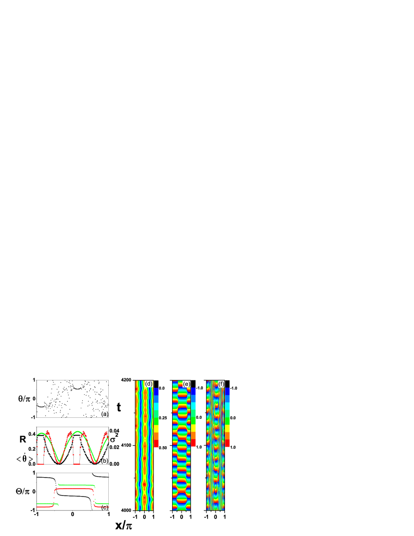
Figure 1: (color online) (a) Phase pattern for two-cluster chimera state when the steady state is reached. Eq. (1) is integrated using the Runge-Kutta method with fixed time step $dt=0.1$ with oscillator number $N=256$, $k=\pi$, $\beta=0.10$ and $A=0.995$. (b) The triangle (green) symbol is the modulus $R$ of the complex order parameter, the square (black) symbol is the distribution of $\langle\dot{\theta}(x)\rangle$ of individual oscillators averaged over 200 time units. The circle (red) symbol is the fluctuation $\sigma^{2}(x)$ of $\dot{\theta}(x)$. (c) three types of distribution of the phase $\Theta$ of the order parameter at different time. (d), (e) and (f) show the contour graphs of $R(x)$, $\Theta(x)/\pi$ and $\theta(x)/\pi$, respectively. The horizontal axis is position $x$ and vertical axis is time $t$.

For parameters $\beta=\frac{\pi}{2}-\alpha=0.10$, $A=0.995$, $k=\pi$, the system with $N=256$ phase oscillators could evolve to a two-cluster chimera state under the initial conditions as follows:

$$\phi(x,0)=\left\{\begin{array}[]{l l}2\pi re^{-2.76x^{2}},&x\leq 0\\ 2\pi re^{-2.76x^{2}}+\pi,&x>0\end{array}\right.$$ (7)

where $r$ is a random variable from a uniform distribution of $[-0.5,0.5]$. As shown in Fig. 1(a), there exist two coherent clusters in which all oscillators are synchronized. Oscillators in the same cluster are nearly in phase yet in different clusters are in antiphase. On the other hand, the oscillators between the two coherent clusters are de-synchronized and their phases are randomly distributed in $[-\pi,\pi]$.

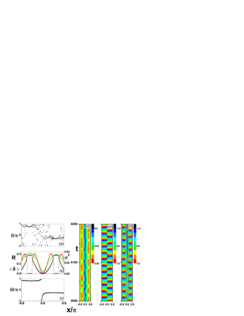
Figure 2: (color online) (a) Phase pattern for two-cluster chimera. The parameters $N=256$, $k=0.8\pi$, $\beta=0.10$ and $A=0.995$. (b) The triangle (green) symbol is the modulus $R$ of the complex order parameter, the square (black) symbol is the distribution of $\langle\dot{\theta}(x)\rangle$ of individual oscillators averaged over 200 time units. The circle (red) symbol is the fluctuation $\sigma^{2}$ of $\dot{\theta}(x)$. (c) the distribution of the phase $\Theta$ of order parameter. (d), (e) and (f) show the contour graphs of $R(x)$, $\Theta(x)/\pi$ and $\theta(x)/\pi$, respectively.

Then we consider three quantities characterizing a chimera state: the modulus $R$ of the complex order parameter at an arbitrary time, the angular velocity $\langle\dot{\theta}(x)\rangle$ averaged in a time interval of 200 units, and the fluctuation of the instantaneous angular velocity which is defined as $\sigma(x)=\sqrt{\langle(\dot{\theta}(x)-\langle\dot{\theta}(x)\rangle)^{2}\rangle}$. The quantities against the locations of oscillators are presented in Fig. 1(b). Clearly, there are two plateaus on the curve of $\langle\dot{\theta}(x)\rangle$ which refer to the coherent clusters in the chimera state. The zero $\sigma$ in the coherent clusters means that the oscillators in the coherent clusters all move on the same instantaneous angular velocity. Further, nonzero $\sigma$ outside the coherent clusters refers to the fluctuation of angular velocities for the oscillators outside the coherent clusters and indicates desynchronization. Fig. 1(b) reveals two features on $R$ for the two-cluster chimera state. Firstly, the oscillators can be divided into two domains which join at the minimum of $R$ and the curve of $R$ against the locations of oscillators does not show symmetry about the minimum of $R$. Further explorations show that $R$ is a function of time. As shown in Fig. 1(d) where the spatiotemporal evolution of $R$ is featured, $R$ is oscillating in each coherent cluster. Especially, when $R$ reaches its minimum in one domain, $R$ in the other one reaches its maximum. Secondly, the boundaries of the coherent clusters are not determined by the condition of $\Delta=R(x)$ and the coherent regimes are narrower than those expected according to $\Delta=R(x)$ in most of the time, which are different from the stationary chimera state. The reason for this observation roots in the time-dependent order parameter $R$. Actually, for a forced phase oscillator obeying $\dot{\theta}=\omega+R(t)\sin\theta$, the synchronization of the phase oscillator by the force just requires the phase of the oscillator to be confined within $(0,2\pi)$ but not to a fixed value, which leads the onset of the synchronization of the oscillator not to obey the condition of $\Delta=R(t)$ and the onset of synchronization strongly depends on the details of the functional form of $R(t)$. To be noted, even though $R$ is time-dependent, the oscillators in the coherent clusters still have the same angular velocity which does not fluctuate as exhibited by zero $\sigma$. The spatiotemporal evolution of $R$ in Fig. 1(d) shows another feature: the two-cluster chimera state displays an irregular motion along the ring, for example, the locations of coherent clusters vary with time. Similar phenomenon is also observed for the chimera state with a single cluster [21]. Furthermore, the snapshot and the time evolution of $\Theta$ presented in Fig. 1(c) and (e) show that $\Theta$ is almost uniform in each domain except for those near the junction between domains and there is a phase difference of $\pi$ for $\Theta$ in different domains. To be stressed, the features on $\Theta$ revealed by Fig. 1(c) and (e) could be used as a more general scheme for the initial conditions to generate an oscillating two-cluster chimera state. That is, the initial conditions in Eq. 7 could be changed to be $\phi(x,0)=\pi$ for $x\leq 0$ and $\phi(x,0)=0$ for $x>0$. To get a better illustration, we present the evolution of $\theta(x)$ in Fig. 1(f) which shows that, resulting from the oscillation of $R$, the territories of the coherent clusters alter with time. Furthermore, it should be pointed out that, though a two-cluster chimera state could be generated for the system characterized by Eq. 1 in the absence of time delay under proper initial conditions, we have not detected other chimera states with more than two coherent clusters.

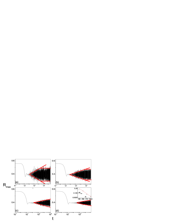
Figure 3: (color online) The maxima of $R$ in one domain varies with time for different number of oscillators. (a, b, c, d) are for $N=128$, $256$, $512$ and $1024$, respectively. Other parameters: $A=0.995$, $\beta=0.1$ and $k=0.8\pi$. The (red) lines denote the growth of $R$ in the transient and the upper or lower bound of the maxima of $R$ in the steady state. The inset in (d) shows the amplitude of the oscillation of $R_{max}$, $\Delta R_{max}$, against the system size $N$, which indicates a power law of $\Delta R_{max}\sim N^{-0.5}$.

The two-cluster oscillating chimera state can exist when $k\neq\pi$. In comparison with the case with $k=\pi$ where oscillators locate on a ring, here the oscillators locate on a chain. We take $k=0.8\pi$ as an example. The results are given in Fig. 2. The differences with those in Fig. 1 are that the pattern of two-cluster chimera state becomes stationary in space and, no matter where the chimera state is initialized, it will adjust its pattern to be symmetrical about the center of the chain where the minimum of $R$ appears.

The analysis above are made on the system with $N=256$. One question is how the observed two-cluster oscillating chimera state depends on the number of oscillators. For this aim, we focus on one domain and record the maximum value of $R$ in this domain at any time instance (we denote it as $R_{max}$). The time-dependent behavior of the two-cluster chimera state can be reflected by the time evolution of $R_{max}$. For example, a constant $R_{max}$ indicates a stationary chimera state, otherwise an oscillating one. To avoid the influences induced by the irregular motion of the chimera state along the ring in the system with periodic boundary condition, we let $k=0.8\pi$. The results for different $N$ are presented in Fig. 3. One remarkable feature revealed by the figure is that, before the oscillating chimera state is established, the system first evolves to a two-cluster chimera state which looks like a stationary one due to the weak oscillation of $R_{max}$. However, the ”stationary” state is not stable and its instability leads to the appearance of an oscillating chimera state. Interestingly, the stationary value of $R_{max}$ is independent of the size of the system and the time consumed for the system to build an oscillating state becomes much longer as the number of the oscillator $N$ increases. Another feature in Fig.3 is that larger $N$ seems to weaken the oscillation of $R_{max}$ in the two-cluster oscillating chimera state, which is prominent by the comparison between Fig. 3 (a) ($N=128$) and (b) ($N=256$). Since the transient time to build an oscillating two-cluster chimera state for large $N$ becomes extremely long, we just give a rough estimate based on the data presented in the inset of Fig. 3(d) that the oscillation amplitude $\Delta R_{max}\sim N^{-0.5}$, which means that the two-cluster oscillating chimera state becomes a stationary one in the thermodynamic limit, which is different from the Laing’s results [20].

4 Analysis

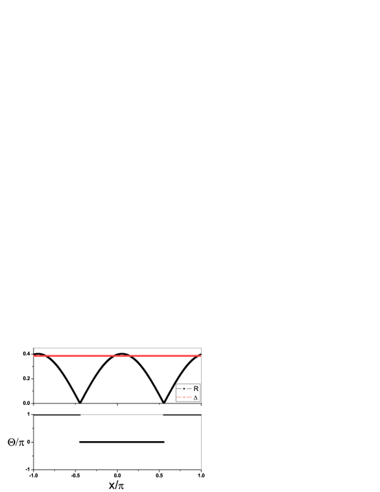
Figure 4: (color online) The modulus $R$ and the phase $\Theta$ of the order parameter and $\Delta$ by solving of Eq. (13) via an iterative scheme as presented in the context. (a) The square (black) symbol denotes the distribution of $R$ and the circle (red) the value of $\Delta$. (b) Distribution of $\Theta$. Other parameters: $A=0.995$, $\beta=0.1$ and $k=\pi$.

The above results can be understood theoretically. First, the two-cluster stationary chimera state in the thermodynamic limit can be explained in terms of Kuramoto-Battogtokh self-consistency equation[5] as follows:

$$R(x)e^{i\Theta(x)} = e^{i\beta}\int_{-\pi}^{\pi}G(x-x^{\prime})e^{i\Theta(x^{\prime})}\times\frac{\Delta-\sqrt{\Delta^{2}-R(x^{\prime})^{2}}}{R(x^{\prime})}dx^{\prime}$$ (8)

note that there are three unknown quantities (the real-valued functions $R(x)$, $\Theta(x)$ and the real number $\Delta$) in terms of the assumed choices of $\beta$ and the kernel $G(x-x^{\prime})$. We take $k=\pi$ as an example. Considering the patterns in Figs. 1(b) and (c), the modulus $R$ and the phase $\Theta$ of the order parameter approximately satisfy

$$\left\{\begin{array}[]{l l}R(x+\pi)=R(x)\\ \Theta(x+\pi)=\Theta(x)+\pi.\end{array}\right.$$ (11)

We substitute Eqs. (11) and (2) into Eq. (8) and get

$$R(x)e^{i\Theta(x)}=e^{i\beta}\int_{-\pi}^{0}\frac{1}{2\pi}[1+A\cos(x-x^{\prime})e^{i\Theta(x^{\prime})}H(x^{\prime})dx^{\prime}$$

$$+e^{i\beta}\int_{0}^{\pi}\frac{1}{2\pi}[1+A\cos(x-x^{\prime})]e^{i\Theta(x^{\prime})}H(x^{\prime})dx^{\prime},$$ (12)

where $H(x)=(\triangle-\sqrt{\Delta^{2}-R(x)^{2}})/R(x)$. Under the transformation $x^{\prime}-\pi\rightarrow x^{\prime}$ in the second term of the right hand side of Eq. (12), the self-consistency equation changes into

$$R(x)e^{i\Theta(x)}=e^{i\beta}\int_{-\pi}^{0}\frac{A\cos(x-x^{\prime})}{\pi}e^{i\Theta(x^{\prime})}H(x^{\prime})dx^{\prime}.$$ (13)

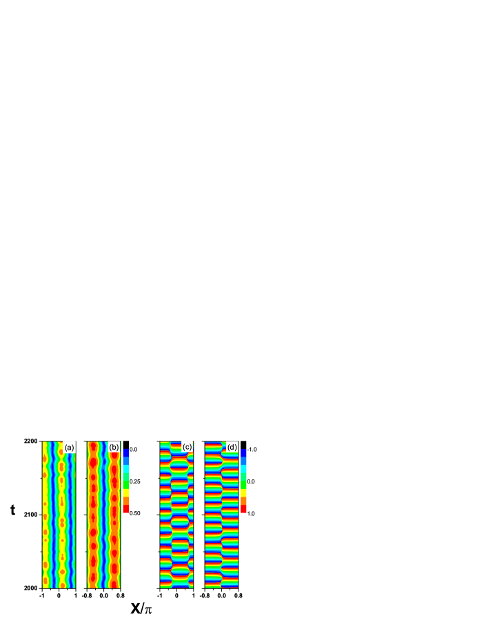
Figure 5: (color online) Phase pattern for two-cluster chimera when the steady state is reached. Eq. (21) and (22) is integrated using the Runge-Kutta method with fixed time step $dt=0.005$ and the oscillator number $N=256$. (a, c) are the modulus $R$ and the phase $\Theta/\pi$ of the complex order parameter with $k=\pi$. (b, d) are the modulus $R$ and the phase $\Theta/\pi$ of the complex order parameter with $k=0.8\pi$. Other parameters: $\beta=0.1$, $A=0.995$.

To solve Eq. (13), we first determinate the value of $\Delta$. Because Eq. (13) is left unchanged by any rigid rotation $\Theta(x)\rightarrow\Theta(x)+\Theta_{0}$, we can specify the value of $\Theta(x)$ at any point $x$ we like. We set $\Theta(\frac{\pi}{2})=0$. Now we can get $\Delta$. Then we take $R(x)$ and $\Theta(x)$ obtained from the dynamical simulations as initial guesses and use an iterative scheme to determinate $R(x)$ and $\Theta(x)$ in function space, behind which the idea is that the current estimates of $R(x)$ and $\Theta(x)$ can be entered into the right-hand side of (13), and used to generate the new estimates appearing on the left-hand side. Figure 4 shows the results obtained from Eqs.(9) and (2). To be stressed, without the requirement of Eq.(7), the self-consistency equation for any finite system always yields to a one-cluster chimera state, which also evidences that the stationary two-cluster chimera state here is not stable.

From Fig. 4, we could notice the order parameter of stationary state, which has a little difference from Fig. 1(b) and (c) in the vicinity of the junction between two domains. The transition of the former case performances like a step function while the latter one is continuous. The difference probably originates from the finite size effect in Fig. 1.

The oscillating characteristic could be interpreted with the assistance of the Ott-Antonsen ansatz [18, 20]. Following the line in [16, 17, 18], we assume that there is a probability density function $f(x,\omega,\theta,t)$ characterizing the state of the system. This function satisfies the continuity equation [16, 17, 18, 19]

$$\frac{\partial f}{\partial t}+\frac{\partial}{\partial\theta}(fv)=0$$ (14)

where

$$v=\omega-\int_{-k}^{k}G(x-x^{\prime})\int_{-\infty}^{\infty}\int_{-\pi}^{\pi}\sin(\theta-\theta^{\prime}+\alpha)f(x^{\prime},\omega,\theta^{\prime},t)d\theta^{\prime}d\omega dx^{\prime}$$ (15)

with $\theta=\theta(x)$ and $\theta^{\prime}=\theta(x^{\prime})$. The complex order parameter can be formulated as

$$Z\equiv Re^{i\Theta}=\int_{-k}^{k}G(x-x^{\prime})\int_{-\infty}^{\infty}\int_{-\pi}^{\pi}e^{i\theta^{\prime}}f(x^{\prime},\omega,\theta^{\prime},t)d\theta^{\prime}d\omega dx^{\prime}.$$ (16)

In terms of complex order parameter $Z$, Eq. (15) can be rewritten as

$$v=\omega-\frac{1}{2}[Ze^{-i(\theta-\beta)}+Z^{*}e^{i(\theta-\beta)}]$$ (17)

where $Z^{*}$ denotes the complex conjugate of $Z$ and $\beta=\frac{\pi}{2}-\alpha$. Following Ott and Antonsen [18, 20], we have

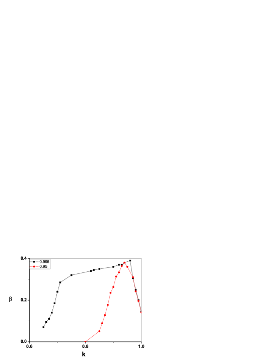
Figure 6: (color online) The boundary of the two-cluster chimera state plotted on $k-\beta$ parameter plane. Below the curves, the two-cluster chimera state is stable. The square (black) symbol and circle (red) symbol are plotted at the parameter values $A=0.995$ and $A=0.95$, respectively.

$$f(x,\omega,\theta,t)=\frac{g(\omega)}{2\pi}\{1+\sum_{n=1}^{\infty}[(a(x,\omega,t)e^{i\theta})^{n}+c.c.]\}$$ (18)

where $c.c.$ is the complex conjugate of the previous term and $g(\omega)$ is the distribution of natural frequency. In this work, we assign all oscillators a same natural frequency ($\omega=0$), so $g(\omega)=\delta(\omega)$. Substituting Eqs.(17) and (18) into Eqs. (14) and (16), we obtain

$$\frac{\partial a(x,\omega,t)}{\partial t}=\frac{i}{2}[Z^{*}e^{-i\beta}+Ze^{i\beta}a^{2}]$$ (19)

$$Z=\int_{-k}^{k}G(x-x^{\prime})\int_{-\infty}^{\infty}g(\omega)a^{*}(x,\omega,t)d\omega dx^{\prime}.$$ (20)

Letting $\hat{a}(x,t)=a(x,0,t)$, we have

$$\frac{\partial\hat{a}(x,t)}{\partial t}=\frac{i}{2}[Z^{*}e^{-i\beta}+Ze^{i\beta}\hat{a}^{2}]$$ (21)

$$Z=\int_{-k}^{k}G(x-x^{\prime})\hat{a}^{*}(x^{\prime},t)dx^{\prime}.$$ (22)

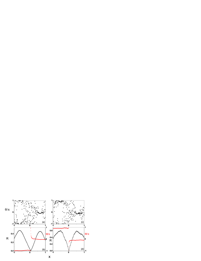
Figure 7: (color online) Two-cluster chimera under the condition of different types of nonlocal coupling kernel $G(x)$. The top panels are the phase patterns for two-cluster chimera and the bottom are the modulus $R$ (black) and the phase $\Theta$ (red) of the order parameters. (a, b) is computed under the assumption that $G(x)$ takes exponential form with parameters: $A=4$, $k=1$ and $\beta=0.10$ while $G(x)$ in (c, d) is steplike function with parameters: $d=0.5$, $k=1$ and $\beta=0.10$. All above take no-flux boundary condition and the initial conditions are as following: $\phi(x,0)=0$ for $x<0$ and $\phi(x,0)=\pi$ for $x>0$

By numerically simulating these two equations, we have the time evolutions of $R(x)$ and $\Theta(x)$. The results for $k=\pi$ and $k=0.8\pi$ are presented in Fig. 5, respectively. Clearly, the main features in Figs. (1) and (2), such as the oscillating nature of the two-cluster chimera state, the movement of the pattern (or the frozen pattern) of $R$ and $\Theta$ for $k=\pi$ (or for $k=0.8\pi$), and the uniform distribution of $\Theta(x)$ in different domains, are reproduced in Fig. 5.

Using Eqs. (21) and (22), we may probe into the regime for the existence of the two-cluster chimera state on $k-\beta$ parameter plane. The results are presented in Fig. 6 at $A=0.995$ and $A=0.95$. As shown in this plot, the two-cluster chimera state is not favorable at large $\beta$, and either small $k$ or large $k$ tends to be harmful for the two-cluster chimera state. And the smaller $A$ is, the smaller the domain of two-clustered chimera exists. if $A<0.8$, the domain does not exist any longer. Beyond the stable regime for the two-cluster chimera, i.e., above the curves in Fig. 6, the initial two-cluster chimera state tends to become a normal chimera state with only one coherent cluster. The two-cluster oscillating chimera state may be detected in coupled oscillators with other types of non-locally coupling kernel $G(x)$ which could be exemplified by two cases. In the first one, $G(x)$ takes an exponentially decaying function, $G_{exp}(x)=\frac{Ae^{-A|x|}}{2(1-e^{-Ak})}$. In the other case, $G(x)$ takes a steplike function, $G_{step}(x,d)=\frac{1}{2d}$ for $|x|\leq d$ and $G_{step}(x,d)=0$ for $|x|>d$. Figure 7 shows the results for the systems with these two types of non-locally coupling and, clearly, the two-cluster oscillating chimera states are reproduced.

5 Conclusion

In summary, we study a one-dimensional system consisting of non-locally coupled phase oscillators, which is a prototype for studying chimera states. By numerically simulating this simplest system, we find the existence of a two-cluster oscillating chimera state in the absence of time delay coupling and parameter heterogeneity. The numerical results are confirmed by the theoretical analysis based on the self-consistency treatment and the Ott-Antonsen ansatz.

References

References

- [1] Y. Braiman, J. F. Lindener and W. L. Ditto, Nature 378, 465 (1995).
- [2] L. Kocarev and U. Parlitz, Phys. Rev. Lett. 77, 2206 (1996).
- [3] H. G. Winful and L. Rahman, Phys. Rev. Lett. 65, 1575 (1990).
- [4] L. Kocarev, U. Parlitz, T. Stojanovski and P. Janjic, Phys. Rev. E 56, 1238 (1997).
- [5] Y. Kuramoto and D. Battogtkh, Nonlinear Phenomena in Complex Systems 5, 380 (2002).
- [6] D. Tanaka and Y. Kuramoto, Phys. Rev. E 68, 026219 (2003).
- [7] D. M. Abrams and S. H. Strogatz, Phys. Rev. Lett. 93, 174102 (2004).
- [8] Y. Kawamura, Phys. Rev. E 75, 056204 (2007).
- [9] O. E. Omel’chenko, Y. L. Maistrenko and P. A. Tass, Phys. Rev. Lett. 100, 044105 (2008).
- [10] A. E. Motter, Nat. Phys. 6, 164 (2010)
- [11] C. G. Mathews, J. A. Lesku, S. L. Lima, and C. J. Amlaner, Ethology 112, 286 (2006).
- [12] S. I. Shima and Y. Kuramoto, Phys. Rev. E 69, 036213 (2004).
- [13] E. A. Martens, C. R. Laing and S. H. Strogatz, Phys. Rev. Lett. 104, 044101 (2010).
- [14] J. H. Sheeba, V. K. Chandrasekar and M. Lakshmanan, Phys. Rev. E 81, 046203 (2010).
- [15] G. C. Sethia, A. Sen and F. M. Atay, Phys. Rev. Lett. 100, 144102 (2008).
- [16] D. M. Abrams, R. Mirollo, S. H. Strogatz and D. A. Wiley, Phys. Rev. Lett. 101, 084103 (2008).
- [17] A. Pikovsky and M. Rosenblum, Phys. Rev. Lett. 101, 264103 (2008).
- [18] C. R. Laing, Physica D 238, 1569 (2009).
- [19] C. R. Laing, Chaos 19, 013113 (2009).
- [20] E. Ott and T. M. Antonsen, Chaos 18, 037113 (2009).
- [21] O. E. Omel’chenko, M. Wolfrum, and Y. L. Maistrenko, Phys. Rev. E 81, 065201 (2010).