Inhomogeneity-induced variance of cosmological parameters

Abstract

Modern cosmology relies on the assumption of large-scale isotropy and homogeneity of the Universe. However, locally the Universe is inhomogeneous and anisotropic. This raises the question of how local measurements (at the $\sim 10^{2}$ Mpc scale) can be used to determine the global cosmological parameters (defined at the $\sim 10^{4}$ Mpc scale)? We connect the questions of cosmological backreaction, cosmic averaging and the estimation of cosmological parameters and show how they relate to the problem of cosmic variance. We used Buchert’s averaging formalism and determined a set of locally averaged cosmological parameters in the context of the flat $\Lambda$ cold dark matter model. We calculated their ensemble means (i.e. their global value) and variances (i.e. their cosmic variance). We applied our results to typical survey geometries and focused on the study of the effects of local fluctuations of the curvature parameter. We show that in the context of standard cosmology at large scales (larger than the homogeneity scale and in the linear regime), the question of cosmological backreaction and averaging can be reformulated as the question of cosmic variance. The cosmic variance is found to be highest in the curvature parameter. We propose to use the observed variance of cosmological parameters to measure the growth factor. Cosmological backreaction and averaging are real effects that have been measured already for a long time, e.g. by the fluctuations of the matter density contrast averaged over spheres of a certain radius. Backreaction and averaging effects from scales in the linear regime, as considered in this work, are shown to be important for the precise measurement of cosmological parameters.

1 Introduction

How do inhomogeneities in the matter distribution of the Universe affect our conception of its expansion history and our ability to measure cosmological parameters? Typically, these measurements rely on the averaging of a large number of individual observations. In an idealised situation we can think of them as volume averages. To give an example, the power spectrum, which is the Fourier–transformed two–point correlation function, may be seen as a volume average with weight $e^{ikx}$. Measurements of the properties of the large–scale structure rely on the observation of large volumes that have been pushed forward to ever higher redshifts in the last decade, from the two–degree Field survey (2dF, Colless et al. 2001) over the Sloan Digital Sky Survey (SDSS, Abazajian et al. 2009) to the current WiggleZ (Drinkwater et al., 2010) and Baryon Oscillation Spectroscopic Survey (BOSS, Eisenstein et al. 2011).

A theorem by Buchert states that the evolution of any volume-averaged comoving domain of an arbitrary irrotational dust Universe may be described by the equations of a Friedmann–Lemaître–Robertson–Walker (FLRW) model, but driven by effective sources that encode inhomogeneities (Buchert, 2000, 2001). The consequences of this have been studied extensively in perturbation theory (Kolb et al., 2005; Li & Schwarz, 2007, 2008; Brown et al., 2009a, b; Larena, 2009; Clarkson et al., 2009; Buchert et al., 2011) and for non-perturbative models (Buchert et al., 2006; Marra et al., 2007; Räsänen, 2008; Kainulainen & Marra, 2009; Roy & Buchert, 2010). Apart from the ongoing debate to what extent the global evolution is modified through backreaction effects from small-scale inhomogeneities (Räsänen, 2004; Ishibashi & Wald, 2006; Kolb et al., 2006; Buchert, 2008; Buchert et al., 2009; Wiegand & Buchert, 2010), Li & Schwarz (2008) showed that the measurement of cosmological parameters is limited by uncertainties concerning the relation between observable locally and unobservable globally averaged quantities.

In contrast to the well–studied cosmic variance of the cosmic microwave background, which is most relevant at the largest angular scales, the theoretical limitation on our ability to predict observations at low redshift arises not only from the fact that we observe only one Universe, but also from the fact that we sample a finite domain (much smaller than the Hubble volume). Both limitations contribute to the cosmic variance. This is different from the sampling variance caused by shot noise, i.e. the limitation of the sampling of a particular domain because of the finite number of supernovae (SN) or galaxies observed. In the era of precision cosmology, the errors caused by cosmic variance may become a major component of the error budget.

The purpose of this work is to demonstrate that the questions of cosmic averaging, cosmological backreaction, and the problems of cosmic variance and parameter estimation are closely linked. We demonstrate that cosmic variance is actually one of the aspects of cosmological backreaction.

There have already been many studies on the effect of the local clumpiness on our ability to measure cosmological parameters. However, they focused mainly on the fluctuations in the matter density and on the variance of the Hubble rate. The former question has gained renewed interest in view of deep redshift surveys such as GOODS (Giavalisco et al., 2004), GEMS (Rix et al., 2004) or COSMOS (Scoville et al., 2007). Because the considered survey fields are small, the variance of the matter density is an important ingredient in the error budget and it has been found to be in the range of 20% and more, demonstrated empirically in SDSS data by Driver & Robotham (2010) and calculated numerically from linear perturbation theory in Moster et al. (2010).

The variance of the Hubble rate has been considered in the setup of this work, i.e. first order linear perturbation theory in comoving synchronous gauge, in Li & Schwarz (2008). A calculation of the same effect in Newtonian gauge has been performed in Clarkson et al. (2009) and Umeh et al. (2010); the two methods agree. Calculations of the fluctuations in the Hubble rate owing to peculiar velocities alone have a longer history (Kaiser, 1988; Turner et al., 1992; Shi et al., 1996; Wang et al., 1998). The effects of inhomogeneities on other cosmic parameters have been studied in Newtonian cosmology (Buchert & Ehlers, 1997; Buchert et al., 2000).

There has been less activity in studying the effects of the third important player besides number density and Hubble expansion: cosmic curvature. Even if the Universe is spatially flat, as expected by the scenario of cosmological inflation and consistent with the observations of the temperature anisotropies of the cosmic microwave background, the local curvature may be quite different. To answer the question how big this difference actually is for realistic survey volumes, we here extend the analysis of Li & Schwarz (2007, 2008), where these effects have been estimated for the first time. For the spatially flat Einstein-de Sitter (EdS) model, the averaged curvature parameter $\Omega_{\cal R}^{\cal D}$ has been shown to deviate from zero by $\sim 0.1$ on domains at the $100$ Mpc scale.

Here we adapt the analysis of Li & Schwarz (2008) to the case of a $\Lambda$CDM universe, introduce a more realistic power spectrum and use observationally interesting window functions, not restricted to full–sky measurements.

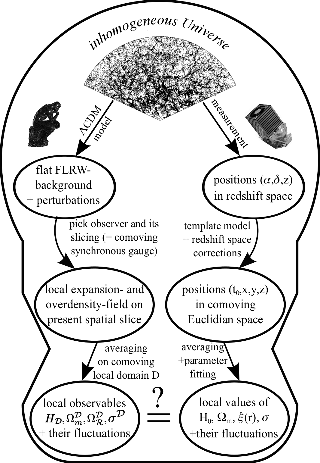
Figure 1: Comparison of the theorist’s and observer’s view on the Universe. Our calculation in comoving synchronous gauge facilitates the description of the boundaries of the experimentally investigated regions in our Universe. Note, that recently there have been attempts by Bonvin & Durrer (2011) to directly relate the two upper circles. This was done by calculating the predictions for the quantities in redshift space explicitly from the perturbed $\Lambda$CDM model.

There has been quite some confusion about the choice of gauge and the dependence of the averaged quantities on it. Recently it has been shown (Gasperini et al., 2010) that this is not a problem if one consistently works in one gauge and then expresses the quantity that is finally observed in this frame as well. This is easier in some gauges than in others, but the result is (as expected) the same, as is also confirmed explicitly by the fact that our results are consistent with those of Clarkson et al. (2009) and Umeh et al. (2010), obtained in Newtonian gauge. The quest for simplicity explains our choice to use comoving synchronous gauge, because this is the frame that is closest to the one used by the observers.

Fig. 1 depicts the theorist’s and the observer’s view on the Universe in a schematical way. It points out that in the end it is the average quantities that we are interested in, but that in an intermediate step, observers like to think of the objects they measure to lie in a comoving space with simple Euclidian distances. The comoving synchronous gauge, which has a clear notion of ”today” for a fluid observer sitting in a galaxy as we do, helps to define the things observers measure in a simple way.

In Section 2 we establish the conceptual framework for the study of effects of inhomogeneities on observable quantities. Section 3 and 4 generalize some of the results of Li & Schwarz (2007, 2008) and Li (2008) from an Einstein–de Sitter (EdS) to a $\Lambda$CDM background and implement a more realistic matter power spectrum. Section 5 investigates the effects of various window functions, again extending the analysis of Li & Schwarz (2008); Li (2008). Section 6 concentrates on deriving the magnitude of curvature fluctuations for realistic window functions. Section 7 applies the formalism to the local distance measure $D_{V}$, determined in the observation of baryonic acoustic oscillations (BAO). Section 8 is a remark on the link between the variance of averaged expansion rates at different epochs and the background evolution, before we conclude in Section 9.

2 Inhomogeneity and expansion

We assume that the overall evolution of the Universe is described by a flat $\Lambda$CDM model, which we adopt as our background model throughout this work. Global spatial flatness does not prevent the local curvature to deviate from zero.

The distribution of nearby galaxies indicates that the scales at which the Universe is inhomogeneous reach out to at least 100 Mpc. Above these scales it is not yet established if there is a turnover to homogeneity, as was claimed in Hogg et al. (2005), or if the correlations in the matter distribution merely become weaker, but persist up to larger scales, as is discussed in Labini (2010). At least morphologically, homogeneity has not been found up to scales of about 200 Mpc (Kerscher et al., 1998, 2001; Hikage et al., 2003).

Consequently, we need a formalism that is applicable in the presence of inhomogeneities at least for the description of the local expansion. This may be accomplished considering spatial domains ${\cal D}$ and averaging over their locally inhomogeneous observables (Buchert, 2000, 2001). Technically one performs a 3+1 split of spacetime. Because we considered pressureless matter only, we chose a comoving foliation in which the spatial hypersurfaces are orthogonal to the cosmic time. This means that the formalism will not be able to take into account lightcone effects. Therefore, it is well adapted for regions of the universe that are not too extended, a notion described more precisely in Sect. 5. The equations then describe the evolution of the volume of the domain ${\cal D}$, given by $\left|{\cal D}\right|_{g}:=\int_{{\cal D}}\,{\rm d}\mu_{g}$, where ${\rm d}\mu_{g}:=[{}^{(3)}g\left(t,{\mathbf{x}}\right)]^{1/2}{\rm d}^{3}x$ and ${}^{(3)}g$ is the fully inhomogeneous three–metric of a spatial slice.

To obtain an analogy to the standard Friedmann equations, one defines an average scale factor from this volume

$$a_{{\cal D}}\left(t\right):=\left(\frac{\left|{\cal D}\right|_{g}}{\left|{\cal D}_{0}\right|_{g}}\right)^{\frac{1}{3}}\;,$$ (1)

where the subindex $0$ denotes ”today”, as throughout the rest of this work. The definition implies $a_{{\cal D}_{0}}=1$. In analogy to the background model $H_{{\cal D}}:=\dot{a}_{{\cal D}}/a_{{\cal D}}$. The foliation may be used to define an average over a three–scalar observable $O$ on a domain ${\cal D}$ in the spatial hypersurface

$$\left\langle O\right\rangle_{\cal D}\left(t\right):=\frac{\int_{{\cal D}}\,O\left(t,{\mathbf{x}}\right){\rm d}\mu_{g}}{\int_{{\cal D}}\,{\rm d}\mu_{g}}.$$ (2)

Examples for these observables include the matter density $\varrho$ or the redshift $z$ of a group of galaxies in the domain ${\cal D}$.

The scalar parts of Einstein’s equations for an inhomogeneous matter source become evolution equations for the volume scale factor driven by quantities determined by this average:

$$3\frac{\ddot{a}_{{\cal D}}}{a_{{\cal D}}} = -4\pi G\left\langle\varrho\right\rangle_{\cal D}+{\cal Q}_{{\cal D}}+\Lambda,$$ (3)

$$3H_{{\cal D}}^{2} = 8\pi G\left\langle\varrho\right\rangle_{\cal D}-\frac{1}{2}\left\langle{\cal R}\right\rangle_{\cal D}-\frac{1}{2}{\cal Q}_{{\cal D}}+\Lambda,$$ (4)

$$0 = \partial_{t}\left\langle\varrho\right\rangle_{\cal D}+3H_{{\cal D}}\left\langle\varrho\right\rangle_{\cal D}.$$ (5)

The expansion of the domain ${\cal D}$ is determined by the average matter density, the cosmological constant, the average intrinsic scalar curvature $\left\langle{\cal R}\right\rangle_{\cal D}$ and the kinematical backreaction ${\cal Q}_{{\cal D}}$. The latter encodes the departure of the domain from a homogeneous distribution and is a linear combination of the variance of the expansion rate and the variance of the shear scalar.

Equations (3) to (5) mean that the local evolution of any inhomogeneous domain is described by a set of equations that corresponds to the Friedmann equations.

The cosmic parameters, defined by

$$\Omega_{m}^{{\cal D}} := \frac{8\pi G}{3H_{{\cal D}}^{2}}\left\langle\varrho\right\rangle_{\cal D},\quad\Omega_{\Lambda}^{{\cal D}}:=\frac{\Lambda}{3H_{{\cal D}}^{2}},$$ (6)

$$\Omega_{{\cal R}}^{{\cal D}} := -\frac{\left\langle{\cal R}\right\rangle_{\cal D}}{6H_{{\cal D}}^{2}},\quad\Omega_{{\cal Q}}^{{\cal D}}:=-\frac{{\cal Q}_{{\cal D}}}{6H_{{\cal D}}^{2}},$$

are domain–dependent. Owing to the fluctuating matter density, the curvature and the average local expansion rate will also fluctuate. When we constrain ourselves to the perturbative regime, the modification due to ${\cal Q}_{{\cal D}}$ is important on scales of the order of $10$ Mpc (Li & Schwarz, 2008).

Here we are interested to see to what extent the values of the parameters (6) vary if we look at different domains of size ${\cal D}$ in the Universe. We could therefore define an average over many equivalent domains ${\cal D}$ at different locations in our current spatial slice. For an ergodic process, however, this is the same as the variance of an ensemble average over many realizations of the Universe keeping the domain ${\cal D}$ fixed, but changing the initial conditions of the matter distribution. This is the quantity that we calculate in theory and therefore we have to rely on the assumption of ergodicity when comparing our results with the observation. In our case this ensemble average is taken over quantities that are volume averages. This means that for any observable $O$ there are two different averages involved. The domain averaging, $\left\langle O\right\rangle_{\cal D}$, and the ensemble average, $\overline{O}$. We assume that both averaging procedures commute.

The fluctuations are then characterized by the variance with respect to the ensemble averaging process,

$$\sigma\left(\left\langle O\right\rangle_{\cal D}\right):=\left(\overline{\left\langle O\right\rangle_{\cal D}^{2}}-\overline{\left\langle O\right\rangle_{\cal D}}^{2}\right)^{\frac{1}{2}}\;.$$ (7)

An example for a common observable calculated in this manner would be $\sigma_{8}$ as the ensemble r.m.s. fluctuation of the matter density field. To quantify these fluctuations of a general observable $O$, we use the theory of cosmological perturbations. In Li & Schwarz (2007) it has been shown that to linear order, the ${\cal Q}_{{\cal D}}$–term in equations (4) and (3) vanishes. $\left\langle\varrho\right\rangle_{\cal D}$, $\left\langle{\cal R}\right\rangle_{\cal D}$ and $H_{{\cal D}}$ however, have linear corrections.

Furthermore, Li (2008) argued that there is no second–order contribution to the fluctuations for Gaussian density perturbations if their linear contributions are finite. This may be seen by decomposing the observable $O$ into successive orders $O=O^{\left(0\right)}+O^{\left(1\right)}+O^{\left(2\right)}+\cdots$. It is usually assumed that $\overline{O^{(1)}}=0$. Now, for Gaussian perturbations only terms of even order give rise to non-trivial contributions. Therefore, (7) may be expressed as

$$\sigma\left(O\right)=\sqrt{\overline{\left(O^{\left(1\right)}\right)^{2}}}\left(1+\frac{\overline{\left(O^{\left(2\right)}\right)^{2}}-\left(\overline{O^{\left(2\right)}}\right)^{2}+2\overline{O^{\left(1\right)}O^{\left(3\right)}}}{2\overline{\left(O^{\left(1\right)}\right)^{2}}}\right),$$ (8)

which shows that the correction to the leading order linear term is already of third order. This is why we content ourselves for the evaluation of the fluctuations in the parameters $\left\langle\varrho\right\rangle_{\cal D}$, $\left\langle{\cal R}\right\rangle_{\cal D}$ and $H_{{\cal D}}$ or $\Omega_{m}^{{\cal D}}$, $\Omega_{{\cal R}}^{{\cal D}}$ and $H_{{\cal D}}$ to a first order treatment. This argument does not apply if $\overline{\left(O^{\left(1\right)}\right)^{2}}=0$, as is the case for ${\cal Q}_{\cal D}$. In that case $\overline{{\cal Q}_{\cal D}}$ and $\sigma({\cal Q}_{\cal D})$ are of second order in perturbation theory.

3 Cosmological parameters and their mean from local averaging

The analysis of this work is based on standard perturbation theory in comoving (synchronous) gauge and we use results and notation of Li & Schwarz (2007). The perturbed line element

$$\mbox{d}s^{2}=a^{2}\left(\eta\right)\left\{-\mbox{d}\eta^{2}+\left[\left(1-2\psi^{\left(1\right)}\right)\delta_{ij}+D_{ij}\chi^{\left(1\right)}\right]{\rm d}x^{i}{\rm d}x^{j}\right\}$$ (9)

defines the metric potentials $\psi^{(1)}(\eta,{\bf x})$ and $\chi^{(1)}(\eta,{\bf x})$. Below we use the convention $a_{0}=1$ for today’s scale factor. We use conformal time $\eta$ and the traceless differential operator $D_{ij}=\partial_{i}\partial_{j}-\frac{1}{3}\delta_{ij}\Delta$ on a spatially flat background. The geometrical quantities of interest are the local expansion rate and the spatial curvature. The former follows from the expansion tensor and reads

$$\theta=\frac{3}{a}\left(\frac{a^{\prime}}{a}-{\psi^{\left(1\right)}}^{\prime}\right),$$ (10)

where $()^{\prime}$ stands for the derivative with respect to conformal time. Calculating the spatial Ricci curvature from the above metric yields

$${\cal R}=\frac{12}{a^{2}}\left(2\frac{a^{\prime}}{a}{\psi^{\left(1\right)}}^{\prime}+{\psi^{\left(1\right)}}^{\prime\prime}\right).$$ (11)

By the covariant conservation of the energy momentum tensor, $\psi^{\left(1\right)}$ is related to the matter density contrast

$$\delta\left(\eta,{\mathbf{x}}\right):={\rho^{\left(1\right)}\over\rho^{\left(0\right)}}$$ (12)

by

$$\psi^{\left(1\right)}=\frac{1}{3}\delta-\bar{\zeta}\left({\bf x}\right),$$ (13)

with $\bar{\zeta}\left({\bf x}\right)$ denoting a constant of integration. This constant plays no role in the following, because $\theta$ and ${\cal R}$ involve only time derivatives of $\psi^{\left(1\right)}$.

For dust and a cosmological constant, Einstein’s equations give the well–known relation

$$\delta^{\prime\prime}+\frac{a^{\prime}}{a}\delta^{\prime}=\frac{4\pi G\rho_{0}^{\left(0\right)}}{a}\delta,$$ (14)

at first order in perturbation theory. For the $\Lambda$CDM model the solution reads [see, e.g. Green et al. (2005)]

$$\delta\left(a,{\bf x}\right)=\frac{D\left(a\right)}{D\left(1\right)}\delta_{0}({\bf x}),$$ (15)

where $\delta_{0}\left({\mathbf{x}}\right)$ is the density perturbation today. $D\left(a\right)$ is the growth factor given by

$$D\left(a\right)=a\,_{2}F_{1}\left(1,\frac{1}{3};\frac{11}{6};-ca^{3}\right),\quad\mbox{with\ }c\equiv{\Omega_{\Lambda}\over\Omega_{m}}$$ (16)

and ${}_{2}F_{1}$ is a hypergeometric function. In the following we denote today’s value of the growth factor by $D_{0}\equiv D\left(1\right)$.

Plugging this solution into (10) and using (13), we find the local expansion rate

$$\frac{1}{3}\theta(a,{\mathbf{x}})=H_{0}\sqrt{\frac{\Omega_{m}}{a^{3}}}\sqrt{1+ca^{3}}\left(1-\frac{1}{3}f\left(a\right)\delta\left(a,{\mathbf{x}}\right)\right),$$ (17)

expressed in terms of the growth rate

$$f\left(a\right):=\frac{{\rm d}\ln D\left(a\right)}{{\rm d}\ln a}=\frac{5\frac{a}{D\left(a\right)}-3}{2\left(1+ca^{3}\right)}.$$ (18)

From (11) we find the local spatial curvature

$${\cal R}(a,{\mathbf{x}})=10\frac{1}{a^{2}}H_{\text{0}}^{2}\Omega_{m}\frac{\delta_{0}({\mathbf{x}})}{D_{0}}.$$ (19)

From these quantities we can define local $\Omega$ functions,

$$\Omega_{m}\left(a,{\mathbf{x}}\right) = \frac{1}{1+ca^{3}}\left[1+\left(1+\frac{2}{3}f\left(a\right)\right)\delta\left(a,{\mathbf{x}}\right)\right],$$ (20)

$$\Omega_{{\cal R}}\left(a,{\mathbf{x}}\right) = -\left[{1\over 1+ca^{3}}+\frac{2}{3}f\left(a\right)\right]\delta\left(a,{\mathbf{x}}\right),$$ (21)

$$\Omega_{\Lambda}\left(a,{\mathbf{x}}\right) = \frac{ca^{3}}{\left(1+ca^{3}\right)}\left[1+\frac{2}{3}f\left(a\right)\delta\left(a,{\mathbf{x}}\right)\right],$$ (22)

$$\Omega_{\cal Q}\left(a,{\mathbf{x}}\right) = 0,$$ (23)

demonstrating that the importance of curvature effects grows proportional to the formation of structures. A remarkable property is that $\sum\Omega_{i}(a,{\bf x})=1$ holds not only for the FLRW background, but also at the level of perturbations. For linear perturbations the kinematic backreaction term does not play any role, but becomes important as soon as quadratic terms are considered.

Let us now compare these local quantities with the domain-averaged expansion rate and the spatial curvature (Li & Schwarz, 2008). From the definition of the average $\left\langle\right\rangle_{\cal D}$ in (2) we find that, in principle, fluctuations in the volume element $d\mu_{g}$ have to be taken into account. Writing ${\rm d}\mu_{g}=J{\rm d}^{3}x$ with the functional determinant $J=a^{3}\left(1-3\psi^{\left(1\right)}\right)$, the average over the perturbed hypersurface agrees with an average over an unperturbed Euclidean domain

$$\left\langle O^{\left(1\right)}\right\rangle_{\cal D}=\frac{\int_{{\cal D}}O^{\left(1\right)}J\mbox{d}{\bf x}}{\int_{{\cal D}}J\mbox{d}{\bf x}}\simeq\frac{\int_{{\cal D}}O^{\left(1\right)}\mbox{d}{\bf x}}{\int_{{\cal D}}\mbox{d}{\bf x}}=:\left\langle O^{\left(1\right)}\right\rangle,$$ (24)

if we restrict our attention to linear perturbations.

We express domain-averaged quantities in terms of the volume scale factor $a_{\cal D}$, because we assume that the measured redshift in an inhomogeneous universe is related to the average scale factor. This has been advocated by Räsänen (2009), where the relation

$$\left(1+z\right)\approx a_{{\cal D}}^{-1}$$ (25)

has been established. Note that in principle one would have to introduce averaging on some larger scale than ${\cal D}$ to connect this background average on some domain ${\cal B}$ to the redshift. For the sake of simplicity, and because we content ourselves with small redshifts, we use the same domain ${\cal D}$. This limits the validity of the result to small redshifts.

In order to relate $a$ and $a_{\cal D}$, we start from

$$H_{\cal D}=\frac{1}{3}\left\langle\theta\right\rangle_{\cal D}=\frac{\dot{a}_{{\cal D}}}{a_{{\cal D}}}=\frac{1}{a}\frac{a^{\prime}_{{\cal D}}}{a_{{\cal D}}}=\frac{1}{a}\left(\frac{a^{\prime}}{a}-\left\langle{\psi^{\left(1\right)}}^{\prime}\right\rangle\right).$$ (26)

To first order this relation gives

$$a_{{\cal D}}=a\left(1-\frac{1}{3}\left(\left\langle\delta\left(a\right)\right\rangle_{\cal D}-\left\langle\delta\left(1\right)\right\rangle_{\cal D}\right)\right)\;.$$ (27)

We finally obtain the averaged Hubble rate

$$H_{{\cal D}}=H_{0}\sqrt{\frac{\Omega_{m}}{a_{{\cal D}}^{3}}}\sqrt{1+ca_{\cal D}^{3}}\left[1-\frac{5\frac{a_{{\cal D}}}{D(a_{\cal D})}-3\frac{D_{0}}{D(a_{\cal D})}}{6(1+ca_{\cal D}^{3})}\frac{D(a_{\cal D})}{D_{0}}\left\langle\delta_{0}\right\rangle_{\cal D}\right]$$ (28)

and the averaged spatial curvature

$$\left\langle{\cal R}\right\rangle_{\cal D}=10\,\Omega_{m}\frac{H_{\text{0}}^{2}}{a_{{\cal D}}^{2}}\frac{\left\langle\delta_{0}\right\rangle_{\cal D}}{D_{0}}.$$ (29)

For later convenience we also define the function

$$f_{\cal D}\left(a_{{\cal D}}\right):=\frac{5\frac{a_{{\cal D}}}{D_{0}}-3}{2(1+ca_{\cal D}^{3})},$$ (30)

which is our modified version of the growth rate of Eq. (18), multiplied by $D\left(a\right)/D_{0}$. It basically encodes the deviation of the time evolution of the Hubble perturbation from the time evolution of the ensemble averaged Hubble rate

$$\overline{H_{{\cal D}}}\left(a_{{\cal D}}\right)=H_{0}\sqrt{\frac{\Omega_{m}}{a_{{\cal D}}^{3}}}\sqrt{1+ca_{\cal D}^{3}},$$ (31)

as may be seen from the resulting expression

$$H_{{\cal D}}=\overline{H_{{\cal D}}}\left(a_{{\cal D}}\right)\left(1-\frac{1}{3}f_{\cal D}\left(a_{{\cal D}}\right)\left\langle\delta_{0}\right\rangle_{\cal D}\right)\;.$$ (32)

In the Einstein-de Sitter limit ($c\rightarrow 0$ and $\Omega_{m}\rightarrow 1$) we arrive at

$$H_{{\cal D}}=\frac{H_{0}}{a_{{\cal D}}^{3/2}}\left(1-\frac{1}{3}a_{{\cal D}}\left\langle\delta_{0}\right\rangle_{\cal D}\right),$$ (33)

$$\left\langle{\cal R}\right\rangle_{\cal D}=10\frac{H_{\text{0}}^{2}}{a_{{\cal D}}^{2}}\left\langle\delta_{0}\right\rangle_{\cal D}.$$ (34)

In order to compare this with the results of Li & Schwarz (2007, 2008), we define the peculiar gravitational potential $\varphi\left({\bf x}\right)$ via

$$\Delta\varphi\left({\mathbf{x}}\right)\equiv 4\pi G\rho^{\left(1\right)}a^{2}=\frac{3}{2}H_{0}^{2}\frac{\delta}{a}=\frac{2}{3}\frac{1}{t_{0}^{2}}\frac{\delta}{a}$$ (35)

and obtain

$$H_{{\cal D}}=\frac{2}{3t_{0}}a_{{\cal D}}^{-3/2}\left[1-\frac{1}{2}a_{{\cal D}}t_{0}^{2}\left\langle\Delta\varphi\right\rangle\right]$$ (36)

and

$$\left\langle{\cal R}\right\rangle_{\cal D}=\frac{20}{3}a_{{\cal D}}^{-2}\left\langle\Delta\varphi\right\rangle.$$ (37)

While our results agree for the spatial curvature, $H_{{\cal D}}$ is different from the result in Li & Schwarz (2008), because there the assumption $a\ll 1$ was made when applying (27).

Let us now turn to the dimensionless $\Omega^{\cal D}$-parameters. To first order, they may be expressed as

$$\Omega_{m}^{{\cal D}}\left(a_{{\cal D}}\right) = {1\over 1+c\,a_{{\cal D}}^{3}}\left[1+\left(1+\frac{2}{3}f_{\cal D}\left(a_{{\cal D}}\right)\right)\,\left\langle\delta_{0}\right\rangle_{\cal D}\right],$$ (38)

$$\Omega_{{\cal R}}^{{\cal D}}\left(a_{{\cal D}}\right) = -\left[{1\over 1+c\,a_{{\cal D}}^{3}}+\frac{2}{3}f_{\cal D}\left(a_{{\cal D}}\right)\right]\,\left\langle\delta_{0}\right\rangle_{\cal D},$$ (39)

$$\Omega_{\Lambda}^{{\cal D}}\left(a_{{\cal D}}\right) = {c\,a_{{\cal D}}^{3}\over 1+ca_{\cal D}^{3}}\left[1+\frac{2}{3}f_{\cal D}\left(a_{{\cal D}}\right)\,\left\langle\delta_{0}\right\rangle_{\cal D}\right],$$ (40)

$$\Omega_{{\cal Q}}^{{\cal D}}\left(a_{{\cal D}}\right) = 0.$$ (41)

When taking the limit ${\cal D}\rightarrow 0$ in Eqs. (38) – (41), we recover the point-wise defined $\Omega$-parameters of Eqs. (20) – (23). This provides a self-consistency check of the averaging framework.

From the expressions for the $\Omega^{\cal D}$-parameters one can easily calculate the ensemble averages and the ensemble variance. $\overline{\left\langle\delta_{0}\right\rangle_{\cal D}}=0$, since the domain-averaged overdensity of ${\cal D}$, in general non-zero, averages out when we consider a large number of domains of given size and local density fluctuations drawn from the same (Gaussian) distribution.

Here we adopt the common view that linear theory is a good description of the present universe at the largest observable scales (which has been questioned recently in Räsänen 2010). We then find the ensemble average of the curvature parameter $\overline{\Omega_{{\cal R}}^{{\cal D}}}$ to vanish. For the matter density parameter Eq. (38) yields

$$\overline{\Omega_{m}^{{\cal D}}}\left(a_{{\cal D}}\right)=\left(1+c\,a_{{\cal D}}^{3}\right)^{-1}\;.$$ (42)

This may be used to verify that the relation $\overline{\Omega_{m}^{{\cal D}}}+\overline{\Omega_{\Lambda}^{{\cal D}}}=1$ holds. In addition, this relation implies that $\overline{\Omega_{m}^{{\cal D}}}\left(a_{{\cal D}_{0}}\right)$ corresponds to today’s background matter density parameter:

$$\overline{\Omega_{m}^{{\cal D}}}\left(a_{{\cal D}_{0}}\right)=\Omega_{m}+{\cal O}\left(\overline{\left\langle\delta_{0}^{2}\right\rangle_{\cal D}}\right)\;.$$ (43)

However, this is true at first order in the density contrast only, because in this case ensemble averages agree with background quantities. At higher orders, the ensemble averages differ from the background quantities.

4 Variances of locally averaged cosmological parameters

After having convinced ourself that the expectations of the averaged $\Omega^{\cal D}$-parameters are identical to their $\Lambda$CDM background values up to second–order corrections, we now turn to the study of their ensemble variances.

All variances of domain averaged cosmological parameters can be related to the variance of the overdensity of the matter distribution, $\sigma\left(\left\langle\delta_{0}\right\rangle_{\cal D}\right)$.

In order to specify $\left\langle\delta_{0}\right\rangle_{\cal D}$, we introduce the normalized window function $W_{{\cal D}}\left(X\right)$ and write

$$\left\langle\delta_{0}\right\rangle_{\cal D} = \int_{\mathbb{R}^{3}}\delta_{0}\left({\mathbf{x}}\right)W_{{\cal D}}\left({\mathbf{x}}\right){\rm d}^{3}x$$ (44)

$$= \int_{{\mathbb{R}}^{3}}\widetilde{\delta}_{0}\left({\mathbf{k}}\right)\widetilde{W}_{{\cal D}}\left({\mathbf{k}}\right){\rm d}^{3}k,$$

A tilde denotes a Fourier–transformed quantity. With the definition of the matter power spectrum

$$\overline{\widetilde{\delta}_{0}\left({\mathbf{k}}\right)\widetilde{\delta}_{0}\left({\mathbf{k}}^{\prime}\right)}=\delta^{\rm Dirac}\left({\mathbf{k}}+{\mathbf{k}}^{\prime}\right)\ P_{0}\left(k\right),$$ (45)

where $\delta^{\rm Dirac}$ denotes Dirac’s delta function, the ensemble variance of the matter overdensity becomes

$$\left(\sigma_{{\cal D}_{0}}\right)^{2}:=\sigma^{2}\left(\left\langle\delta_{0}\right\rangle_{\cal D}\right)=\int_{{\mathbb{R}}^{3}}P_{0}\left(k\right)\widetilde{W}_{{\cal D}}\left({\mathbf{k}}\right)\widetilde{W}_{{\cal D}}\left(-{\mathbf{k}}\right){\rm d}^{3}k.$$ (46)

For a spherical window function, this expression is the well–known matter variation in a sphere, often used to normalize the matter power spectrum by fixing its value for a sphere with a radius of $8h^{-1}\mathrm{Mpc}$ ($\sigma_{8}$). To calculate this variance, we assume a standard $\Lambda$CDM power spectrum in the parametrization of Eisenstein & Hu (1998). Knowing $\sigma_{\cal D}$ at a particular epoch of interest, we can calculate all the fluctuations in the cosmic parameters. They read:

$$\delta H_{{\cal D}} = \frac{1}{3}\overline{H_{{\cal D}}}\left(a_{{\cal D}}\right)f_{\cal D}\left(a_{{\cal D}}\right)\sigma_{{\cal D}_{0}}\;,$$ (47)

$$\delta\Omega_{m}^{{\cal D}} = \overline{\Omega_{m}^{{\cal D}}}\left(a_{{\cal D}}\right)\left(1+\frac{2}{3}f_{\cal D}\left(a_{{\cal D}}\right)\right)\sigma_{{\cal D}_{0}}\;,$$ (48)

$$\delta\Omega_{{\cal R}}^{{\cal D}} = \overline{\Omega_{m}^{{\cal D}}}\left(a_{{\cal D}}\right)\left(1+\frac{2}{3}\frac{f_{\cal D}\left(a_{{\cal D}}\right)}{\overline{\Omega_{m}^{{\cal D}}}\left(a_{{\cal D}}\right)}\right)\sigma_{{\cal D}_{0}}\;,$$ (49)

$$\delta\Omega_{\Lambda}^{{\cal D}} = \overline{\Omega_{\Lambda}^{{\cal D}}}\left(a_{{\cal D}}\right)\frac{2}{3}f_{\cal D}\left(a_{{\cal D}}\right)\sigma_{{\cal D}_{0}}\;,$$ (50)

$$\delta\Omega_{{\cal Q}}^{{\cal D}} = {\cal O}\left(\left(\sigma_{{\cal D}_{0}}\right)^{2}\right)\;,$$ (51)

where e.g. $\delta\Omega_{\Lambda}^{{\cal D}}$ denotes the square root of the variance, $\delta\Omega_{\Lambda}^{{\cal D}}:=\sigma\left(\Omega_{\Lambda}^{{\cal D}}\right)$. $\overline{\Omega_{m}^{{\cal D}}}$, $\overline{H_{{\cal D}}}$ and $f_{\cal D}\left(a_{{\cal D}}\right)$ were defined in Eq. (42), (31) and (30) and $\overline{\Omega_{\Lambda}^{{\cal D}}}=1-\overline{\Omega_{m}^{{\cal D}}}$.

These variances are the minimum ones that one can hope to obtain by measurements of regions of the universe of size ${\cal D}$. They do not include any observational uncertainties, nor biasing or sampling issues. They are intrinsic to the inhomogeneous dark matter distribution that governs the evolution of the Universe.

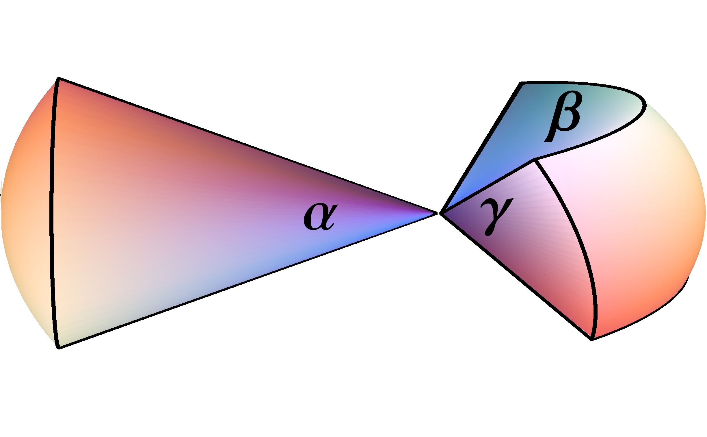
Figure 2: The two survey geometries considered (separately). A simple cone with one single opening angle $\alpha$ and a slice given by two angles $\beta$ and $\gamma$.

Equations (47) to (51) are interesting in two respects: Firstly, our expression for $\delta H_{{\cal D}}$ is simpler than the one in Umeh et al. (2010), nevertheless, both results agree. Secondly, Eqs. (47) to (51) quantify the connection between fluctuations in cosmological parameters and inhomogeneities in the distribution of matter. If we choose ”today” as our reference value, Eqs. (47) to (50) allow us to predict the domain averaged cosmological parameters:

$$\begin{array}[]{ccllcl}H_{{\cal D}}&=&H_{0}&\pm&\frac{1}{3}H_{0}\,f_{{\cal D}_{0}}&\sigma_{{\cal D}_{0}}\\ \Omega_{m}^{{\cal D}}&=&\Omega_{m}&\pm&\Omega_{m}\left(1+\frac{2}{3}f_{{\cal D}_{0}}\right)&\sigma_{{\cal D}_{0}}\\ \Omega_{{\cal R}}^{{\cal D}}&=&0&\pm&\left(\Omega_{m}+\frac{2}{3}f_{{\cal D}_{0}}\right)&\sigma_{{\cal D}_{0}}\\ \Omega_{\Lambda}^{{\cal D}}&=&\Omega_{\Lambda}&\pm&\frac{2}{3}\Omega_{\Lambda}\,f_{{\cal D}_{0}}&\sigma_{{\cal D}_{0}}\end{array}$$ (52)

with

$$f_{{\cal D}_{0}}\equiv f_{\cal D}\left(a_{{\cal D}_{0}}\right)=\frac{\Omega_{m}}{2}\left(5D_{0}^{-1}-3\right)\approx\left\{\begin{array}[]{ll}0.5&\Lambda\mathrm{CDM}\\ 1.0&\mathrm{EdS}\end{array}\right.,$$ (53)

where we assumed $\Omega_{m}=0.3$ for $\Lambda\mathrm{CDM}$. More generally, for $\Omega_{m}>0.1$, $f_{{\cal D}_{0}}$ may be approximated by (Lahav et al., 1991; Eisenstein & Hu, 1998)

$$f_{{\cal D}_{0}}\approx\frac{1}{140}\left(2+140\,\Omega_{m}^{4/7}-\Omega_{m}-\Omega_{m}^{2}\right).$$ (54)

From the knowledge of $\sigma_{{\cal D}_{0}}$ we may therefore easily derive the variation of cosmological parameters. To relate our calculations to real surveys, we elaborate in the next section on how to calculate $\sigma_{{\cal D}_{0}}$ for several survey geometries.

5 The effect of the survey geometry

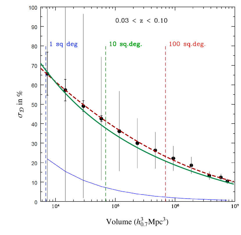
Figure 3: Variance of the matter density, $\sigma_{\cal D}$, as a function of the observed domain volume. Data were derived from the SDSS main sample by Driver & Robotham (2010). The dashed (red) line shows the fit of Driver & Robotham (2010) to the data, the solid (green) line is our result including the sample variance [solid (blue) line at the bottom].

Observations of the universe are rarely full–sky measurements and typically sample domains much smaller than the Hubble volume. We therefore must address the problem of the survey geometry. Effects from a limited survey size are in particular important for deep fields, as studied for example in Moster et al. (2010). While in their case, for small angles and deep surveys, approximating the observed volume by a rectangular geometry is appropriate, it probably is not appropriate for the bigger survey volumes that we have in mind.

We therefore chose two different geometries that resemble observationally relevant ones. Firstly, we used a simple cone with a single opening angle $\alpha$. The second geometry is a slice described by two angles $\beta$ and $\gamma$ for the size in right ascension and declination respectively. In the radial direction we assumed a top hat window, whose cut–off value corresponds to the depth of the survey. Both shapes are shown in Fig. 2.

To calculate $\sigma_{{\cal D}_{0}}$ for both geometries, we used a decomposition into spherical harmonics. This allowed us to derive an expression for the expansion coefficients in terms of a series in $\cos\left(2n\alpha\right)$ for the cone and a similar one for the slice, depending on trigonometric functions of $\beta$ and $\gamma$. The radial coefficients were calculated numerically using the $\Lambda$CDM power spectrum of Eisenstein & Hu (1998), including the effect of baryons on the overall shape and amplitude of the matter power spectrum, but without baryon acoustic oscillations.

All plots use best-fit $\Lambda$CDM values as given in Komatsu et al. (2011); $\Omega_{b}=0.0456$, $\Omega_{cdm}=0.227$ and $n_{s}=0.963$. The power spectrum is normalized to $\sigma_{8}=0.809$.

To ensure that the result of our calculation for the slice-like geometry and a standard $\Lambda$CDM power spectrum is reasonable, we compared it with an analysis of SDSS data by Driver & Robotham (2010). In Fig. 3 we show this comparison of their r.m.s. matter overdensity $\sigma_{\cal D}$ obtained from the SDSS main galaxy sample, in terms of its angular extension (and hence the volume). The dashed line going through the points shows their empirical fit to the data. The solid green line shows our result for the cosmic variance of a slice with respective angular extension (for $\beta=\gamma$), plus their sample variance. Note that our result is not a fit to SDSS data, but is a prediction based on the WMAP 7yr data analysis. Additionally, the real SDSS window function is slightly more complicated than our simplistic window, thus perfect agreement is not to be expected.

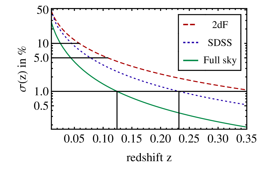
Figure 4: Variance of the matter density, $\sigma_{\cal D}$, for survey geometries resembling the 2dFGRS, the SDSS and a hypothetical full sky survey as a function of maximum redshift considered. We find that the determination of the local $\sigma_{\cal D}$ below redshifts of $0.1$ (corresponding to $\sim 400$ Mpc) is fundamentally limited by cosmic variance to the $1\%$ level.

For the full SDSS volume, $\sigma_{{\cal D}_{0}}$ is shown in Fig. 4. For comparison we also added the smaller, southern hemisphere 2dF survey and a hypothetical full sky survey. For the two surveys, we assumed an approximate angular extension of 120°$\times$60° for SDSS and for the two fields of the 2dF survey 80°$\times$15° and 75°$\times$10°. The ongoing BOSS survey corresponds to the plot for the SDSS geometry because it will basically have the same angular extension. Because it will target higher redshifts, it is not in the range of our calculation, however. As a rough statement (the precise value depends on the redshift), one may say that the 2dF survey is a factor of 5 and the SDSS survey a factor of 2.5 above the variance of a full sky survey. This is interesting because the SDSS survey covers approximately only $1/6$ of the full sky and the 2dF survey only $1/20$. This is due to the angular dependence of $\sigma_{\cal D}$. We find that fluctuations drop quickly as we increase small angles and flattens at large angles.

From Fig. (4) we see that the cosmic variance of the matter density for the SDSS geometry is 5% at a depth of $z\approx 0.08$ and still 1% out to $z\approx 0.23$. Note, however, that the extension of the domain of (spatial) averaging to a redshift of $0.35$ is clearly not very realistic because lightcone effects will become relevant with increasing extension of the domain. The assumption that this domain would be representative for a part of the hypersurface of constant cosmic time becomes questionable. We expect, however, that in this range evolution effects will only be a minor correction to the result presented here because of the following estimation:

The main effect we miss by approximating the lightcone by a fixed spatial hypersurface is evolution in the matter density distribution. To specify what ”region that is not too extended spatially” means, one should therefore estimate the maximum evolution in a given sample. This can be done by determining the growth of the density contrast in the outermost (and therefore oldest) regions of the sample. In the linear regime considered here, the evolution of the density contrast is given by $\delta\left(z\right)=\delta_{0}D\left(0\right)/D\left(z\right)$. Therefore, lightcone corrections should be smaller than $\epsilon_{l}=1-D\left(z\right)/D\left(0\right)$ which is $\epsilon_{l}\approx 5\%$ for $z=0.1$ and $\epsilon_{l}\approx 14\%$ for $z=0.3$. Therefore, the order of magnitude of our results should be correct on a wider range of scales, but on scales above $z=0.3$ the corrections to our calculation are expected to pass beyond $15\%$.

Finally, it should be noted that for large volumes the actual shape of the survey geometry is not very important. As long as all dimensions are bigger than the scale of the turnover of the power spectrum, the deviation of the cosmic variance for our shapes, compared to those of a box of equal volume, is at the percent level. To reach this result, we compared $\sigma_{{\cal D}_{0}}$ for the slice–like geometry to its value for a rectangular box of the same volume. We used a slice for which $\beta=\gamma$. The box was constructed to have a quadratic basis and the same depth as the slice in radial direction. Therefore the base square of the box is smaller than the square given by the two angles of the slice. The result of this comparison is that the deviation of $\sigma_{{\cal D}_{0}}^{rect}$ from the value for the slice is at most 6% for angles above $\beta\approx 10\text{\textdegree}$. For smaller angles the deviation becomes bigger and redshift–dependent. This is caused by the changing shape of the power spectrum at small scales. The large angle behavior confirms an observation of Driver & Robotham (2010). They found that the cosmic variance in the SDSS dataset was the same for both of the two geometries they considered.

6 Fluctuations of the curvature parameter

After the general study of the effect of the shape of the observational domain ${\cal D}$ on $\sigma_{{\cal D}_{0}}$, one may ask for which parameter the fluctuations are most important.

The three lowest lines in the plot of Fig. 5 show that this is the case for the curvature fluctuations. The two lowest lines, showing the fluctuations $\delta\Omega_{m}$ and $\delta H_{{\cal D}_{0}}/H_{{\cal D}_{0}}$ for the full sphere, lie a factor of 1.6 and 3.8, respectively, below the respective curvature fluctuations $\delta\Omega_{{\cal R}}^{{\cal D}}$. Therefore the fluctuations of $\Omega_{m}$ play a smaller role for all universes with $\Omega_{m}<1$. The uncertainty in $H_{{\cal D}_{0}}$, which has been in the focus of the investigations so far (Shi et al., 1996; Li & Schwarz, 2008; Umeh et al., 2010), contributes even less to the distortion of the geometry, as we shall discuss in Section 7.

What this means for real surveys, such as the 2dF or the SDSS survey, is shown by the three upper lines in Fig. 5. They compare $\delta\Omega_{{\cal R}}^{{\cal D}}$ for the slices observed by these surveys to that of a full sky measurement. $\delta\Omega_{{\cal R}}^{{\cal D}}$ is bigger than one percent up to a redshift of $0.18$ for the SDSS and $0.28$ for the 2dF survey and it does not drop below $0.001$ for values of $z$ as high as $0.5$. This may seem very low, but it has been shown that getting the curvature of the universe wrong by $1\permil$ already affects our ability to measure the dark energy equation of state $w\left(z\right)$ (Clarkson et al., 2007). Of course one has to keep in mind that for high redshifts one has to be careful with the values presented here because they are based on the assumption that the observed region lies on one single spatial hypersurface. Because this approximation worsenes beyond a redshift of $0.1$, there may be additional corrections to the size of the fluctuations stemming from lightcone effects.

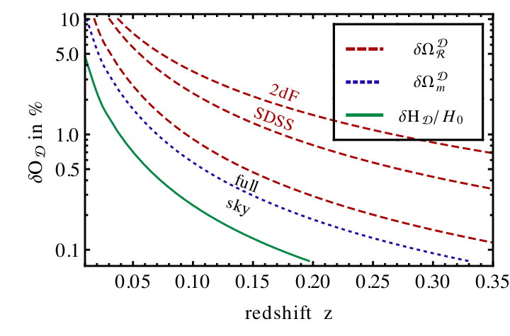
Figure 5: Top three lines: the expected r.m.s. fluctuation of the curvature parameter, $\delta\Omega_{{\cal R}}^{{\cal D}}$, for geometries resembling the 2dFGRS, the SDSS, and a full sky. The two lowest lines are the expected r.m.s. fluctuations of the parameters $\Omega_{m}^{{\cal D}_{0}}$ and $H_{{\cal D}_{0}}$ for a full–sky survey extending to the respective redshift. The curvature fluctuations turn out to be higher than all other fluctuations.

To investigate the curvature fluctuations for more general geometries, we show in Fig. 6 the angular and radial dependence of the curvature fluctuation $\delta\Omega_{{\cal R}}^{{\cal D}}\left(\alpha\right)$ for the cone-like window of Fig. 2.

On the l.h.s. of Fig. 6 we evaluate the angular dependence. For a survey that only reaches a redshift of $0.1$, the fluctuations are still higher than $0.01$ for a half–sky survey. It is interesting to note that for a deeper survey, $\delta\Omega_{{\cal R}}^{{\cal D}}\left(\alpha\right)$ grows much faster when $\alpha$ is reduced than for a shallow survey. This is because $\sigma_{{\cal D}_{0}}\left(R\right)$ changes from a relatively weak $R^{-1}$ decay to a $R^{-2}$ decay on larger scales. For $z=0.35$, this behavior dominates and a decrease in $\alpha$ increases $\sigma_{{\cal D}_{0}}\left(R,\alpha\right)$ stronger than in the $R^{-1}$ regime.

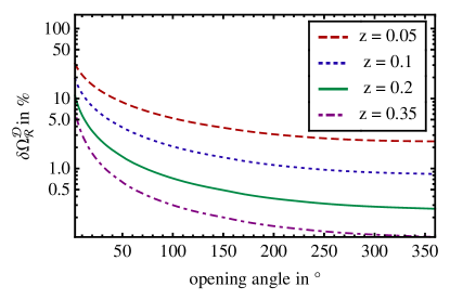
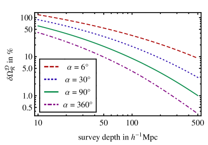
Figure 6: Cosmic variance of the curvature parameter. Left panel: Dependence of $\delta\Omega_{{\cal R}}^{{\cal D}}$ on the opening angle of the cone-like survey geometry of Fig. 2 for different top hat depths of the survey. Right panel: Dependence of $\delta\Omega_{{\cal R}}^{{\cal D}}$ on the depth of the survey. For a small cone of 6° opening angle we expect curvature fluctuations of 10% up to $450h^{-1}\mathrm{Mpc}$.

On the r.h.s. of Fig. 6 we show the dependence of $\delta\Omega_{{\cal R}}^{{\cal D}}$ on the survey depth for some opening angles of the cone-like window. For narrow windows the fluctuation in $\Omega_{{\cal R}}^{{\cal D}}$ stays high, even beyond the expected homogeneity scale of $100h^{-1}\mathrm{Mpc}$. For $R=200h^{-1}\mathrm{Mpc}$ and a $6\text{\textdegree}$ window, for example, it is still at $\delta\Omega_{{\cal R}}^{{\cal D}}\approx 0.2$. For smaller beams these fluctuations persist even out to much longer distances. Therefore they play an important role for deep field galaxy surveys, as shown in Moster et al. (2010); Driver & Robotham (2010) for the matter density fluctuations. But even for wider angles, fluctuations in curvature persist on sizeable domains. If one recalls that the distance given for the full sphere of 360° is its radius, this means that regions in the Universe as big as $540h^{-1}\mathrm{Mpc}$ have typical curvature fluctuations on the order of 1%. This is not that small because the last scattering surface at $z\approx 1100$ is only $9600h^{-1}\mathrm{Mpc}$ away. One of these regions therefore fills more than 5% of the way to that surface.

To put these values into perspective, we compare the WMAP 5yr confidence contours (Komatsu et al., 2009) on the curvature parameter with those that may in principle be derived from the 2dF or the SDSS survey in Fig. 7. Because they only sample a finite size of the Universe, one cannot be sure that this value is indeed the background value and not only a local fluctuation. The cosmic variance induced by this finite size effect is, for the 2dF survey volume up to $z\approx 0.2$, shown by the two second–largest (red) ellipses. The two innermost (blue) ones depict the minimum possible error using the SDSS survey volume up to $z\approx 0.3$. Clearly, the determination of $\Omega_{{\cal R}}^{{\cal D}}$ may perhaps be improved by a factor of two if one were to eliminate all other sources of uncertainty. This may be less if lightcone effects play a non–negligible role already for $z\approx 0.3$.

Fig. 8 shows the dependence of the curvature fluctuation on the considered cosmology. For this study we fixed the spectral index and the normalization of the spectrum to $n_{s}=0.963$ and $\sigma_{8}=0.809$, respectively. We varied each of the other parameters one after another, while keeping the remaining ones fixed to the concordance values. We used the SDSS geometry out to a redshift of $z=0.09$ as a reference value at which we conducted this investigation, because the concordance values lead to a $\delta\Omega_{{\cal R}}^{{\cal D}}$ of $0.01$ for this configuration. Interestingly enough, the dependence on the $\Omega_{m}$ parameter is very weak. This means that the value does not differ much for the flat $\Lambda$CDM model and the EdS model. This is surprising, because the prefactor of $\sigma_{{\cal D}_{0}}$ in (49) changes by a factor of 3 from about 5/11 for $\Lambda$CDM to 5/3 for EdS. This rise, however, is compensated for by a drop of the value of $\sigma_{{\cal D}_{0}}$. The reason for this drop is that a higher $\Omega_{m}$ leads to more power on small scales. Because we kept the integrated normalization fixed at a given value of $\sigma_{8}$, this means less power on large scales, i.e. at $z=0.09$. Moreover, a variation of the Hubble constant $h$ and the baryon fraction $f_{b}$ has only a small effect around the concordance value. $\delta\Omega_{{\cal R}}^{{\cal D}}$ changes significantly only for more extreme values of $f_{b}$ and $h$.

7 Fluctuations of the acoustic scale

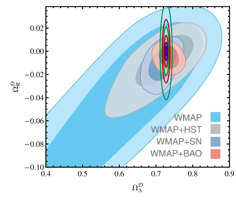
Figure 7: Minimum confidence contours in $\Omega_{\Lambda}^{\cal D}$ and $\Omega_{{\cal R}}^{{\cal D}}$ achievable in different volumes through fluctuations of matter. The green (outermost) ellipses are the $95\%$ and $68\%$ contours for the volume from which the HST data are drawn. The next inner (red) ones are for a survey of the size of the 2dF survey up to $z=0.2$. In the middle there is a small double ellipse in blue, showing the values for the SDSS volume up to $z=0.3$. The background image depicts the results from WMAP 5 (Komatsu et al., 2009). They give the experimental values and uncertainties on these parameters for a combination of various experimental probes.

Let us now turn to the effect of fluctuations caused by inhomogeneities on the local distance estimates. An important distance measure, recently used in BAO experiments, is $D_{V}$. It was introduced in Eisenstein et al. (2005) and mixes the angular diameter distance and the comoving coordinate distance to the BAO ring. It is measured through the BAO radius perpendicular to the line of sight $r_{\perp}$ and the comoving radius parallel to the line of sight $r_{\parallel}$.

$$r_{bao}:=\left(r_{\parallel}r_{\perp}^{2}\right)^{\frac{1}{3}}=D_{V}\left(z\right)\Delta\theta^{2}\frac{\Delta z}{z}$$ (55)

One can, therefore, determine the distance $D_{V}$ to the corresponding redshift, if the comoving radius of the baryon ring $r_{bao}$ is known. This may be achieved by a measurement of the angle of the BAO ring on the sky $\Delta\theta$ and its longitudinal extension $\Delta z/z$. The precise definition of $D_{V}$ is derived from the expressions of the comoving distances $r_{\parallel}$ and $r_{\perp}$:

$$r_{\parallel} = \intop_{z}^{z+\Delta z}\frac{c}{H(z^{\prime})}{\rm d}z^{\prime}\approx\frac{c\Delta z}{H(z)}=\frac{cz}{H(z)}\frac{\Delta z}{z},$$ (56)

$$r_{\perp} = \left(1+z\right)D_{A}(z)\Delta\theta,$$ (57)

from which we find

$$D_{V}(z)=\left(\frac{cz}{H(z)}D_{M}^{2}(z)\right)^{\frac{1}{3}},$$ (58)

where $D_{M}$ is the comoving angular distance

$$D_{M}(z)=c\left(\sqrt{\Omega_{k}}H_{0}\right)^{-1}\sinh\left(\sqrt{\Omega_{k}}I\left(z\right)\right),$$ (59)

with

$$I(z)=\intop_{0}^{z}\frac{H_{0}}{H(z^{\prime})}{\rm d}z^{\prime}.$$ (60)

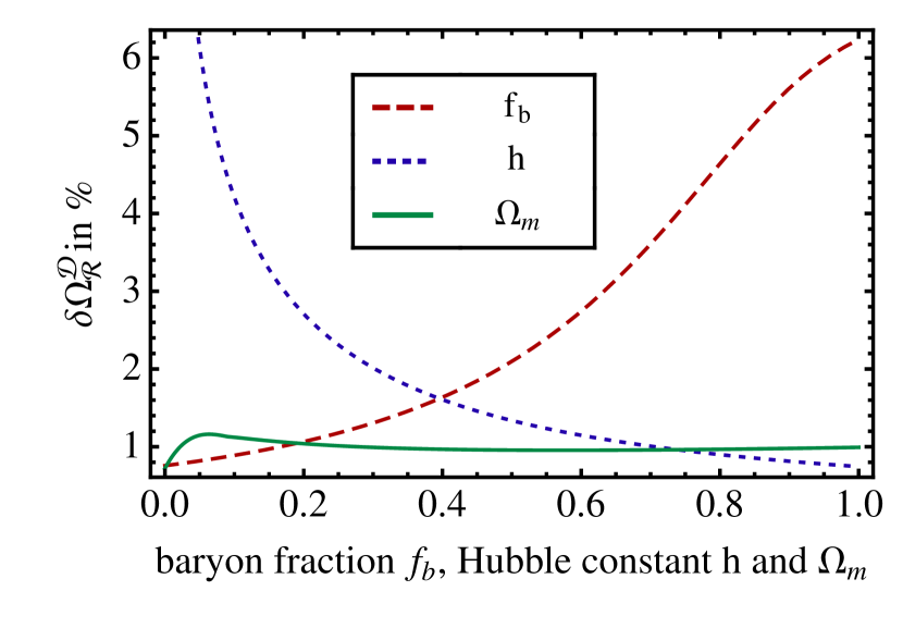
Figure 8: Dependence of $\delta\Omega_{{\cal R}}^{{\cal D}}$ on some cosmological parameters for a spherical domain extending to $z=0.09$. The basis is the $\Lambda$CDM model with $\Omega_{b}=0.0456$, $\Omega_{cdm}=0.227$, $h=0.7$, $n_{s}=0.963$ and $\sigma_{8}=0.809$. For this model and for the chosen redshift, $\delta\Omega_{{\cal R}}^{{\cal D}}\approx 0.01$. We then varied $\Omega_{m}=\Omega_{b}+\Omega_{cdm}$, $f_{b}=\Omega_{b}/\Omega_{m}$ and $h$ between $0$ and $1$, holding the other parameters fixed at their aforementioned values. Because $\sigma_{8}$ is fixed, the fluctuation in $\Omega_{{\cal R}}^{{\cal D}}$ is nearly independent on $\Omega_{m}$.

As already mentioned above, the term $\Omega_{{\cal Q}}^{{\cal D}}$ vanishes in our first–order treatment and the curvature contribution scales as $a_{{\cal D}}^{-2}$. Therefore we may express the Hubble rate as

$$\frac{H_{{\cal D}}(z)}{H_{{\cal D}_{0}}}=\left[(1+z)^{3}\Omega_{m}^{{\cal D}_{0}}+(1+z)^{2}\Omega_{{\cal R}}^{{\cal D}_{0}}+(1-\Omega_{m}^{{\cal D}_{0}}-\Omega_{{\cal R}}^{{\cal D}_{0}})\right]^{\frac{1}{2}},$$ (61)

where we assumed the relation between redshift and average scale factor of Eq. (25). We may now calculate the fluctuation of $D_{V}$,

$$\frac{\delta r_{\parallel}}{r_{\parallel}} = \frac{\delta H_{{\cal D}_{0}}}{H_{{\cal D}_{0}}}+\left|\frac{1-(1+z)^{2}}{2}\frac{H_{{\cal D}_{0}}^{2}}{H_{{\cal D}}(z)^{2}}\right|\delta\Omega_{{\cal R}}^{{\cal D}_{0}}$$ (62)

$$+\left|\frac{1-(1+z)^{3}}{2}\frac{H_{{\cal D}_{0}}^{2}}{H_{{\cal D}}(z)^{2}}\right|\delta\Omega_{m}^{{\cal D}_{0}}$$

$$\frac{\delta r_{\perp}}{r_{\perp}} = \frac{\delta D_{M}}{D_{M_{0}}}=\frac{\delta H_{{\cal D}_{0}}}{H_{{\cal D}_{0}}}+\left|\frac{I(z)^{2}}{6}+\frac{I^{\prime}(z)}{I(z)}\right|\delta\Omega_{{\cal R}}^{{\cal D}_{0}}$$ (63)

$$+\left|\frac{I^{\prime}(z)}{I(z)}\right|\delta\Omega_{m}^{{\cal D}_{0}}$$

$$\frac{\delta D_{V}}{D_{V}} = \frac{1}{3}\frac{\delta r_{\parallel}}{r_{\parallel}}+\frac{2}{3}\frac{\delta r_{\perp}}{r_{\perp}}$$ (64)

where $I^{\prime}(z)$ denotes a partial derivation with respect to the respective parameter, i.e. $\Omega_{{\cal R}}^{{\cal D}_{0}}$ or $\Omega_{m}^{{\cal D}_{0}}$. Note that $I^{\prime}(z)$ and $I(z)$ are evaluated on the background ($\Omega_{{\cal R}}^{{\cal D}_{0}}=0$ and $\Omega_{m}^{{\cal D}_{0}}=\Omega_{m}$).

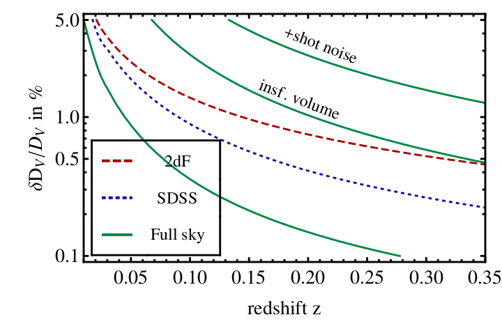
Figure 9: Errors on the distance $D_{V}$ for various survey geometries as a function of maximum redshift. For comparison the error induced by the finite number of BAO modes in the corresponding full sphere volume, calculated with the fitting formula of Seo & Eisenstein (2007), is shown (insufficient volume). This error is about a factor of $10$ bigger than the error from the local volume distortion caused by inhomogeneities that we calculated. Adding a shot noise term, corresponding to a galaxy density of $n=3\times 10^{-4}h^{3}\mathrm{Mpc^{-3}}$ typical for SDSS and BOSS, we find that the cosmic variance of $D_{V}$ is a subdominant contribution to the error budget.

We evaluated the magnitude of the fluctuations in $D_{V}$, based on the cosmological parameters of the concordance model, as presented in Fig. 9. Fluctuations as low as one per cent are reached for much smaller domains than for the cosmic variance of the $\Omega$-parameters. Thus, at first sight it might seem that the BAO measurement of $D_{V}$ could essentially overcome the cosmic variance limit. Closer inspection of this result reveals that this is not the case. Indeed, the much smaller variation of the distance $D_{V}$ means that a precise knowledge of the distance measure $D_{V}$ does not lead to an equivalently good estimate of the cosmic parameters.

Clearly, the systematic uncertainty that we calculated is only a minor effect compared with the errors intrinsic to the actual measurement of the acoustic scale, as a comparison of the three solid (green) lines in Fig. 9 shows. The lowest one is the fluctuation of the scale $D_{V}$ for full spheres of the corresponding size at different places in the universe. It is therefore the possible local deformation caused by statistical over- or underdensities. The possible precision of a measurement of $D_{V}$ by BAOs, however, also depends on the number of observable modes. This induces an error if the volume is too small, and in particular when it is smaller than the BAO scale a reasonable measurement is no longer possible. Accordingly, even for a perfect sampling of the observed volume, the error will not be smaller than the solid (green) lines in the middle. If one adds shot noise caused by imperfect sampling by a galaxy density of $n=3\times 10^{-4}h^{3}\mathrm{Mpc^{-3}}$, typical for SDSS and BOSS, the error increases even more. This means that for the realistic situation where we do not have a sufficiently small perfect ruler to allow for large statistics already for the small volumes considered here, the deformation uncertainty that we calculated remains completely subdominant.

8 Fluctuations of the Hubble scale

Local fluctuations of the Hubble expansion rate have already been considered in the literature (Turner et al., 1992; Shi et al., 1996; Wang et al., 1998; Umeh et al., 2010). Here we wish to add two new aspects.

The first one is on the measurement of $H(z)$ itself. Experiments that try to measure $H$ as a function of $z$, like the WiggleZ survey (Blake et al., 2011), do this by measuring a “local” average $H(z_{m})$ in a region around the redshift $z_{m}$. These regions should not be too small to keep the effects of local fluctuations small. On the other hand they cannot be enlarged in an arbitrary way because then the redshift $z_{m}$ becomes less and less characteristic for the averaging domain. In other words, for an increasingly thicker shell $\Delta z$, the evolution of $H(z)$ begins to play a role. Therefore, one may find the optimal thickness of the averaging shells over which the variation in the expansion rate

$${\rm Var}\left[H(z)\right] = \frac{1}{V_{{\cal D}}}\intop H[z(r)]^{2}W_{{\cal D}}\left(r\right){\rm d}^{3}r$$ (65)

$$-\left(\frac{1}{V_{{\cal D}}}\intop H[(z(r)]W_{{\cal D}}\left(r\right){\rm d}^{3}r\right)^{2}$$

equals the variance imposed by the inhomogeneous matter distribution. The corresponding shells are shown in Fig. 10. It should be noted that the error for the first bin is certainly underestimated in our treatment, which rests on linear perturbation theory. Taking into account higher orders, which become dominant at small scales, will certainly increase it. Of course, in these measurements the survey geometries will not necessarily be close to the SDSS or the 2dF geometry, but they are shown to illustrate survey geometries that do not cover the full sky.

Figure 10: Optimum thickness of shells to minimize the variance of $H\left(z\right)$ (see text for the two competing effects). The respective error corresponds to the height of the bars, the shells necessary for this purpose to their width.

Secondly, we wish to note that the relation between fluctuations in the Hubble expansion rate and fluctuations in the matter density offers the interesting possibility to determine the evolution of the growth function for matter perturbations from the variances of the Hubble rate measured at different redshifts. A direct measurement of the growth function by a determination of $\sigma_{8}$ at different epochs is difficult, because one never examines the underlying dark matter distribution. Therefore one has to assume that the observed objects represent the same clustering pattern as the underlying dark matter (this is the problem of bias). It is well known that there is bias and its modeling typically has to rely on assumptions.

An interesting bypass is to look at the variation of local expansion rates at different redshifts. The assumption that the luminous objects follow the local flow is more likely and the assumption that this local flow is generated by the inhomogeneities of the underlying dark matter distribution is also reasonable. A similar idea leads to the attempt to use redshift-space distortions to do so (Percival & White, 2009). The fact that one considers fluctuations means that we would not have to know the actual value of $H\left(z\right)$, but only the local variation at different redshifts.

This variation, defined as

$$\delta_{H}=\frac{H_{{\cal D}}-\overline{H}_{{\cal D}}(a_{{\cal D}})}{\overline{H}_{{\cal D}}(a_{{\cal D}})}\;,$$ (66)

has the fluctuations of Eq. (47)

$$\sigma\left(\delta_{H}\right)=\frac{1}{3}\overline{H_{{\cal D}}}\left(a_{{\cal D}}\right)f_{\cal D}\left(a_{{\cal D}}\right)\sigma_{{\cal D}_{0}}\;.$$ (67)

If we were to measure this quantity at different redshifts, we could, without knowledge of the absolute normalization of $H_{{\cal D}}\left(z\right)$, determine $f_{\cal D}\left(a_{{\cal D}}\right)$ only from the variance and therefore the constant $c=\Omega_{\Lambda}/\Omega_{m}$.

Note that in the standard case, where the background redshift is identified with the observed one, $f_{\cal D}\left(a_{{\cal D}}\right)$ is simply replaced by the growth rate $f\left(a\right)=\frac{{\rm d}\ln D\left(a\right)}{{\rm d}\ln a}$, and measuring the Hubble fluctuations would yield a direct measurement of $f$. In the real world, where the redshift captures the structure on the way from the source to us, it is not directly the background redshift. One would rather measure the modified ”growth rate” $f_{\cal D}\left(a_{{\cal D}}\right)$. The difference between these two quantities is small in our range of validity for $f_{\cal D}\left(a_{{\cal D}}\right)$, however (corrections of linear order in the perturbations).

9 Conclusion

For the first time, we brought together the well–established perturbative approach to incorporate inhomogeneities in Friedman-Lemaître models (the theory of cosmological perturbations) and the ideas of cosmological backreaction and cosmic averaging in the Buchert formalism. Focusing on observations of the large–scale structure of the Universe at late times, we showed that the cosmic variance of cosmological parameters is in fact the leading order contribution of cosmological averaging.

We studied volume averages, their expected means, and variances of the cosmological parameters $H_{0},\Omega_{\cal R},\Omega_{m},\Omega_{\Lambda}$ ($\Omega_{\cal Q}$ is of higher order in perturbation theory). Our central result is summarized in (47)–(51).

Our extension of the backreaction study of Li & Schwarz (2008) to the $\Lambda$CDM case enabled us to study fluctuations for a wider class of cosmological models. We were able to confirm for the fluctuations in the Hubble rate that our results in comoving synchronous gauge agree with those found in Poisson gauge (Umeh et al., 2010).

The use of general window functions allowed us to consider realistic survey geometries in detail and to calculate the fluctuations in the matter density, empirically found in the SDSS data by Driver & Robotham (2010), directly from the underlying DM power spectrum. Converting this information into curvature fluctuations, we found that regions of $540h^{-1}\mathrm{Mpc}$ diameter may still have a curvature parameter of $\sim 0.01$, even if the background curvature vanishes exactly. We found that cosmic variance is a limiting factor even for surveys of the size of the SDSS survey. A volume–limited sample up to a redshift of $0.5$ was able to constrain the local curvature to $0.1$ per cent.

Finally, we investigated the distortions of the local distance to a given redshift and found that it is less affected by the fluctuations of the local cosmic parameters than one might expect. The distance measure $D_{V}$, used in BAO studies, is accurate to $0.2$ percent for samples ranging up to $z\approx 0.35$. This means that BAO studies are not limited by cosmic variance, but by problems such as sampling variance and insufficient volume, as discussed in section 7.

In a next step one should incorporate the second–order effects into the expected means of the cosmological parameters. There are no second–order corrections to the variances, as argued in section 2. Therefore a complete second–order treatment seems feasible.

The limitation of our approach comes from the fact that Buchert’s formalism relies on spatial averaging. Averaging on the light cone would be more appropriate (Gasperini et al., 2011), thus the study in this work has been restricted to redshifts $\ll 1$, where we expect light cone effects to play a subdominant role.