Probing the quantum state of a 1D Bose gas using off-resonant light scattering

Abstract

We present a theoretical treatment of coherent light scattering from an interacting 1D Bose gas at finite temperatures. We show how this can provide a nondestructive measurement of the atomic system states. The equilibrium states are determined by the temperature and interaction strength, and are characterized by the spatial density-density correlation function. We show how this correlation function is encoded in the angular distribution of the fluctuations of the scattered light intensity, thus providing a sensitive, quantitative probe of the density-density correlation function and therefore the quantum state of the gas.

The remarkable progress made in cold atom physics over the past two decades has been facilitated by the precision and flexibility of the measurement tools available to experimentalists. Optical probing by lasers has proved to be one of the most important tools, for example absorption and phase contrast imaging Ketterle_probe have been extensively used to measure atomic density in bosonic and fermionic systems. Proposals for employing coherent light scattering from cold atoms are long standing javanainen_ruo . More than a decade ago superradiant light scattering from a Bose condensate was demonstrated, and stimulated light scattering was used to implement Bragg scattering of matter waves Ketterle_super_and_bragg . More recently Mekhov et al ritsch have proposed light scattering as a probe of cold atoms in an optical lattice.

In this letter we present a theoretical treatment of monochromatic light scattering appropriate for a 1D Bose gas. We show that for far detuned incident light, a clear signature of various quantum states of the gas can be obtained from the fluctuations of the scattered light. The 1D Bose gas is an important model in many-body physics, providing one of the simplest paradigms of a strongly interacting system, owing to its exact integrability via the Bethe ansatz liebliniger . In addition, the distinction between fermions and bosons (that are well known in 3D systems), are suppressed in 1D cheon_shigehara . For a 1D Bose gas with repulsive interactions, the system state can be characterized by the two body spatial density-density correlation function correlations1 . Possible system states range from a nearly ideal gas in the ‘high’ temperature regime (where the spatial correlation function displays bunching), to the Tonks-Girardeau gas in the interaction dominated regime, (where the correlation function displays antibunching). Experimental investigations of the 1D Bose gas have been pursued in recent years bec_low_dim_expts . A method for measuring momentum correlations of a cold atom system has been demonstrated by analysing the density fluctuations of a resonant absorption image Altman2004_GreinerJin2005 . Two and three body correlations were also studied via resonant absorption images karen_expts . Impressive as these experiments are, this technique cannot image submicron density fluctuations. In this work we show that a nondestructive measurement of the spatial nonlocal density-density correlation function of a 1D Bose gas can be made by measuring the angular distribution of the fluctuations in the scattered light intensity.

We consider a system of two-state bosonic atoms in a long thin cylindrical trap, illuminated by a coherent laser beam of frequency $\omega_{\rm L}$ and wavevector ${\bf k}_{\rm L}$. Each atom has resonant frequency $\omega_{0}$ and transition dipole moment ${\mathbf{d}}$. We use the rotating wave approximation for the radiation interaction. The laser mode is treated as a classical quantity ${\mathbf{E}_{\rm L}}e^{i\left({\bf k_{\rm L}}\cdot\mathbf{x}-\omega_{\rm L}\right)t}$, and its interaction with the atoms is characterised by the detuning $\Delta_{{\rm L}}=\omega_{{\rm L}}-\omega_{0}$ and the Rabi frequency $\Omega_{{\rm L}}={\mathbf{d}}\cdot{\mathbf{E}_{\rm L}}/\hbar$. In the case where the detuning is large, $\Delta_{{\rm L}}\gg\Omega_{\rm L},\Gamma$, ($\Gamma$ is the spontaneous emission rate) the upper internal atomic state can be adiabatically eliminated, leaving coupled equations for the scattered radiation modes $\hat{a}_{\mathbf{k}}(t)$ and the atomic field operator for the lower internal state $\hat{\Psi}({\bf x})$. The equation for $\hat{a}_{\mathbf{k}}(t)$ can be integrated, (ignoring small terms and employing the Markov approximation) leading to

$$\hat{a}_{\mathbf{k}}(t)=\frac{\pi\Omega_{\rm L}g_{\mathbf{k}}}{\Delta_{\rm L}}e^{-i\omega_{\rm L}t}\delta(\Delta_{\mathbf{k}})e^{i\Delta_{\bf k}t/2}\int_{\mathbb{S}^{3}}\!d^{3}\!\mathbf{x}\;e^{i{\bf q}\cdot{\bf x}}\hat{\rho}({\bf x},t).$$ (1)

Here $g_{\mathbf{k}}$ denotes the usual atom-radiation coupling constant, $\Delta_{\mathbf{k}}=\omega_{\rm L}-\omega_{\mathbf{k}}$, $\hat{\rho}=\hat{\Psi}^{\dagger}\hat{\Psi}$ is the 3D density of the system, ${\bf q}={\bf k}_{\rm L}-{\bf k}$ and $\mathbb{S}^{3}$ is the region of space where the incoming light intersects the gas. We have excluded the additive quantum noise term from Eq. (1) as we will only consider normally ordered averages of $\hat{a}_{\mathbf{k}}$.

For the cylindrically symmetric trapping potential $V(\mathbf{x})=m\omega_{\perp}^{2}(y^{2}+z^{2})/2$, the 1D regime can be achieved when $\hbar\omega_{\perp}\ll k_{\rm B}T,\mu$ (the chemical potential). In addition the atomic recoil energy should be much less than $\hbar\omega_{\perp}$. In this case the atomic field operator is well approximated by $\hat{\Psi}(\mathbf{x},t)=(\sqrt{\pi}l_{\perp})^{-1}\exp[{-(y^{2}+z^{2})/2l_{\perp}^{2}}-i\omega_{\perp}t]\hat{\phi}(x,t)$, where $\hat{\phi}(x,t)$ is the 1D annihilation operator of the atomic ground state and $l_{\perp}=\sqrt{\hbar/(m\omega_{\perp})}$ is the transverse oscillator length. Performing the transverse integration in Eq. (1) gives

$$\hat{a}_{\mathbf{k}}(t)=A\;e^{-i\omega_{\rm L}t}\int_{\mathbb{S}^{1}}\!dx\;\hat{n}(x)e^{iq_{\rm x}x}$$ (2)

where $A={\pi\Omega_{\rm L}g_{\mathbf{k}}e^{i\Delta_{\bf k}t/2}\delta(\Delta_{\mathbf{k}})e^{-(q_{\rm y}^{2}+q_{\rm z}^{2})l_{\perp}^{2}/4}}/{\Delta_{\rm L}}$, $\hat{n}=\hat{\phi}^{\dagger}\hat{\phi}$ is the 1D density and $\mathbb{S}^{1}=[-L/2,L/2]$ is the region where the light intersects the gas. In this paper, we consider the case where the incident light is a plane wave polarized along the $z$ axis, with ${\bf k_{\rm L}}$ in the $x$-$y$ plane and making an angle $\theta_{\rm L}$ to the $y$ axis. The intensity of the scattered light is proportional to the total number of photons in a given mode,

$$\langle\hat{a}_{\mathbf{k}}^{\dagger}\hat{a}_{\mathbf{k}}^{\phantom{\dagger}}\rangle=\left|A\right|^{2}\left[N\!+\!2n^{2}\!\!\int_{0}^{L}dr\;g^{(2)}(r)\cos\left(q_{\rm x}r\right)\left(L-r\right)\right],$$ (3)

where $N=nL$ is the total number of atoms illuminated. The first term in the square brackets in Eq. (3) arises from the atomic shot noise, while the integral provides the effect of the atomic correlations, via the density-density correlation function of the gas, $g^{(2)}(x-x^{\prime})=\langle:\!\hat{n}(x)\;\hat{n}(x^{\prime})\!:\rangle/n^{2}$. We have assumed that, within the illuminated region, the density is constant, $\langle\hat{n}(x)\rangle=n$, and $g^{(2)}$ is translationally invariant.

The function $g^{(2)}$ characterises the state of a uniform density 1D Bose gas correlations1 . At equilibrium in the thermodynamic limit, $g^{(2)}(r)$ is completely determined by two parameterscorrelations2 : the dimensionless interaction strength $\gamma=m2\omega_{\perp}a/\hbar n$ (where $a$ is the 3D s-wave scattering length, and $m$ is the atomic mass) and the reduced temperature $\tau=T/T_{\rm d}$ where $T_{\rm d}=\hbar^{2}n^{2}/(2k_{\rm B}m)$ is the temperature of quantum degeneracy. Varying these two parameters gives rise to three physically distinct regimes, each of which can be further split into two subregimes.

(i) Nearly ideal-gas regime, $\gamma\ll\min\{\tau^{2},\sqrt{\tau}\}$. Here the temperature always dominates over the interaction strength, and the local density-density correlation displays thermal bunching, $1<g^{(2)}(0)\leq 2$. This regime has two subregimes defined by $\tau\ll 1$ (quantum decoherent gas) or $\tau\gg 1$ (classical decoherent gas).

(ii) Weakly interacting regime, $\tau^{2}\ll\gamma\ll 1$. This regime, for which both the interaction strength and the temperature are small, realises the quasicondensate where density fluctuations are strongly suppressed but long wavelength fluctuations of the phase still exist quasiconds . The density-density correlation is close to the uncorrelated value of $g^{(2)}(r)\approx 1$, and fluctuations occur due to either vacuum or thermal excitations. Two further subregimes can be defined, $\tau\ll\gamma$ (dominant vacuum fluctuations) or $\tau\gg\gamma$ (dominant thermal fluctuations).

(iii) Strongly interacting regime (Tonks gas), $\gamma\gg\max\{1,\sqrt{\tau}\}$. Here the interaction strength always dominates over temperature induced effects, and the local density-density correlation displays interaction-induced antibunching $0\leq g^{(2)}(0)<1$. This regime is usefully divided into two further subregimes defined by $\tau\ll 1$ (low temperature Tonks gas) and $\tau\gg 1$ (high temperature Tonks gas).

In each of the above regimes, perturbation theory can be applied and six different analytic expressions for the density-density correlation function have been calculated correlations2 . The density–density correlation function decays from its local value $g^{(2)}(0)$ to the uncorrelated value $g^{(2)}=1$ over a length $l_{c}$ ( the correlation length). For the quantum decoherent gas we have $l_{c}=2/(\tau n)$ (the phase coherence length), while for the classical decoherent gas, $l_{c}=\sqrt{4\pi/(\tau n^{2})}$ (the thermal de Broglie wavelength). For the weakly interacting quasicondensate regime, (with either vacuum or thermal fluctuations dominant) we have $l_{c}=1/\sqrt{\gamma n^{2}}$ (the healing length). For the low temperature Tonks gas we have $l_{c}=1/n$ and finally for the high temperature Tonks gas we have $l_{c}=\sqrt{4\pi/(\tau n^{2})}$

The physically relevant cases for light scattering are where $L\gg l_{c}>\lambda$. In order to distinguish the incoherent from the coherent scattering it is convenient to define $\eta(r)\equiv g^{(2)}(r)-1$, Eq. (3) then becomes

$$\langle\hat{a}_{\mathbf{k}}^{\dagger}\hat{a}_{\mathbf{k}}^{\phantom{\dagger}}\rangle = \langle\hat{a}_{\mathbf{k}}^{\dagger}\rangle\langle\hat{a}_{\mathbf{k}}^{\phantom{\dagger}}\rangle+\left|A\right|^{2}N\left[1+2\frac{N}{L^{2}}\int_{0}^{L}dr\;\eta(r)\cos\left(q_{\rm x}r\right)\left(L-r\right)\right].$$ (4)

The first term on the right of Eq. (4), $\langle\hat{a}_{\mathbf{k}}^{\dagger}\rangle\langle\hat{a}_{\mathbf{k}}^{\phantom{\dagger}}\rangle$, is the coherent scattering and is predominantly within angular width $\sim\lambda/L$ of the $q_{\rm x}=0$ direction. For $\lambda\ll L$, the total intensity of coherently scattered light at a distance $r$ from the gas is

$$I_{c}=N^{2}\left(\frac{\Omega_{\rm L}}{2\Delta_{\rm L}}\right)^{2}\Gamma\hbar\omega_{\rm L}\frac{3\sin^{2}\!\theta}{8\pi r^{2}}{\rm sinc}^{2}\!\left[\frac{L\Theta}{2}\right],$$ (5)

where $\Theta=k_{Lx}-k_{\rm L}\sin\theta\cos\theta_{s}$, and $\theta_{s}=\arctan(\frac{k_{x}}{k_{y}})$ is the in-plane scattering angle, and $\theta=\arctan(\frac{\sqrt{k_{x}^{2}+k_{y}^{2}}}{k_{z}})$ is the out-of-plane scattering angle (see Fig. 4).

The signature for the atomic $g^{(2)}(r)$ function is in the fluctuations of the scattered intensity arising from the integral term of Eq. (4). These fluctuations are typically expressed in terms of quadratures of the radiation field operator (relative to a particular phase reference $\beta$), which are defined by $\hat{X}_{\beta}^{{\mathbf{k}}}=\frac{1}{2}\left(\hat{a}_{\mathbf{k}}e^{-i\beta}+\textrm{h.c.}\right)$. The variances of these quadrature operators,

$$R_{\beta}^{\mathbf{k}} =\langle\left(\hat{X}_{\beta}^{{\mathbf{k}}}\right)^{2}\rangle-\langle\hat{X}_{\beta}^{{\mathbf{k}}}\rangle^{2}$$ (6)

$$=|A|^{2}N\left[\frac{1}{2}\!+\!\frac{N}{L^{2}}\int_{0}^{L}dr\;\eta(r)\left(\cos(q_{\rm x}r)(L\!-\!r)+\cos(2\beta)\frac{\sin\left[q_{\rm x}(L-r)\right]}{q_{\rm x}}\right)\right],$$

can be measured by well known techniques. For $L\gg l_{c}>\lambda$, the dependence on $\beta$ in Eq. (6) is very tightly concentrated around the transmitted and reflected directions; i.e. $|q_{\rm x}|\lesssim 1/L$. A simple and prudent choice of phase reference is $\beta=\frac{\pi}{4}$. In this case the quadrature noise simplifies to $R_{\frac{\pi}{4}}^{\mathbf{k}}\approx|A|^{2}N\left[1/2+n\int_{0}^{L}\!dr\;\eta(r)\cos(q_{\rm x}r)\right]$, which consists of the atomic shot noise term, and a Fourier transform of $\eta(r)$.

In order to obtain an analytic understanding of our results, we first take the limiting cases where $\gamma$ and $\tau$ take on values which lie deep within one of the regimes defined above. The density-density correlation then simplifies to

$$\eta(r)\approx\left\{\begin{array}[]{ll}\exp\left[-\tau nr\right]&\qquad\textrm{(a)}\\ \exp\left[-\tau n^{2}r^{2}/2\right]&\qquad\textrm{(b)}\\ -\exp\left[-\tau n^{2}r^{2}/2\right]&\qquad\textrm{(c)}\\ -\sin^{2}(\pi nr)/(\pi nr)^{2}&\qquad\textrm{(d)}\end{array}\right.$$

(a) is deep within the decoherent quantum regime, (b) is deep within the decoherent classical regime, (c) is deep within the high temperature Tonks regime, (d) is deep within the low temperature Tonks regime. The integral for $R_{\frac{\pi}{4}}^{\mathbf{k}}$ can then be calculated analytically;

$$R_{\frac{\pi}{4}}^{\mathbf{k}}=\frac{|A|^{2}N}{2}\left\{\begin{array}[]{ll}1+2n^{2}\tau/(q_{\rm x}^{2}+n^{2}\tau^{2})&\qquad\textrm{(a)}\\ 1+2\sqrt{\pi/(2\tau)}e^{-q_{\rm x}^{2}/(2n^{2}\tau)}&\qquad\textrm{(b)}\\ 1-2\sqrt{\pi/(2\tau)}e^{-q_{\rm x}^{2}/(2n^{2}\tau)}&\qquad\textrm{(c)}\\ 1-\textrm{tri}\left[q_{\rm x}/(2\pi n)\right]&\qquad\textrm{(d)}\\ \end{array}\right.$$ (7)

where $\textrm{tri}(r)=\max(1-|r|,0)$. We note that for $\eta=0$, the case of a perfectly coherent quasicondensate, density fluctuations are completely suppressed, and $R_{\frac{\pi}{4}}^{\mathbf{k}}$ reduces to the shot noise. For intermediate values of $\gamma$ and $\tau$, we solve for $R_{\beta}^{{\bf k}}$ numerically using expressions for $g^{(2)}$ taken from correlations2 . As seen in Fig. 4, the intensity fluctuations arising from $\eta(r)$ are typically scattered over a wider angle than the coherent scattering. For example, the thermal case in Eq. (7)(b), the angular spread is $\sim\arctan\left(N(\lambda/L)(2.3\sqrt{\tau}/2\pi)\right)$. As a crude approximation, we can write $\eta(r)=\eta e^{-r^{2}/(2l_{c}^{2})}$, where $-1\leq\eta\leq 1$, and we find the incoherent scattering intensity, at a distance $r$ from the gas, to be $I_{ic}=$

$$N\left(\frac{\Omega_{\rm L}}{2\Delta_{\rm L}}\right)^{2}\Gamma\hbar\omega_{\rm L}\frac{3\sin^{2}\!\theta}{8\pi r^{2}}\left[1+nl_{c}\eta\sqrt{2\pi}\exp\!\!\left(\frac{-l_{c}^{2}\Theta^{2}}{2}\right)\right].$$ (8)

Intensity isosurfaces of both the coherent and incoherent scattering are shown in Fig. 4.

The results for $R_{\frac{\pi}{4}}^{{\bf k}}$ plotted against the scattered angle are shown in the right-hand columns of Figs. 1–3, for a range of $\tau$ and $\gamma$. In the left hand-columns we plot the corresponding $g^{(2)}(r)$. In Fig. 1 the sequence of plots are at a fixed high temperature, and show the transition from a decoherent classical gas (top row) to a high temperature Tonks gas, as the interaction strength $\gamma$ increases from 0 to 10.

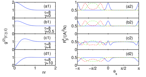
Figure 1: (color online). Density-density correlation function (LH column) and corresponding scattered intensity quadrature noise (RH column). Sequence shows transition from a decoherent classical gas to a high temperature Tonks gas. Incident angle $\theta_{\rm L}=0$ (solid blue lines); $\pi/4$ (red dashed lines); $\pi/2$ (green dot-dashed lines). Other parameters $({\bf k}_{\rm L})_{\rm x}=20n$, and $L\gg l_{c}$.

For weak interaction $g^{(2)}$ displays a peak at $r\approx 0$; thermal bunching. As $\gamma$ increases, the peak in $g^{(2)}$ changes to a dip; antibunching. The behaviour of the corresponding scattered intensity fluctuations, which consist of a noise floor ($|A|^{2}N/2$), plus the Fourier transform of $\eta=g^{(2)}-1$, can be readily understood. A positive (negative) function $\eta$ produces a peak (trough) in $R_{\frac{\pi}{4}}^{{\bf k}}$, with a width scaling inversely to $l_{c}$. This is clearly illustrated in the sequence of plots for $\theta_{\rm L}=0$ in Fig. 1. Atom bunching produces enhanced intensity fluctuations over a range of angles around $\theta_{s}=0$, while antibunching results in noise suppression in the scattered light over a similar angular range. We can interpret the more complex structure in Fig 1 (c2) as being due to a remnant bunching on a long spatial scale superimposed on a more dominant (and spatially narrower) antibunching. For an incident angle of $\pi/4$, these features are replicated around a (broader) transmitted peak at $\theta_{s}=-\pi/4$ and a reflected peak at $-3\pi/4$.

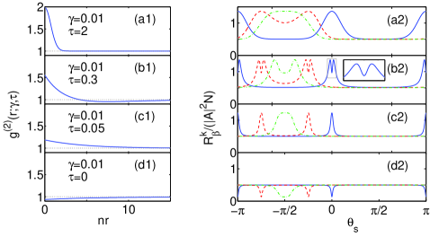
Figure 2: (color online). Density-density correlation function and scattered intensity quadrature noise for the transition from a decoherent classical gas to a zero temperature quasicondensate. Incident angle $\theta_{\rm L}=0$ (solid blue lines); $=\pi/4$ (red dashed lines); $=\pi/2$ (green dot-dashed lines). $({\bf k}_{\rm L})_{\rm x}=5n$, and $L\gg l_{c}$.

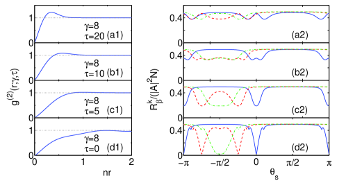
Figure 3: (color online). Density-density correlation function and scattered intensity quadrature noise for the transition from a high temperature Tonks gas to a low temperature Tonks gas. Incident angle $\theta_{\rm L}=0$ (solid blue lines); $=\pi/4$ (red dashed lines); $=\pi/2$ (green dot-dashed lines). $({\bf k}_{\rm L})_{\rm x}=20n$, $L\gg l_{c}$.

Fig. 2, where all plots are at weak interaction strength $\gamma=0.01$, shows the transition from a decoherent classical gas to a zero temperature quasicondensate as temperature is decreased to zero. At the higher temperatures, the scattered intensity fluctuations are enhanced in a broad angular region around the transmitted (and reflected) beams. At the lowest temperature, where $g^{(2)}$ displays weak antibunching with $l_{s}$ given by the condensate healing length (which is long), the light fluctuations are suppressed over a narrow angular range. Fig. 2(b1) exhibits competition between bunching and antibunching on different length scales, resulting in a subtle minima in $g^{(2)}$ at $nr\approx\tau/(4\gamma)$. This leads to a sharp dip in the noise features Fig. 2(b2) showing that light scattering is an ideal probe of these subtle, and controversial correlations2 , density-density correlations. Finally, in Fig. 3, a sequence of plots at constant large interaction strength $\gamma=8$, shows the transition from a high temperature to low temperature Tonks gas. In our analysis we have assumed the atoms are in an equilibrium state unperturbed by the interaction with the light. This assumption is valid provided the heating per atom from the recoil energy is much less than the initial energy per atom, $E_{0}$. The recoil component perpendicular to the trap axis is absorbed by the trap as a whole (because it is very tight), and so for $\theta_{\rm L}=0$, only the incoherently scattered light contributes to the heating. We can estimate the heating rate per atom to be $\Upsilon\hbar^{2}\langle k_{x}\rangle^{2}/2m$ where $\langle k_{x}\rangle^{2}$ is the mean square recoil momentum and $\Upsilon=\Gamma(\frac{\Omega_{\rm L}}{2\Delta_{\rm L}})^{2}$ is the rate of photon scattering CohenT . The perturbation to the initial state of the gas will be negligible provided $\Upsilon t\ll E_{0}$. Expressions for $E_{0}$ can be found from liebliniger .

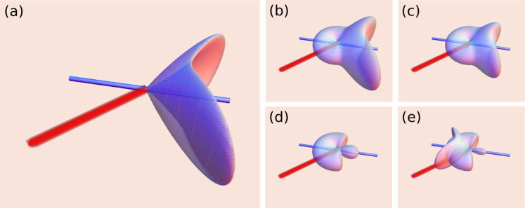
Figure 4: Intensity isosurfaces for coherently and incoherently scattered light. In each of the above figures, the blue cylinder shows the orientation of the 1D Bose gas, the red cylinder shows the direction of the incoming laser beam, and the semi-opaque, purple surface shows an intensity isosurface as a function of scattering angle. In (a) we show the intensity of the coherently scattered light [given by Eq. (5) in the main text] with $N^{2}\left(\frac{\Omega_{\rm L}}{2\Delta_{\rm L}}\right)^{2}\Gamma\hbar\omega_{\rm L}\frac{3}{8\pi r^{2}}=1$, $k_{\rm Lx}=0.7k_{\rm L}$ and $k_{\rm L}L\approx 28$. In (b)–(e) we show the incoherent intensity [given by Eq. (8) in the main text], for the approximation $\eta(r)=\eta e^{-r^{2}/(2l_{c}^{2})}$, with $N\left(\frac{\Omega_{\rm L}}{2\Delta_{\rm L}}\right)^{2}\Gamma\hbar\omega_{\rm L}\frac{3}{8\pi r^{2}}=1$, $k_{\rm Lx}=0.7k_{\rm L}$, $nl_{c}=1$ and $k_{\rm L}l_{c}=7$. In (b) we have $\eta=0.5$; in (c), $\eta=0.3$; in (d), $\eta=-0.3$; and in (e), $\eta=-1$.

In summary, we have shown that the quantum state of a 1D Bose gas can be nondestructively measured using off resonant light scattering. The angular distribution of the quadrature noise in the scattered light provides a direct signature of the nonlocal two-body correlations which characterize different system states of the gas. The method is useful across the full range of temperatures and atomic interaction strengths, and is capable of revealing subtle features in the density fluctuations that occur across multiple length scales. In addition, the method could also be used to monitor the dynamics of two-body correlations in the system, by simply solving the inverse Fourier transform of the intensity fluctuations.

This work was supported by the New Zealand Foundation for Research, Science and Technology under Contract No. NERF-UOOX0703. AGS gratefully acknowledges the support of the U.S. Department of Energy through the LANL/LDRD Program for this work.

References

- (1) W. Ketterle, D. S. Durfee, and D. M. Stamper-Kurn, in Proceedings of the International School of Physics Enrico Fermi, Course CXL, edited by M. Inguscio, S. Stringari, and C. E. Wieman, Bose-Einstein Condensation in Atomic Gases, (IOS Press, Amsterdam, 1999).
- (2) Juha Javanainen and Janne Ruostekoski, Phys. Rev. A 52, 3033 (1995).
- (3) S. Inouye, et al., Science 285, 571, (1999); J. Stenger, et al., Phys. Rev. Lett. 82, 4569, (1999).
- (4) Igor B. Mekhov, Christoph Maschler, and Helmut Ritsch, Phys. Rev. Lett. 98, 100402 (2007); Nat. Phys. 3, 319 (2007); Phys. Rev. A 76, 053618 (2007).
- (5) E. H. Lieb and W. Liniger, Phys. Rev. 130, 1605 (1963).
- (6) T. Cheon and T. Shigehara, Phys. Rev. Lett. 82, 2536 (1999).
- (7) A. G. Izergin, V. E. Korepin, and N. Y. Reshetikhin, J. Phys. A: Math. Gen. 20, 4799 (1987); D. M. Gangardt and G. V. Shlyapnikov, New J. Phys. 5, 79 (2003); K. V. Kheruntsyan, D. M. Gangardt, P. D. Drummond, and G. V. Shlyapnikov, Phys. Rev. Lett. 91, 040403 (2003); A. Y. Cherny and J. Brand, Phys. Rev. A 79, 043607 (2009).
- (8) A. Gorlitz, et al., Phys. Rev. Lett. 87, 130402 (2001); F. Schreck, et al., ibid. 87, 080403 (2001); M. Greiner, et al., ibid. 87, 160405 (2001). H. Moritz, T. Stöferle, M. Köhl, and T. Esslinger, ibid. 91, 250402 (2003); T. P. Meyrath, et al., Phys. Rev. A 71, 041604 (2005); T. Kinoshita, T. Wenger, and D. S. Weiss, Science 305, 1125 (2004); E. Haller, et al., Science 325, 1224(2009); E. Haller, et al., Nature 466, 597 (2010).
- (9) J. Armijo, T. Jacqmin, K. V. Kheruntsyan, and I. Bouchoule, Phys. Rev. Lett. 105, 230402 (2010); Thibaut Jacqmin, et al., ibid. 106, 230405 (2011);
- (10) Ehud Altman, Eugene Demler, and Mikhail D. Lukin, Phys. Rev. A 70, 013603, (2004); M. Greiner, C. A. Regal, J. T. Stewart, and D. S. Jin, Phys. Rev. Lett. 94,110401, (2005)
- (11) P. Deuar, et al., Phys. Rev. A 79, 043619 (2009); A. G. Sykes, et al., Phys. Rev. Lett. 100, 160406 (2008).
- (12) V. N. Popov, Functional Integrals in Quantum Field Theory and Statistical Physics (D. Reidel Pub., Dordrecht, 1983); D. S. Petrov, D. M. Gangardt, and G. V. Shlyapnikov, J. Phys. IV France 1, 1 (2007).
- (13) C. Cohen-Tannoudji, in Fundamental Systems in Quantum Optics, edited by J. Dalibard, et al., Atomic motion in laser light, (Elsevier Science, Amsterdam 1992).