Approximation of Löwdin Orthogonalization to a Spectrally Efficient Orthogonal Overlapping PPM Design for UWB Impulse Radio

Abstract

In this paper we consider the design of spectrally efficient time-limited pulses for ultra-wideband (UWB) systems using an overlapping pulse position modulation scheme. For this we investigate an orthogonalization method, which was developed in 1950 by Löwdin [1, 2]. Our objective is to obtain a set of $N$ orthogonal (Löwdin) pulses, which remain time-limited and spectrally efficient for UWB systems, from a set of $N$ equidistant translates of a time-limited optimal spectral designed UWB pulse. We derive an approximate Löwdin orthogonalization (ALO) by using circulant approximations for the Gram matrix to obtain a practical filter implementation as a tapped-delay-line [7]. We show that the centered ALO and Löwdin pulses converge pointwise to the same square-root Nyquist pulse as $N$ tends to infinity. The set of translates of the square-root Nyquist pulse forms an orthonormal basis for the shift-invariant-space generated by the initial spectral optimal pulse. The ALO transformation provides a closed-form approximation of the Löwdin transformation, which can be implemented in an analog fashion without the need of analog to digital conversions. Furthermore, we investigate the interplay between the optimization and the orthogonalization procedure by using methods from the theory of shift-invariant-spaces. Finally we relate our results to wavelet and frame theory.

1 Introduction

We consider in this work high data rate transmission in the ultra wideband (UWB) regime. To prevent disturbance of existing systems, e.g. GPS and UMTS, the Federal Communications Commission (FCC) released [5] a very low power spectral density (PSD) mask for ultra-wideband (UWB) systems. To ensure that sufficiently high signal-to-noise ratio (SNR) is maintained in the frequency band $F=[0,14]$GHz, as required by the FCC, the pulses have to be designed for a high efficient frequency utilisation. This utilisation can be expressed by the pulses normalized effective signal power (NESP) [6]. Several pulse shaping methods for pulse amplitude and pulse position modulation (PAM and PPM) were developed in the last decade based on a FIR prefiltering of a fixed basic pulse. Due to the high sampling rates in UWB this FIR filtering is realized by a tapped delay line [9]. A SNR optimization under the FCC mask constraints then reduces to a FIR filter optimization [7, 8, 6, 9].

Since the SNR is limited, the amount of signals can be increased to achieve higher data rates or to enable multi-user capabilities. For coherent and synchronized transmission over memoryless AWGN channels, an increased number $N$ of mutually orthogonal UWB signals inside the same time slot, known as $N$-ary orthogonal signal design, improves the BER performance over $E_{b}/N_{0}$ and hence the achievable rate of the system [10, Ch.4].

Combining spectral shaping and orthogonalization is an inherently difficult problem being neither linear nor convex. Therefore most methods approach this problem sequentially, e.g. combining spectral optimization with a Gram-Schmidt construction [11, 9, 12]. This usually results in an unacceptable loss in the NESP value of the pulses [13, 14]. Moreover these orthogonal pulses are different in shape and therefore not useful for PPM. Furthermore, a big challenge in UWB impulse radio (UWB-IR) implementation are high rate sampling operations. Therefore, an analog transmission scheme is desirable [15, 16, 14] to avoid high sampling rates in AD/DA conversion [15].

Usually, PPM is referred to an orthogonal (non-overlapping) pulse modulation scheme. To achieve higher data rates in PPM, pulse overlapping was already investigated in optical communication [17] and called OPPM. An application to UWB was studied for the binary case with a Gaussian monocycle [18]. To the authors’ knowledge, no orthogonal overlapping PPM (OOPPM) signaling has been considered based on strictly time-limited pulses. In this work we propose a new analog pulse shape design for UWB-IR to enable an almost OOPPM signaling which approximate the OOPPM scheme up to a desired accuracy.

In our approach, we first design a time-limited spectral optimized pulse $p$ and perform afterwards a Löwdin orthogonalization of the set of $2M\!+\!1$ integer translates $\{p(\cdot\!-\!k)\}_{k=-M}^{M}$, which span the function space $V^{M}(p)$. This orthogonalization method provides an implementable and stable approximation $p^{\circ,M}$ to a normalized square-root Nyquist pulse $p^{\circ}$ (all integer translates are mutually orthonormal) . Using the Fourier transformation for $p$ given by $\hat{p}(\nu)=\int_{\mathbb{R}}p(t)e^{-i2\pi t\nu}dt$ for every $\nu\in{\mathbb{R}}$, the square-root Nyquist pulse $p^{\circ}$ can be expressed in the frequency-domain

$$\hat{p}^{\circ}(\nu)=\frac{\hat{p}(\nu)}{\sqrt{\sum_{k}\left|\hat{p}(\nu-k)\right|^{2}}}$$ (1)

for $\nu$ almost everywhere, which is known as the orthogonalization trick [19].

Usually in digital signal processing, see Fig. 1, the time-continuous signals (pulses) in $L^{2}$ are sampled by an analog to digital (AD) operation (either in time or frequency) to obtain time-discrete signals in ${\mathbb{C}}^{2M+1}$. Then a discretization of the orthogonalization in (1) yields a finite digital transformation $D^{M}$ to construct a discrete signal in the frequency domain which has again to be transformed by a DA operation to obtain finally an approximation of the square-root Nyquist pulse [20].
Instead of using such an AD/DA conversion to operate in a discrete domain (depictured in Fig. 1 by the digital box), we use the democratic Löwdin orthogonalization $B^{M}$ (in the analog box), found by Per-Olov Löwdin in [1, 2], where all $2M+1$ linear independent pulse translates are involved simultaneously by a linear combination to generate a set of time-limited mutual orthonormal pulses. Hence the Löwdin orthogonalization is order independent. The Löwdin pulses constitute then an orthonormal basis for the span $V^{M}(p)$ of the initial basis $\{p(\cdot-k)\}_{k=-M}^{M}$. Moreover, as we will show in our main Theorem 2, the Löwdin orthogonalization $B^{M}$ is a stable approximation method to the construction in (1) and operates completely in the analog domain. Note, that a discretization of (1) generates neither shift-orthonormal pulses nor a set of mutual orthonormal pulses. The important property of the Löwdin method is its minimal summed energy distortion to the initial basis. It turns out that all orthonormal pulses maintain the spectral efficiency ”quite well”.

As $M$ tends to infinity the Löwdin orthogonalization $B=B^{\infty}$ applied to the initial pulse $p$ delivers the square-root Nyquist pulse $p^{\circ}$, which allows a real-time OOPPM system with only one single matched filter at the receiver. Since the Löwdin transform $B^{M}$ is hard to compute and to control we introduce an approximate Löwdin orthogonalization (ALO) $\tilde{B}^{M}$ and investigate its stability and convergence properties. It turns out that for fixed $M$ the transformations $B^{M}$ and $\tilde{B}^{M}$ are both implementable by a FIR filter bank (realised as a tapped delay line) like the spectral optimization in [9]. We call $B^{M}p$ and $\tilde{B}^{M}p\$ approximate square-root Nyquist pulses, since we observed that even for finite $M$ our analog approximation yields time–limited pulses with almost shift–orthogonal character since the sample values of the autocorrelation are below a measurable magnitude for the correlator. Hence such a construction of approximate square-root Nyquist pulses seems to be promising for an OOPPM system.

Figure 1: Analog and discrete approximation methods in time and frequency domains

The structure of this paper is as follows: In Section 2 we introduce the signal model and motivate our spectrally efficient $N$-ary orthogonal overlapping PPM design for UWB systems. Section 3 presents the state of the art in FCC optimal pulse shaping for UWB-IR based on PPM or PAM transmission by FIR prefiltering of Gaussian monocycles which is a necessary prerequisite for our design. To develop our approximation and convergence results in Section 4 we introduce the theory of shift–invariant spaces in Section 4.1 and in Section 4.2 the Löwdin orthogonalization for a set of $N$ translates to provide a $N$-ary orthogonal overlapping transmission. Our main result is given in Section 4.3, where we consider the stability of the Löwdin orthogonalization $B^{M}$ (for $M$ increasing to infinity) and develop for this a simplified approximation method $\tilde{B}^{M}$, called ALO. In Section 5 we study certain properties of our filter design and investigate the combination of both approaches. Furthermore, in Section 5.1 we develop a connection between our result and the canonical tight frame construction. Finally in Section 6, we demonstrate that the ALO and Löwdin transforms yields for sufficiently large filter orders compactly supported approximate square-root Nyquist pulses, which can be used for OOPPM having high spectral efficiency in the FCC region. Moreover, the Löwdin pulses provides also a spectrally efficient $(2M+1)$-ary orthogonal pulse shape modulation (PSM) [21].

2 Signal Model

In this work we will consider finite energy pulses $p$, i.e. the set $L^{2}:=\left\{\left.p:{\mathbb{R}}\to{\mathbb{C}}\rule[-2.5pt]{0.0pt}{10.0pt}\;\right|\;\left\|p\right\|_{L^{2}}<\infty\right\}$ of square-integrable functions with norm $\left\|\cdot\right\|_{L^{2}}:=\sqrt{\langle\cdot,\cdot\rangle}$ induced by the inner product

$$\langle p,q\rangle:=\int_{\mathbb{R}}p(t){\overline{q(t}})dt.$$ (2)

To control signal power in time or frequency locally we need pulses in $L^{\infty}:=\left\{\left.p:{\mathbb{R}}\to{\mathbb{C}}\rule[-2.5pt]{0.0pt}{10.0pt}\;\right|\;\left\|p\right\|_{\infty}<\infty\right\}$ which are essentially bounded, i.e. functions with a finite $L^{\infty}$-norm, given as

$$\left\|p\right\|_{\infty}:=\underset{t\in{\mathbb{R}}}{\operatorname{ess\,sup}}\left\{|p(t)|\right\},$$ (3)

where the essential supremum is defined as the smallest upper bound for $\left|p(t)\right|$ except on a set of measure zero. If the pulse is continuous than this implies boundedness everywhere. UWB-IR technology uses ultra short pulses, i.e. strictly time-limited pulses with support contained in a finite interval $X\subset{\mathbb{R}}$. We call such $L^{2}$- functions compactly supported in $X$ and denote its closed span by the subspace $L^{2}(X)$. The coding of an information sequence $\{d_{n}\}=\{d_{n}\}_{n\in{\mathbb{Z}}}$ is realized by pulse modulation techniques [12, 22] of a fixed normalized basic pulse $p\in L^{2}([0,T_{p}])$ with duration $T_{p}$.

A relevant issue in the UWB-IR framework and in our paper is the spectral shape of the pulse. In this section we will therefore summarize the derivation of spectral densities for common UWB modulation schemes such as PAM [7], PPM [23, 6, 24, 25, 26] and combinations of both [27] to justify our spectral shaping in the next section. Antipodal PAM and $N$-ary PPM are linear modulation schemes which map each data symbol $d_{n}$ to a pulse (symbol) $s_{d_{n}}(t)$ with the same power spectrum ${\mathcal{E}}\left|\hat{p}(\nu)\right|^{2}$. If we fix the energy ${\mathcal{E}}$ of the transmitted symbols and the pulse repetition time (symbol duration) $T_{s}$, we will show now for certain discrete random processes ( e.g. i.i.d. processes [3]) that the power spectrum density (PSD) of the transmitted signals is given by

$$S_{u}(\nu)=\frac{{\mathcal{E}}\left|\hat{p}(\nu)\right|^{2}}{T_{s}}.$$ (4)

Hence an optimization of the pulse power spectrum to the FCC mask $S_{\!F}(\nu)$ over the band $F$ in Section 3 increases the transmit power. To be more precise, PPM produces discrete spectral lines, induced by the periodic pulse repetition, the use of uniformly distributed pseudo-random time hopping (TH) codes $c_{n}\in[0,N_{c}]$ was suggested to reduce this effect and to enable multi-user capabilities [23, 25, 24, 28, 29]:

$$u(t)=\sum_{n=-\infty}^{\infty}\sqrt{{\mathcal{E}}}p(t-nT_{f}-c_{n}T_{c}-d_{\lfloor n/N_{f}\rfloor}T).$$ (5)

In [28] this is called framed TH by a random sequence, since the coding is repeated in each frame $N_{f}$ times with a clock rate of $1/T_{f}$. Hence $N_{f}T_{f}=T_{s}$ is the symbol duration for transmitting one out of $N$ symbol waveforms representing the encoded information symbol $d_{n}\in\{0,\dots,N-1\}$. To prevent ISI and collision with other users, the maximal PPM shift $T$ and TH shift $T_{c}$ have to fulfill $NT\leq T_{c}$ and $N_{c}T_{c}\leq T_{f}$. To ensure mutual orthogonality of all symbols one requires $T>T_{p}$. The PSD for independent discrete i.i.d. processes $\{c_{n}\},\{d_{n}\}$ follows from the Wiener-Khintchine Theorem [28, 30] to [6, (5)], [27, 31].

$$S_{u}(\nu)=\frac{{\mathcal{E}}\left|\hat{p}(\nu)\right|^{2}}{T_{f}}\left[1\!-\!\left|G_{\beta}(\nu)\right|^{2}+\frac{\left|G_{\beta}(\nu)\right|^{2}}{T_{f}}\sum_{k}\delta\left(\nu\!-\!\frac{k}{T_{f}}\right)\right]$$ (6)

$$\text{with }\left|G_{\beta}(\nu)\right|=\frac{1}{N_{c}N}\left|\frac{\sin(\pi\nu T_{c}N_{c})}{\sin(\pi\nu T_{c})}\right|\left|\frac{\sin(\pi\nu TN)}{\sin(\pi\nu T)}\right|\text{ and $\delta$ is the Dirac distribution}.$$ (7)

However, a more effective and simple reduction method without the use of frame repetition ($N_{f}=1$) or random TH ($N_{c}=1$) has been proposed in [27, 31]. Here antipodal PAM with $a_{n}\in\{-1,1\}$ is combined with $N$-ary PPM modulation, for $NT\leq T_{s}$

$$u(t)=\sqrt{{\mathcal{E}}}\sum_{n}a_{n}p(t-nT_{s}-d_{n}T).$$ (8)

The PSD for such i.i.d. processes is well known [22, Sec.4.3]:

$$S_{u}(\nu)=\frac{{\mathcal{E}}\left|\hat{p}(\nu)\right|^{2}}{T_{s}}\Bigg{[}{\mathbb{E}\left[a^{2}\right]}-\left|{\mathbb{E}\left[a\right]}\cdot{\mathbb{E}\left[e^{-i2\pi\nu dT}\right]}\right|^{2}+\frac{\left|{\mathbb{E}\left[a\right]}\cdot{\mathbb{E}\left[e^{-i2\pi\nu dT}\right]}\right|^{2}}{T_{s}}\sum_{n}\delta\left(\nu-\frac{n}{T_{s}}\right)\Bigg{]}\ ,$$ (9)

since we have $G_{\beta}(\nu)={\mathbb{E}\left[a\right]}{\mathbb{E}\left[e^{i2\pi\nu dT}\right]}$ in (7). For an i.i.d. process $\{a_{n}\}$ with expectation ${\mathbb{E}\left[a\right]}=0$ and variance ${\mathbb{E}\left[a^{2}\right]}=1$ the PSD reduces to (4). Hence the effective radiation power is essentially determined by the pulse shape times the energy ${\mathcal{E}}$ per symbol duration $T_{s}$ and should be bounded pointwise on $F$ below the FCC mask $S_{\!F}$

$$S_{u}(\nu)={\mathcal{E}}\frac{\left|\hat{p}(\nu)\right|^{2}}{T_{s}}\leq S_{\!F}(\nu)\quad\text{for all}\quad\nu\in F.$$ (10)

The optimal receiver for $N$-ary orthogonal PPM in a memoryless AWGN channel with noise power density ${\mathcal{N}_{0}}$ is the coherent correlation receiver. The uncoded bit rate $R_{b}$ and average symbol error probability $P_{s}$ is given as [10, 4.1.4]

$$R_{b}=\frac{\log{N}}{T_{s}}\quad\text{and}\quad P_{s}({\mathcal{E}})\leq(N-1)\operatorname{erfc}\left(\sqrt{\frac{{\mathcal{E}}}{{\mathcal{N}_{0}}}}\right),$$ (11)

where $\operatorname{erfc}$ is the complementary error function. Hence, a performance gain for fixed $T_{s}$ is achieved by increasing $N$ and/or ${\mathcal{E}}$.

Increasing $N$

Usually non–overlapping pulses are necessary in PPM to guarantee orthogonality of the set $\{p(\cdot-nT)\}:=\{p(\cdot-nT)\}_{n\in{\mathbb{Z}}}$ of pulse translates, i.e. $T>T_{p}$. For fixed $T_{p}$ this limits the number of pulses $N$ in $[0,T_{s}]$ and hence the rate $R_{b}$. In this work we will design an orthogonal overlapping PPM (OOPPM) system by keeping all overlapping translates mutually orthogonal. But such square-root Nyquist pulses are in general not time–limited, i.e. not compactly supported. In fact, we will show that for a particular class of compactly supported pulses a non-overlapping of the translates is necessary to obtain strict shift-orthogonality. However, we derive overlapping compactly supported pulses approximating the square-root Nyquist pulse in (1) and characterize the convergence. These approximations to the square-root Nyquist pulse allow a realizable $N$-ary OPPM implementation based on FIR filtering of time–limited analog pulses.

Increasing $\mathcal{E}$

The maximization of ${\mathcal{E}}$ with respect to the FCC mask was already studied in [6, 7] where a FIR prefiltering is used to shape the pulse such that its radiated power spectrum efficiently exploits and strictly respect the FCC mask. Note that the FCC regulation in (10) is a local constraint and does not force a strict band-limited design, however fast frequency decay outside the interval $F$ is desirable for a hardware realization.

Our combined approach now relies on the construction of two prefiltering operations to shape a fixed initial pulse. The first filter shapes the pulse to optimally exploit the FCC mask and the second filter generates an approximation to the square-root Nyquist pulse. The filter operations can be described as semi–discrete convolutions of pulses $p\!\in\!L^{2}$ with sequences ${\mathbf{c}}\in\ell^{2}:=\{{\mathbf{a}}\mid\left\|{\mathbf{a}}\right\|^{2}_{\ell^{2}}\!=\!\sum_{n}\left|a_{n}\right|^{2}\!<\!\infty\}$

$$p{\ *^{\prime}_{T}\,}{\mathbf{c}}:=\sum_{n\in{\mathbb{Z}}}c_{n}p(\cdot-nT),$$ (12)

at clock rate $1/T$. If we restrict ourselves to FIR filters of order $L$ the impulse response becomes a sequence ${\mathbf{c}}\in\ell^{2}(L)$ which can be regarded as a vectors in ${\mathbb{C}}^{L}$. Hence we refer for ${\mathbf{c}}\in{\mathbb{C}}^{L}$ to FIR filters and for ${\mathbf{c}}\in\ell^{2}$ to IIR filters.

3 FCC Optimization of a Single Pulse

The first prefilter operation generates an optimized FCC pulse $p$. To generate a time-limited real-valued pulse we consider a real-valued initial input pulse $q\in L^{2}([-T_{q}/2,T_{q}/2])$ and a real-valued (causal) FIR filter ${\mathbf{g}}\in{\mathbb{R}}^{L}$. A common UWB pulse is the truncated Gaussian monocycle $q$ [6, 7, 32], see also Section 6. The prefilter operation is then:

$$p(t)=(q{\ *^{\prime}_{T_{0}}\,}{\mathbf{g}})(t)=\sum_{k=0}^{L-1}g_{k}q(t-kT_{0})$$ (13)

which results in a maximal duration (support length) $T_{p}=(L-1)T_{0}+T_{q}$ of $p$.

To maximize the PSD according to (10) we have to shape the initial pulse by the filter ${\mathbf{g}}$ to exploit efficiently the FCC mask $S_{\!F}$ in the passband $F_{p}\!\subset\!F$, i.e. to maximize the ratio of the pulse power in $F_{p}$ and the maximal power allowed by the FCC

$$\eta(p):=\int_{F_{p}}|\hat{p}(\nu)|^{2}d\nu\bigg{/}\int_{F_{p}}S_{\!F}(\nu)d\nu.$$ (14)

This is known as the direct maximization of the NESP value $\eta(p)$, see [9]. Here we already included the constants ${\mathcal{E}}$ and $T_{s}$ in the basic pulse $p$. If we fix the initial pulse $q$, the clock rate $1/T_{0}$ and the filter order $L$, we get the following optimization problem

$$\begin{split}&\max_{{\mathbf{g}}\in{\mathbb{R}}^{L}}\tilde{\eta}\left(q{\ *^{\prime}_{T_{0}}\,}{\mathbf{g}}\right)\\ \text{s.t. }&\forall\nu\in F:\left|{\hat{\mathbf{g}}}(\nu)\right|^{2}\cdot\left|\hat{q}(\nu)\right|^{2}\leq S_{\!F}(\nu),\end{split}$$ (15)

where ${\hat{\mathbf{g}}}$ denotes the $1/T_{0}$ periodic Fourier series of ${\mathbf{g}}$, which is defined for an arbitrary sequence ${\mathbf{c}}\in\ell^{2}$ as

$$\hat{{\mathbf{c}}}(\nu)=\sum_{n=-\infty}^{\infty}c_{n}e^{-2\pi i\nu nT_{0}}.$$ (16)

Since ${\mathbf{g}}\in\ell^{2}(L)$ the sum in (16) becomes finite for ${\hat{\mathbf{g}}}$. Liu and Wan [33] studied the non-convex optimization problem (15) with non-linear constraints numerically with fmincon, a Matlab program. The disadvantage of this approach lies in the trap of a local optimum, which can only be overcome by an intelligent choice of the start parameters.

Alternatively (15) can be reformulated in a convex form by using the Fourier series of the autocorrelation $r_{{\mathbf{g}},n}:=\sum_{k}g_{k}g_{k-n}$ of the filter ${\mathbf{g}}$ [34]. Since $r_{{\mathbf{g}},n}=r_{{\mathbf{g}},-n}$ (real-valued symmetric sequence) we write

$${\hat{\mathbf{r}}_{{\mathbf{g}}}}(\nu) :=\sum_{n=0}^{L-1}r_{{\mathbf{g}},n}\phi_{n}(\nu)=\left|{\hat{\mathbf{g}}}(\nu)\right|^{2}$$ (17)

on the frequency band $[-\frac{1}{2T_{0}},\frac{1}{2T_{0}}]$ by using the basis $\boldsymbol{\phi}:=\left\{1,2\cos(2\pi\nu T_{0}),2\cos(2\pi\nu 2T_{0}),\dots\right\}$ and get $\left|\hat{p}(\nu)\right|^{2}={\hat{\mathbf{r}}_{{\mathbf{g}}}}(\nu)\cdot\left|\hat{q}(\nu)\right|^{2}$. Due to the symmetry of $\phi_{n}$ and $S_{\!F}$ we can restrict the constraints in (15) to $F=[0,\frac{1}{2T_{0}}]$ and obtain the following semi–infinite linear problem:

$$\max_{\mathbf{r}_{{\mathbf{g}}}\!\in{\mathbb{R}}^{L}}\sum_{n=0}^{L-1}r_{{\mathbf{g}},n}c_{n}\quad\!\text{such that}\quad 0\leq{\hat{\mathbf{r}}_{{\mathbf{g}}}}(\nu)\leq{\mathcal{M}}(\nu)\ \text{ for all $\ \nu\!\in\!\left[0,\frac{1}{2T_{0}}\right]$}$$ (18)

$$\text{with}\quad{\mathcal{M}}(\nu):=\frac{S_{\!F}(\nu)}{\left|\hat{q}(\nu)\right|^{2}}\quad\text{and}\quad c_{n}:=\int_{F_{p}}\left|\hat{q}(\nu)\right|^{2}\phi_{n}(\nu)d\nu.$$ (19)

Since the FCC mask is piecewise constant, we separate ${\mathcal{M}}(\nu)$ into five sections ${\mathcal{M}}_{i}(\nu)$ [35] and get the inequalities

$$\forall i={1,\dots,5}:\ {\hat{\mathbf{r}}_{{\mathbf{g}}}}(\nu) \leq{\mathcal{M}}_{i}(\nu)\quad\text{for}\quad\nu\in[\alpha_{i},\beta_{i}]$$ (20)

with $\beta_{1}=1.61,\beta_{2}=1.99,\beta_{3}=3.1,\beta_{4}=10.6,\beta_{5}=14$ and $\alpha_{1}=\alpha_{2}=\alpha_{3}=\alpha_{4}=0,\alpha_{5}=\beta_{4}$ in GHz, see Fig. 2.
The necessary lower bound for $\mathbf{r}_{{\mathbf{g}}}$ reads

$${\hat{\mathbf{r}}_{{\mathbf{g}}}}(\nu)\geq 0\quad\text{for}\quad\nu\in\left[0,\frac{1}{2T_{0}}\right]=[0,14]\text{GHz}.$$ (21)

To formulate the constraints in (19) for $\mathbf{r}_{{\mathbf{g}}}$ as a positive bounded cone in ${\mathbb{R}}^{L}$ we approximate ${\mathcal{M}}_{i}(\nu)$ by trigonometric polynomials $\Gamma_{i}(\nu):=\sum_{n}\gamma_{i,n}\phi_{n}(\nu)$ of order $L$ in the $L^{2}$-norm [35]. The semi-infinite linear constraints in (20) describe a compact convex set [34, (40),(41)]. To see this, let us introduce the following lower bound cones for $\theta\in[0,\frac{1}{2T_{0}}]$

$$K_{\text{low}}(\theta) =\left\{\mathbf{r}_{{\mathbf{g}}}\in{\mathbb{R}}^{L}\bigg{|}\sum_{k=0}^{L-1}r_{{\mathbf{g}},n}\phi_{n}(\nu)\geq 0,\nu\in\left[\theta,\frac{1}{2T_{0}}\right]\right\}.$$ (22)

For $\theta=0$ the positive cone $K_{0}=K_{\text{low}}(0)$ defines the lower bound in (21) if we set $T_{0}=\frac{1}{28\text{GHz}}$. To formulate the non-constant upper bounds, one can use the approximation functions $\Gamma_{i}(\nu)$ [35] given in the same basis $\boldsymbol{\phi}$ as $\left|{\hat{\mathbf{g}}}(\nu)\right|^{2}$. For each $i\in\{1,\dots,5\}$ the bounds in (20) are then equivalent to

$$\sum_{n=1}^{L}(\gamma_{i,n}-r_{{\mathbf{g}},n})\phi_{n}(\nu)\geq 0\quad\text{for}\quad\nu\in[\alpha_{i},\beta_{i}].$$ (23)

For the upper bounds, we just have to set $\rho_{i,n}:=\gamma_{i,n}-r_{{\mathbf{g}},n}$ for each $i=1,\dots,5$ and $n\geq 1$, which leads to the upper bound cones

$$K_{\text{up}}(\theta_{i}) =\bigg{\{}\mathbf{r}_{{\mathbf{g}}}\in{\mathbb{R}}^{L}\bigg{|}\sum_{n=0}^{L-1}\rho_{i,n}\phi_{n}(\nu)\geq 0,\nu\in\left[\theta_{i},\frac{1}{2T_{0}}\right]\bigg{\}},$$ (24)

$$\bar{K}_{\text{up}}(\theta_{i}) =\bigg{\{}\mathbf{r}_{{\mathbf{g}}}\in{\mathbb{R}}^{L}\bigg{|}\sum_{n=0}^{L-1}\rho_{i,n}\phi_{n}(\nu)\geq 0,\nu\in\left[0,\theta_{i}\right]\bigg{\}}.$$ (25)

The five upper bound cones $K_{i}$ are then

$$\forall i=1,\dots,4:\ K_{i} :=\bar{K}_{\text{up}}(\beta_{i})\quad\text{and}\quad K_{5}:={K}_{\text{up}}(\alpha_{5}).$$ (26)

Since the autocorrelation has to fulfill all these constraints, it has to be an element of the intersection. After this approximation we get from (15) the problem

$$\max_{\mathbf{r}_{{\mathbf{g}}}\in\bigcap_{i}K_{i}}\sum_{n=0}^{L-1}r_{{\mathbf{g}},n}c_{n}.$$ (27)

This is now a convex optimization problem of a linear functional over a convex set. By the positive real lemma [34], these cone constraints can be equivalently described by semi-positive-definite matrix equalities, s.t. the problem (27) is numerically solvable with the matlab toolbox SeDuMi [8, 36]. The filter is obtained by a spectral factorization of $r_{{\mathbf{g}}}$. Obviously ${\mathbf{g}}$ is not uniquely determined.

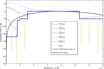
Figure 2: Fourier-approximations $\Gamma_{i}^{L}$ of $\mathcal{M}$ for $L=25$.

Note that this optimization problem can also be seen as the maximization of a local $L^{2}$-norm, given as the NESP value, under the constraints of local $L^{\infty}$-norms.

4 Orthogonalization of Pulse Translates

In [7, 14] a sequential pulse optimization was introduced, which produces mutually orthogonal pulses $p^{\circ}_{m}=q{\ *^{\prime}_{T_{0}}\,}{\mathbf{g}}_{m}$, i.e. $\langle p^{\circ}_{m},p^{\circ}_{n}\rangle=\delta_{nm}$. Here each pulse $p^{\circ}_{m}$ is generated by a different FIR filter ${\mathbf{g}}_{m}\in{\mathbb{R}}^{L}$, which depends on the previously generated pulses $p^{\circ}_{1},\dots,p^{\circ}_{m-1}$ and produces pulses in $L^{2}([-T_{q}/2,(L-1)T_{0}+T_{q}/2])$. This approach is similar to the Gram-Schmidt construction in that it is order-dependent, since the first pulse $p^{\circ}_{1}$ can be optimally designed to the FCC mask without an orthogonalization constraint. We will now present a new order–independent method to generate from a fixed initial pulse $p$ a set of orthogonal pulses $\{p^{\circ}_{m}\}$. Therefore we introduce a new time–shift $T>0$, namely the PPM shift in (5), to generate a set of $N=2M+1$ translates $\{p(\cdot-mT)\}_{m=-M}^{M}$, i.e. $M$ shifts in each time direction. The orthogonal pulses are then obtained by linear combinations of the translates of the initial pulse $p$. For a stable embedding of the finite construction we restrict the initial pulses to the set $L^{2}_{T_{p}}:=L^{2}([-T_{p}/2,T_{p}/2])$ of centered pulses with finite duration $T_{p}$. To study the convergence we need to introduce the concept of regular shift–invariant spaces.

4.1 Shift–Invariant Spaces and Riesz-Bases

To simplify notation we scale the time axis so that $T=1$. Let us now consider the set ${\mathcal{S}}_{0}(p):=\operatorname{span}\{p(\cdot-n)\}$ of all finite linear combinations of $\{p(\cdot-n)\}$, which is certainly a subset of $L^{2}$. The $L^{2}$-closure of ${\mathcal{S}}_{0}(p)$ is a shift–invariant closed subspace ${\mathcal{S}}(p):={\overline{{\mathcal{S}}_{0}(p)}}\subset L^{2}$, i.e. for each $f\in{\mathcal{S}}(p)$ also $\{f(\cdot-n)\}\subset{\mathcal{S}}(p)$. Since ${\mathcal{S}}(p)$ is generated by a single function $p$ we call it a principal shift–invariant (PSI) space and $p$ the generator for ${\mathcal{S}}(p)$. In fact, ${\mathcal{S}}(p)$ is the smallest PSI closed subspace of $L^{2}$ generated by $p$. Of course not every closed PSI space is of this form [37]. In this work we are interested in spaces which are closed under semi-discrete convolutions (12) with $\ell^{2}$ sequences, i.e. the space

$$V(p):=\left\{\left.p{\ *^{\prime}\,}{\mathbf{c}}\rule[-0.39098pt]{0.0pt}{9.13986pt}\;\right|\;{\mathbf{c}}\in\ell^{2}\right\}$$ (28)

endowed with the $L^{2}$- norm. Note that $V(p)$ is in general not a subspace or even a closed subspace of $L^{2}$ [37, 38]. But to guarantee stability of our filter design $V(p)$ has to be closed, i.e. has to be a Hilbert subspace. More precisely, the translates of $p$ have to form a Riesz basis.

Definition 1.

Let ${\mathcal{H}}$ be a Hilbert space. $\{e_{n}\}\subset{\mathcal{H}}$ is a Riesz basis for $\overline{\operatorname{span}\{e_{n}\}}$ if and only if there are constants $0<A\leq B<\infty$, s.t.

$$A\left\|{\mathbf{c}}\right\|^{2}_{\ell^{2}}\leq\left\|\sum_{n}c_{n}e_{n}\right\|^{2}_{{\mathcal{H}}}\leq B\left\|{\mathbf{c}}\right\|^{2}_{\ell^{2}}\quad\text{for all}\quad{\mathbf{c}}\in\ell^{2}.$$ (29)

In this case $\overline{\operatorname{span}\{e_{n}\}}$ becomes a Hilbert-subspace of ${\mathcal{H}}$. For SI spaces in $L^{2}={\mathcal{H}}$ we get the following result.

Proposition 1 (Prop.1 in [39]).

Let $p\in L^{2}({\mathbb{R}})$.

Then $V(p)$ is a closed shift–invariant subspace of $L^{2}$ if and only if

$$A\left\|{\mathbf{c}}\right\|^{2}_{\ell^{2}}\leq\left\|p{\ *^{\prime}\,}{\mathbf{c}}\right\|^{2}_{L^{2}}\leq B\left\|{\mathbf{c}}\right\|^{2}_{\ell^{2}}\quad\text{for all}\quad{\mathbf{c}}\in\ell^{2}$$ (30)

holds for fixed constants $0<A\leq B<\infty$. Moreover, $\{p(\cdot-n)\}$ is a Riesz-basis for $V(p)$.

If the generator $p$ fulfills (30), then $V(p)={\mathcal{S}}(p)$ by [40] and we call $p$ a stable generator and $V(p)$ a regular PSI space [37]. An orthonormal generator (square-root Nyquist pulse, shift-orthonormal pulse) $p^{\circ}$ for $V(p)$ is a generator with $\langle p^{\circ}(\cdot-n),p^{\circ}(\cdot-m)\rangle=\delta_{mn}$ for all $n,m\in{\mathbb{Z}}$ [11, Lap09]. Benedetto and Li [41] showed that the stability and orthogonality of a generator $p\in L^{2}$ can be described by the absolute $[0,1]$-integrable periodic function $\Phi_{p}\in L^{1}([0,1])$ of $p$ defined for $\nu$ almost everywhere (a.e.) as

$$\Phi_{p}(\nu):=\sum_{k}\left|\hat{p}(\nu+k)\right|^{2}.$$ (31)

They could show the following characterization [42, 41].

Theorem 1 (Th. 7.2.3 in [42]).

A function $p\in L^{2}$ is a stable generator for $V(p)$ if and only if there exists $0<A\leq B<\infty$ such that

$$A\leq \Phi_{p}(\nu)\leq B\qquad\text{for $\nu$ a.e.}$$ (32)

and is an orthonormal generator for $V(p)$ if and only if

$$\Phi_{p}(\nu)=1\qquad\text{for $\nu$ a.e.. }$$ (33)

Proof.

For a proof see Th. 7.2.3. (ii) and (iii) in [42]. In our special case we have $B=1$. Note, that the Riesz sequence and orthonormal sequence are bases for their closed span, meaning that in our case ${\mathcal{S}}(p)=V(p)$. ∎

Due to this characterization in frequency there is a simple “orthogonalization trick” for a stable generator given in (1), which was found by Meyer, Mallat, Daubechies and others [43],[42, Prop. 7.3.9]. Unfortunately, this does not provide an “a priori” construction in the time domain and does not lead to a support control of the orthonormal generator in time, as necessary for UWB-IR.

Contrary to an approximation in the frequency-domain we approach an approximation in time-domain via the Löwdin transformation. We will show that in the limit the Löwdin transformation for shift–sequences is in fact given in frequency by the orthogonalization trick (1). By using finite section methods we establish an approximation method in terms of the discrete Fourier transform (DFT) to allow an easy computation. Furthermore, we show that the Löwdin construction for stable generators is unique and optimal in the $L^{2}$-distance among all orthonormal generators and corresponds to the canonical construction of so called tight frames (given later).

4.2 Löwdin Orthogonalization for Finite Dimensions

Since the Löwdin transformation is originally defined for a finite set of linearly independent elements in a Hilbert space ${\mathcal{H}}$, we will use the finite section method to derive a stable approximation to the infinite case. For this we consider for any $M\in{\mathbb{N}}$ the symmetric orthogonal projection $\mathbf{P}\!_{M}$ from $\ell^{2}$ to $\ell^{2}_{M}=\{{\mathbf{c}}\in\ell^{2}|\operatorname{supp}{\mathbf{c}}\!\subset\!\{-\!M,\dots,M\}\}$ defined for ${\mathbf{c}}\in\ell^{2}$ by $\mathbf{P}\!_{M}{\mathbf{c}}:={\mathbf{c}}^{M}=(0,\dots,0,c_{-M},\dots,c_{M},0,\dots,0)$. Then the finite section ${{\mathbf{G}}_{M}}$ of the infinite dimensional Gram matrix ${\mathbf{G}}$ of $p\in L^{2}$, given by

$$\left[{\mathbf{G}}\right]_{nm} :=\langle p(\cdot-m),p(\cdot-n)\rangle\quad\text{for}\quad n,m\in{\mathbb{Z}},$$ (34)

can be defined as ${{\mathbf{G}}_{M}}:=\mathbf{P}\!_{M}{\mathbf{G}}\mathbf{P}\!_{M}$, see [44, Prop. 5.1.5]. If $p$ satisfies (29) and if we restrict the semi-discrete convolution $p{\ *^{\prime}\,}{\mathbf{c}}$ to $\ell^{2}_{M}$, we obtain a $2M+1$ dimensional Hilbert subspace $V^{M}(p)$ of $V(p)={\mathcal{H}}$. Then the unique linear operation $B^{M}$, which generates from $\{p(\cdot-m)\}_{m=-M}^{M}$ an orthonormal basis (ONB) $\{p^{\circ,M}_{m}\}_{m=-M}^{M}$ for $V^{M}(p)$ and simultaneously minimizes

$$\sum_{m=-M}^{M}\left\|B^{M}p(\cdot-m)-p(\cdot-m)\right\|_{L^{2}}^{2}$$ (35)

is given by the (symmetric) Löwdin transformation [1, 2, 45, 46] and can be represented in matrix form as

$$p^{\circ,M}_{m}:=B^{M}p(\cdot-m)=\sum_{n=-M}^{M}[{\mathbf{G}_{M}^{-\frac{1}{2}}}]_{mn}p(\cdot-n)\quad\text{for all}\quad m\in\{-M,\dots,M\},$$ (36)

where we call each $p^{\circ,M}_{m}$ a Löwdin orthogonal (LO) pulse or Löwdin pulse.

Here ${\mathbf{G}_{M}^{-\frac{1}{2}}}$ denotes the (canonical) inverse square-root (restricted to $\ell^{2}_{M}$) of ${{\mathbf{G}}_{M}}$. Note that ${\mathbf{G}_{M}^{-\frac{1}{2}}}$ is not equal to $\mathbf{P}\!_{M}{\mathbf{G}^{-\frac{1}{2}}}\mathbf{P}\!_{M}$. Since the sum in (36) is finite, the definition of the Löwdin pulses is also pointwise well-defined. In the next section, we will see that this is a priori not true for the infinite case. If we identify the corresponding $m$’th row of the inverse square-root of ${{\mathbf{G}}_{M}}$ with vectors $\mathbf{b}^{M}_{m}=([{\mathbf{G}_{M}^{-\frac{1}{2}}}]_{m\,-\!M},\dots,[{\mathbf{G}_{M}^{-\frac{1}{2}}}]_{m\,+\!M})$ we can describe (36) by a FIR filter bank as

$${p^{\circ,M}_{m}}=p{\ *^{\prime}\,}\mathbf{b}^{M}_{m}\quad,\quad m\in\{-M,\dots,M\}.$$ (37)

Unfortunately, none of these Löwdin pulses is a shift-orthonormal pulse, which would be necessary for an OOPPM transmission. In the next section we will thus show that the Löwdin orthogonalization converges for $M$ to infinity to an IIR filter ${\mathbf{b}}$ given as the centered row of ${\mathbf{G}^{-\frac{1}{2}}}$. This IIR filter generates then a shift-orthonormal pulse, namely the square-root Nyquist pulse defined in (1). Hence the Löwdin orthogonalization (36) provides an approximation to our OOPPM design. In the following we will investigate its stability, i.e. its convergence property.

4.3 Stability and Approximation

In this section we investigate the limit of the Löwdin orthogonalization in (36) for translates (time-shifts) of the optimized pulse $p$ with time duration $T_{p}<\infty$ where we further assume that $p$ is a bounded stable generator. If we set $K:=\lfloor T_{p}\rfloor$ then certainly $p\in L^{2}_{K}$. In this case the auto–correlation of $p$

$$r_{p}(t):=(p*{\overline{p}}_{-})(t)=\int_{\mathbb{R}}p(\tau){\overline{p(\tau-t)}}d\tau,$$ (38)

with the time reversal $p_{-}(t):=p(-t)$ is a compactly supported bounded function on $[-K,K]$. Due to the Poisson summation formula we can represent $\Phi_{p}$ almost everywhere by the Fourier series (16) ($T_{0}=1$) of the samples $\{r_{p}(n)\}$

$$\Phi_{p}(\nu)=\sum_{n=-\infty}^{\infty}r_{p}(n)e^{-2\pi in\nu}=\sum_{n=-K}^{K}[{\mathbf{G}}]_{n0}e^{-2\pi in\nu},$$ (39)

which is the symbol of the Toeplitz matrix ${\mathbf{G}}$, since we have from (34) and (38) that $r_{p}(n-m)=[{\mathbf{G}}]_{nm}$. Moreover the symbol is continuous since the sum is finite due to the compactness of $r_{p}$.

On the other hand the initial pulse $p$ is a Wiener function [44, Def. 6.1.1] so that $\Phi_{p}$ defines a continuous function and condition (32) holds pointwise [47, Prop.1]. Since both sides in (39) are identical a.e. they are identical everywhere by continuity (see also [44, p.105]). Thus, the spectrum of ${\mathbf{G}}$ is continuous, strictly positive and bounded by the Riesz bounds. Hence the inverse square-roots of ${\mathbf{G}}$ and ${{\mathbf{G}}_{M}}$ exists s.t. for any $M\in{\mathbb{N}}$ (by Cauchy’s interlace theorem, [48, Th. 9.19])

$$A{\mathbf{1}}_{M}\leq{\mathbf{G}}_{M}\leq B{\mathbf{1}}_{M}\quad\text{and}\quad\frac{1}{B}{\mathbf{1}}_{M}\leq{\mathbf{G}^{-1}_{M}}\leq\frac{1}{A}{\mathbf{1}}_{M},$$ (40)

where ${\mathbf{1}}_{M}$ denotes the identity on $\ell^{2}_{M}$. Now we can approximate the Gram matrix by Strang’s circulant preconditioner [49], s.t. the diagonalization is given by a discrete Fourier transform (DFT) [50]. To get a continuous formulation of the approximated Löwdin pulses we use the Zak transform [51], given for a continuous function $f$ as

$$({\mathbf{Z}}f)(t,\nu):=\sum_{n\in{\mathbb{Z}}}f(t-n)e^{2\pi in\nu}\quad\text{for}\quad t,\nu\in{\mathbb{R}}.$$ (41)

Our main result is the following theorem.

Theorem 2.

Let $K\in{\mathbb{N}}$ and $p\in L^{2}_{K}$ be a continuous stable generator for $V(p)$. Then we can approximate the limit set of the Löwdin pulses $\{p^{\circ}_{m}\}$ by a sequence of finite function sets $\{\tilde{p}_{m}^{\circ,M}\}_{m=-M}^{M}$, which are approximate Löwdin orthogonal (ALO). The functions $\tilde{p}_{m}^{\circ,M}$ are given pointwise for $M\geq K$ and $m\in\{-M,\dots,M\}$ by the Zak transform as

$${{\tilde{p}}^{\circ,M}_{m}}\!(t)\!:=\!\begin{cases}\frac{1}{2M\!+\!1}\overset{2M}{\underset{{l=0}}{\sum}}\frac{e^{\frac{-2\pi iml}{2M+1}}({\mathbf{Z}}p)(t,\frac{l}{2M+1})}{\sqrt{({\mathbf{Z}}r_{p})(0,\frac{l}{2M+1})}}&\left|t\right|\!\leq\!M\!-\!\frac{K}{2}\\ 0&\text{else}\end{cases},$$ (42)

such that for each $m\in{\mathbb{Z}}$

$$\tilde{p}^{\circ}_{m}(t)=\lim_{M\to\infty}{{\tilde{p}}^{\circ,M}_{m}}(t)$$ (43)

converges pointwise on compact sets. The limit in (43) can be stated as

$$\hat{\tilde{p}}^{\circ}(\nu) =\hat{p}(\nu)\cdot\left(\Phi_{p}(\nu)\right)^{-\frac{1}{2}}$$ (44)

for $\nu\in{\mathbb{R}}$ in the frequency-domain. Hence the Löwdin generator $\tilde{p}^{\circ}:=\tilde{p}^{\circ}_{0}$ is an orthonormal generator for $V(p)$.

Proof.

The proof consists of two parts. In the first part we derive an straightforward finite construction in the time domain to obtain time-limited pulses (42) being approximations to the Löwdin pulses. Using Strang’s circulant preconditioner the ALO pulses can be easily derived in terms of DFTs. In the second part we will then show that this finite construction is indeed a stable approximation to the square-root Nyquist pulse. Here we need pointwise convergence, i.e. convergence in $\ell^{\infty}$ (the set of bounded sequences). Finally, to establish the shift-orthogonality we use properties of the Zak transform.

Since the inverse square-root of a $N\times N$ Toeplitz matrix is hard to compute, we approximate for any $M\geq K$ the Gram matrix ${{\mathbf{G}}_{M}}$ by using Strang’s circulant preconditioner ${{\mathbf{\tilde{G}}}_{M}}$ [49, 52]. Moreover, the Gram matrix is hermitian and banded such that we can define the elements of the first row by [53, (4.19)] as

$$[{{\mathbf{\tilde{G}}}_{M}}]_{0n}:=\begin{cases}r_{p}(n)&n\in\{0,\dots,K\}\\ r_{p}(N-n)&n\in\{N-K,\dots,N-1\}\\ 0&\text{else}\end{cases}.$$ (45)

Here we abbreviate $N:=2M+1$. The crucial property of Strang’s preconditioner ${{\mathbf{\tilde{G}}}_{M}}$ is the fact that the eigenvalues $\lambda_{l}({{\mathbf{\tilde{G}}}_{M}})$ are sample values of the symbol $\Phi_{p}$ in (31). This special property is in general not valid for other circulant preconditioners [52]. To see this, we derive the eigenvalues by [53, Theorem 7] as

$${\tilde{\lambda}}_{l}^{M}:=\lambda_{l}({{\mathbf{\tilde{G}}}_{M}}) =\sum_{n=0}^{K}r_{p}(n)e^{-2\pi in\frac{l}{N}}+\sum_{n=N-K}^{N-1}r_{p}(N-n)e^{-2\pi in\frac{l}{N}}\quad\text{for}\quad l\in\{0,\dots,2M\}$$ (46)

by inserting the first row of ${{\mathbf{\tilde{G}}}_{M}}$ given in (45). If we set in the second sum $n^{\prime}=n-N$ we get from (39)

$${\tilde{\lambda}}^{M}_{l} =\sum_{n=-K}^{K}r_{p}(n)e^{-2\pi il\frac{n}{N}}=\Phi_{p}\left(\frac{l}{2M+1}\right).$$ (47)

Since $p$ is compactly supported the symbol $\Phi_{p}$ is continuous and the second equality in (47) holds pointwise. Moreover, the Riesz bounds (32) of $p$ guarantee that ${{\mathbf{\tilde{G}}}_{M}}$ is strictly positive and invertible for any $M$. Now we are able to define the ALO pulses in matrix notation by setting in $\mathbf{p}^{M}(t):=\{p(t\!-\!n)\}_{n=-M}^{M}=(p(t\!+\!M),\dots,p(t\!-\!M))^{T}$ for any $t\in{\mathbb{R}}$

$${\tilde{\mathbf{p}}}^{\circ,M}(t):={\mathbf{\tilde{G}}_{M}^{-\frac{1}{2}}}\mathbf{p}^{M}(t) ={\mathbf{F}_{M}}{\mathbf{\tilde{D}}_{M}^{-\frac{1}{2}}}{\mathbf{F}_{M}^{*}}\mathbf{p}^{M}(t),$$ (48)

since the circulant matrix ${{\mathbf{\tilde{G}}}_{M}}={\mathbf{F}_{M}}{\tilde{{\mathbf{D}}}_{M}}{\mathbf{F}_{M}^{*}}$ can be written by the unitary $N\times N$ DFT matrix ${\mathbf{F}_{M}}$, with

$$[{\mathbf{F}_{M}}]_{nm}:=\frac{1}{\sqrt{N}}e^{-2\pi i\frac{nm}{N}}\quad\text{with}\quad n,m\!\in\!\{0,\dots,2M\}$$ (49)

and the diagonal matrix ${\tilde{{\mathbf{D}}}_{M}}$ of the eigenvalues of ${{\mathbf{\tilde{G}}}_{M}}$.

Let us start in (48) from the right by applying the IDFT matrix ${\mathbf{F}_{M}^{*}}$, then we get for any $k$th component with $k\in\{0,\dots,2M\}$

$$[{\mathbf{F}_{M}^{*}}\mathbf{p}^{M}(t)]_{k} =\frac{1}{\sqrt{N}}\Bigg{(}\sum_{n=0}^{M}e^{2\pi i\cdot\frac{n}{N}k}\cdot p(t+M-n)+\sum_{n=M+1}^{2M}e^{2\pi i\cdot\frac{n}{N}k}\cdot p(t+M-n)\Bigg{)}$$ (50)

$$\!\!\!\overset{\overset{j=n-M}{\downarrow}}{=}\frac{1}{\sqrt{N}}\sum_{j=-M}^{M}e^{2\pi i\cdot\frac{j+M}{N}k}\cdot p(t-j).$$ (51)

Next we multiply with the components $[{\mathbf{\tilde{D}}_{M}^{-\frac{1}{2}}}]_{kl}=\delta_{kl}/\sqrt{{\tilde{\lambda}}^{M}_{l}}$ of the inverse square-root of the diagonal matrix ${\tilde{{\mathbf{D}}}_{M}}$

$$\left[{\mathbf{\tilde{D}}_{M}^{-\frac{1}{2}}}{\mathbf{F}_{M}^{*}}\mathbf{p}^{M}(t)\right]_{l} =\frac{1}{\sqrt{N}}\sum_{j,k}\left(\frac{\delta_{kl}}{\sqrt{{\tilde{\lambda}}_{l}^{M}}}e^{2\pi i\frac{j+M}{N}k}\cdot p(t-j)\right)=\frac{1}{\sqrt{N}}\left(\sum_{j=-M}^{M}\frac{e^{2\pi i\frac{j+M}{N}l}\cdot p(t-j)}{\sqrt{{\tilde{\lambda}}^{M}_{l}}}\right).$$ (52)

In the last step we evaluate the DFT at $m\in\{0,\dots,2M\}$

$${{\tilde{p}}^{\circ,M}_{m\!-\!M}}(t)=[{\tilde{\mathbf{p}}}^{\circ,M}(t)]_{m} =\frac{1}{N}\sum_{l=0}^{2M}\left(\frac{e^{-2\pi im\cdot\frac{l}{N}}}{\sqrt{{\tilde{\lambda}}_{l}^{M}}}\sum_{j=-M}^{M}p(t-j)e^{2\pi il\frac{j+M}{N}}\right)=\frac{1}{N}\sum_{l=0}^{2M}e^{-2\pi il\frac{m-M}{N}}\frac{\sum_{j=-M}^{M}p(t-j)e^{2\pi il\cdot\frac{j}{N}}}{\sqrt{({\mathbf{Z}}r_{p})(0,\frac{l}{N})}}.$$ (53)

where we used the Zak transform (41) of $r_{p}$ to express the eigenvalues ${\tilde{\lambda}}^{M}_{l}$. In the next step we extend the DFT sum of the numerator in (53) to an infinite sum. This is possible since $p(\cdot-k)$ always has the same support length $K$ for each $k\in{\mathbb{Z}}$. Thus, for all $\left|t\right|>M-\frac{K}{2}$ the non-zero sample values are shifted in the kern of $\mathbf{P}_{M}$; hence $\mathbf{p}^{M}(t)=0$. On the other hand for $\left|t\right|\leq M-\frac{K}{2}$ any shift $\left|j\right|>M$ results in $p(t-j)=0$. If we also set for each $M$ the index $k:=m-M$ in (53) then the continuous ALO pulses can be written as

$${{\tilde{p}}^{\circ,M}_{k}}(t)=\begin{cases}\frac{1}{N}\sum_{l}e^{-2\pi il\frac{k}{N}}\frac{({\mathbf{Z}}p)(t,\frac{l}{N})}{\sqrt{({\mathbf{Z}}r_{p})(0,\frac{l}{N})}}&\left|t\right|\leq M\!-\!\frac{K}{2}\\ 0&\text{else}\end{cases}.$$ (54)

This defines for each $k$ the operation $\tilde{B}_{k}^{M}$ by ${{\tilde{p}}^{\circ,M}_{k}}=\tilde{B}_{k}^{M}p$. For each $t\in{\mathbb{R}}$ the term $\frac{({\mathbf{Z}}p)(t,\nu)}{\sqrt{({\mathbf{Z}}\tilde{r})(0,\nu})}$ is a continuous function in $\nu$ since the Zak transforms are finite sums of continuous functions and the nominator vanishes nowhere. This is guaranteed by the positivity and continuity of $\Phi_{p}$ due to (40). Hence the ALO pulses are continuous as well.

The second part of the proof shows the convergence of our finite construction to a square-root Nyquist pulse. Therefore we use the finite section method for the Gram matrix. Gray showed [53, Lemma 7] that

$$\left\|{{\mathbf{\tilde{G}}}_{M}}-{{\mathbf{G}}_{M}}\right\|_{w}\to 0$$ (55)

as $M\to\infty$ in the weak norm $\left\|A\right\|^{2}_{w}:=1/N\sum_{j}\lambda_{j}^{2}(A)$ implying weak convergence of the operators. Since ${{\mathbf{\tilde{G}}}_{M}}$ is strictly positive for each $M\in{\mathbb{N}}$ we get by [54]

$$\left\|{\mathbf{\tilde{G}}_{M}^{-\frac{1}{2}}}-{\mathbf{G}_{M}^{-\frac{1}{2}}}\right\|_{w}\to 0.$$ (56)

Unfortunately this does not provides a strong convergence, which is necessary to state convergence in $\ell^{2}$

$${\mathbf{\tilde{G}}_{M}^{-\frac{1}{2}}}\mathbf{P}_{M}{\mathbf{c}}\to{\mathbf{G}^{-\frac{1}{2}}}{\mathbf{c}}\quad\text{for any }{\mathbf{c}}\in\ell^{2}.$$ (57)

However, from [55] finite strong convergence can be ensured, i.e. convergence of (57) for all ${\mathbf{c}}\in\ell^{2}_{M^{\prime}}$ for each $M^{\prime}\in{\mathbb{N}}$. But for any $t\in{\mathbb{R}}$ there exists an $M^{\prime}$ sufficiently large, due to the compact support property of $p$, such that ${\mathbf{c}}=\mathbf{p}(t):=\{p(t-n)\}\in\ell^{2}_{M^{\prime}}$. This is in fact sufficient, since it implies pointwise convergence in $\ell^{\infty}_{M^{\prime}}$ of (57), i.e. component-wise convergence for each $t\in{\mathbb{R}}$. Let us take for each $t\in{\mathbb{R}}$ the number $M^{\prime}\in{\mathbb{N}}$ such that $\max\{\left|t\right|,K\}\leq M^{\prime}$. Then we can define the limit of the $k$th component as

$$\tilde{p}^{\circ}_{k}(t):=\lim_{M\to\infty}{{\tilde{p}}^{\circ,M}_{k}}(t).$$ (58)

If we define $\Delta\nu=\frac{1}{2M+1}$ and $\nu_{l}=l\Delta\nu$ we can write for (58) by inserting (54)

$$\lim_{M\to\infty}{{\tilde{p}}^{\circ,M}_{k}}(t) =\lim_{M\to\infty}\sum_{l=0}^{2M}\frac{e^{-2\pi ik\nu_{l}}({\mathbf{Z}}p)(t,\nu_{l})}{\sqrt{({\mathbf{Z}}r_{p})(0,\nu_{l})}}\Delta\nu.$$ (59)

Using the quasi-periodicity [51, (2.18),(2.19)] of the Zak transform for $k\in{\mathbb{Z}}$ we have for any $t,\nu\in{\mathbb{R}}$

$$({\mathbf{Z}}p(\cdot-k))(t,\nu) =({\mathbf{Z}}p)(t-k,\nu)=e^{-2\pi i\nu k}({\mathbf{Z}}p)(t,\nu).$$ (60)

We can express the partial sum on the right hand side of (59) in the limit as a Riemann integral for each $t\in{\mathbb{R}}$

$$\tilde{p}^{\circ}_{k}(t) :=\lim_{M\to\infty}{{\tilde{p}}^{\circ,M}_{k}}(t)=\int_{0}^{1}\frac{({\mathbf{Z}}p(\cdot-k))(t,\nu)}{\sqrt{({\mathbf{Z}}r_{p})(0,\nu)}}d\nu.$$ (61)

This shows that $\tilde{B}^{M}_{k}p$ converge pointwise for $M\to\infty$ to $\tilde{B}_{k}p=\tilde{B_{0}}p(\cdot-k)=\tilde{p}^{\circ}_{k}$ for each $k$. The sequence $\{\tilde{p}^{\circ}_{k}\}$ is then generated by shifts of the centered pulse $\tilde{p}^{\circ}:=\tilde{p}^{\circ}_{0}$ since the shift operation commutes with $\tilde{B}:=\tilde{B_{0}}$. This in turn commutes with the Zak transformation, i.e. for all $t\in{\mathbb{R}}$ we have

$$(\tilde{B}p)(t\!-\!k) =\int\frac{({\mathbf{Z}}p)(t\!-\!k,\nu)}{\sqrt{({\mathbf{Z}}r_{p})(0,\nu)}}d\nu=\int\frac{({\mathbf{Z}}p(\cdot\!-\!k))(t,\nu)}{\sqrt{({\mathbf{Z}}r_{p})(0,\nu)}}d\nu$$ (62)

$$=(\tilde{B}p(\cdot\!-\!k))(t).$$ (63)

From (61) it is now easy to show that $\tilde{p}^{\circ}$ is an orthonormal generator. We write the left hand side of (61) in the Zak domain, by applying the Zak transformation to $\tilde{p}^{\circ}$

$$({\mathbf{Z}}\tilde{p}^{\circ})(t,\nu) =\frac{({\mathbf{Z}}p)(t,\nu)}{\sqrt{({\mathbf{Z}}r_{p})(0,\nu)}}.$$ (64)

If we multiple (64) by the exponential and integrate over the time we yield for every $\nu\in{\mathbb{R}}$

$$\int_{0}^{1}e^{-2\pi i\nu t}({\mathbf{Z}}\tilde{p}^{\circ})(t,\nu)dt =\int_{0}^{1}\frac{e^{-2\pi i\nu t}\cdot({\mathbf{Z}}p)(t,\nu)}{\sqrt{{\mathbf{Z}}r_{p}(0,\nu)}}dt.$$ (65)

Since $\Phi_{p}=({\mathbf{Z}}r_{p})(0,\cdot)$ is time-independent we get the “orthogonalization trick” (1) by using in (65) the inversion formula [51, (2.30)] of the Zak transform

$$\hat{\tilde{p}}^{\circ}(\nu)= \hat{p}(\nu)\cdot\left(\Phi_{p}(\nu)\right)^{-\frac{1}{2}}=\hat{p}^{\circ}(\nu).$$ (66)

Again, this is also defined pointwise since the right hand side is continuous in $\nu$. It can now be easily verified that $\tilde{p}^{\circ}$ fulfills the shift-orthonormal condition (33), which shows that $\tilde{p}^{\circ}$ is an orthonormal generator for $V(p)$. ∎

Remark. Note, that relation (60) induces a time-shift. To apply this to the ALO pulses in (54) the time domain has to be restricted further. Hence the ALO pulses do not have global shift character for finite $M\in{\mathbb{N}}$, but locally, i.e. ${{\tilde{p}}^{\circ,M}_{k}}$ shifted back to the center matches ${{\tilde{p}}^{\circ,M}}$ for $t\in[-M+\frac{K}{2}+\left|k\right|,M-\frac{K}{2}-\left|k\right|]$:

$${{\tilde{p}}^{\circ,M}_{k}}(t+k) =\frac{1}{N}\sum_{l}e^{-2\pi i\frac{l}{N}k}\frac{\sum_{n=-M}^{M}p(t+k-n)e^{2\pi i\frac{l}{N}n}}{\sqrt{{\tilde{\lambda}}^{M}_{l}}}=\frac{1}{N}\sum_{l}\frac{\sum_{n=-M}^{M}p(t+k-n)e^{2\pi i\frac{l}{N}(n-k)}}{\sqrt{{\tilde{\lambda}}^{M}_{l}}}$$ (67)

$$=\frac{1}{N}\sum_{l}\frac{\sum_{n^{\prime}=-M-k}^{M-k}p(t-n^{\prime})e^{2\pi i\frac{l}{N}n^{\prime}}}{\sqrt{{\tilde{\lambda}}^{M}_{l}}}.$$ (68)

Since $$p(t+M+\left|k\right|)=0 p(t-M-\left|k\right|)=0 \left|k\right|<M \left|t\right|\leq M-\frac{K}{2}-\left|k\right|$$ and for and , we end up with

$${{\tilde{p}}^{\circ,M}_{k}}(t+k) =\frac{1}{N}\sum_{l}\frac{\sum_{n=-M}^{M}p(t-n)e^{2\pi i\frac{l}{N}n}}{\sqrt{{\tilde{\lambda}}^{M}_{l}}}={{\tilde{p}}^{\circ,M}}(t).$$ (69)

For all $\left|k\right|<M$ the ALO pulses have the same shape in the window $\left|t\right|\leq M-\frac{K}{2}-\left|k\right|$ if we shift them back to the origin.

Moreover, the ALO pulses are all continuous on the real line, since they are a finite sum of continuous functions by definition (48). Hence each ALO pulse goes continuously to zero at the support boundaries. So far it is not clear whenever $\tilde{p}^{\circ}$ is continuous or not. Nevertheless its spectrum $\hat{\tilde{p}}^{\circ}$ is continuous and so we can state $\tilde{p}^{\circ}=p^{\circ}$ almost everywhere. Hence the orthogonalization trick defines the square-root Nyquist pulse $p^{\circ}$ only in an $L^{2}$ sense.

5 Discussion of the Analysis

In this section we will discuss now the properties of our OOPPM design for UWB, i.e. the optimization and orthogonalization, which can be completely described by an IIR filtering process. First we will relate the Löwdin orthogonalization to the canonical tight frame construction. Afterwards we will show in Section 5.2 that the Löwdin transform yields the orthogonal generator with the minimal $L^{2}$-difference to the initial optimized pulse. This is the same optimality property as for canonical tight frames [20]. But such an energy optimality does not guarantee FCC compliance. So we will discuss in Section 5.3 the influence of a perfect orthogonalization to the FCC optimization. Finally, we will discuss the implementation of a perfect orthogonalization by FIR filtering.

5.1 Relation Between Tight Frames and ONBs

Any Riesz basis $\{p_{k}\}$ for a Hilbert space ${\mathcal{H}}$ is also a exact frame for ${\mathcal{H}}$ with the frame operator $S$ defined by

$$S:{\mathcal{H}}\to{\mathcal{H}},\quad f\mapsto Sf=\sum_{k}\langle f,p_{k}\rangle_{{}_{{\mathcal{H}}}}p_{k},$$ (70)

where the frame bounds are given by the Riesz bounds $0\!<\!A\leq B\!<\!\infty$ of $\{p_{k}\}$ [42, Th. 5.4.1, 6.1.1], i.e.

$$A\left\|f\right\|_{{}_{{\mathcal{H}}}}^{2}\leq\langle Sf,f\rangle_{{}_{{\mathcal{H}}}}\leq B\left\|f\right\|_{{}_{{\mathcal{H}}}}^{2}\quad\text{for any}\quad f\in{\mathcal{H}}.$$ (71)

Here $\langle\cdot,\cdot\rangle_{{}_{{\mathcal{H}}}}$ denotes the inner product in ${\mathcal{H}}$ and $\left\|\cdot\right\|_{{\mathcal{H}}}$ the induced norm. Since $S$ is bounded and invertible, i.e. the inverse operator exists and is bounded [42], we can write each $f\in{\mathcal{H}}$ as

$$f=SS^{-1}f=\sum_{k}\langle S^{-1}f,p_{k}\rangle_{{}_{{\mathcal{H}}}}p_{k}.$$ (72)

In this case the Löwdin orthonormalization corresponds to the canonical tight frame construction.

Lemma 1.

Let the sequence $\{p_{k}\}$ be a Riesz basis for the Hilbert space ${\mathcal{H}}:={\overline{\operatorname{span}\{p_{k}\}}}$ and ${\mathbf{G}}$ its Gram matrix. Then the canonical tight frame $\{p^{\circ}_{k}\}$ is given for each $k\in{\mathbb{Z}}$ by:

$$p^{\circ}_{k}:=S^{-\frac{1}{2}}p_{k}=\sum_{l}[{\mathbf{G}^{-\frac{1}{2}}}]_{kl}\ p_{l}$$ (73)

in an $L^{2}$-sense.

Proof

See A.

If we now set $p_{n}:=p(\cdot-n)\in L^{2}$ the Riesz-basis is generated by shifts of a stable generator and ${\mathcal{H}}=V(p)$ becomes a principal shift-invariant (PSI) space,

which is a separable Hilbert subspace of $L^{2}$ as discussed in Section 4.1. The canonical tight frame construction then generates a shift-orthonormal basis, i.e. an orthonormal generator. The reason is that shift-invariant frames and Riesz bases are the same in regular shift-invariant spaces [56, Th.2.4]. So any frame becomes a Riesz basis (exact frame) and any tight frame an ONB (exact tight frame). Hence for regular PSI spaces there exists no redundancy for frames. This generalize the Löwdin transform for generating a square-root Nyquist pulse to any stable generator $p$.

From Meyer [43] we know that (73) can be written in frequency domain as the orthogonalization trick. Therefore the limit of the Löwdin transformation $\tilde{B}=B\colon V(p)\to V(p)$

$$f \mapsto Bf=\int_{0}^{1}\frac{({\mathbf{Z}}f)(\cdot,\nu)}{\sqrt{{\mathbf{Z}}r_{p})(0,\nu)}}d\nu$$ (74)

equals the inverse square-root of the frame operator in (73).

5.2 Optimality of the Löwdin Orthogonalization

Janssen and Strohmer have shown in [20] that the canonical tight-frame construction of Gabor frames for $L^{2}$ is via Ron-Shen duality equivalent to an ONB construction on the adjoint time-frequency lattice. Furthermore they have shown that among all tight Gabor frames, the canonical construction yields this particular generator with minimal $L^{2}$-distance to the original one. However, for SI spaces this optimality of the Löwdin orthogonalization has to be proved otherwise. To prove this we use the structure of regular PSI spaces.

Theorem 3.

The unique orthonormal generator with the minimal $L^{2}$ distance to the normalized stable generator $p\in L^{2}$ for $V(p)$ is given by the Löwdin generator $p^{\circ}$.

Proof

See B.

Nevertheless, We have to rescale the orthonormal generator $p^{\circ}$ to respect the FCC mask, see Section 6. For this the maximal difference of the power spectrum of the (normalized) optimal designed pulse and the orthonormalized pulse is of interest, i.e.

$$\left\|\left|\hat{p}\right|^{2}-\left|\hat{p}^{\circ}\right|^{2}\right\|_{L^{\infty}}=\underset{\nu\in{\mathbb{R}}}{\operatorname{ess\,sup}}\left\{\left|\frac{\Phi_{p}(\nu)-1}{\Phi_{p}(\nu)}\right|\cdot\left|\hat{p}(\nu)\right|^{2}\right\}\leq\left\|\frac{\Phi_{p}-1}{\Phi_{p}}\right\|_{L^{\infty}}\cdot\left\|\hat{p}\right\|_{L^{\infty}}^{2}.$$ (75)

This shows again that this $L^{\infty}$ distortion is also determined by the spectral properties of the optimal designed pulse $p$ and its Riesz bounds. Unfortunately it is very hard to control the optimization and orthogonalization filter simultaneously as will be shown in the next section.

5.3 Interdependence of Orthogonalization and Optimization

The causal FIR operation in (13) of a fixed initial pulse $q$ of odd order $L$ with clock rate $1/T_{0}$ can be also written in the time-symmetric form as a real semi-discrete convolution

$$p=q{\ *^{\prime}_{T_{0}}\,}{\mathbf{g}}\quad\text{for}\quad{\mathbf{g}}\in\color[rgb]{0,0,0}\ell^{2}_{\frac{L-1}{2}}({\mathbb{R}}).\color[rgb]{0,0,0}$$ (76)

In this section we investigate the interdependence of the IIR filter $\mathbf{b}$ and the FIR filter ${\mathbf{g}}$, i.e. the interdependence of the orthogonalization filter in Section 4.2 and the FCC optimization filter in Section 3 for different clock rates. So far we have first optimized spectrally and afterwards performed the orthonormalization. In this order for a chosen $q$, the orthogonalization filter $\mathbf{b}$ depends on ${\mathbf{g}}$, hence we write $\mathbf{b}=\mathbf{b}_{g}$. Moreover the clock rates of the filters differ, hence we stick the time-shifts as index in the semi-discrete convolutions. For the $T$-shift-orthogonal pulse we get then

$$p^{T,\circ}=(q{\ *^{\prime}_{T_{0}}\,}{\mathbf{g}}){\ *^{\prime}_{T}\,}\mathbf{b}_{g}.$$ (77)

Let us set $T=\Delta T_{0}$ and $T_{q}=N_{q}T_{0}$ for $N_{q}\in{\mathbb{N}},\Delta>0$. Since the filter clock rate of ${\hat{\mathbf{g}}}$ is fixed to $1/T_{0}$ to ensure full FCC–range control, the variation is expressed in $\Delta$. To get rid of $T_{0}$ we scale the time $t$ to $t^{\prime}=t/{T_{0}}$ such that the time–shift of ${\mathbf{g}}$ is $T^{\prime}_{0}=1$. We observe the following effects: 1) If $\frac{1}{\Delta}\in{\mathbb{N}}$ then $p^{\Delta,\circ}=q^{\Delta,\circ}$. 2) If $\Delta\in{\mathbb{N}}$ then the distortion by ${\hat{\mathbf{b}}}_{g}$ is limited periodically to the interval $[-\frac{1}{2\Delta},\frac{1}{2\Delta}]$. 3) If $q$ is already $1$-shift-orthogonal and $\Delta\in{\mathbb{N}}$ then $\mathbf{b}_{g}$ can be omitted and instead adding an extra condition on ${\mathbf{g}}$ to be a $\Delta$-shift orthogonal-filter, i.e. $r_{{\mathbf{g}}}(k\Delta)=\delta_{k0}$, which ensures $\Delta$-shift orthogonality of the output $p$. To see point 1), let us first orthogonalize $q$ by $\mathbf{b}_{q}$ and ask for the filter ${{{\tilde{\mathbf{g}}}}_{\Delta,{{\mathbf{g}}}}}$ which preserves the $\Delta$-orthogonalization in the presence of ${\mathbf{g}}$. Hence we aim at

$$p^{\Delta,\circ}=p{\ *^{\prime}_{\Delta}\,}\mathbf{b}_{g}=q^{\Delta,\circ}{\ *^{\prime}\,}{{{\tilde{\mathbf{g}}}}_{\Delta,{{\mathbf{g}}}}}.$$ (78)

But from (44) we know how $\mathbf{b}_{g}$ acts in the frequency-domain:

$$\left|\hat{p}^{\Delta,\circ}(\nu)\right|^{2} =\frac{\left|\hat{p}(\nu)\right|^{2}}{\frac{1}{\Delta}\sum_{k}\left|\hat{p}(\nu\!-\!\frac{k}{\Delta})\right|^{2}}\overset{\overset{\eqref{eq:pod}}{\downarrow}}{=}\left|\hat{q}^{\Delta,\circ}(\nu)\cdot{{\hat{\tilde{\mathbf{g}}}}_{\Delta,{{\mathbf{g}}}}}(\nu)\right|^{2}.$$ (79)

Since $\left|\hat{p}(\nu)\right|^{2}\!=\!\left|{\hat{\mathbf{g}}}\!(\nu)\cdot\hat{q}(\nu)\right|^{2}$ and $\frac{1}{\Delta}\!\in\!{\mathbb{N}}$ we get by the $\frac{1}{\Delta}$-periodicity of $\left|{\hat{\mathbf{g}}}\right|^{2}$

$$\left|\hat{q}^{\Delta,\circ}(\nu)\cdot{{\hat{\tilde{\mathbf{g}}}}_{\Delta,{{\mathbf{g}}}}}(\nu)\right|^{2}=\frac{|{\hat{\mathbf{g}}}(\nu)|^{2}\cdot\left|\hat{q}(\nu)\right|^{2}}{\frac{1}{\Delta}|{\hat{\mathbf{g}}}(\nu)|^{2}\cdot\sum_{k}\left|\hat{q}(\nu-\frac{k}{\Delta})\right|^{2}}=\frac{\left|\hat{q}(\nu)\right|^{2}}{\frac{1}{\Delta}\sum_{k}\left|\hat{q}(\nu-\frac{k}{\Delta})\right|^{2}}=\left|\hat{q}^{\Delta,\circ}(\nu)\right|^{2}.$$ (80)

Hence we get $\tilde{g}_{\Delta,{\mathbf{g}}}(k)=\delta_{k0}$, which shows 1). The price of the orthogonalization is the loss of a frequency control, since the frequency property is now completely given by the basic pulse $q$ and time-shift $\Delta$. In Fig. 10 the effect is plotted for $\Delta\in[1,2]$ and $L=25$. For small $\Delta$ the distortion is increase by the orthogonalization. This also shows that a perfect orthogonalization and optimization with the same clock rates is not possible.

In 2) a perfect orthogonalization does not completely undo the optimization, since $T=\Delta>T_{0}=1$. For $\Delta=2$ we can describe the filter by using the addition theorem in $\left|{\hat{\mathbf{g}}}(\nu+1/2)\right|^{2}={\hat{\mathbf{r}}_{{\mathbf{g}}}}(\nu+1/2)=2r_{{\mathbf{g}},0}-{\hat{\mathbf{r}}_{{\mathbf{g}}}}(\nu)$ by

$$\sum_{k}\left|\hat{p}\left(\nu-\frac{k}{2}\right)\right|^{2}={\hat{\mathbf{r}}_{{\mathbf{g}}}}(\nu)\Bigg{[}\sum_{k}\left|\hat{q}\left(\nu+\frac{2k}{2}\right)\right|^{2}+\frac{{\hat{\mathbf{r}}_{{\mathbf{g}}}}(\nu\!+\!\frac{1}{2})}{{\hat{\mathbf{r}}_{{\mathbf{g}}}}(\nu)}\underbrace{\sum_{k}\left|\hat{q}\left(\nu+\frac{2k\!+\!1}{2}\right)\right|^{2}}_{=:\Phi^{\prime}_{q}(\nu)}\Bigg{]}={\hat{\mathbf{r}}_{{\mathbf{g}}}}(\nu)\Big{[}\Phi_{q}(\nu)+\left(\frac{2r_{{\mathbf{g}},0}}{{\hat{\mathbf{r}}_{{\mathbf{g}}}}(\nu)}-1\right)\Phi^{\prime}_{q}(\nu)\Big{]}$$ (81)

which results in the filter power spectrum (79)

$$\left|{{\hat{\tilde{\mathbf{g}}}}_{2,{{\mathbf{g}}}}}(\nu)\right|^{2}=\left(1+\left(\frac{2r_{{\mathbf{g}},0}}{{\hat{\mathbf{r}}_{{\mathbf{g}}}}(\nu)}-1\right)\cdot\frac{\Phi^{\prime}_{q}(\nu)}{\Phi_{q}(\nu)}\right)^{-1}.$$ (82)

But since we fixed $\Delta=2$ and $q$ we can calculate $\Phi_{q},\Phi^{\prime}_{q}$ and $\hat{q}^{\Delta,\circ}$. This provides a separation of the filter power spectrum ${\hat{\mathbf{r}}_{{\mathbf{g}}}}(\nu)=\left|{\hat{\mathbf{g}}}(\nu)\right|^{2}$ and the orthogonalization. Unfortunately, this does not yield linear constraints for $\mathbf{r}_{{\mathbf{g}}}$.
Finally, note that the time-shifts and hence the filter clock rates have to be chosen such that an overlap of the basic pulse occurs. Otherwise a frequency shaping is not possible.

Case 3) assumes already a shift-orthogonality. We only have to ensure that the spectral optimization filter ${\mathbf{g}}$ preserves the orthogonality. This results in an extra orthogonality constrain for the filter ${\mathbf{g}}$, which can be easily incorporated in the SDP problem of Section 3, see Davidson et. al in [DLW00].

Summarizing, the discussion above shows that joint optimization and orthogonalization is a complicated problem and only in specific situations a closed-form solution seems to be possible.

5.4 Compactly Supported Orthogonal Generators

For PPM transmission a time-limited shift-orthogonal pulse is necessary to guarantee an ISI free modulation in a finite time. Such a PPM pulse is a compactly supported orthogonal (CSO) generator. In PPM this is simply realized by avoiding the overlap of translates.

To apply our OOPPM design it is hence necessary to guarantee a compact support of the Löwdin generator $p^{\circ}$ given in Theorem 2. In this section we will therefore investigate the support properties of orthogonal generators. The existence of a CSO generator (with overlap) was already shown by Daubechies in [19]. Unfortunately, she could not derive a closed-form for such an CSO generator. Moreover, to obtain a realizable construction of a CSO generator this construction has to be performed in a finite time. So our Löwdin construction should be obtained by a FIR filter.

PSI spaces of compactly supported (CS) generators, were characterized in detail by de Boor et al. in [37] and called local PSI spaces. If the generator is also stable, as in Theorem 2, then there exists a sequence ${\mathbf{c}}\in\ell^{2}$ such that $p{\ *^{\prime}\,}{\mathbf{c}}$ is an CSO generator. Moreover, any CSO generator is of this form. To investigate compactness, de Boor et.al. introduced the concept of linear independent shifts for CS generators. The linear independence property of a CS generator $p$ is equivalent by [37, Res. 2.24] to

$$\{(\mathscr{L}{p})(z-n)\}_{n\in{\mathbb{Z}}}\not=0\quad\text{ for all}\quad z\in{\mathbb{C}}$$ (83)

where $(\mathscr{L}{p})$ denotes the Laplace transform of $p$. This means $(\mathscr{L}{p})$ do not have periodic zero points. Note that this definition of independence is stronger than finitely independence, see definition in [37]. If we additionally demand linear independence of $p$ in our Theorem 2, then this CS generator is unique up to shifts and scalar multiplies. Furthermore, a negative result is shown in [37], which excludes the existence of a CSO generator if $p$ itself is not already orthogonal. But if $p$ is already orthogonal, then $p$ is unique up to shifts and scalar multiplies and then the Löwdin construction becomes a scaled identity (normalizing of $p$). The statement is the following:

Theorem 4 (Th. 2.29 in [37]).

Let $p\in L^{2}$ be a linear independent generator for ${\mathcal{S}}(p)$ which is not orthogonal, then there does not exists a compactly supported orthogonal generator $p^{\circ}$ for ${\mathcal{S}}(p)$, i.e. there exists no filter $\mathbf{b}\in\ell^{2}$ such that $p^{\circ}=p{\ *^{\prime}\,}\mathbf{b}$.

If $p$ is a linear independent generator which is not orthogonal, then the Löwdin generator $p^{\circ}$ has not compact support. We extend this together with the existence and uniqueness of a linear independent generator for a local PSI space ${\mathcal{S}}(p)$:

Corrolary 1.

Let $p\in L^{2}$ be compactly supported. If there exists a compactly supported orthogonal generator $p^{\circ}$ for ${\mathcal{S}}(p)$, then it is unique.

Proof.

Any CSO generator $p^{\circ}\in L^{2}$ is a linear independent generator by [37, Prop. 2.25(c)]. Since the linear independent generator is unique by [37, Th. 2.28(b)], the CSO generator is as well. ∎

Remark. In any case there exists an orthogonal generator for a local PSI space. For a stable CS generator $p$ our Theorem 2 gives an explicit construction and approximation for an orthogonal generator by an IIR filtering of $p$. If the Löwdin generator is not CS, it is the unique orthogonal generator with the minimal $L^{2}$-distance to the original stable CS generator by Theorem 3. So far it is not clear whether there exists a IIR filter ${\mathbf{c}}\in\ell^{2}$ which generates a CSO generator from a stable CS generator or not. What we can say is that if the inverse square-root of the Gram matrix is banded, then the rows corresponds to FIR filters which produce CSO generators, since the semi-discrete convolution reduces to a finite linear combination of CS generators. So this is a sufficient condition for the Löwdin generator to be CSO, but not a necessary one.

6 Application in UWB Impulse Radio Systems

Here we give some exemplary applications of our filter designs developed in Section 3 and Section 4 for UWB-IR.

FIR filter realized by a distributed transversal filter

The FIR filter is completely realized in an analog fashion. It consists of time-delay lines and multiplication of the input with the filter constants. Note also that these filter values are real-valued. An application in UWB radios was already considered in [57].

Transmitter and receiver designs

Our channel model is an AWGN channel, i.e. the received signal $r(t)$ is the transmitted UWB signal $u(t)$ given in (8) by adding white Gaussian noise. For simplicity of the discussion we omitted the time-hopping sequence $\{c_{n}\}$ in (5).

Figure 3: Optimal Receiver for $N$-ary orthogonal modulation with scaled Löwdin pulses $s_{m}:=\sqrt{{\mathcal{E}}_{n}}{p}^{T,\circ,M}_{m}$.

We propose now three $N-ary$ waveform modulations for our pulse design. Since our proposed modulations are linear and performed in the baseband, the signals (pulses) are real-valued.

1. A pulse shape modulation (PSM) with the Löwdin pulses $\{p^{T,\circ,M}_{m}\}_{m=-M}^{M}$, which corresponds to a $N$-ary orthogonal waveform modulation. The $n$’th message $m$ is transmitted as the signal $u(t)=\sqrt{{\mathcal{E}}}\ a_{n}p^{T,\circ,M}_{m}(t-nT_{s})=a_{n}s_{m}(t-nT_{s})$. The receiver is realized by $N$ correlators using the Löwdin pulses as templates. From the correlators output $l_{m}$ the absolute value is taken due to the random amplitude flip by $a_{n}$, see Fig. 3.

2. The centered ALO and LO pulse $\tilde{p}^{T,\circ,M}:=\tilde{p}^{T,\circ,M}_{0}$ resp. $p^{T,\circ,M}:=p^{T,\circ,M}_{0}$ for an OPPM design are in fact a non-orthogonal modulation scheme with a matched filter at the receiver, see Fig. 4. The $n$’th message $m$ is then transmitted as ${u}(t)=\sqrt{{\mathcal{E}}}\ a_{n}\tilde{p}^{T,\circ,M}(t-nT_{s}-mT)$ in the ALO-OPPM design. The matched filter output $y(t)=\int_{-\infty}^{nT_{s}+T_{s}/2}r(\tau)\tilde{p}^{T,\circ,M}(\tau-t)d\tau$ is sampled for the $n$’th message at $y(nT_{s}+mT)$. (for LO-OPPM use $p^{T,\circ,M}$)

3. The limiting OOPPM design with the Löwdin pulse $p^{\circ}$ is not practically feasible, since we have to use an IIR filter. Hence we only refer to this setup as the theoretical limit. The transmitted signal would be $u(t)=\sqrt{{\mathcal{E}}}\ a_{n}p^{T,\circ}(t-nT_{s}-mT)$ with the matched filter $h(t)=p^{T,\circ}(t)$. Note that the receiver in Fig. 4 also has to integrate over the whole time due to the unlimited support, which would produce an infinity delay in the decoding process.

Figure 4: Matched filter receiver for an ALO and LO-OPPM scheme.

Scaling with respect to the FCC mask

The operations $B^{M}$ and $\tilde{B}^{M}$ generate pulses which are normalized in energy but do not respect anymore the FCC mask. So we have to find for the $m$th pulse its maximal scaling factor $\alpha_{m}>0$ s.t.

$$\left|\alpha_{m}\cdot\hat{p}^{\circ,M}_{m}(\nu)\right|^{2}\leq S_{\!F}(\nu)$$ (84)

is still valid for any $\nu\in F$. This problem is solved by

$$\alpha^{*}_{m}=\left\|\frac{\left|\hat{p}^{\circ,M}_{m}\right|^{2}}{S_{\!F}}\right\|_{L^{\infty}([0,F])}^{-\frac{1}{2}}=\left\|\frac{\sqrt{S_{\!F}}}{\hat{p}^{\circ,M}_{m}}\right\|_{L^{\infty}([0,F])}.$$ (85)

For the scaled Löwdin pulses we can easily obtain the following upper bound for the NESP value (14)

$$\eta(\alpha^{*}_{m}{p^{\circ,M}_{m}})=\frac{\int_{F_{p}}\left|\alpha^{*}_{m}\hat{p}^{\circ,M}_{m}\right|^{2}}{\int_{F_{p}}S_{\!F}}\leq\frac{\left\|\hat{p}^{\circ,M}_{m}\right\|^{2}_{L^{2}}}{{\mathcal{E}}_{F_{p}}}\cdot\left\|\frac{\sqrt{S_{\!F}}}{\hat{p}^{\circ,M}_{m}}\right\|^{2}_{L^{\infty}([0,F]}=\frac{1}{{\mathcal{E}}_{F_{p}}}\cdot\left\|\frac{\sqrt{S_{\!F}}}{\hat{p}^{\circ,M}_{m}}\right\|^{2}_{L^{\infty}([0,F]}=\frac{1}{{\mathcal{E}}_{F_{p}}}\cdot\left\|\frac{S_{\!F}}{\left|\hat{p}^{\circ,M}_{m}\right|^{2}}\right\|_{L^{\infty}([0,F]}$$ (86)

where we denoted with ${\mathcal{E}}_{F_{p}}=\int_{F_{p}}S_{\!F}$ the allowed energy of the FCC mask in the passband $F_{p}$. Thus, the maximization of the symbol energy ${\mathcal{E}}$ under the FCC mask is the maximization of $\alpha^{*}_{m}$ in (85), i.e. a maximization of the $L^{\infty}$-norm in the frequency domain.

Remark. We want to emphasize at this section, that the FCC spectral optimization is rather an optimization of the power in an allowable mask given by the FCC, than an optimization of the spectral efficiency of the signal. Although the PSWF’s have the best energy concentration in $[-W,W]$ among all time-limited finite energy signals [15], they are not achieving the best possible nesp value [9]. The reason is, that spectral efficiency with respect to UWB is to utilize as much power from the UWB window, framed by the FCC mask $S_{\!F}$, as possible. So the price of power utilization in $[-W,W]$ under the UWB peak power limit $S_{\!F}$, is a loss of energy concentration and hence a loss of spectral efficiency compared to the PSWF’s.

6.1 Performance of the Proposed Designs

For a given transmission design, consisting of a modulation scheme and a receiver, the average bit error probability $P_{e}$ over $E_{b}/N_{0}$ is usually considered as the performance criterion. We consider real-valued signals in the baseband with finite symbol duration $T_{s}$. The optimal receiver for a non-orthogonal $N$-ary waveform transmission is the correlation receiver with $M$ correlators, see Fig. 3 with maximum likelihood decision.

$N$-ary orthogonal PSM for scheme (a) above

The average (symbol) error probability for $N$-ary orthogonal pulses with equal energy ${\mathcal{E}}$ can be upper bounded by [58]

$$P_{e}\leq(N-1)\operatorname{erfc}\left(\sqrt{\frac{{\mathcal{E}}}{N_{0}}}\right)$$ (87)

Note, that this error probability is the same as for an orthogonal PPM modulation (11). To obtain equal energy symbols and FCC compliance we have to scale each Löwdin pulse with $\sqrt{{\mathcal{E}}}=\alpha^{*}=\min_{m}\{\alpha^{*}_{m}\}$.

$N$-ary overlapping PPM for scheme (b) above

Here we can substitute the $N$ correlations by one matched filter $h=p^{T,\circ,M}$ resp. $\tilde{h}=\tilde{p}^{T,\circ,M}$ and obtain the statistics $|l_{m}|$ by sampling the output. The average error probability per symbol $P_{e}$ given exactly in [58, Prob. 4.2.11] for equal energy signals and can be computed numerically. The energy is given by $\sqrt{{\mathcal{E}}}=\alpha^{*}=\alpha^{*}_{0}$ and $\sqrt{\tilde{{\mathcal{E}}}}=\tilde{\alpha}^{*}_{0}$ calculated in (85) for $p^{T,\circ,M}$ resp. $\tilde{p}^{T,\circ,M}$. Upper bounds obtained in [59] can be used for the ALO resp. LO average error probability

$$P_{e}\leq\frac{1}{2}\sum_{j=2}^{N}\operatorname{erfc}\left(\sqrt{\frac{{\mathcal{E}}}{2N_{0}}(1-\rho_{1j})}\right)\quad\text{and}\quad\tilde{P}_{e}\leq\frac{1}{2}\sum_{j=2}^{N}\operatorname{erfc}\left(\sqrt{\frac{\tilde{{\mathcal{E}}}}{2N_{0}}(1-\tilde{\rho}_{1j})}\right)$$ (88)

with $\rho_{1j}={\mathcal{E}}r_{p^{T,\circ,M}}(jT)$ and $\tilde{\rho}_{1j}=\tilde{{\mathcal{E}}}r_{p^{T,\circ,M}}(jT)$, since the symbols are given by $s_{j}=\sqrt{{\mathcal{E}}}p^{T,\circ,M}(\cdot-jT)$ resp. $\tilde{s}_{j}=\sqrt{\tilde{{\mathcal{E}}}}\tilde{p}^{T,\circ,M}(\cdot-jT)$ for $j=1,\dots,N$. The error probabilities depend on the pulse energy and on the decay of the sampled auto-correlation defined in (38).

6.2 Simulation Results

The most common basic pulse for an UWB-IR transmission is the Gaussian monocycle: $q(t)\simeq t\cdot\exp{(-t^{2}/\sigma^{2})}$ where $\sigma$ is chosen such that the maximum of $\left|\hat{q}(f)\right|^{2}$ is reached at the center frequency $f_{c}=6.85$GHz of the passband [4]. Since we need compact support and continuity for our construction, we mask $q$ with a unit triangle window $\Lambda$ instead of a simple truncation. Also any other continuous window function which goes continuously to zero (e.g. the Hann window) can be used, as long as the lower Riesz bound $A>0$ can be ensured, see Theorem 2. We have used an algorithm in [3] to compute $A$ and $B$ numerically. Note that for any continuous compactly supported function we have a finite upper Riesz bound $B$, see [60, Th.2.1]. The width (window length) is chosen to $T_{q}=T_{\Lambda}=N_{q}T_{0}\approx 0.21428$ns, such that at least $99.99\%$ of the energy of $q$ is contained in the window $[-T_{q}/2,T_{q}/2]$, see Fig. 5. We express all time instants as integer multiples of $T_{0}$. Also, in Fig. 5 we plot the optimal pulse obtained by a FIR filter of order $L=25$ which results in a time-duration $T_{p}=30T_{0}=5T_{q}$ of $p$.

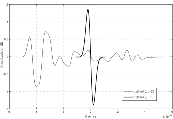
Figure 5: Optimal pulse $p$ for $L\!=\!25$ and basic pulse $q=p$ for $L\!=\!1$ in time-domain in generic units (GU).

In our simulation we choose $T_{q}:=6T_{0}=N_{q}T_{0}$ and $L=25$ as the filter order of the FCC-optimization. Hence, the optimized pulses have a total time duration of $T_{p}=(L-1)T_{0}+T_{q}=30T_{0}=N_{p}T_{0}$.

The Riesz condition (32) has been already verified in [3] for this particular setup. Theorem 2 uses the normalization $T^{\prime}=1$. Translating between different support lengths $T^{\prime}_{p}=K$ is done by setting $t:=t^{\prime}T_{p}/K$. Now the support of $p(t^{\prime})$ is $[-K/2,K/2]$ with fixed $T^{\prime}=1$. To obtain good shift-orthogonality, we have to choose $M>K$. This we control with an integer multiple $m=2$, i.e. $M=mK=2K$. The support length $T_{s}$ of all the LO (ALO) pulses is then given as

$$\begin{split}T_{\tilde{p}^{T,\circ,M}}&=(N-1)T+T_{p}=(2mK)T_{p}/K+N_{p}T_{0}\\ &=T_{p^{T,\circ,M}}=(2m+1)N_{p}T_{0}=150T_{0}.\end{split}$$ (89)

Now the time slot $[-T_{p^{T,\circ,M}}/2,T_{p^{T,\circ,M}}/2]$ exactly contains $N$ mutually orthogonal pulses $\{p^{T,\circ,M}_{m}\}$, i.e. $N$ orthogonal symbols with symbol duration $T_{s}=T_{p^{T,\circ,M}}$ having all the same energy and respecting strictly the FCC mask. This is a $N$-ary orthogonal signal design, which requires high complexity at receiver and transmitter, since we need a filter bank of $N$ different filters.
Our proposal goes one step further. If we only consider one filter, which generates at the output the centered Löwdin orthonormal pulse $p^{T,\circ,M}$, we can use this as a approximated square-root Nyquist pulse with a PPM shift of $T=T_{p}/K$ to enable $N$-ary OPPM transmission by obtaining almost orthogonality.

Advantages of the proposed design are: a low complexity at transmitter and receiver, a combining of ${\mathbf{g}}$ and $\mathbf{b}$ into a single filter operating with clock rate $1/T_{0}$ and $q$ as input if $T=T_{p}/(T_{0}K)\in{\mathbb{N}}$ , a signal processing ”On the fly” and finally a much higher bit rate compared to a binary-PPM. The only precondition for all this, is a perfect synchronisation between transmitter and receiver. In fact, we have to sample equidistantly at rate of $1/T$. The output of the matched filter $h(-t)=p^{T,\circ,M}(t)$ is given by

$$y(t)=\int_{-\infty}^{\infty}r(\tau)p^{T,\circ,M}(\tau-t)d\tau$$ (90)

and recovers the $m$th symbol. The statistic $l_{m}=y(mT)$ is the correlation of the received signal with the symbol $s_{m}$, see Fig. 4. Note that the shifts have support in the window $[-1.5T_{p^{T,\circ,M}},1.5T_{p^{T,\circ,M}}]$, but are almost orthogonal outside the symbol window $[-T_{p^{T,\circ,M}}/2,T_{p^{T,\circ,M}}/2]$ due to the compactness and approximate shift-orthogonal character of the Löwdin pulse $p^{T,\circ,M}$.

In Fig. 6 the centered orthogonal pulses for $T=5T_{0}=5T_{q}/6$ match almost everywhere the original masked Gaussian monocycle, since the translates are almost non-overlapping, hence they are already almost orthogonal. For $T=T_{0}=T_{q}/6$ the overlap results in a distortion of the centered orthogonal pulses, where the ALO pulses have high energy concentration at the boundary (circulant extension of the Gram Matrix).

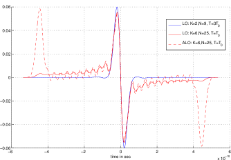
Figure 6: ALO and LO pulses for Gaussian monocycle in time, $L=1$ and $M=2K$.

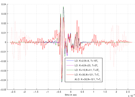
Figure 7: Orthogonal pulses $p^{T,\circ,M}$ with $L=25,M=2K$ and various $T=T_{p}/K$.

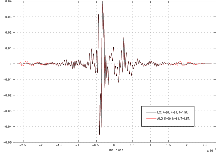
Figure 8: Centered ALO and LO pulse for $T=1.5T_{0}$ with $L=25,M=2K=40$.

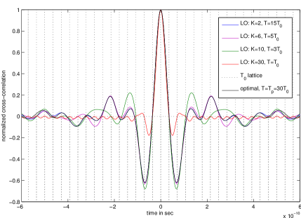
Figure 9: Auto-correlation of pulses for $L=25,T=T_{p}/K$.

In Fig. 7 the pulse shapes in time for the centered Löwdin orthogonal pulses are plotted. The ALO pulses are matching the LO pulses for $T>2T_{0}$ almost perfectly such that we did not plot them, since the resolution of the plot is to small to see any mismatch. Only for the critical shift $T=T_{0}$ a visible distortion is obtained at the boundary. In the next Fig. 8 we plotted therefore the ALO and LO pulse for $T=1.5T_{0}$ to show that the ALO pulses indeed converge very fast to the LO pulse if $T\gg T_{0}$. The reason is that for small time shifts of $p$ the Riesz bounds and so the clustering behaviour of ${{\mathbf{G}}_{M}}$ and ${\mathbf{G}_{M}^{-\frac{1}{2}}}$ decreases. Hence the approximation quality of ${\mathbf{G}_{M}^{-\frac{1}{2}}}$ with ${\mathbf{\tilde{G}}_{M}^{-\frac{1}{2}}}$ decreases, which results in a shape difference.

To study the shift-orthogonal character of the ALO and LO pulses for various $T$, we have plotted the auto-correlations in Fig. 9. As can be seen, the samples $r_{p^{T,\circ,M}}(mT)=\rho_{1m}\approx\delta_{m0}$, i.e. they vanish at almost each sample point except in the origin. The NESP performance for various values of $T$ is shown in Fig. 10. Approaching $T=T_{0}$ cancels the FIR prefilter optimization of ${\mathbf{g}}$, i.e. the spectrum becomes flat. Finally, in Fig. 11 the gain of our orthogonalization strategy can be seen. In both cases, the $N$-ary OOPPM design transmit at an uncoded bit rate of

$$R_{b}(K)=\frac{\log(N)}{T_{s}}=\frac{\log(4K+1)}{150T_{0}}.$$ (91)

Fig. 11 shows the NESP value $\eta$ over the transmit rate $R_{b}$ for $L=25$ and $m=2$. Decreasing $T=T_{p}/K$ results in more overlap, which increases the number of symbols $N$ in $T_{s}$ and hence $R_{b}$, but only slightly decreases $\eta$, see Fig. 10,11.

Summarizing, a triplication of the transmit rate from $0.18$Gbit/s to $0.6$Gbit/s is possible without loosing much signal power ${\mathcal{E}}/T_{s}$ . Let us note the fact that the transmit bit data rate is an uncoded rate and is not an achievable rate. For an analysis of achievable data rates by deriving the mutual information of the system see the work of Ramirez et. al in [16] and Güney et. al in [62]. Obviously, the unshaped Gaussian monocycle then yields the highest transmit rate, since (91) behaves logarithmically in the number $N$ of symbols, as seen in Fig. 11. But this has practically zero SNR when respecting the FCC regulation and results in a high error rate (87),(88). On the other hand, a longer symbol duration, allows in (4) a higher energy ${\mathcal{E}}$ and hence a lower error rate in (11).

Hence, the decreasing of the transmit rate due to the increased symbol duration used for FCC optimal filtering of the masked Gaussian monocycle can be more than compensated by the proposed OOPPM technique.

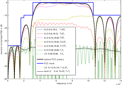
Figure 10: PSD of pulses for $L=25,T=T_{p}/K$.

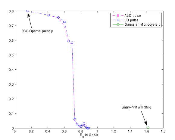
Figure 11: Orthogonalization results of the fixed FCC optimized pulse $p$ for $L=25$ in $T_{s}=150T_{0}$ over various $T$ resulting in various transmit rates $R_{b}$.

7 Conclusion

We have proposed a new pulse design method for UWB-IR which provides high spectral efficiency under FCC constraints and allowing a $N$-ary OPPM transmission with finite transmission and receiving time by keeping almost orthogonality. In fact, the correlation parameters can be keep below the noise level by using small time-shifts $T<T_{p}$. As a result, this provides much higher data rates as compared to BPSK or BPPM. Furthermore, our pulse design provides a N-ary orthogonal PSM transmission by getting a lower bit error rate at the price of a higher complexity.

Simultaneous orthogonalization and spectral frequency shaping is a challenging and hard problem. We believe that for certain shifts being integer multiples of $T_{0}$, a numerical solver might be helpfully to directly solve the combined problem as discusses in Section 5.3.

We highlight the broad application of the OOPPM design, not only being limited to UWB systems but rather applicable to a pulse shaped communication system under a local frequency constraint in general.

Appendix A

Proof of Lemma 1.

Let $a,b\in{\mathbb{R}}$ with $a+b=-1$. Then $S^{a}$ and $S^{b}$, defined by the spectral theorem, are also positive and self-adjoint on ${\mathcal{H}}$. Moreover for each $f$ we have the following unique representation $f=\sum_{k}c_{k}p_{k}$ with ${\mathbf{c}}\in l^{2}({\mathbb{Z}})$ due to the Riesz basis property. For $f=p_{l}$ in (72) we get

$$p_{l} =\sum_{k}\langle S^{-1}p_{l},p_{k}\rangle_{{}_{{\mathcal{H}}}}=\sum_{k}\langle S^{a}p_{l},S^{b}p_{k}\rangle_{{}_{{\mathcal{H}}}}p_{k}$$ (92)

since $$S^{a}p_{l},S^{b}p_{k}\in{\mathcal{H}} {\mathbf{c}}_{l},{\mathbf{d}}_{k} S^{a}p_{l}=\sum_{\alpha}c_{l\alpha}p_{\alpha},S^{b}p_{k}=\sum_{\beta}d_{k\beta}p_{\beta}$$ there exist unique sequences s.t. . Hence we get

$$p_{l} =\sum_{k}\left(\sum_{\alpha}c_{l\alpha}p_{\alpha},\sum_{\beta}d_{k\beta}p_{\beta}\right)p_{k}$$ (93)

$$=\sum_{k}\sum_{\alpha,\beta}c_{l\alpha}\bar{d}_{k\beta}\langle p_{\alpha},p_{\beta}\rangle_{{}_{{\mathcal{H}}}}p_{k}$$ (94)

$$=\sum_{k}\sum_{\alpha,\beta}[{\mathbf{C}}]_{l\alpha}[{\mathbf{G}}]_{\alpha\beta}[{\mathbf{D}}^{*}]_{\beta k}p_{k}=\sum_{k}[{\mathbf{C}}{\mathbf{G}}{\mathbf{D}}^{*}]_{lk}p_{k}$$ (95)

where $c_{l\alpha}$ and $d_{\beta k}$ are the coefficients of the biinfinite matrices ${\mathbf{C}}$ resp. ${\mathbf{D}}$. Since for each $l\in{\mathbb{Z}}$ we have $\sum_{k}\delta_{lk}p_{k}=p_{l}$ and $\{[{\mathbf{C}}{\mathbf{G}}{\mathbf{D}}^{*}]_{lk}\},\{\delta_{lk}\}\in\ell^{2}$, we get $0=\sum_{k}([{\mathbf{C}}{\mathbf{G}}{\mathbf{D}}^{*}]_{lk}-\delta_{lk})p_{k}$ for each $l\in{\mathbb{Z}}$. So by [42, Th.6.1.1(vii)] we can conclude that $[{\mathbf{C}}{\mathbf{G}}{\mathbf{D}}^{*}]_{lk}=\delta_{lk}$ for all $l,k\in{\mathbb{Z}}$ and get

$${\mathbf{C}}{\mathbf{G}}{\mathbf{D}}^{*}={\mathbf{1}}\Leftrightarrow\ {\mathbf{G}}={\mathbf{C}}^{-1}({\mathbf{D}}^{*})^{-1}\Leftrightarrow\ {\mathbf{G}}^{-1}={\mathbf{D}}^{*}{\mathbf{C}}.$$ (96)

Obviously ${\mathbf{D}}$ and ${\mathbf{C}}$ are not an unique decomposition of $S^{-1}$, since $a$ and $b$ are not. If $a=b=-\frac{1}{2}$, we have ${\mathbf{D}}^{*}={\mathbf{C}}^{*}$ and hence ${\mathbf{G}^{-\frac{1}{2}}}={\mathbf{C}}={\mathbf{D}}$. This establishes (73) in an $L^{2}$-sense. ∎

Appendix B

Proof of Theorem 3.

Let us first note that $V(p)$ is a regular SI space since $p$ is a stable generator. This has as consequence that frames are Riesz bases for $V(p)$ [61, Th. 2.2.7 (e)]. So any element $f\in V(p)=p{\ *^{\prime}\,}{\mathbf{c}}$ is uniquely determined by an $\ell^{2}$ sequence ${\mathbf{c}}$. By the Riesz–Fischer Theorem this sequence ${\mathbf{c}}$ defines by its Fourier series a unique $L^{2}([0,1])$-function $\tau=\hat{{\mathbf{c}}}$. Hence, the Fourier transform of any $f\in V(p)$ is represented uniquely by $\tau$ as $\hat{f}=\tau\hat{p}$, see also [37, Th.2.10(d)]. On the other hand $f$ is an orthonormal generator if and only if $\Phi_{f}=1$ a.e.. By using the periodicity of $\tau$ we get

$$\Phi_{f} =\sum_{k}\left|\hat{p}(\cdot-k)\right|^{2}\left|\tau(\cdot-k)\right|^{2}$$ (97)

$$=\left|\tau\right|^{2}\sum_{k}\left|\hat{p}(\cdot-k)\right|^{2}=\left|\tau\right|^{2}\cdot\Phi_{p}=1.$$ (98)

Thus, we have $\left|\tau\right|=1/\sqrt{\Phi_{p}}$ almost everywhere. Let us set $\tilde{\tau}:=1/\sqrt{\Phi_{p}}$ a.e. and a complex periodic phase function $\phi:=e^{i\alpha(\cdot)}:{\mathbb{R}}\to\left\{\left.z\in{\mathbb{C}}\rule[-2.5pt]{0.0pt}{10.0pt}\;\right|\;\left|z\right|=1\right\}$ with $\alpha:{\mathbb{R}}\to[0,2\pi]$ $1$-periodic and measurable. Then any function $\tau\in L^{2}([0,1])$ which satisfy (98) a.e. is given by $\tau=\tilde{\tau}\cdot\phi$ a.e.. The $L^{2}$-distance is then given by

$$\left\|p-f\right\|^{2}_{L^{2}} =\left\|\hat{p}-\hat{f}\right\|^{2}_{L^{2}}=\left\|\hat{p}-\tau\hat{p}\right\|^{2}_{L^{2}}=\left\|p\right\|^{2}_{L^{2}}+\left\|\tau\hat{p}\right\|^{2}_{L^{2}}-\int_{\mathbb{R}}\tau\left|\hat{p}\right|^{2}-\int_{\mathbb{R}}{\overline{\tau}}\left|\hat{p}\right|^{2}$$ (99)

$$=2-\int_{\mathbb{R}}(\tau+{\overline{\tau}})\left|\hat{p}\right|^{2}=2-2\int_{\mathbb{R}}\cos(\alpha)\ \left|\hat{p}\right|^{2}{\Phi_{p}}^{\!-\frac{1}{2}}$$ (100)

$$\geq 2-2\int_{\mathbb{R}}{\left|\hat{p}\right|^{2}}{\Phi_{p}}^{\!-\frac{1}{2}}=2\left(1-\langle p,p^{\circ}\rangle_{{}_{{\mathcal{H}}}}\right).$$ (101)

Since $\left|\hat{p}\right|^{2}$ is positive and $\Phi_{p}$ is bounded and strictly positive a.e. the distance is minimized if and only if $\alpha(\nu)=0$ a.e. in ${\mathbb{R}}$, i.e. if we have equality in (101). Hence $\phi=1$ a.e. and so $\tilde{\tau}=\tau$ a.e., which corresponds hence to the unique orthonormal Löwdin generator $f=p^{\circ}$ with an $L^{2}$-distance to $p$ given in (101). ∎

Remark. Note, that in fact the phase function $\phi$ has no influence on the power spectrum $|\hat{p}^{\circ}_{\phi}|^{2}=\left|\phi\tilde{\tau}\hat{p}\right|^{2}=\left|\tilde{\tau}\hat{p}\right|^{2}=\left|\hat{p}^{\circ}\right|^{2}.$

References

References

- [1] P.-O. Löwdin, On the nonorthogonality problem connected with the use of atomic wave functions in the theory of molecules and crystals, J. Chem. Phys. 18 (1950) 367–370.
- [2] P.-O. Löwdin, On the nonorthogonality problem, Advances in Quantum Chemistry 5 (1970) 185–199.
- [3] P. Walk, P. Jung, Löwdin’s approach for orthogonal pulses for UWB impulse radio, in: IEEE Workshop on Signal Processing Advances in Wireless Communications, 2010.
- [4] P. Walk, P. Jung, J. Timmermann, Löwdin transform on FCC optimized UWB pulses, in: IEEE WCNC, 2010. doi:10.1109/WCNC.2010.5506503.
- [5] FCC, Revision of part 15 of the commission’s rules regarding ultra-wideband transmission systems, ET Docket 98-153 FCC 02-48, First Report and Order, released: April 2002. (February 2002).
- [6] X. Luo, L. Yang, G. B. Giannakis, Designing optimal pulse-shapers for ultra-wideband radios, J. Commun. Netw. 5 (4) (2003) 344–353.
- [7] Z. Tian, T. N. Davidson, X. Luo, X. Wu, G. B. Giannakis, Ultra wideband wireless communication:ultra wideband pulse shaper design, Wiley, 2006. doi:10.1002/0470042397.
- [8] S.-P. Wu, S. Boyd, L. Vandenberghe, Applied and Computational Control, Signals and Circuits: 5. FIR filter design via spectral factorization and convex optimization, Birkhauser, 1999.
- [9] X. Wu, Z. Tian, T. Davidson, G. Giannakis, Optimal waveform design for UWB radios, IEEE Trans. Signal Process. 54 (2006) 2009–2021.
- [10] M. K. Simon, S. M. Hinedi, W. C. Lindsey, Digital communication techniques: signal design and detection, Prentice Hall, 1994.
- [11] J. B. Anderson, Digital transmission engineering, Wiley-IEEE Press, 2005. doi:10.1002/0471733660.
- [12] J. G. Proakis, Digital Communications, McGraw Hill, Singapore, 2001.
- [13] X. Wu, Z. Tian, T. N. Davidson, G. B. Giannakis, Orthogonal waveform design for UWB radios, in: Proceedings of the IEEE Signal Processing Workshop on Advances in Wireless Communications, 2004, pp. 11–14.
- [14] I. Dotlic, R. Kohno, Design of the family of orthogonal and spectrally efficient uwb waveforms, IEEE Journal of Selected Topics in Signal Processing 1 (1) (2007) 21–30. doi:10.1109/JSTSP.2007.897045.
- [15] B. Parr, B. Cho, K. Wallace, Z. Ding, A novel ultra-wideband pulse design algorithm, IEEE Commun. Lett. 7 (5) (2003) 219–222.
- [16] F. Ramirez-Mireles, Performance of UWB N-orthogonal PPM in AWGN and multipath channels, in: IEEE Transactions on Vehicular Technology, 2007, pp. 1272–1285. doi:10.1109/TVT.2007.895488.
- [17] I. Bar-David, G. Kaplan, Information rates of photon-limited overlapping pulse position modulation channels, IEEE Trans. Inf. Theory 30 (1984) 455–463.
- [18] S. Zeisberg, C. Müller, J. Siemes, A. Finger, PPM based UWB system throughput optimisation, in: IST Mobile Communications Summit, 2001.
- [19] I. Daubechies, The wavelet transform, time-frequency localisation and signal analysis, IEEE Trans. Inf. Theory 36 (5) (1990) 961–1005. doi:10.1109/18.57199.
- [20] A. Janssen, T. Strohmer, Characterization and computation of canonical tight windows for gabor frames, J. Fourier. Anal. Appl. 8(1) (2002) 1–28. doi:10.1007/s00041-002-0001-x.
- [21] A. C. Gordillo, R. Kohno, Design of spectrally efficient hermite pulses for psm uwb communications, IEICE Transactions on Fundamentals of Electronics, Communications and Computer Sciences 8 (2008) 2016–2024.
- [22] D. Middleton, An introduction to statistical communication theory, 3rd Edition, International Series in pure and applied physics, IEEE Press, New York, 1996, IEEE Press Reissue.
- [23] R. A. Scholtz, Multiple access with time-hopping impulse modulation, in: IEEE Military Communications Conference, Vol. 2, Boston, MA, 1993, pp. 447–450. doi:10.1109/MILCOM.1993.408628.
- [24] M. Z. Win, R. A. Scholtz, Impulse radio: how it works, IEEE Commun. Lett. 2 (2) (1998) 36–38. doi:10.1109/4234.660796.
- [25] M. Z. Win, Spectral density of random time-hopping spread-spectrum UWB signals with uniform timing jitter, in: IEEE Military Communications Conference, Vol. 2, 1999, pp. 1196–1200. doi:10.1109/MILCOM.1999.821393.
- [26] F. Ramirez-Mireles, R. A. Scholtz, Multiple-access with time hopping and block waveform ppm modulation, 1998.
- [27] Y.-P. Nakache, A. F. Molisch, Spectral shape of UWB signal influence of modulation format, multiple access scheme and pulse shape, in: Proceedings of the IEEE Vehicular Technology Conference, 2003.
- [28] M. Z. Win, Spectral density of random UWB signals, IEEE Commun. Lett. 6 (12) (2002) 526– 528. doi:10.1109/LCOMM.2002.806458.
- [29] S. li Wang, J. Zhou, H. Kikuchi, Performance of overlapped and orthogonal th-bppm uwb systems, in: IEEE Conference on Wireless Communications, Networking and Mobile Computing, 2008.
- [30] S. Villarreal-Reyes, R. Edwards, Spectrum shaping of PPM TH-IR based ultra wideband systems by means of the PPM modulation index and pulse doublets, in: Antennas and Propagation Society International Symposium, 2005 IEEE, 2005.
- [31] Y.-P. Nakache, A. F. Molisch, Spectral shaping of UWB signals for time-hopping impulse radio, Selected Areas in Communications, IEEE Journal on 24 (2006) 738 – 744.
- [32] C. Berger, M. Eisenacher, S. Zhou, F. Jondral, Improving the UWB pulseshaper design using nonconstant upper bounds in semidefinite programming, IEEE Journal of Selected Topics in Signal Processing 1 (3) (2007) 396–404. doi:10.1109/JSTSP.2007.906566.
- [33] Y. Liu, Q. Wan, Designing optimal UWB pulse waveform directly by FIR filter, in: International Conference on Wireless Communications, Networking and Mobile Computing, 2008.
- [34] T. Davidson, Z.-Q. Luo, J. F. Sturm, Linear matrix inequality formulation of spectral mask constraints with applications to FIR filter design, IEEE Trans. Signal Process. 50 (11) (2002) 2702– 2715. doi:10.1109/TSP.2002.804079.
- [35] C. R. Berger, M. Eisenacher, H. Jäkel, F. Jondral, Pulseshaping in UWB systems using semidefinite programming with non-constant upper bounds, in: IEEE Int. Symp. on Personal, Indoor and Mobile Radio Communications, 2006.
- [36] J. F. Sturm, Using SeDuMi 1.02, a MATLAB toolbox for optimization over symmetric cones, Optimization Methods and Software 11 (1) (1999) 625–653. doi:10.1080/10556789908805766.
- [37] C. d. Boor, R. A. DeVore, A. Ron, The structure of finitely generated shift-invariant spaces in , Journal of Functional Analysis 119 (1994) 37–78.
- [38] A. Aldroubi, Q. Sun, Locally finite dimensional shift-invariant spaces in , Proceedings of the American Mathematical Society 130 (9) (2002) 2641–2654.
- [39] A. Aldroubi, M. Unser, Sampling procedures in function spaces and asymptotic equivalence with shannon’s sampling theory, Journal Numerical Functional Analysis and Optimization 15 (1994) 1 – 21.
- [40] R.-Q. Jia, Shift-invariant spaces on the real line, Proc. Amer. Math. Soc. 125 (1997) 785–793.
- [41] J. J. Benedetto, S. Li, The theory of multiresolution analysis frames and applications to filter banks, Applied and Computational Harmonic Analysis 5 (1998) 389–427. doi:10.1006/acha.1997.0237.
- [42] O. Christensen, An introduction to frames and Riesz bases, Birkhauser, 2003.
- [43] Y. Meyer, Ondelettes et fonctions splines., Séminaire Équations aux dérivées partielles 6 (1986) 1–18.
- [44] K. Gröchenig, Foundations of time-frequency analysis, Springer Verlag, 2001.
- [45] R. Landshoff, Quantenmechanische Berechnung des Verlaufes der Gitterenergie des Na-Cl-Gitters in Abhaengigkeit vom Gitterabstand, Zeitschrift für Physik A 102 (3-4) (1936) 201–228. doi:10.1007/BF01336687.
- [46] P. Jung, Weyl–Heisenberg representations in communication theory, Ph.D. thesis, Technical University Berlin (2007).
- [47] A. Aldroubi, Q. Sun, W.-S. Tang, p-frames and shift invariant subspaces of , Journal of Fourier Analysis and Applications 7 (2001) 1–22.
- [48] A. Böttcher, S. M. Grudsky, Spectral properties of banded Toeplitz matrices, Siam, 2005.
- [49] G. Strang, A proposal for toeplitz matrix calculations, Stud. Apply. Math. 74 (1986) 171–176.
- [50] P. J. Davis, Circulant matrices, Wiley, 1979.
- [51] A. J. E. M. Janssen, The Zak transform: A signal transform for sam- pled time-continuous signals, Philips J. Res. 43 (1988) 23–69.
- [52] R. H.-F. Chan, X.-Q. Jin, An Introduction to Iterative Toeplitz Solvers, SIAM, 2007.
- [53] R. M. Gray, Toeplitz and circulant matrices, Foundations and Trends in Communications and Information Theory 2 (2006) 155–239.
- [54] J. Gutierrez-Gutierrez, P. M. Crespo, Asymptotically equivalent sequences of matrices and hermitian block toeplitz matrices with continuous symbols: Applications to mimo systems, IEEE Transactions on Information Theory 54 (12) (2008) 5671–5680. doi:10.1109/TIT.2008.2006401.
- [55] F.-W. Sun, Y. Jiang, J. Baras, On the convergence of the inverses of toeplitz matrices and its applications, IEEE Transactions on Information Theory 49 (1) (2003) 180–190. doi:10.1109/TIT.2002.806157.
- [56] P. Casazza, O. Christensen, N. J. Kalton, Frames of translates, Collect. Math. 52 (2001) 35–54.
- [57] Y. Zhu, J. Zuegel, J. Marciante, H. Wu;, Distributed waveform generator: A new circuit technique for ultra-wideband pulse generation, shaping and modulation, IEEE Journal of Solid-State Circuits 44 (3) (2009) 808 – 823. doi:10.1109/JSSC.2009.2013770.
- [58] H. L. V. Trees, Detection, Estimation, and Modulation Theory, Wiley, 1968.
- [59] I. Jacobs, Comparisson of m-ary modulation systems, Bell Syst. Tech. J 46 (5) (1967) 843–864.
- [60] R.-Q. Jia, C. A. Micchelli, Curves and surfaces, San Diego, 1991, Ch. Using the refinement equations for the construction of Pre-Wavelets II: powers and two.
- [61] A. Ron, Shen, Frames and stable bases for shift-invariant subspaces of , Tech. rep., Wisconsin University Madison (1994).
- [62] N. Güney, H. Delic, F. Alagöz, Achievable information rates of ppm impulse radio for uwb channels and rake reception, IEEE Trans. Commun. 58 (5) (2010) 1524 – 1535.