Viscosity and Diffusion: Crowding and Salt Effects in Protein Solutions

Abstract

We report on a joint experimental-theoretical study of collective diffusion in, and static shear viscosity of solutions of bovine serum albumin (BSA) proteins, focusing on the dependence on protein and salt concentration. Data obtained from dynamic light scattering and rheometric measurements are compared to theoretical calculations based on an analytically treatable spheroid model of BSA with isotropic screened Coulomb plus hard-sphere interactions. The only input to the dynamics calculations is the static structure factor obtained from a consistent theoretical fit to a concentration series of small-angle X-ray scattering (SAXS) data. This fit is based on an integral equation scheme that combines high accuracy with low computational cost. All experimentally probed dynamic and static properties are reproduced theoretically with an at least semi-quantitative accuracy. For lower protein concentration and low salinity, both theory and experiment show a maximum in the reduced viscosity, caused by the electrostatic repulsion of proteins. The validity range of a generalized Stokes-Einstein (GSE) relation connecting viscosity, collective diffusion coefficient, and osmotic compressibility, proposed by Kholodenko and Douglas [PRE, 1995, 51, 1081] is examined. Significant violation of the GSE relation is found, both in experimental data and in theoretical models, in semi-dilute systems at physiological salinity, and under low-salt conditions for arbitrary protein concentrations.

Sec. I Introduction

A quantitative understanding of the dynamics in concentrated solutions of interacting proteins is of importance to the evaluation of cellular functions, and the improvement of drug delivery. Transport properties such as collective and self-diffusion coefficients, and the static and high-frequency shear viscosities, are strongly affected by the aqueous environment Ball2008 , and in particular by crowding effects due to high concentration of macromolecules, coupled both by direct and solvent-mediated, hydrodynamic interactions (HIs) Ellis2001 ; Zimmerman1993 ; Skolnick2010 . The latter type of interaction, which is both long-ranged and of many-body nature, poses a particularly challenging task to a theoretical treatment of diffusion and rheological transport properties.

In the present paper, we report on a combined experimental and theoretical study on collective diffusion, low shear-rate static viscosity, and static and dynamic scattering functions of concentrated solutions of bovine serum albumin (BSA) proteins. The goal of this study is twofold. On the one hand, we explore how far a simple colloidal model in combination with state-of-the-art theoretical schemes can capture the microstructure and dynamics of proteins in solution. On the other hand, we investigate the concentration- and salt-dependence of collective diffusion and the static shear viscosity, and use our results to test the validity range of a generalized Stokes-Einstein (GSE) relation which combines the collective diffusion coefficient with the isothermal osmotic compressibility and the shear viscosity.

BSA is a protein which is readily soluble in water and stable over a wide range of salt and protein concentrations. Its stability and reproducibility make it well-suited as a model system of globular proteins. Proteins constitute identical solute units surpassing any synthetic colloid suspension in terms of monodispersity. In this respect, they are ideally suited to the application of analytical theoretical models used with good success for large colloids. However, the construction of a quantitatively accurate theoretical model for protein solutions is considerably obstructed not only by the potential presence of impurities and oligomers, but also by the complex internal conformation and surface of a protein. The folding state depends on various control parameters such as temperature, protein concentration, pH value, and salinity. The irregular protein surface implies an orientation-dependent protein interaction energy with repulsive and attractive parts, and furthermore complicates the description of hydroynamically influenced transport properties.

In a first step towards calculating dynamic properties of proteins, it is nonetheless possible to use a model of reduced complexity, with system parameters such as the pH-dependent particle charge determined from a consistent fit of theoretical expressions for the scattered intensity to the experimental static scattering functions. We use here a simple colloid model where the BSA interactions are described by the repulsive, electrostatic plus hard-core part of the isotropic Derjaguin-Landau-Verwey-Overbeek (DLVO) potential Verwey_Overbeek1948 . The effect of the non-spherical shape of BSA proteins is accounted for in the static intensity calculations within the so-called translational-orientational decoupling approximation, by describing the proteins as oblate spheroids interacting by a spherically symmetric effective pair potential.

Using this simplifying protein interaction model, the static structure factor, $S(q)$, entering into the static scattered intensity, is calculated as a function of wavenumber $q$, by using our newly developed modified penetrating background corrected rescaled mean spherical approximation (MPB-RMSA). This analytical method has been shown to be in excellent accord with numerically expensive computer simulation results for $S(q)$ Heinen2011 ; Heinen_Erratum_2011 . The system parameters of the protein-interaction model, most notably the effective protein charge, are determined from adjusting the theoretically calculated static intensity, $I(q)$, to the experimental one. The consistent agreement of calculated values and small-angle X-ray scattering (SAXS) data for $I(q)$ in a wide range of concentrations and wavenumbers indicates that left-out attractive interaction contributions are of minor importance at the considered salinities. As an independent additional check, the static light scattering (SLS) data for $S(q)$ at low $q$ are found to be well reproduced by the theoretical fits of the SAXS data.

Without any further adjustment, the analytically calculated static structure factors are used as the only input to our theoretical calculations of the collective diffusion coefficient, $d_{C}$, and the low shear-rate limiting static viscosity $\eta$. To calculate $d_{C}$ and the high-frequency part, $\eta_{\infty}$, of the static viscosity, we use two approximate analytical schemes, namely the pairwise additive hydrodynamic interaction (PA) approximation, and the so-called self-part corrected $\delta\gamma$ method. As shown by two of the present authors Heinen_TheoArticlePreparation , these two methods give results which are in general in good agreement with more elaborate Stokesian Dynamics simulation results for particles with Yukawa-type pair interactions.

The static viscosity,

$$\eta=\eta_{\infty}+\Delta\eta,$$ (1)

consists of a short-time part, $\eta_{\infty}$, determined solely by hydrodynamic interactions (HIs), and a shear-stress relaxation part $\Delta\eta$, with $\Delta\eta>0$. We calculate the latter using mode-coupling theory (MCT), which, like the two employed short-time schemes, requires $S(q)$ as the only input.

Our comparison with the experimental $d_{C}$ measured by dynamic light scattering (DLS), and with $\eta$ obtained from viscometry, is a stringent test for our theoretical results and for the employed isotropic interaction model, since except for the static input, no fit parameters are involved. In particular, no further adjustments of the theoretical predictions have been made on referring to the actually non-spherical shape of BSA proteins. We show that despite the simplicity of our model, most dynamic features are well reproduced by the theoretical results, to an at least semi-quantitative accuracy. In particular, both a low-concentration maximum of the reduced viscosity, and a maximum in $d_{C}$ at a different concentration, are well captured by the theory.

For BSA, also the short-time self-diffusion has been recently found to be reasonably well described by a simple spheroid model Roosen-Runge2011 ; Roosen-Runge2010 . Of course, this does not imply that the complex conformation of a globular protein plays no role. The DLVO model (even with inclusion of van der Waals attraction) is not sufficient to fully explain the rich phase behavior of proteins. For example, it has been shown that surface patchiness has an important effect on the phase diagram Goegelein2008 . Also, binding of multivalent ions to the protein surface can give rise to non mean-field behaviors beyond DLVO, such as charge inversion, re-entrant condensation and liquid-liquid phase separation Zhang2008 ; Zhang2010 ; Zhang2011 .

Generalized Stokes-Einstein (GSE) relations, which approximately relate diffusion to rheological properties in concentrated complex liquids, are an important issue in microrheological studies, since a valid GSE relation allows to infer a rheological property more easily from diffusion measurements. Several GSE relations in colloidal dispersions of electrically neutral (porous and non-porous) spheres, and charged particle suspensions have been explored Banchio1999GSESs ; Bergenholtz1998GSE ; Banchio2008 ; Abade2010GSE . We study here a GSE relation not discussed in this earlier work, which has been proposed by Kholodenko and Douglas Kholodenko1995 . This GSE relation, which we refer to in the following as the KD-GSE relation, has been used in the biophysical and soft matter community Gaigalas1995 ; Cohen1998 ; Boogerd2001 ; Nettesheim2008 . It relates $d_{C}$ to $\eta$, and to the square-root of the isothermal osmotic compressibility.

We present a thorough discussion of the validity range of the KD-GSE relation for BSA solutions, and for generic colloidal fluids of particles with screened Coulomb interactions, for a large range of salinities. Both the short-time and the long-time versions of the KD-GSE relation are considered. At high salinity, where the electrostatic interaction of particles is strongly screened, we find these two relations to become invalid at larger concentrations. At lower salinity, the KD-GSE relations are poorly satisfied even at low concentrations.

The paper is organized as follows. Sec. II includes the experimental details of the sample preparation, and of the SLS, DLS, SAXS, and rheological measurements. In Sec. III, we discuss the employed simplifying model of BSA, and present the essentials of our theoretical methods, allowing for a fast calculation of measured static and dynamic properties. Our experiment data are shown in combination with the theoretical results in Sections IV and V, dealing with static and dynamic properties, respectively. Sec. V includes the examination of the KD-GSE relation. Our conclusions are contained in Sec. VI.

Sec. II Experimental details

Sample preparation

BSA is a globular protein with a linear extension of about $7$ nm. The considered aqueous solutions of BSA with no added salt, and with monovalent added salt such as NaCl, have a pH in between 5.5 and 7. Under these conditions, BSA is stable in solution, folded in its native state, and carrying a negative net charge in the range of roughly $8$ to $20$ elementary charge units (see below for details) peters1985serum ; Bohme2007 . BSA was purchased from Sigma (cat. A3059) as a lyophilized powder, certified globulin- and protease free.

The sample preparation for all experimental techniques started with the dissolution of protein powder in a solvent, and subsequent waiting until the solution was homogenized. The protein mass concentration, $c_{p}$, in the solution volume, $V_{\textrm{H}_{2}\textrm{O}}+m_{p}\cdot\theta$, is given by the BSA weight $m_{p}$ via

$$c_{p}=\frac{m_{p}}{V_{\textrm{H}_{2}\textrm{O}}+m_{p}\cdot\theta}\quad,$$ (2)

with the specific protein volume $\theta=0.74$ ml/g Lee1974 determines the self-volume of proteins upon dissolution.

For small-angle X-ray scattering, deionized and degased water was used as solvent. The samples with concentrations higher than 15 mg/ml were prepared directly, while smaller concentrations were prepared from a stock solution of 18 mg/ml. The samples were filled into a plastic syringe and inserted into the capillary during the measurement.

For the viscosity measurements, the solutions were prepared similarly using as solvent both deionized water, and solutions of NaCl in deionized water. The NaCl molarity is calculated from the total solution volume, including the protein self-volume. All solutions used for the viscosity experiments were further degased by a water-jet air-pump.

For our light scattering experiments, stock solutions of BSA proteins in deionized water were mixed with solutions of NaCl in deionized water according to the required concentration. The NaCl molarity is calculated from the total water volume. Then, every sample was pressed with a plastic syringe through a hydrophilized nylon membrane filter with a pore size of $100$ nm (Whatman Puradisc 13), and transferred into a cylindrical glass scattering cell. The cell was sealed immediately with a plastic cap.

The effect of the difference in NaCl concentrations between light scattering and viscosity samples, arising from the slightly differing sample preparation, is negligibly small.

Static and dynamic light scattering

Multi-angle dynamic light scattering (DLS) was performed at various concentrations of protein and added salt, at a temperature of $T=295\leavevmode\nobreak\ \text{K}$. In particular, the BSA mass concentration, $c_{p}$, was chosen between $0.1$ to $150$ mg/ml, and the concentration of added salt was $0$ (no added salt), $5$, $150$ and $500\leavevmode\nobreak\ \text{mM}$. Note that, even in the zero added-salt case, the analysis of the scattering data discussed in Sec. IV reveals a residual electrolyte concentration of a few mM, scaling roughly linear with $c_{p}$ (see Table 1). This suggests a few possible sources of the residual electrolyte ions. Firstly, a possible source could be the surface-released counterions of charged BSA oligomers, not contained in our monodisperse model. Secondly, a salt contamination of the BSA stock, and thirdly the dissociation of acidic or alkaline surface groups off the BSA proteins cannot be excluded.

Static light scattering (SLS) experiments were performed on the same samples. We used a combined SLS/DLS device from ALV (goniometer: CGS3, correlator: 7004/FAST), located at the Institut Laue Langevin in Grenoble, with a minimum correlation time of $3.125\leavevmode\nobreak\ \text{ns}$ as initial and shortest time. The HeNe laser was operating at wavelength $\lambda_{0}=632.8\leavevmode\nobreak\ \text{nm}$, with an output power of $22\leavevmode\nobreak\ \text{mW}$. The accessible range for the scattering angle (wavenumber) was $30\leavevmode\nobreak\ \text{-}\leavevmode\nobreak\ 150^{\circ}$ (q = $0.007\leavevmode\nobreak\ \text{-}\leavevmode\nobreak\ 0.026\leavevmode\nobreak\ \text{nm}^{-1}$). Moreover, the DLS intensity autocorrelation function decays on a time scale much slower than the interaction time, $\tau_{I}\sim\sigma_{d_{0}}^{2}/(4d_{0})\sim 0.3\leavevmode\nobreak\ \mu\text{s}$, of BSA, where $d_{0}$ is the single protein average translational free-diffusion coefficient, and $\sigma_{d_{0}}$ is an effective hydrodynamic diameter. Hence, DLS probes the long-time collective diffusion of BSA, in the $q\to 0$ limit.

The normalized intensity autocorrelation function obtained from DLS,

$$g_{2}(q,t)=\dfrac{\left<I(\mathbf{q},0)I(\mathbf{q},t)\right>}{{\left<I(\mathbf{q})\right>}^{2}},$$

was fitted according to the Siegert relation, by the double exponential decay function

$$g_{2}(q,t)-1=\left(\sum_{i=1,2}A_{i}\cdot\exp\left[-D_{i}\,q^{2}\,t\right]\right)^{2}\leavevmode\nobreak\ +\textrm{B},$$ (3)

with decay constants $D_{1}$ and $D_{2}$, and amplitudes $A_{1}$ and $A_{2}$. The fit results were essentially the same with and without the background-correction constant B. At all probed angles, the two decay constants are widely separated ($D_{1}\gg D_{2}$). The faster mode, $D_{1}$, is attributed to the (long-time) collective diffusion coefficient, $d_{C}$, of BSA monomers. The appearance of the slower mode characterized by $D_{2}$, can be attributed to the slow motion of the larger impurities and oligomers. After having checked that $D_{1}$ is overall $q$-independent within the experimental resolution, it was averaged with respect to its residual scattering angle fluctuations to gain better statistics. Data on $D_{2}$ are rather noisy in comparison to $D_{1}$, and show no clear dependence on $q$, $c_{p}$, and on the concentration of added salt.

Small-angle X-ray scattering

Aqueous solutions of BSA with mass concentrations between $0.9\leavevmode\nobreak\ \text{mg/ml}$ and $270\leavevmode\nobreak\ \text{mg/ml}$, and without added salt, were measured by small-angle X-ray scattering (SAXS), at the beam line ID02 of the European Synchrotron Radiation Facility (ESRF) in Grenoble, France. The standard configuration at a 2m sample-to-detector distance, and a photon energy of 16051 eV was used. Measurements were repeated several times in the flow mode and with short detection times to ensure the absence of radiation damage. The data from the CCD were processed with the standard routines available at the beam line for radially averaging the data and correcting for transmission. Repeated measurements were summed up, and the solvent scattering was measured independently and subtracted from the data. Additionally, two dilute samples (at $c_{p}=1$ and $2$ mg/ml) with $150\leavevmode\nobreak\ \text{mM}$ of added NaCl were measured for form factor fitting.

Viscosity measurements

The viscosity data were measured at $T=25^{\circ}$ C, for different concentrations of protein and added salt. The first dataset was obtained for solutions without added salt, while the second set describes systems with $150\leavevmode\nobreak\ \text{mM}$ NaCl. All measurements were performed at a shear rate of $60\leavevmode\nobreak\ \text{Hz}\ll 1/\tau_{I}$, using the suspended couette-type viscometer described in Ref. Bano2003 . The important advantage of this instrument is the possibility to collect data without errors caused by the surface shear-viscosity. A test made for $c_{p}\approx 20$ mg/ml and $100$ mg/ml, without salt and for 2M added NaCl, revealed no shear-rate dependence of the viscosity for shear rates between $50$ and $95\leavevmode\nobreak\ \text{Hz}$. The precision of the viscosity measurements is approximately $0.1\%$. In order to minimize systematic errors, every measurement was repeated three times, including separate sample preparations.

The viscometer directly measures the relative shear-viscosity of the solution against pure water (for technical details see Ref. Bano2003 ). For the aqueous BSA solutions without added salt discussed in this work, the relative viscosity was directly measured. For BSA solutions with added salt, this quantity was obtained as the ratio of the following two values: (a) the directly measured relative viscosity of the BSA solution with salt against water divided by (b) the directly measured relative viscosity of the salt solution (without BSA) against water.

Sec. III Theory

Single-particle properties

In the following, we discuss the spheroid model of BSA. We use this model for the form factor fitting, and in determining effective sphere diameters related to different single-particle properties.

At low protein concentration and sufficient amount of added salt, inter-protein correlations are negligible. The scattered intensity, $I(q)$, is then solely determined by the form factor $P$, i.e. $I(q)\propto P(q)$. Crystallographic measurements Carter1994 ; Ferrer2001 ; Leggio2008 have revealed a flat and roughly heart-shaped structure of albumins. The computation of single-particle properties with an account of the highly complex particle shape of biomolecules can be done by numerical simulations only and is beyond the scope of this paper DeLaTorre2010 ; Ferrer2001 . Rather, the aim of the present study is to give an essentially analytic description of the microstructure and the dynamics of interacting BSA proteins with low computational cost. We therefore intentionally choose an extremely simple model for the fit of the protein form factor, by an oblate, solid ellipsoid (spheroid). Clearly, this mapping of the complex protein configuration onto an essential geometric shape is a delicate and broad topic on its own. Considering that the focus of the present work is on collective correlations rather than on single-particle properties, we cannot discuss all details of this subtle matter; we basically follow the approach of Ref. Zhang2007 .

For a homogeneously scattering spheroid with dimensions $a$ and $b$, where $a$ denotes the semi-axis of revolution, the orientationally averaged form factor, $P_{ell}$, is given by Pedersen1997

$$P_{ell}(q)=\int_{0}^{1}d\mu{|f(q,\mu)|}^{2}$$ (4)

with the scattering amplitude $f(q,\mu)=3j_{1}(u)/u$, and $u=q\sqrt{a^{2}\mu^{2}+b^{2}(1-\mu^{2})}$. Here, $j_{1}$ is the spherical Bessel function of the first kind.

The fit of Eq. (4) to our newly recorded, low-concentration SAXS intensities at $c_{p}=1$ and $2$ mg/ml, and for $150$ mM of added NaCl, is shown in Fig. 1 of Sec. IV, along with a discussion of the obtained best fit values $a=1.75$ nm and $b=4.74$ nm.

When protein correlations come into play at higher concentrations or lower salinities, the spheroid model of BSA becomes too complex for an analytic treatment. Therefore, as far as the protein-protein interactions are concerned, we describe the proteins as effective spheres with diameter $\sigma$. Depending on the considered single-particle property, different definitions for $\sigma$ can be given.

Consider first the geometric effective diameter, $\sigma_{geo}=8(ab^{2})^{1/3}=6.80\leavevmode\nobreak\ \text{nm}$, which follows from equating the volume of the effective sphere to that of the spheroid. This effective diameter reflects the volume of the protein and the hydration layer visible to SAXS, but does not include thermo- and hydrodynamic effects of non-sphericity Svergun1998 ; Zhang2011a . Thus, it should be considered as a lower boundary to the effective sphere diameter.

A thermodynamic effective diameter, $\sigma_{B_{2}}=7.40\leavevmode\nobreak\ \text{nm}$, follows from demanding equal second virial coefficients, $B_{2}(T)$, of hard spheroid and effective hard sphere Isihara1950 .

Alternatively, dynamic single-particle properties can be used in defining the effective diameter. For hydrodynamic stick-boundary conditions and $a<b$, the translational free diffusion coefficient of an isolated spheroid reads Jennings1988 ; Ferrer2001 ; Perrin1936

$$d_{0}^{ell}(a,b)=\dfrac{k_{B}TS(a,b)}{12\pi\eta_{0}a},\\$$ (5)

with absolute temperature $T$, Boltzmann’s constant $k_{B}$, solvent shear-viscosity $\eta_{0}$, $S(a,b)=2\leavevmode\nobreak\ \text{atan}\leavevmode\nobreak\ \xi(a,b)/\xi(a,b)$ and $\xi(a,b)=\sqrt{\left|a^{2}-b^{2}\right|}\leavevmode\nobreak\ /a$. Equating $d_{0}^{ell}$ to the diffusion coefficient, $d_{0}=k_{B}T/(3\pi\eta_{0}\sigma_{d_{0}})$, of an effective sphere gives $\sigma_{d_{0}}=7.38\leavevmode\nobreak\ \text{nm}$.

Finally, one can derive another effective diameter from the intrinsic viscosity

$$[\eta]=\lim_{\phi\to 0}\frac{\eta(\phi)-\eta_{0}}{\eta_{0}\phi},$$ (6)

where $\phi$ is the particle volume fraction. For a spheroid with hydrodynamic stick-boundary conditions Jeffery1922 ; Philipse2001 ,

$$[\eta]^{ell}=\dfrac{5}{2}+\frac{32}{15\pi}\left[\dfrac{b}{a}-1\right]-0.628\left[\frac{1-a/b}{1-0.075a/b}\right],$$ (7)

which for $a=b$ reduces to the Einstein result, $[\eta]^{sph}=2.5$, for a solid sphere. Note here that $[\eta]^{ell}>2.5$ for $a\neq b$. Explicitly, $[\eta]^{ell}=3.25$ for the best fit values $a$ and $b$ given in Fig. 1. On demanding equality of the interaction-independent linear terms in the virial expansions of the viscosity,

$$\dfrac{\eta}{\eta_{0}}=1+[\eta]\phi+\mathcal{O}(\phi^{2}),$$

for spheroids and effective spheres, and on using $\phi^{ell}=(4\pi/3)ab^{2}n$ and $\phi^{sph}=(\pi/6){\sigma_{[\eta]}}^{3}n$ for an equal number density $n$, the effective diameter $\sigma_{[\eta]}=7.42\leavevmode\nobreak\ \text{nm}$ is obtained.

Since the aspect ratio, $b/a=2.71$, is rather close to unity, the four obtained effective diameters are quite similar in magnitude. We use $\sigma=\sigma_{B_{2}}=7.40\leavevmode\nobreak\ \text{nm}$ in all our calculations of static and dynamic properties discussed in this paper.

Static scattering intensity and structure factor

Concentrated protein solutions exhibit pronounced inter-particle correlations which are reflected in the static scattering intensity. This applies also to dilute, low-salinity solutions where the proteins show long-ranged electrostatic repulsion.

In order to allow for an analytical theoretical treatment, we assume that the static scattering intensity of interacting BSA proteins can be approximated by

$$I(q)=Ac_{p}P_{ell}(q)S_{m}(q),$$ (8)

where $S_{m}$ is the so-called measurable static structure factor. Here, $A$ is a $q$-independent factor (of dimension $\text{velocity}^{3}$), that should be the same for all intensity measurements corrected for recording time and source intensity.

For calculating $S_{m}(q)$, we use the rotational-translational decoupling approximation Nagele1996 ; Kotlarchyk1983 , where the spheroid shape is accounted for in the scattering amplitudes only, so that

$$S_{m}(q)=\left[\rule[-5.0pt]{0.0pt}{15.00002pt}1-X(q)\right]+X(q)S(q).$$ (9)

Here,

$$X(q)=\dfrac{1}{P_{ell}(q)}{\left[\int\limits_{0}^{1}d\mu f(q,\mu)\right]}^{2},$$ (10)

with $0\leq X(q)\leq 1$ and $X(q\to 0)=1$, and $S$ is the so-called ideal structure factor of ideally monodisperse effective spheres of diameter $\sigma=\sigma_{B_{2}}$ and screened Coulomb repulsion of DLVO type. For the BSA model spheroid used here, $X(q)$ stays close to unity for $q\lesssim 0.5\leavevmode\nobreak\ \text{nm}^{-1}$, decaying for larger $q$ steeply towards its first zero value at $q\approx 1.3\leavevmode\nobreak\ \text{nm}^{-1}$. For $q>1.3\leavevmode\nobreak\ \text{nm}^{-1}$, $X(q)<0.04$. The orientational disorder assumed in the decoupling approximation has the general effect of damping the oscillations in $S_{m}(q)$. While $S_{m}(q)$ is practically equal to one for $q\gtrsim 1.3\leavevmode\nobreak\ \text{nm}^{-1}$, irrespective of the still visible oscillations in $S(q)$, the effect of orientational disorder on $S_{m}(q)$ is weak in the range $q\lesssim 0.5\leavevmode\nobreak\ \text{nm}^{-1}$, where the most distinctive features in $S(q)$ are seen. We further note that $S_{m}(q\to 0)=S(q\to 0)$ for monodisperse systems, a feature which plays an important role in our upcoming discussion of collective diffusion.

The ideal structure factor, $S(q)$, entering into Eq. (9), is calculated using the repulsive part of the DLVO pair-potential Verwey_Overbeek1948 ,

$$\beta u(x)=\left\{\begin{array}[]{ll}\infty\,,&x=r/\sigma<1,\\ \gamma\;\!\dfrac{{e^{-kx}}}{x}\,,&x>1,\end{array}\right.$$ (11)

also referred to as the hard-sphere Yukawa (HSY) potential. The coupling parameter, $\gamma$, and the screening parameter, $k$, are given by

$$\gamma = \frac{L_{B}}{\sigma}\left(\frac{e^{k/2}}{1+k/2}\right)^{2}\!Z^{2},$$ (12a)

$$k^{2} = k^{2}_{c}+k^{2}_{s}=\frac{L_{B}/\sigma}{1-\phi}\;\!\left(24\phi|Z|+8\pi n_{s}\sigma^{3}\right).$$ (12b)

Here, $L_{B}=\beta e^{2}/\epsilon$ is the solvent-characteristic Bjerrum length in Gaussian units, $\beta=1/(k_{B}T)$, $\epsilon$ is the solvent dielectric constant, and $Z$ is the effective protein charge number in units of the proton elementary charge $e$. The factor $1/(1-\phi)$ in $k^{2}$ corrects for the free volume available to the microions Russel1981 ; Denton2000 . We have not included van der Waals (vdW) forces in $u(x)$. However, we have checked that the influence of vdW attractions is small for most of the considered systems.

Eq. (12b) consists of two additive parts. The first part, $k^{2}_{c}\propto|Z|$, is due to protein-surface released counterions, which are assumed to be monovalent. The second part, $k^{2}_{s}$, accounts for the screening due to all other monovalent microions. Owing to the overall charge neutrality, this contribution is proportional to the co-ion concentration $n_{s}$. A lower bound of $n_{s}\geq 10^{-7}$ M in pH-neutral aqueous solutions is due to the self-dissociation of water. Additional contributions to $n_{s}$ can arise from dissolved CO₂, and added salt such as NaCl. For a protein solution, $n_{s}$ can have a (putatively linear) dependence on $c_{p}$ if charged protein oligomers are present, acting as an additional source of surface-released counterions not contained in our model. Moreover, the protein stock solution might contain a residual amount of salt, and the proteins might dissociate acidic or alkaline surface groups during solvation. Note that due to the overall charge neutrality, the total concentration of monovalent counterions is given by $n_{s}+6\phi|Z|/(\pi\sigma^{3})$.

In recent work Heinen2011 ; Heinen_Erratum_2011 , two of the present authors have derived a computationally efficient integral equation scheme for computing $S(q)$ using the screened Coulomb potential in Eq. (11). This so-called modified penetrating background corrected rescaled mean spherical approximation (MPB-RMSA) shares the analytical simplicity of the widely used RMSA Hansen1982 ; Zhang2007 , but is distinctly more accurate. All calculations of $S(q)$ in this paper are based on the MPB-RMSA.

The spheroid-Yukawa (SY) model used in our calculations of $I(q)$ and $S_{m}(q)$ ignores orientational-translational coupling. Therefore, it can be expected to apply only to fluid-phase BSA solutions when $c_{p}$ is sufficiently low, and when the ionic strength is not too large, so that the anisotropic protein shape and pair-interaction parts are not important. At larger $c_{p}$, there is orientational-translational coupling, and the decoupling approximation becomes invalid. We note again that the possible presence of residual protein oligomers and scattering impurities is not accounted for in our one-component model. The virtue of the SY model, however, is its analytical simplicity. The concentration range in which the SY model is applicable to BSA is examined in Sec. IV.

Since we use a spherically symmetric screened Coulomb plus hard-core pair potential for the protein-protein interactions, a short discussion of the neglected anisotropy in the electric double layer around a charged spheroid is in order here.

The mean electrostatic potential, $\Phi(r,\mu)=\sum_{l=0}^{\infty}\Phi_{l}(r)P_{l}(\mu)$, of a spheroid with a corresponding axisymmetric charge distribution immersed in an electrolyte solution includes in general higher-order multipoles with $l>0$. Here, $r$ is the distance of the spheroid center to the field point, $\mu=\cos\vartheta$ is the cosine of the angle relative to the spheroid rotational symmetry axis, and the $P_{l}$’s are Legendre polynomials.

For large $r$, all multipoles decay asymptotically equally fast according to Yoon1991 ; vanRoij2009 ; vanRoij2011 ; Tellez2010 ; Kjellander2003 ; Likos2004

$$\Phi_{l}(r)\sim f_{l}\dfrac{e^{-\kappa r}}{r},$$ (13)

where $\kappa$ denotes the inverse electrostatic screening length, and $f_{l}$ depends on the charge distribution. This implies that, in principle, the pair interaction energy of two spheroids depends on their relative orientation even when $r\gg\kappa^{-1}$. However, the multipolar strengths, $f_{l}$, for a spheroid with $b/a\sim 1$ can be expected to be small for larger $l$. Moreover, since after orientational averaging, $\left<P_{l}(\mu)\right>_{\mu}=0$ for all $l>0$, our neglect of anisotropic pair interaction contributions can be expected to be reasonable, for systems where the particles can essentially rotate freely.

Short-time diffusion

We summarize here the analytical methods used in calculating the (short-time) collective diffusion coefficient $d_{C}$. These methods require $S(q)$ as their only input, with the BSA protein interactions described by the spherical pair potential in Eq. (11).

The colloidal short-time regime covers correlation times $t$ within $\tau_{B}\ll t\ll\tau_{I}$. Here, $\tau_{B}=m_{p}/(3\pi\eta_{0}\sigma)$ is the momentum relaxation time of a globular protein of mass $m_{p}$. Within a short-time span, a protein has diffused a very small fraction of its size only. For BSA in water, $\tau_{B}\sim 1$ ps, and $\tau_{I}\approx 0.3$ $\mu$s. The BSA short-time dynamics is thus not resolved in our DLS experiment determining the measurable dynamic structure factor, $S_{m}(q,t)$, as a function of wavenumber $q$ and correlation time $t$.

Within the translational-orientational decoupling approximation used in the SY model, $S_{m}(q,t)$ is determined by the right-hand-side of Eq. (9) with $S(q)$ replaced by $S(q,t)$. The latter is the ideal dynamic structure factor of ideally monodisperse, charged effective spheres interacting according to Eq. (11).

Owing to the smallness of the proteins compared to the wavelength of visible laser light used in our DLS experiments, one obtains $t\gg\tau_{I}$ and $q\ll q_{m}$. Here, $q_{m}$ is the wavenumber where $S$ attains its principle peak value. Since $X(q\ll q_{m})\approx 1$, it follows that $S_{m}(q\ll q_{m},t)\approx S(q\ll q_{m},t)$, so that the influence of orientational disorder on the measured $S_{m}(q,t)$ via the spheroid form factor is negligible.

As a consequence, DLS determines the long-time collective diffusion coefficient, $d_{C}^{L}$, according to

$$S_{m}(q\ll q_{m},t\gg\tau_{I})\propto\exp\left[-q^{2}d_{C}^{L}t\right].$$ (14)

The coefficient $d_{C}^{L}$, also referred to as the gradient diffusion coefficient, quantifies the long-time decay of long-wavelength, isothermal protein concentration fluctuations. In Eq. (14), additional scattering contributions to $S_{m}(q,t)$, originating from oligomers and large impurities, are neglected. As discussed in relation to Eq. (3), these give rise to an additional, exponentially decaying mode with a mean diffusion constant, $D_{2}$, which is substantially smaller than $d_{C}^{L}$.

While, in principle, $d_{C}^{L}$ needs to be distinguished from its short-time counterpart $d_{C}^{S}$, with $d_{C}^{L}\leq d_{C}^{S}$, it has been shown Nagele1996 ; Szymczak2004 that the relative difference is very small ($\lesssim 5\%$) even in highly concentrated systems. For solutions like the ones considered in this work, where non-pairwise additive HI contributions are small, $d_{C}=d_{C}^{L}$ becomes practically identical to $d_{C}^{S}$. This allows us to use more simple short-time dynamic methods for calculating $d_{C}$.

To this end, we use two complementary analytical methods, namely a self-part corrected version of the so-called $\delta\gamma$ scheme due to Beenakker and Mazur Heinen_TheoArticlePreparation ; heinen2010short ; Beenakker1983 ; Beenakker1984 ; Genz1991 , denoted here as the corrected $\delta\gamma$ scheme for brevity, and a pairwise additive (PA) approximation of the HIs. The latter becomes exact at very low concentrations, but its prediction for $d_{C}^{S}$ worsens when protein volume fractions $\phi\gtrsim 0.05$ are considered (see our discussion of Fig. 3 in Sec. V). On the other hand, the PA predictions for $\eta_{\infty}$, and for the short-time self-diffusion coefficient $d_{S}$ not considered here, are reliable up to substantially larger volume fractions, as has been ascertained in comparison to Stokesian Dynamics computer simulations Banchio2008 ; Heinen_TheoArticlePreparation and experimental data heinen2010short . The PA expression for $d_{C}^{S}$ reads

$$\dfrac{d_{C}^{S}}{d_{0}} = \dfrac{1}{S(q\to 0)}\left\{\dfrac{d_{S}}{d_{0}}-5\phi+12\phi\int_{1}^{\infty}dxx\left[g(x)-1\right]\right.$$ (15)

$$+24\phi\int_{1}^{\infty}dxx^{2}g(x)\tilde{y}_{12}^{a}(x)$$

$$+\left.8\phi\int_{1}^{\infty}dxx^{2}g(x)\left[\tilde{x}_{12}^{a}(x)-\tilde{y}_{12}^{a}(x)\right]\right\},$$

with $d_{S}$ given in PA approximation by

$$\dfrac{d_{S}}{d_{0}}=1+8\phi\int_{1}^{\infty}dxx^{2}g(x)\left[x_{11}^{a}(x)+2y_{11}^{a}(x)-3\right].\\$$ (16)

The two-body mobility functions, $x_{ij}^{a}$ and $y_{ij}^{a}$, can be expanded analytically in powers of $\sigma/r=1/x$. The short-range mobility parts

$$\tilde{x}_{12}^{a}(x) = x_{12}^{a}(x)-(3/4)\,x^{-1}+(1/8)\,x^{-3},$$

$$\tilde{y}_{12}^{a}(x) = y_{12}^{a}(x)-(3/8)\,x^{-1}-(1/16)\,x^{-3},$$

include all terms in the series expansion in $1/x$ with the far-field terms up to the dipolar level subtracted off. For $x>3$, an explicit analytical expansion to $\mathcal{O}(x^{-20})$ is used Schmitz1988 . Since the series expansion in $1/x$ converges slowly at small separations, accurate numerical tables, which account for lubrication at near-contact distances jeff_oni:84 , are employed for $x<3$.

The only input required in Eqs. (15) and (16) is the radial distribution function $g$, related to $S$ by a one-dimensional Fourier transform Hansen_McDonald1986 . The two functions are obtained in our analysis by the analytical MPB-RMSA.

The second short-time method used in the present work for calculating $d_{C}^{S}\approx d_{C}$ and $\eta_{\infty}$, is the self-part corrected $\delta\gamma$ scheme. In this scheme, $d_{C}^{S}$ is obtained from the exact relation Nagele1996

$$\dfrac{d_{C}^{S}}{d_{0}}\lim_{q\to 0}S(q)=\dfrac{d_{S}}{d_{0}}+\lim_{q\to 0}H_{d}(q)$$ (17)

containing the distinct part, $H_{d}(q)$, of the so-called hydrodynamic function $H(q)$. The $\delta\gamma$ scheme of Beenakker and Mazur provides an easy-to-use integral expression for $H_{d}(q)$, including $S(q)$ as the only required input. The explicit form of the $\delta\gamma$-scheme expression for $H_{d}(q)$ is given in Genz1991 ; Banchio2008 and will be thus not repeated here.

Extensive comparisons with Stokesian Dynamics simulations Banchio2008 , and experiments on charged colloids Gapinski2006 ; heinen2010short , and for small $\phi$ also with PA calculations, have shown that the $\delta\gamma$ scheme predictions for $H_{d}(q)$ are quite good for all concentrations up to the freezing transition value, even though the $\delta\gamma$ scheme involves hydrodynamic approximations at any concentration. In particular, it disregards lubrication effects. Lubrication, however, is inconsequential for charge-stabilized particles where near-contact configurations are unlikely.

Different from $H_{d}(q)$, the accuracy of the $\delta\gamma$ scheme is less good for charged particles regarding the self-part, $d_{S}$, of $d_{C}^{S}$ in Eq. (17) Banchio2008 ; heinen2010short . To remedy this deficiency, we use a hybrid method, referred to as the self-part corrected $\delta\gamma$ scheme, in which $d_{S}$ is calculated using the PA expression in Eq. (16). It has been shown both for charged colloids Banchio2008 ; heinen2010short ; Heinen_TheoArticlePreparation and Apoferritin protein solutions Patkowski2005 , that this hybrid method works quite well at fluid state concentrations.

High-frequency viscosity

The high-frequency viscosity, $\eta_{\infty}$, linearly relates the average suspension shear stress to the average rate of strain in a low-amplitude, high-frequency oscillatory shear experiment. While this short-time quantity has been rather routinely determined for micron-sized charge-stabilized colloids Bergenholtz1998_ExpGSE ; Bergenholtz1998GSE , a direct mechanical measurement of $\eta_{\infty}$ for BSA solutions is difficult, since the required frequencies $\omega\gg\tau_{I}^{-1}$ are in the MHz regime. We are interested here in $\eta_{\infty}$ since, according to Eq. (1), it is an important contribution to the static viscosity $\eta$. The latter has been determined experimentally in the present work.

In PA approximation, $\eta_{\infty}$ is given by Batchelor1972 ; Russel1984 ; Banchio2008

$$\frac{\eta_{\infty}}{\eta_{0}}=1+\frac{5}{2}\phi(1+\phi)+60\phi^{2}\int_{1}^{\infty}dxx^{2}g(x)J(x),$$ (18)

where the rapidly decaying shear mobility function $J(x)$, with $J(x)=15/128\leavevmode\nobreak\ x^{-6}+\mathcal{O}(x^{-8})$ for stick boundary conditions, accounts for two-body HI effects. In performing the integral over $g(x)$, the leading-order long-distance contribution is dominating for $x>3$. Accurate, numerical tables, where the lubrication effect for $x\approx 1$ is included, are used for $x<3$ jeff_oni:84 .

The $\delta\gamma$ scheme of Beenakker and Mazur can be also used for calculating $\eta_{\infty}$. Similar to the $\delta\gamma$-scheme expression for $d_{C}^{S}$, the standard (2${}^{\text{nd}}$ order) $\delta\gamma$ scheme result for $\eta_{\infty}$ consists of a microstructure-independent self-part, and a distinct part given in form of an integral over $S(q)$ Beenakker1984 . In recent work, two of the present authors have shown that a self-part corrected version of the original $\delta\gamma$ scheme expression for $\eta_{\infty}$ gives results for charged particles in very good agreement with Stokesian Dynamics simulations Heinen_TheoArticlePreparation . This self-part corrected $\delta\gamma$ scheme for $\eta_{\infty}$ is used in the present work.

Static shear-viscosity

In long-time rheological measurements on protein solutions under steady shear, there is an additional shear-stress relaxation part, $\Delta\eta$, contributing to the static viscosity $\eta=\eta_{\infty}+\Delta\eta$. This contribution is influenced both by HIs and direct interaction forces. It can be calculated approximately within the mode-coupling theory (MCT) of Brownian systems. While a version of MCT for $\Delta\eta$ with far-field HI included has been discussed in earlier work together with an extension to multicomponent systems Bergenholtz1998 , for analytical simplicity we use here the standard one-component expression

$$\Delta\eta^{MCT}=\dfrac{k_{B}T}{60\pi^{2}}\int_{0}^{\infty}dt\int_{0}^{\infty}dq\leavevmode\nobreak\ q^{4}{\left[\dfrac{S(q,t)}{S(q)}\dfrac{d}{dq}\log S(q)\right]}^{2},$$ (19)

which has been obtained, e.g. in Bergenholtz1998 , under the neglect of HIs. In principle, $\Delta\eta^{MCT}$ should be calculated self-consistently by a numerically expensive algorithm in combination with the corresponding MCT memory equation for $S(q,t)$ Banchio1999 . However, the BSA solutions explored here are rather weakly coupled particle systems, with structure factor maxima $S(q_{m})<1.2$. Thus, as we have thoroughly checked in comparison to fully self-consistent MCT calculations, $\Delta\eta^{MCT}$ can be obtained more simply in a first iteration step where $S(q,t)$ in the integral of Eq. (19) is approximated by its short-time form $S(q,t)/S(q)=\exp[-q^{2}d_{0}t/S(q)]$, valid without HI. The difference to the fully self-consistent result for $\Delta\eta^{MCT}$ is at most a few percent, even for the most concentrated systems considered.

Moreover, again due to the only moderately strong interparticle correlations, $\Delta\eta$ augments $\eta_{\infty}$ by at most ten percent. Therefore, the neglect of HI in $\Delta\eta^{MCT}$ can be expected to be rather insignificant for the systems considered since the dominant effect of HI is included already in $\eta_{\infty}$. Theoretical results for $\eta$ shown in this paper are all based on the first iteration solution for $\Delta\eta^{MCT}$, and on $\eta_{\infty}$ calculated using the self-part corrected $\delta\gamma$ or PA schemes. For all explored systems, the difference in $\eta_{\infty}$ between the PA and corrected $\delta\gamma$ scheme is at most two percent.

Sec. IV Static properties: experiment and theory

IV.1 Form factor fit

Fig. 1: BSA form factor fit. Open circles: SAXS intensities at two protein concentrations of $c_{p}=1$ and $2$ $g/l$, for $150$ mM of added NaCl. The SAXS intensities have been divided by $c_{p}$, and by a common, $q$-independent factor $A_{0}$. Red solid line: Angular-averaged spheroid form factor according to Eq. (4), fitted to the SAXS data within $0.3\leavevmode\nobreak\ \text{nm}^{-1}<q<1.15\leavevmode\nobreak\ \text{nm}^{-1}$, as indicated by the blue vertical line segments. The obtained fit values are $a=1.75$ nm and $b=4.74$ nm. Inset: Intensity on a double linear scale.

In Fig. 1, SAXS intensities for BSA solutions of very small protein weight concentrations, $c_{p}=1$ and $2$ mg/ml, and $150$ mM of added NaCl, are shown along with the best-fit spheroid form factor. Note that our form factor fit relies on a simplified shape model, so that some controlled systematic deviations from experimental data are to be expected. To check for a residual effect of interparticle correlations on $I(q)$, $S(q)$ was calculated for the present two systems to first order in $\phi$ using the full DLVO potential, with $|Z|\sim 30$ and a Hamaker constant of $3k_{B}T$ Lenhoff1996 . The so-obtained structure factor deviates only very little from unity with $S(q\to 0)\approx 0.99$. If vdW attraction is ignored, $S(q\to 0)$ is slightly lowered to $0.98$.

Thus, to fit the measured intensity in Fig. 1, we have used Eq. (8) for $I(q)$ with $S_{m}(q)$ set equal to one. Using an automatic weighted least-squares minimizer, the spheroid semi-axes $a$ and $b$ entering into $P_{ell}(q)$ were varied to achieve a best fit intensity for a given prefactor $A$ in Eq. (8). This fitting procedure was iterated for different values for $A$, until optimal agreement with the SAXS intensities within the range $0.3\leavevmode\nobreak\ \text{nm}^{-1}<q<1.15\leavevmode\nobreak\ \text{nm}^{-1}$ was achieved, resulting in $a=1.75$ nm and $b=4.74$ nm. These values for the spheroid semi-axes are in good accord with previously reported values, and in reasonable agreement with the linear dimensions of the reported heart-shape like crystal structure of albumins Carter1994 ; Ferrer2001 ; Leggio2008 ; Zhang2007 . In a related, recent study by part of the present authors Roosen-Runge2011 , similar values $a=1.80\pm 0.05$ nm and $b=4.60\pm 0.15$ nm have been determined, which are in decent agreement with the values obtained here. The optimized value for $A$, denoted by $A_{0}$, has been also used in our SAXS intensity fits for systems without added salt, which will be discussed in the following subsection.

The best-fit form factor, $P_{ell}$, depicted in Fig. 1 deviates from the SAXS intensities outside the fitted $q$-range. For $q\gtrsim 1.15\leavevmode\nobreak\ \text{nm}^{-1}$, corresponding to length scales $2\pi/q\lesssim 6$ nm $\lesssim\sigma$, the complex internal structure of BSA is probed, which is not accounted for in our simplifying SY model. The deviations visible for $q\lesssim 0.3\leavevmode\nobreak\ \text{nm}^{-1}$, corresponding to distances of roughly $20$ nm or larger, are likely due to additional scattering species made up of larger particles such as BSA oligomers or impurities. Since the size-, form-, and charge-distributions of oligomers and impurities are unknown, our choice of the lower $q$-boundary in fitting $I(q)$ is somewhat more ambiguous than the upper boundary. Therefore, we have repeated the intensity fitting for various low-$q$ boundaries, finding that the weighted least squares deviation increases dramatically if the boundary is selected below $0.3\leavevmode\nobreak\ \text{nm}^{-1}$. Moreover, the fit values for $a$ and $b$ remain essentially constant when the lower $q$-boundary is chosen larger than $0.3\leavevmode\nobreak\ \text{nm}^{-1}$.

The fit parameters of a spheroid form factor to SAXS data of proteins in general depend slightly on the measured $q$ range, the prepared protein concentration, solvent and salt conditions, and background subtraction. In the context of the present study, the related changes of the spheroid model parameters are small compared to the experimental error bars and will be discussed in the next section.

IV.2 Concentration series of scattered intensities

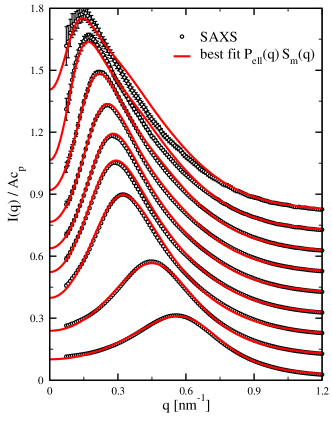
Fig. 2: SAXS intensities from BSA solutions at various $c_{p}$, without added salt, divided by $Ac_{p}$. From top to bottom: $c_{p}=0.9,1.8,4.5,7.2,9,13.5,18,45,$ and $90$ mg/ml. The intensity curves are displaced in steps of $0.1$ along the vertical axis for better visibility. The SAXS-data for the extended range $q\lesssim 4$ $\text{nm}^{-1}$ were taken into account in all fits, but shown here only up to $q=1.2$ $\text{nm}^{-1}$. Red solid lines: best fits according to Eq. (8) with $S(q)$ calculated in MPB-RMSA. The fit parameters are listed in Table 1.

Table 1: Fit parameters $\phi$, $|Z|$, and $A/A_{0}$, for the BSA concentration series without added NaCl, with intensities shown in Fig. 2. The additional parameters $L_{B}=0.711$ nm, $\sigma=\sigma_{B_{2}}=7.40$ nm, $a=1.75$ nm, $b=4.74$ nm are kept fixed, and $A_{0}$ is taken from the form factor fit in Fig. 1. The obtained fit values at $c_{p}=0.9,1.8,45,$ and $90$ mg/ml should be taken with a pinch of salt (see related text). The listed values for $c_{p}$ are according to Eq. (2).

$\mathbf{c_{p}}$ [mg/ml]	$\boldsymbol{\phi}$	$\mathbf{|Z|}$	$\mathbf{n_{s}}$ [$\mathbf{\mu}$M]	$\mathbf{A/A_{0}}$
$0.9$	$5.19\times 10^{-4}$	$34.5$	1216	1.20
$1.8$	$1.34\times 10^{-3}$	$18.8$	608	1.08
$4.5$	$3.72\times 10^{-3}$	$19.1$	1278	0.96
$7.2$	$6.97\times 10^{-3}$	$16.7$	1497	0.97
$9$	$1.04\times 10^{-2}$	$14.6$	1510	1.05
$13.5$	$1.28\times 10^{-2}$	$12.6$	1297	0.81
$18$	$2.06\times 10^{-2}$	$10.8$	1292	0.85
$45$	$8.19\times 10^{-2}$	$9.47$	2375	1.0
$90$	$1.74\times 10^{-1}$	$8.52$	3323	1.0

Fig. 2 includes the SAXS intensities for all explored BSA solutions without added salt that could be fitted using the decoupling approximation expression in Eq. (8), for $S(q)$ calculated in MPB-RMSA using the screened Coulomb potential in Eq. (11). In order to emphasize the shape differences across the dataset, the intensities are divided by their respective fitted amplitudes $A$, and by the protein concentrations $c_{p}$. The most concentrated solution shown here is the one for $c_{p}=90$ mg/ml. Two even more concentrated systems for $c_{p}=180$ and $270$ mg/ml are not depicted in the figure since their intensities could not be fitted reasonably well by the SY model.

In order to fit the experimental intensity data using Eq. (8), some deviations of the prefactor $A$ from the optimized form factor fit value $A_{0}$ have to be allowed for (see Table 1). The fit of each individual intensity curve in Fig. 2 was made as follows: After dividing the SAXS intensity by $A_{0}$ and $c_{p}$, the weighted sum of quadratic deviations between SAXS data points and the intensity according to Eq. (8) was minimized by an automatic three-dimensional weighted least-squares minimizer with respect to the fitting parameters $\left\{|Z|,n_{s},\phi\right\}$. For each concentration, the whole experimental dataset was used, for wavenumbers from $0.07$ to about $4$ $\text{nm}^{-1}$. If the fit was unsatisfactory, the prefactor $A$ was slightly altered, and the optimization with respect to $\left\{|Z|,n_{s},\phi\right\}$ was repeated. This procedure was iterated until convergence in all fit parameters was achieved. For all considered concentrations, $L_{B}=0.711$ nm, $\sigma=\sigma_{B_{2}}=7.40$ nm, $a=1.75$ nm, and $b=4.74$ nm were kept fixed. Table 1 summarizes the obtained best fit parameters.

While the overall intensity fits for the two lowest concentrations, $c_{p}=0.9$ and $1.8$ mg/ml, look quite reasonably good, they contain some peculiarities. A shoulder is present in the fit intensity extending from $q\approx 0.3$ to $0.8$ $\text{nm}^{-1}$, overshooting the experimental data by several standard deviations. Moreover, the prefactor $A$ is substantially larger than $A_{0}$ in both cases, and the fitted effective charge number $|Z|$ assumes a questionably large value of $34.5$ for $c_{p}=0.9$ mg/ml. These peculiarities can be attributed to impurity contributions neglected in Eq. (8). Note also that the maximal intensities in both systems occur at wavenumbers well below the value $0.3$ $\text{nm}^{-1}$, where impurities are found to obstruct also the form factor fit in Fig. 1.

All our attempts to remedy these fitting problems for the two most dilute samples failed. Lacking information about the shape and size distribution, and the interactions of the impurities, we cannot improve on Eq. (8). Restricting the wavenumber interval in the fitting procedure to $q\gtrsim 0.3$ $\text{nm}^{-1}$ leads to no improvement, either. While Eq. (8) is expected to be quite accurate in this restricted $q$-range, the maximum in $I(q)$ is not included. The intensity for $q>0.3$ $\text{nm}^{-1}$ is a monotonically decaying curve, almost completely determined by the form factor. It therefore lacks distinct features coming from particle correlations, rendering the fit with respect to $\left\{|Z|,n_{s},\phi\right\}$ into an overdetermined problem. For all these reasons, our fit parameters in Table 1 for $c_{p}=0.9$ and $1.8$ mg/ml should not be considered as quantitatively accurate.

Except for the two most dilute systems, all other systems with concentrations from $c_{p}=4.5$ to $90$ mg/ml included in Fig. 2 can be excellently fitted by Eq. (8). The obtained effective charges, salt concentrations, and volume fractions all assume reasonable values, showing systematic dependencies on the BSA concentration. Note, however, that for $c_{p}=45$ and $90$ mg/ml, the SY model is pushed to its limit. On assuming a Hamaker constant of $3$ $k_{B}T$ Lenhoff1996 , the repulsive barrier height of the DLVO potential becomes very small, with values of $1.3$ and $0.5$ $k_{B}T$ at $c_{p}=45$ and $90$ mg/ml, respectively. The contact value of $g(x)$ at $x=1$ is just barely zero for the more dilute system, whereas $g(x=1^{+})\approx 0.9$ in the more concentrated system. Obviously, the SY model with purely repulsive, spherically symmetric pair interactions is bound to fail when the particles are allowed to come into hard-core contact. Thus, the system with $c_{p}=45$ mg/ml, and fitted volume fraction $\phi=8.19\%$, is clearly on the borderline of the SY model. Somewhat unexpectedly, and probably fortuitously, the system with $c_{p}=90$ mg/ml can still be fitted with good accuracy. Summarizing, the fit values for the most concentrated systems with $c_{p}=45$ and $90$ mg/ml in Table 1 should be interpreted with caution, since the fit parameters might be significantly distorted by the discussed deficiencies of the SY model. An indication for this could be the obtained fit values for $\phi(c_{p})$, which for the two most concentrated samples clearly overshoot the linear dependence on $c_{p}$ found approximately for the lesser concentrated systems (see Table 1).

In closing our discussion of the static scattered intensities, we note that fit parameters slightly different from the ones in Table 1 are obtained, when in place of the BSA model spheroid axes $(a,b)=(1.75\leavevmode\nobreak\ \text{nm},4.74\leavevmode\nobreak\ \text{nm})$, the values $(a,b)=(1.80\leavevmode\nobreak\ \text{nm},4.60\leavevmode\nobreak\ \text{nm})$ given in Roosen-Runge2011 are used. For instance, at $c_{p}=4.5$ and $18$ mg/ml, the best-fit values for $|Z|$ change to $18.4$ and $10.7$, respectively. Note that, in comparison to Zhang2007 , where the RMSA was employed in fitting $I(q)$, we use here the improved MPB-RMSA integral equation scheme for $S(q)$, resulting in more precise fit-values. Moreover, different from the earlier intensity fitting described in Zhang2007 , the dephasing influence on $I(q)$ originating from the particle asphericity is accounted for approximately in the decoupling approximation used in the present study. The slightly different spheroid semi-axes $(a,b)=(1.80\leavevmode\nobreak\ \text{nm},4.60\leavevmode\nobreak\ \text{nm})$, and the corresponding, slightly changed fit-parameters, do not cause appreciable changes in the dynamical properties. For instance, the collective diffusion coefficient changes by no more than $3\%$, and the changes in the static- and high-frequency viscosities are less than $0.1\%$. Note that the somewhat smaller spheroid causes changes of the fitted volume fraction of about 5% which does not change absolute values but slightly rescales the protein concentration axis for the theoretical predictions.

Sec. V Dynamic properties: experiment and theory

In the following, we compare the DLS data for the collective diffusion coefficient of BSA solutions, and the static shear viscosity measured in our suspended couette-type rheometer, to the results of the dynamic schemes discussed in Sec. III. Moreover, we test the validity of a generalized Stokes-Einstein relation connecting the viscosity to the collective diffusion coefficient and the isothermal osmotic compressibility. We reemphasize here that the employed theoretical schemes use $S(q)$ and $g(r)$ as the only input. With $S(q)$ and $g(r)$ determined from the fits to the SAXS-intensities, all theoretical results for $d_{C}$, $\eta_{\infty}$ and $\eta$ are thus obtained without any additional adjustable parameters.

V.1 Collective diffusion coefficient

Fig. 3 includes our SLS/DLS data for $1/S(q\to 0)$ (upper part) and $d_{C}^{L}=d_{C}$ (lower part), for aqueous BSA solutions in comparison with the theoretical predictions. Systems without added salt, and for concentrations $n_{s}=5$ and $150$ mM of added NaCl, are considered. Additional measurements using $500$ mM of added NaCl (data not shown) agree almost perfectly with the data for $n_{s}=150$ mM, indicating that electrostatic repulsion is fully screened already at $n_{s}=150$ mM. As the input to the dynamics schemes, $S(q)$ and $g(r)$ were generated by the MPB-RMSA, using concentration-interpolated input parameters $\phi(c_{p})$ and $Z(c_{p})$ based on Table 1. For no added salt, $n_{s}(c_{p})$ was interpolated using Table 1, while $n_{s}=5$ and $150$ mM were kept fixed (independent of $c_{p}$) in the corresponding theoretical calculations. The value $d_{0}^{ell}=5.82$ ${\text{\AA}}^{2}/\text{ns}$ of the spheroid translational free diffusion coefficient was used to obtain $d_{C}$ in the experimental units from the dimensionless results for $d_{C}/d_{0}$ obtained by both theoretical schemes.

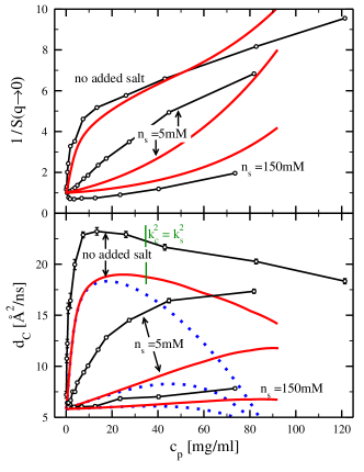
Fig. 3: Top panel: Inverse zero-wavenumber limiting static structure factor of BSA solutions, obtained from SLS (connected black circles) and our MPB-RMSA scheme (red solid lines). Number concentrations, $n_{s}$, of added NaCl as indicated. Bottom panel: Fast mode coefficient, $D_{1}=d_{C}^{L}$, obtained from the discussed double-exponential fit to the DLS data of BSA solutions (connected black circles), and $d_{C}^{S}$ calculated by the self-part corrected $\delta\gamma$ scheme (red solid lines), and the PA approximation (blue dotted curves). All theoretical curves are based on input parameters $\phi(c_{p})$ and $Z(c_{p})$ interpolated from Table 1. In the zero added-salt case, the $n_{s}(c_{p})$ values were also interpolated using Table 1. Theoretical results for added NaCl are obtained using fixed salt concentrations of $n_{s}=5$ and $150$ mM. The input parameters $L_{B}=0.711$ nm, $\sigma=\sigma_{B_{2}}=7.40$ nm, $a=1.75$ nm, $b=4.74$ nm, and $d_{0}=d_{0}^{ell}(a,b)=5.82\leavevmode\nobreak\ \text{\AA}^{2}/\text{ns}$ are kept fixed throughout. For the zero added-salt case, the green vertical line segment at $c_{p}\approx 34$ mg/ml marks the protein mass-concentration where the surface-released counterion contribution to $k^{2}$ in Eq. (12b) is equal to the coion contribution.

For no added salt, the experimental $d_{C}(c_{p})$ assumes a maximum at $c_{p}\approx 10-20$ mg/ml. This maximum is qualitatively reproduced by both theoretical schemes (corrected $\delta\gamma$ and PA), but its location is predicted to occur at somewhat larger concentrations $c_{p}\approx 20-30$ mg/ml. For BSA concentrations larger than the concentration at the maximum value for $d_{C}$, the PA-predicted $d_{C}(c_{p})$ reduces strongly, eventually reaching unphysical negative values for $c_{p}\gtrsim 110$ mg/ml. This illustrates the expected failure of the PA scheme at higher concentrations, indicating that three-body contributions to HI, totally left out in the PA, but not in the $\delta\gamma$ scheme, come into play for $c_{p}\gtrsim 30$ mg/ml. Up to the concentration value at the maximum of $d_{C}$, both schemes agree very well, with residual differences not visible for $c_{p}\lesssim 20$ mg/ml on the scale of Fig. 3. Despite its residual small inaccuracies, the self-part corrected $\delta\gamma$ expansion will therefore be used in the following calculations of $d_{C}$.

The physical origin of the non-monotonous concentration dependence $d_{C}(c_{p})$ at low concentrations of salt can be understood on the basis of Eq. (15), rewritten using $d_{C}\approx d_{C}^{S}$ as

$$\dfrac{d_{C}}{d_{0}}=\lim_{q\to 0}\dfrac{H(q)}{S(q)},$$ (20)

with $H(q)=d_{s}/d_{0}+H_{d}(q)$. The ratio in Eq. (20) consists of two competing factors. The factor $1/S(q\to 0)$, inversely proportional to the isothermal osmotic compressibility of ideally monodisperse particles, increases monotonically as a function of the BSA concentration. Owing to the larger coupling constant $\gamma$ in Eq. (12a), a much steeper initial increase of $1/S(q\to 0)$ is observed for weakly screened systems than for systems with added salt (c.f. the top panel of Fig. 3). As $c_{p}$ is further increased, the amount of surface-released counterions increases correspondingly, leading to an enhanced electrostatic screening. As a consequence, the rate of change of $1/S(q\to 0)$ with $c_{p}$ reduces significantly at a colloid concentration roughly set by the criterion, $k_{c}^{2}(c_{p})=k_{s}^{2}$, of equal surface released counterion and salt-co-ion contributions to the screening parameter in Eq. (12b).

The nominator in Eq. (20) is the reduced sedimentation velocity, $H(q\to 0)$, which is known from theory and experiment heinen2010short to decrease monotonically, for not too large concentrations and low salinity according to $1-a_{sed}\leavevmode\nobreak\ \phi^{1/3}$, with $a_{sed}=1.6\leavevmode\nobreak\ -\leavevmode\nobreak\ 1.8$ in the case of highly charged particles, and as $1-6.546\leavevmode\nobreak\ \phi+21.918\leavevmode\nobreak\ \phi^{2}+\mathcal{O}(\phi^{3})$ for neutral hard spheres Cichocki2002 . For strongly correlated particles, the competition between decreasing compressibility and decreasing sedimentation coefficient with increasing $c_{p}$ leads thus to a maximum in $d_{C}(c_{p})$, at a concentration roughly determined from $k_{c}^{2}(c_{p})=k_{s}^{2}$.

The DLS-measured values for $d_{C}$ are not quantitatively reproduced by the self-part corrected $\delta\gamma$ scheme. Both in the zero added-salt case, and for $n_{s}=150$ mM, $d_{C}$ is underestimated by the corrected $\delta\gamma$ scheme prediction by about $25\%$. The difference might be simply due to the complex-shaped BSA proteins having a translational free diffusion coefficient larger than the value $d_{0}^{ell}=5.82$ ${\text{\AA}}^{2}/\text{ns}$ used in the SY model. In fact, an extrapolation of the experimental data for $d_{C}$ to zero concentration leads to a larger value for $d_{0}$ in the range of $6-7$ ${\text{\AA}}^{2}/\text{ns}$, which can completely explain the differences in $d_{C}$ between experiment and theory. However, this low-concentration extrapolation should not be over-interpreted as being conclusive, since the experimental data are rather noisy for low concentrations.

While the agreement between the theoretical and the experimental $d_{C}$’s is overall rather satisfying for very low and very high salt content, strong differences are found for the intermediate added NaCl concentration of $5$ mM. This is not surprising, however, since already the zero added-salt experiments led to fit values for $n_{s}$ of $1$ to $3$ mM. Therefore, $n_{s}$ is most probably a function of $c_{p}$ also in the $5$ mM added NaCl case, instead of being constant as assumed in the calculations. Moreover, there is no obvious reason to expect that the relation $Z(c_{p})$, interpolated from Table 1, remains valid at arbitrary added salt concentrations. Additional future SAXS measurements at $5$ mM added NaCl are necessary to determine, for this case, the precise dependence of $n_{s}$ and $Z$ on $c_{p}$.

V.2 Static viscosity

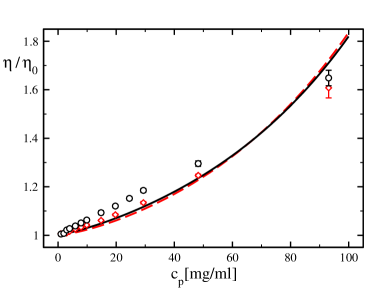
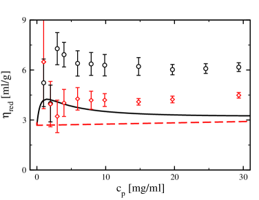
Fig. 4: Static relative (top panel) and reduced (bottom panel) viscosity for $T=25^{\circ}$ C as function of $c_{p}$. Theoretical curves are based on input parameters $\phi(c_{p})$ and $Z(c_{p})$, concentration-interpolated using Table 1. Symbols: experimental data without added salt (black circles) and with $n_{s}=150$ mM (red diamonds). Lines: theoretical results without added salt (black solid line, $n_{s}(c_{p})$ interpolated using Table 1) and with a fixed salt concentration of $n_{s}=150$ mM (red dashed curve). Note the different $c_{p}$-ranges in the two panels of the figure.

The rheometric results for $\eta$ without added salt, and with $150$ mM of added NaCl, are plotted in Fig. 4 as a function of $c_{p}$, and compared to the theoretical predictions. Apart from pronounced differences at lower concentrations, discussed in detail further down, the experimental data agree overall decently well with the theoretical predictions. Due to the rather weak microstructural ordering of the BSA proteins, characterized by structure factor peak heights less than $1.2$ even for the most concentrated samples, the shear-stress relaxation term $\Delta\eta$ contributes only little to $\eta$, with a maximum relative contribution of about $10\%$ near $c_{p}=100$ mg/ml. The dominant contribution to $\eta$ is given by $\eta_{\infty}$, which is predicted to good accuracy both by the PA scheme and the corrected $\delta\gamma$ scheme, with practically equal results. The PA scheme is applicable to the whole experimentally probed concentration range of $c_{p}\lesssim 100$ mg/ml, since three-body and higher order HI contributions affect $\eta_{\infty}$ to a lesser extent than $d_{C}$ (c.f. here Fig. 3, showing the failure of the PA prediction for $d_{C}$ already for $c_{p}\lesssim 50$ $g/l$).

The addition of larger amounts of salt lowers the values for $\eta$, as can be noticed from the two experimental data sets depicted in Fig. 4. The reason for this is the enhanced electrostatic screening, causing $\Delta\eta$ to decrease with increasing salinity in going from strongly structured, charged spheres to basically neutral hard spheres. In contrast, $\eta_{\infty}$ is known from theory and experiment Banchio2008 to increase upon the addition of salt, due to the enlarged influence of near-field HIs when the particles are allowed to get closer to each other in electrostatically screened systems. Thus, $\eta_{\infty}$ and $\Delta\eta$ have opposite trends in their dependencies on the concentration of added salt. These competing trends are the reason for the weak crossover in the two theoretical curves for $\eta$, noticed in the top panel of Fig. 4 at $c_{p}\approx 67$ mg/ml. For particle concentrations larger than this $c_{p}$ value, the increase of $\eta_{\infty}$ overcompensates the decrease in $\Delta\eta$ when, in place of the zero added-salt system, a system with $n_{s}=150$ mM is considered. That such a weak crossover is not observed in the experiment data in Fig. 4, points to an underestimation of the crossover concentration by our simplifying theories for $\eta$, possibly due to the neglect of HIs in the $\Delta\eta$ calculation.

A remarkable feature is noticed from the bottom panel of Fig. 4, where we plot the so-called reduced viscosity,

$$\eta_{red}(c_{p})=\dfrac{\eta(c_{p})-\eta_{0}}{\eta_{0}c_{p}},$$ (21)

as a function of $c_{p}$. The function $c_{p}\eta_{red}/\phi$ reduces to the intrinsic viscosity, $[\eta]$ at very low volume fractions where $\eta\to\eta_{0}+[\eta]\phi$. Features of dilute systems are more clearly revealed in $\eta_{red}$ than in $\eta$.

Both experimental data sets in the bottom panel of Fig. 4 show a local maximum of $\eta_{red}$ at low $c_{p}$ values, which for the zero added-salt system (black open circles) is visible as a weak non-monotonicity near $c_{p}\approx 3$ mg/ml. For the system with $150$ mM added NaCl (red open diamonds), the experimental maximum is represented essentially by a single data point at $c_{p}=1$ mg/ml, where $\eta_{red}\approx 6.5$ ml/g, whereas the remaining data points describe a nearly constant plateau value of $4.5$ ml/g. This plateau value is in good overall agreement with reported values for $\eta_{red}$ at low $c_{p}$, in the range of $3.8$ to $4.9$ ml/g Tanford1956 ; Kupke01081972 ; Placidi1998 ; curvale2008intrinsic .

Regarding the large experiment error bars at very low $c_{p}$, from the figure, we can not attribute physical significance to the single-point maximum in the $n_{s}=150$ mM system. A more refined data resolution in a future experimental study is clearly needed here. Even the maximum in $\eta_{red}$ for the zero added-salt case might be disputable on basis of the experimental data alone. However, the existence of such a maximum in $\eta_{red}$ draws its credibility from the comparison to the theoretical results, showing a maximum in $\eta_{red}(c_{p})$ at a slightly lower value of $c_{p}$. A similar non-monotonic behavior of $\eta_{red}(c_{p})$, with a pronounced peak at low $c_{p}$, has been measured also in polyelectrolyte systems Forster1995 ; Forster1996 ; Eisenberg1977 , in low-salinity suspensions of charged silica spheres Okubo1987 , and in microgels Philipse2002 . The effect has been described theoretically by scaling arguments Rabin1987 , by the Rice-Kirkwood equation Kirkwood1959 for the shear viscosity in combination with a screened Coulomb potential Nishida2004 , and for rod-like particles using a MCT scheme similar to ours Yethiraj2004 . In these earlier treatments, HI has been disregarded altogether. In our approach, HI is included in the for the present systems dominating $\eta_{\infty}$ part of $\eta$.

To rule out that the non-monotonicity of the theoretical $\eta_{red}(c_{p})$ is caused by BSA-specific dependencies of $|Z|$ and $n_{s}$ on $c_{p}$, (c.f. Table 1), we have investigated additionally a model system for fixed $|Z|=20$ and $n_{s}=1$ mM, where we find again a maximum in $\eta_{red}(c_{p})$. Thus, the maximum in $\eta_{red}(c_{p})$ is a generic effect in weakly screened HSY fluids. It is entirely due to the shear-stress relaxation term $\Delta\eta$, for $(\eta_{\infty}-\eta_{0})/(\eta_{0}\phi)$ increases monotonically in $c_{p}$ at arbitrary salt concentration. Since the HIs are neglected in our MCT treatment of the shear-stress relaxation part $\Delta\eta$, we conclude that the local maximum in $\eta_{red}$ is basically a non-hydrodynamic effect, arising from electrostatic repulsion. We point out that the discussed physical mechanism underlying the non-monotonic behavior of $\eta_{red}(c_{p})$ is different from the one causing the maximum in $d_{C}$ as a function of $c_{p}$. The latter maximum originates from a competition between electrostatic repulsion and hydrodynamic slowing in crowded systems. It is therefore not surprising that the maxima in $\eta_{red}$ and $d_{C}$ are located at considerably different protein concentrations. Whereas the maximum of $d_{C}$ occurs at $c_{p}\approx 30$ mg/ml (c.f. Fig. 3), the maximum in $\eta_{red}$ is observed at $c_{p}\lesssim 5$ mg/ml.

The theoretical values for $\eta_{red}$ in Fig. 4 underestimate the experimental data by a factor of about $1/2$. In the low-concentration regime, the theoretical result for $\eta_{red}c_{p}/\phi$ approaches $[\eta]=2.5$, owing to the underlying effective sphere model. The intrinsic viscosity of BSA modeled as a spheroid is $[\eta]^{ell}=3.25$, which is larger than the value for a sphere by a factor of $1.3$ only. Therefore, this can not be the only cause for the observed deviation. However, the actual intrinsic viscosity of a heart-like shaped BSA protein is neither equal to that of a spheroid nor to that of an effective sphere. We recall here our discussion of Fig. 3, where we argued that $d_{0}$ for a BSA protein might well be about $25\%$ larger than the free diffusion coefficient, $d_{0}^{ell}$, of the model spheroid. We can similarly argue that the observed differences between the experimental and theoretical $\eta_{red}$ may be largely due to a value for the intrinsic viscosity of BSA of about $4-5$, which is $20-50\%$ larger than ${[\eta]}^{ell}$, and about twice as large as the $[\eta]$ value of spheres. This could explain the observed difference.

Finally, we note here that electrokinetic contributions to $\eta$, $d_{S}$ and $d_{C}$, originating from the non-instantaneous response of the microion-clouds around each protein, are not included in our treatment. Microion electrokinetics has the effect of lowering somewhat the values of $d_{S}$ and $d_{C}$ Retailleau1999 ; Patkowski2005 , while enlarging the viscosity $\eta$ Ohshima2007 ; Sherwood2007 . These effects can be expected to be stronger when $\kappa^{-1}$ is approximately equal to the particle size. Furthermore, electrokinetic effects are expected to be less significant at higher protein concentrations McPhie2007 ; McPhie2008 .

V.3 Relation between viscosity and collective diffusion

Kholodenko and Douglas Kholodenko1995 have proposed the approximate generalized Stokes-Einstein (GSE) relation

$$\dfrac{d_{C}(\phi)\eta(\phi)}{d_{0}\eta_{0}}\sqrt{S(q\to 0,\phi)}\approx 1,$$ (22)

between collective diffusion coefficient, (static) viscosity and the square-root of the isothermal osmotic compressibility coefficient $S(q\to 0,\phi)$. If this relation were exactly valid, the dimensionless function on the left-hand-side (lhs) of Eq. (22) would be a constant equal to one. The (approximate) validity of a GSE relation would be very useful from an experimental viewpoint, since it allows to infer viscoelastic properties such as $\eta_{\infty}$ and $\eta$ from a dynamic scattering experiment where diffusion coefficients are determined. This is of particular relevance when the amount of protein available is too small for a mechanical rheometer measurement. Since we have experimental data sets for $\eta$, $d_{C}$, and $S(q\to 0)$ for BSA solutions with low and high salt content at our disposal, together with theoretical tools to calculate these properties, we are in the position to scrutinize the accuracy of the KD-GSE relation. We can do this not only for the special case of BSA solutions, but with our theoretical methods more generally for arbitrary spherical colloidal particles interacting by the HSY potential in Eq. (11).

In their discussion of the GSE relation in Eq. (22), based on mode-coupling theory like arguments, Kholodenko and Douglas have considered explicitly a dilute suspension of colloidal hard spheres to first order in $\phi$ only, where $\eta_{\infty}$ and $\eta$ are identical, since $\Delta\eta=\mathcal{O}(\phi^{2})$. For high concentrations, we test now the validity of both the long-time and short-time versions of the KD-GSE relation, on recalling that different from $\eta_{\infty}$ and $\eta$, $d_{C}^{S}$ and $d_{C}^{L}$ are practically equal even at high concentrations.

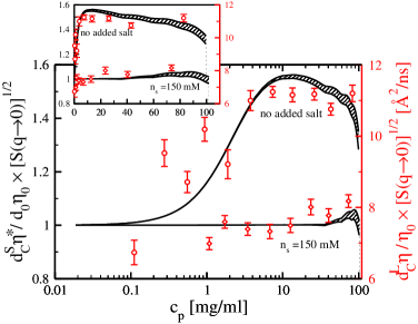
Fig. 5: Test of the long-time and short-time KD-GSE relations in Eq. (22), with $\eta^{*}=\eta$ and $\eta^{*}=\eta_{\infty}$, respectively. Results for BSA solutions without added salt (upper datasets), and with $150$ mM of added NaCl (lower datasets) are shown. Red symbols: combination of $d_{C}^{L}$ from DLS, $\eta/\eta_{0}$ from suspended couette rheometry, and $S(q\to 0)$ from SLS. Black lines: Theoretical results, combining $d_{C}^{S}\approx d_{C}^{L}$ and $\eta_{\infty}$ calculated from the self-part corrected $\delta\gamma$ scheme with $S(q\to 0)$ from the MPB-RMSA scheme. For the long-time GSE version, $\eta=\eta_{\infty}+\Delta\eta$, with $\Delta\eta$ from MCT is used. Lower boundaries of the theoretical curves correspond to the short-time GSE, upper boundaries to the long-time version. The theoretical curves are based on $S(q)$-input with $\phi(c_{p})$ and $Z(c_{p})$ concentration-interpolated using Table 1. For zero added salt, $n_{s}(c_{p})$ was also interpolated on basis of Table 1. The parameters $L_{B}=0.711$ nm and $\sigma=\sigma_{B_{2}}=7.40$ nm are kept fixed.

In Ref. Kholodenko1995 , it was argued that for uncharged hard spheres (HS) the KD-GSE relation is valid to linear order in $\phi$. We can check this statement analytically using numerically precise 2${}^{\text{nd}}$ order virial expansion results for $d_{C}^{HS}={(d_{C}^{S})^{HS}}$, $\eta_{\infty}^{HS}$, $\eta^{HS}$ Cichocki2002 ; Cichocki2003 ; Cichocki1994 , and with $S^{HS}(q\to 0,\phi)$ calculated from the precise Carnahan-Starling equation of state. In this way, we obtain

$$\dfrac{d_{C}^{HS}\eta_{\infty}^{HS}}{d_{0}\eta_{0}}\sqrt{S^{HS}(q\to 0)} = 1-0.046\phi+1.3713\phi^{2}+\mathcal{O}(\phi^{3}),$$

$$\dfrac{d_{C}^{HS}\eta^{HS}}{d_{0}\eta_{0}}\sqrt{S^{HS}(q\to 0)} = 1-0.046\phi+2.282\phi^{2}+\mathcal{O}(\phi^{3}).$$

The short- and long-time versions of the KD-GSE relation for hard spheres are identical to linear order in $\phi$, with a coefficient, $-0.046$, which is not precisely vanishing but close to zero. However, to quadratic order in $\phi$ already, where particle correlations come into play and $\eta_{\infty}$ needs to be distinguished from $\eta$, both GSE variants have distinctly non-zero virial coefficients. Since precise values for the higher-order virial coefficients are not known to date, a test of Eq. (22) for larger $\phi$ can be made only using simulation and experimental data for $d_{C}(\phi)$, $\eta_{\infty}(\phi)$ and $\eta(\phi)$. This test has been performed in Heinen_TheoArticlePreparation , where it is shown that both variants of the KD-GSE relation are approximately valid for hard spheres for $\phi\lesssim 0.1$ only.

Since neutral hard spheres are a special case of the HSY model, attained for $\gamma=0$ or $k\to\infty$, as a matter of principle the validity of the KD-GSE relation for HSY systems is disproved already at this point. However, it still remains to be investigated in which concentration range the two KD-GSE relations are significantly violated when, instead of neutral hard spheres, weakly screened, charged HSY-like particles such as charged proteins are considered. Note here that a virial expansion cannot be reasonably applied to charged particles at lower salinity, since the pair structure functions and thermodynamic properties in these systems depend on $\phi$, $\gamma$ and $k$ in a non-analytical way.

In Fig. 5, we plot the lhs function in Eq. (22), both in its short- and long-time form, as a function of $c_{p}$. Both BSA solutions without added salt, and solutions with $n_{s}=150$ mM are considered. Apart from a constant factor, which is related to the actual value of $d_{0}$ in BSA solutions discussed earlier, the theoretical curves compare reasonably well to the experimental data. There are only small differences in the short-time and long-time GSE curves in the case of BSA solutions.

With the hard-sphere-like behavior of the particles practically reached for $n_{s}=150$ mM, in the added-salt system the two KD-GSE variants apply for concentrations up to $c_{p}\approx 50$ mg/ml, corresponding to $\phi\approx 0.1$. For more concentrated systems, the lhs function in Eq. (22) increases initially, going trough a shallow maximum near $c_{p}\approx 90$ mg/ml. For zero added salt, violation of the KD-GSE relations is observed theoretically at all non-zero concentrations, and can be noticed in our experiment already for $c_{p}\lesssim 1$ mg/ml.

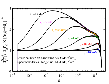
Fig. 6: Test of the short- and long-time versions of the KD-GSE relation in Eq. (22) for volume fractions from very dilute values to $\phi=30\%$, and various salt concentrations as indicated. The collective diffusion coefficient, $d_{C}^{S}/d_{0}\approx d_{C}^{L}/d_{0}$, and high-frequency limiting viscosity, $\eta_{\infty}/\eta_{0}$, are obtained from the self-part corrected $\delta\gamma$ scheme. The static viscosity, $\eta=\eta_{\infty}+\Delta\eta$, is calculated using MCT for $\Delta\eta$. Values for $S(q\to 0)$ are obtained from the MPB-RMSA method. Input parameters $L_{B}=0.711$ nm, $\sigma=7.40$ nm, and $|Z|=10$ are kept constant.

In our discussion of the KD-GSE relation, we proceed now by characterizing the crossover behavior in going from the low-salt to the high-salt regime. To this end, in Fig. 6, we plot the lhs of Eq. (22) as a function of $\phi$ for various salt contents, using the parameters $L_{B}=0.711$ nm, $\sigma=7.40$ nm, and $|Z|=10$. These parameters are typical of aqueous solutions of small globular proteins such as BSA, Lysozyme Goegelein2008 and Apoferritin Patkowski2005 . The charge number $Z$ is kept constant here for simplicity. Theoretical results are plotted as a function of $\phi$ instead of $c_{p}$. In lowering the salt content in Fig. 6 stepwise by factors of $0.1$, starting from a maximal value of $n_{s}=100$ mM, we find that the maximal (positive) deviation from one of the lhs function in Eq. (22) increases roughly logarithmically. For low salt content, $n_{s}\lesssim 1$ mM, the physical origin of the maxima in Fig. 6 is understood from comparing the theoretical results for $d_{C}$ and $\eta$ in Figs.  3 and 4, respectively: The maximal violation of the KD-GSE relations occurs roughly at a volume fraction where $d_{C}(\phi)$ attains its maximum, i.e. for $\phi$ determined approximately from $k^{2}_{c}(\phi)=k^{2}_{s}$. Recalling that $k^{2}_{c}\propto\phi$ and $k^{2}_{s}\propto n_{s}$, this explains why the $\phi$-location of the maxima in Fig. 6 shows a power-law dependence on $n_{s}$ for $n_{s}\lesssim 1$ mM. For larger $n_{s}$, a crossover to hard-sphere-like behavior occurs, where the KD-GSE relations apply for $\phi\lesssim 0.1$.

Sec. VI Conclusions

We have investigated static and dynamic properties of aqueous BSA solutions in an integrated conceptual framework, combining SLS/DLS, SAXS, and rheometric measurements with analytical colloid theory. Solutions with physiological concentrations of added NaCl have been studied, as well as low-salt solutions showing distinct features in the concentration-dependence of the collective diffusion coefficient and the (reduced) viscosity. In our analytical theoretical approach, we have used a simple spheroid-Yukawa model of BSA with isotropic, repulsive pair interactions to calculate the static scattered intensity using the efficient MPB-RMSA method in combination with the orientational-translational decoupling approximation. The form factor fit has been kept intentionally simple, without expecting extreme accuracy. The resulting $S(q)$ have been used without any further fitting, in calculating $d_{C}$, $\eta_{\infty}$, and $\eta$ on basis of our well-tested theoretical methods. We have used the spheroid-Yukawa model for $I(q)$, and the related effective sphere-Yukawa model for the dynamic properties as minimal models without including additional protein-specific features, to clearly reveal the pros and cons of the model. This should help to point out more clearly the significance of left-out protein specific features.

The measured static and dynamic properties of BSA are captured reasonably well in our simplifying SY model, with at least semi-quantitative accuracy, for mass concentrations up to $c_{p}\approx 100$ mg/ml. In the range $2$ mg/ml $\lesssim c_{p}\lesssim 50$ mg/ml, reliable values for the effective protein charge number, and the residual electrolyte concentration, have been obtained from the fits to the SAXS intensities. The SAXS fits are considerably obstructed for $c_{p}\lesssim 2$ mg/ml by the presence of scattering impurities, and by the breakdown of the decoupling approximation for $c_{p}\gtrsim 50$ mg/ml.

A well-developed maximum in the concentration dependence of the collective diffusion coefficient of BSA was found at low salinity. This behavior is seen also in charge-stabilized colloidal suspensions. It is caused by the competition between electrostatic repulsion and hydrodynamic slowing down in crowded systems. Moreover, a non-monotonic concentration dependence of the reduced viscosity of low-salinity BSA solutions was predicted theoretically, and to some extent also seen experimentally. We have explained the local maximum in $\eta_{red}(c_{p})$ as a basically non-hydrodynamic effect caused by electric repulsion. A non-monotonic concentration-dependence of $\eta_{red}$, with a pronounced peak at low concentration, is observed also in polyelectrolyte solutions. Thus, the low-$c_{p}$ peak in $\eta_{red}$ is a generic feature of charge-stabilized dispersions at low salinity.

An essentially concentration-independent underestimation of the experimental $d_{C}$ and $\eta_{red}$ by about $25\%$ and $50\%$, respectively, is made in the theoretical predictions. Possible reasons for this are impurity effects, and an underestimation of the corresponding single-particle coefficients $d_{0}$ and $[\eta]$ through our disregarding of the complex protein shape and hydration shell morphology.

We have analyzed the validity of a GSE relation by Kholodenko and Douglas Kholodenko1995 , which connects the collective diffusion coefficient to the shear viscosity and to the isothermal osmotic compressibility. Despite its appealing simplicity, the KD-GSE relation fails to capture the essential richness of macromolecular collective diffusion. It applies to decent accuracy to electrostatically screened solutions at high salinity, for volume fractions up to about $0.1$. However, it is violated for more crowded high-salt solutions, and for basically all volume fractions under low-salt conditions.

Possible extensions of the present work, which allow to maintain analytical simplicity to some extent, are the inclusion of short-range attractive interactions for suspensions of larger salt content using, e.g. a two-Yukawa pair potential Chen2005 ; Kim2011 , and the inclusion of surface patchiness Goegelein2008 . For the static viscosity of more strongly concentrated protein solutions than considered in the present work, the shear stress relaxation contribution, $\Delta\eta$, can become large in comparison to $\eta_{\infty}$. In calculating $\Delta\eta$, one needs then to account for HI contributions which tend to further enlarge its value. Such an inclusion of HI effects into $\Delta\eta$ can be accomplished on basis of an extended MCT scheme discussed in Refs. Bergenholtz1998 ; Banchio1999 . These extensions will be the subject of a future study.

- (1) P. Ball. Chem. Rev., 108:74–108, 2008.
- (2) R. J. Ellis. Curr. Opin. Struct. Biol., 11:500, 2001.
- (3) S. B. Zimmerman and A. P. Minton. Annu. Rev. Biophys. Biomolec. Struct., 22:27–65, 1993.
- (4) T. Ando and J. Skolnick. Proc. Natl. Acad. Sci. U. S. A., 107:18457–18462, 2010.
- (5) E. J. W. Verwey and J. T. G. Overbeek. Theory of the Stability of Lyophobic Colloids. Elsevier, New York, 1948.
- (6) M. Heinen, P. Holmqvist, A. J. Banchio, and G. Nägele. J. Chem. Phys., 134:044532, 2011.
- (7) M. Heinen, P. Holmqvist, A. J. Banchio, and G. Nägele. J. Chem. Phys., 134:129901, 2011.
- (8) M. Heinen, A. J. Banchio, and G. Nägele. Article in preparation.
- (9) F. Roosen-Runge, M. Hennig, F. Zhang, R. M. J. Jacobs, M. Sztucki, H. Schober, T. Seydel, and F. Schreiber. Protein self-diffusion in crowded solutions. PNAS, 2011.
- (10) F. Roosen-Runge, M. Hennig, T. Seydel, F. Zhang, M. W. A. Skoda, S. Zorn, R. M. J. Jacobs, M. Maccarini, P. Fouquet, and F. Schreiber. BBA-Proteins Proteom, 1804:68 – 75, 2010.
- (11) C. Gögelein, G. Nägele, R. Tuinier, T. Gibaud, A. Stradner, and P. Schurtenberger. J. Chem. Phys., 129:085102, 2008.
- (12) F. Zhang, M. W. A. Skoda, R. M. J. Jacobs, S. Zorn, R. A. Martin, C. M. Martin, G. F. Clark, S. Weggler, A. Hildebrandt, O. Kohlbacher, and F. Schreiber. Phys. Rev. Lett., 101:148101, 2008.
- (13) F. Zhang, S. Weggler, M. J. Ziller, L. Ianeselli, B. S. Heck, A. Hildebrandt, O. Kohlbacher, M. W. A. Skoda, R. M. J. Jacobs, and F. Schreiber. Proteins, 78:3450–3457, 2010.
- (14) F. Zhang, R. Roth, M. Wolf, F. Roosen-Runge, M. W. A. Skoda, R. M. J. Jacobs, M. Sztucki, and F. Schreiber. Article in preparation.
- (15) A. J. Banchio, G. Nägele, and J. Bergenholtz. J. Chem. Phys., 111:8721–8740, 1999.
- (16) J. Bergenholtz, F. M. Horn, W. Richtering, N. Willenbacher, and N. J. Wagner. Phys. Rev. E, 58:R4088–R4091, 1998.
- (17) A. J. Banchio and G. Nägele. J. Chem. Phys., 128:104903, 2008.
- (18) G. C. Abade, B. Cichocki, M. L. Ekiel-Jezewska, G. Nägele, and E. Wajnryb. J. Phys.-Condens. Matter, 22:322101, 2010.
- (19) A. L. Kholodenko and J. F. Douglas. Phys. Rev. E, 51:1081–1090, 1995.
- (20) A. K. Gaigalas, V. Reipa, J. B. Hubbard, J. Edwards, and J. Douglas. Chem. Eng. Sci., 50:1107–1114, 1995.
- (21) D. E. Cohen, G. M. Thurston, R. A. Chamberlin, G. B. Benedek, and M. C. Carey. Biochemistry, 37:14798–14814, 1998.
- (22) P. Boogerd, B. Scarlett, and R. Brouwer. Irrig. Drain., 50:109–128, 2001.
- (23) F. Nettesheim, M. W. Liberatore, T. K. Hodgdon, N. J. Wagner, E. W. Kaler, and M. Vethamuthu. Langmuir, 24:7718–7726, 2008.
- (24) T. Peters. Adv.Protein Chem., 37:161–245, 1985.
- (25) U. Böhme and U. Scheler. Chem. Phys. Lett., 435:342–345, 2007.
- (26) J. Lee and S. Timasheff. Biochemistry, 13:257 – 265, 1974.
- (27) M. Bano, I. Strharsky, and I. Hrmo. Rev. Sci. Instrum., 74:4788–4793, 2003.
- (28) D. C. Carter and J. X. Ho. Adv. Protein Chem., 45:153–203, 1994.
- (29) M. L. Ferrer, R. Duchowicz, B. Carrasco, J. Garcia de la Torre, and A. U. Acuna. Biophys. J., 80:2422–2430, 2001.
- (30) C. Leggio, L. Galantini, and N. V. Pavel. Phys. Chem. Chem. Phys., 10:6741–6750, 2008.
- (31) J. Garcia de la Torre, A. Ortega, D. Amoros, R. Rodriguez Schmidt, and J. G. Hernandez Cifre. Macromol. Biosci., 10:721–730, 2010.
- (32) F. Zhang, M. W. A. Skoda, R. M. J. Jacobs, R. A. Martin, C. M. Martin, and F. Schreiber. J. Phys. Chem. B, 111:251–259, 2007.
- (33) J. S. Pedersen. Adv. Colloid Interface Sci., 70:171–210, 1997.
- (34) D. I. Svergun, S. Richard, M. H. J. Koch, Z. Sayers, S. Kuprin, and G. Zaccai. PNAS, 95:2267–2272, 1998.
- (35) F. Zhang, F. Roosen-Runge, M. W. A. Skoda, R. M. J. Jacobs, M. Wolf, P. Callow, H. Frielinghaus, V. Pipich, S. Prévost, and F. Schreiber. Article in preparation.
- (36) A. Isihara. J. Chem. Phys., 18:1446–1449, 1950.
- (37) B. R. Jennings and K. Parslow. Proc. R. Soc. London Ser. A-Math. Phys. Eng. Sci., 419:137–149, 1988.
- (38) F. Perrin. J. Phys. Radium, 7:1–11, 1936.
- (39) G. B. Jeffery. Proc. R. soc. Lond. Ser. A-Contain. Pap. Math. Phys. Character, 102:161–179, 1922.
- (40) F. M. van der Kooij, E. S. Boek, and A. P. Philipse. J. Colloid Interface Sci., 235:344–349, 2001.
- (41) G. Nägele. Phys. Rep., 272:216–372, 1996.
- (42) M. Kotlarchyk and S.-H. Chen. J. Chem. Phys., 79:2461–2469, 1983.
- (43) W. B. Russel and D. W. Benzing. J. Colloid Interface Sci., 83:163–177, 1981.
- (44) A. R. Denton. Phys. Rev. E, 62:3855–3864, 2000.
- (45) J.-P. Hansen and J. B. Hayter. Mol. Phys., 46:651–656, 1982.
- (46) B. J. Yoon. J. Colloid Interface Sci., 142:575–581, 1991.
- (47) E. Eggen and R. van Roij. Phys. Rev. E, 80:041402, 2009.
- (48) N. Boon and R. van Roij. J. Chem. Phys., 134:054706, 2011.
- (49) C. Alvarez and G. Tellez. J. Chem. Phys., 133:144908, 2010.
- (50) R. Ramirez and R. Kjellander. J. Chem. Phys., 119:11380–11395, 2003.
- (51) N. Hoffmann, C. N. Likos, and J.-P. Hansen. Mol. Phys., 102:857–867, 2004.
- (52) E. Wajnryb, P. Szymczak, and B. Cichocki. Physica A, 335:339–358, 2004.
- (53) M. Heinen, P. Holmqvist, A. J. Banchio, and G. Nägele. J. Appl. Crystallogr., 43:970–980, 2010.
- (54) C. W. J. Beenakker and P. Mazur. Physica A, 120:388–410, 1983.
- (55) C. W. J. Beenakker. Physica A, 128:48–81, 1984.
- (56) U. Genz and R. Klein. Physica A, 171:26–42, 1991.
- (57) R. B. Jones and R. Schmitz. Physica A, 149:373–394, 1988.
- (58) D. J. Jeffrey and Y. Onishi. J. Fluid Mech., 139:261–290, 1984.
- (59) J.-P. Hansen and I. R. McDonald. Theory of Simple Liquids. Academic Press, London, 2 edition, 1986.
- (60) A. J. Banchio, J. Gapinski, A. Patkowski, W. Häussler, A. Fluerasu, S. Sacanna, P. Holmqvist, G. Meier, M. P. Lettinga, and G. Nägele. Phys. Rev. Lett., 96:138303, 2006.
- (61) J. Gapinski, A. Wilk, A. Patkowski, W. Häussler, A. J. Banchio, R. Pecora, and G. Nägele. J. Chem. Phys., 123:054708, 2005.
- (62) J. Bergenholtz, N. Willenbacher, N. J. Wagner, B. Morrison, D. van den Ende, and J. Mellema. J. Colloid Interface Sci., 202:430–440, 1998.
- (63) G. K. Batchelor and J. T. Green. J. Fluid Mech., 56:401–427, 1972.
- (64) W. B. Russel. J. Chem. Soc., Faraday Trans., 80:31–41, 1984.
- (65) G. Nägele and J. Bergenholtz. J. Chem. Phys., 108:9893–9904, 1998.
- (66) A. J. Banchio, J. Bergenholtz, and G. Nägele. Phys. Rev. Lett., 82:1792–1795, 1999.
- (67) C. M. Roth, B. L. Neal, and A. M. Lenhoff. Biophys. J., 70:977–987, 1996.
- (68) B. Cichocki, M. L. Ekiel-Jezewska, P. Szymczak, and E. Wajnryb. J. Chem. Phys., 117:1231–1241, 2002.
- (69) C. Tanford and J. G. Buzzell. J. Phys. Chem., 60:225–231, 1956.
- (70) D. W. Kupke, M. G. Hodgins, and J. W. Beams. Proc. Natl. Acad. Sci. U. S. A., 69:2258, 1972.
- (71) M. Placidi and S. Cannistraro. Europhys. Lett., 43:476–481, 1998.
- (72) R. Curvale, M. Masuelli, and A. P. Padilla. Int. J. Biol. Macromol., 42:133–137, 2008.
- (73) S. Förster and M. Schmidt. In Physical properties of polymers, volume 120 of Adv. in Poly. Sci., pages 51–133. Springer, Berlin, 1995.
- (74) M. Antonietti, A. Briel, and S. Förster. J. Chem. Phys., 105:7795–7807, 1996.
- (75) H. Eisenberg. Biophys. Chem., 7:3–13, 1977.
- (76) T. Okubo. J. Chem. Phys., 87:6733–6739, 1987.
- (77) Y. Dziechciarek, J. J. G. van Soest, and A. P. Philipse. J. Colloid Interface Sci., 246:48–59, 2002.
- (78) Y. Rabin. Phys. Rev. A, 35:3579–3581, 1987.
- (79) S. A. Rice and J. G. Kirkwood. J. Chem. Phys., 31:901–908, 1959.
- (80) K. Nishida, K. Kiriyama, T. Kanaya, K. Kaji, and T. Okubo. J. Polym. Sci. Pt. B-Polym. Phys., 42:1068–1074, 2004.
- (81) K. Miyazaki, B. Bagchi, and A. Yethiraj. J. Chem. Phys., 121:8120–8127, 2004.
- (82) P. Retailleau, M. Riès-Kautt, A. Ducruix, L. Belloni, S. J. Candau, and J. P. Munch. Europhys. Lett., 46:154–159, 1999.
- (83) H. Ohshima. Langmuir, 23:12061–12066, 2007.
- (84) J. D. Sherwood. J. Phys. Chem. B, 111:3370–3378, 2007.
- (85) M. G. McPhie and G. Nägele. J. Chem. Phys., 127:034906, 2007.
- (86) A. J. Banchio, M. G. McPhie, and G. Nägele. J. Phys.-Condes. Matter, 20:404213, 2008.
- (87) B. Cichocki, M. L. Ekiel-Jezewska, and E. Wajnryb. J. Chem. Phys., 119:606–619, 2003.
- (88) B. Cichocki and B. U. Felderhof. J. Chem. Phys., 101:7850–7855, 1994.
- (89) Y Liu, W.-R. Chen, and S.-H. Chen. J. Chem. Phys., 122:044507, 2005.
- (90) J. M. Kim, R. Castaneda-Priego, Y. Liu, and N. J. Wagner. J. Chem. Phys., 134:064904, 2011.