Solution of the quantum harmonic oscillator plus a delta-function potential at the origin: The oddness of its even-parity solutions

Abstract

We derive the energy levels associated with the even-parity wave functions of the harmonic oscillator with an additional delta-function potential at the origin. Our results bring to the attention of students a non-trivial and analytical example of a modification of the usual harmonic oscillator potential, with emphasis on the modification of the boundary conditions at the origin. This problem calls the attention of the students to an inaccurate statement in quantum mechanics textbooks often found in the context of solution of the harmonic oscillator problem.

1 Introduction

Every single book on quantum mechanics gives the solution of the harmonic oscillator problem. The reasons for that are, at least, two: (i) it is a simple problem, amenable to different methods of solution, such as the Frobenius method for solving differential equations [1, 2], and the algebraic method leading to the introduction of creation and annihilation operators [3]. This problem has therefore a natural pedagogical value; (ii) the system itself has immense applications in different fields of physics and chemistry [4, 5] and it will appear time and time again in the scientific life of a physicist.

Another problem often found in quantum mechanics textbooks is the calculation of the bound state (negative energy) of the potential $V(x)=\alpha\delta(x)$, with $\alpha<0$. The latter example is instructive for the student because it cracks down the miss-conception that the continuity of the wave function and its first derivative at an interface is the only possible boundary condition in quantum problems. In fact, for this potential, the first derivative of the wave function is discontinuous at $x=0$. To see the origin of this result, let us write the Schrödinger equation as

$$-\frac{\hbar^{2}}{2m}\frac{d^{2}\psi(x)}{dx^{2}}+\alpha\delta(x)\psi(x)=E\psi(x)\,.$$ (1)

Integrating Eq. (1) in an infinitesimal region around $x=0$ we get [3]

$$\lim_{\epsilon\rightarrow 0}\left.\frac{d\psi(x)}{dx}\right|_{-\epsilon}^{+\epsilon}-\frac{2m\alpha}{\hbar^{2}}\psi(0)=0\Leftrightarrow\psi^{\prime}_{>}(0)-\psi^{\prime}_{<}(0)=\frac{2m\alpha}{\hbar^{2}}\psi(0),$$ (2)

where $\psi_{\gtrless}(x)$ are the wave functions in each side of the delta potential and we have used Newton’s notation for derivatives where the primes over functions denote the order of the derivative of that function. It is clear from Eq. (2) that the first derivative of the wave function is discontinuous. An explicitly calculation gives the eigenstate of the system in the form

$$\psi(x)=\sqrt{\kappa}\,e^{-\kappa|x|},$$ (3)

which has a kink at the origin as well as a characteristic length scale given by $\kappa=m\alpha/\hbar^{2}$. The eigenvalue associated with the wave function (3) is $E=-\hbar^{2}\kappa^{2}/(2m)$. When $E>0$, the system has only scattering states for both positive and negative values of $\alpha$. We now superimpose a harmonic potential potential on the already present delta-function potential. Due to the confining harmonic potential, the new system only has bound states, no mater the sign of $\alpha$ and $E$. Thus, the problem we want to address is the calculation of the eigenstates and eigenvalues of the potential

$$V(x)=\frac{m}{2}\omega^{2}x^{2}+\alpha\delta(x)\,.$$ (4)

As we will see, this problem has both “trivial” and non-trivial solutions. Furthermore, it allows a little excursion into the world of special functions. Indeed, special functions play a prominent role in theoretical physics, to a point that the famous Handbook of Mathematical Functions, by Milton Abramowitz and Irene Stegun [6], would be one of the three texts (together with the Bible and Shakespeare complete works) Michal Berry would take with him to a desert island [7]. In a time where symbolic computational software is becoming more and more the source of mathematical data, we hope with this problem to show that everything we need can be found the good old text of Milton Abramowitz and Irene Stegun [6].

In addition, this problem will call the attention of students to an inaccurate statement in quantum mechanics textbooks often found in the context of the solution of the harmonic oscillator problem. Our approach is pedagogical, in the sense that illuminates the role of boundary conditions imposed on the even-parity wave functions by the $\delta-$function potential. (We note that after the submission of this article, the work by Busch et al. [8] was brought to our attention; see note added at the end of article.)

2 Solution of the harmonic oscillator with a delta-function

The Hamiltonian of the system is

$$H=-\frac{\hbar^{2}}{2m}\frac{d^{2}}{dx^{2}}+\frac{m}{2}\omega^{2}x^{2}+\alpha\delta(x)\,.$$ (5)

Following tradition, we introduce dimensionless variables using the intrinsic length scale of the problem $a_{0}^{2}=\hbar/(m\omega)$. Making the substitution $y=x/a_{0}$ in Eq. (5) we can write the Schrödinger equation as

$$\frac{d^{2}\psi(y)}{dy^{2}}+(2\epsilon-y^{2})\psi(y)+2g\delta(y)\psi(y)=0\,,$$ (6)

where $\epsilon=ma_{0}^{2}E/\hbar^{2}$ and $g=\alpha a_{0}m/\hbar^{2}$. With $g=0$, Eq. (6) is recognized as the Weber-Hermite differential equation [1]. In quantum mechanics textbooks, the solution of Eq. (6) with $g=0$ proceeds by making the substitution

$$\psi(y)=e^{-y^{2}/2}w(y)\,.$$ (7)

At same time, it is a common practice to write $2\epsilon=2\nu+1$, where $\nu$ is a real number. This allow us to transform Eq. (6) into

$$w^{\prime\prime}-2yw^{\prime}+2\nu w-2g\delta(y)w=0\,,$$ (8)

which is Hermite’s differential equation when $g=0$; a further substitution, $z=y^{2}$, transforms the Eq.(8) into the Kummer’s equation,

$$zw^{\prime\prime}+(b-z)w^{\prime}-a\nu w=0~{}~{}~{}~{}~{}~{}\mathrm{with}~{}a=-{\textstyle\frac{\nu}{2}}~{}\mathrm{and}~{}b={\textstyle\frac{1}{2}}\,,$$ (9)

which, obviously, has two linearly independent solutions: the confluent hypergeometric functions $M(a,b,z)$ and $U(a,b,z)$; these functions also known as Kummer’s functions (the latter solution is sometimes referred as Tricomi’s function) . Thus, the general solution of Eq. (9) is

$$w(z)=A_{\nu}\,M(-{\textstyle\frac{\nu}{2}},{\textstyle\frac{1}{2}},z)+B_{\nu}\,U(-{\textstyle\frac{\nu}{2}},{\textstyle\frac{1}{2}},z),$$ (10)

where $A_{\nu}$ and $B_{\nu}$ are arbitrary complex constants and $\nu$ is an arbitrary real number. The $U(-{\textstyle\frac{\nu}{2}},{\textstyle\frac{1}{2}},z)$ function can also be written in terms the functions $M(a,b,z)$ as [9, a]

$$U\left({\textstyle\frac{\nu}{2}},{\textstyle\frac{1}{2}},z\right)=\pi\left\{\frac{M\left(-{\textstyle\frac{\nu}{2}},{\textstyle\frac{1}{2}},z\right)}{\Gamma\left({\textstyle\frac{1}{2}}\right)\Gamma\left({\textstyle\frac{1}{2}}-{\textstyle\frac{\nu}{2}}\right)}-\sqrt{z}\frac{M\left({\textstyle\frac{1}{2}}-{\textstyle\frac{\nu}{2}},\frac{3}{2},z\right)}{\Gamma\left(\frac{3}{2}\right)\Gamma\left(-{\textstyle\frac{\nu}{2}}\right)}\right\}.$$ (11)

It is important to note that Eq. (11) is not a linear combination of two $M(a,b,z)$ functions. Using Eq. (11), it is possible to show that if $\nu$ is either zero or a positive integer number (denoted by $n$), the solution in Eq. (10) can put in the following form ($z>0$):

$$w(z)\propto\left\{\begin{array}[]{ll}M(-{\textstyle\frac{n}{2}},{\textstyle\frac{1}{2}},z)&\mathrm{for}~{}n~{}\mathrm{even}\\ \sqrt{z}\,M({\textstyle\frac{1}{2}}-{\textstyle\frac{n}{2}},{\textstyle\frac{3}{2}},z)&\mathrm{for}~{}n~{}\mathrm{odd},\\ \end{array}\right.$$

or more compactly [9, b,c], it can be written as $w(z)\propto H_{n}(\sqrt{z})$, with $H_{n}(z)$ the Hermite polynomial of order $n$; further more the product $w(z)e^{-|z|}$ converges for all $z$. Then, the full wave function has the usual form

$$\psi_{n}(y)\propto e^{-y^{2}/2}H_{n}(y),$$

with the corresponding eigenvalues being $\epsilon=n+{\textstyle\frac{1}{2}}$. What we have detailed above condenses the typical solution of the quantum harmonic oscillator using special functions.

We now move to the solution of the quantum harmonic oscillator with a $\delta$-function potential at the origin. To that end, we have to review few properties of the $M(a,b,z)$ functions. For non-integer values of $a$ and $b$, the $M(a,b,z)$ function is a convergent series for all finite given $z$ [9, a], but diverges for $z\rightarrow+\infty$ as [9, d]

$$M(a,b,z)=\frac{\Gamma(b)}{\Gamma(a)}e^{z}z^{a-b}[1+O(|z|^{-1})].$$ (12)

In terms of the original variable $y^{2}$, the function (12) diverges as $e^{y^{2}}$, which implies that $\psi(y)$ also diverges at infinity as $e^{y^{2}/2}$. Thus, $\psi(y)$ is not, in general, an acceptable wave function.

We noted at the introduction to this article that it is many times referred (erroneously) in most standard textbooks on quantum mechanics that the only mathematical solutions of the harmonic oscillator differential equation that does not blow up when $y\rightarrow+\infty$ are those having $\nu$ either zero or a positive integer.

On the contrary however, the function $U(-{\textstyle\frac{\nu}{2}},{\textstyle\frac{1}{2}},y^{2})$ with a non-integer $\nu$ does not blow up as $e^{y^{2}}$ when $y\rightarrow+\infty$. Indeed, it is easy to see [using Eqs.(11) and (12)] that $U(-\nu/2,1/2,y^{2})\rightarrow y^{\nu}$ [9, e] as $y\rightarrow+\infty$. Thus, the function

$$\psi_{\nu}(y)=Ae^{-{\textstyle\frac{1}{2}}y^{2}}\,U(-{\textstyle\frac{\nu}{2}},{\textstyle\frac{1}{2}},y^{2})\,,$$ (13)

could in principle be an acceptable wave function for any value of $\nu$, since it is both an even parity function of $y$ and square integrable (therefore normalizable). Why is it then that this solution has been casted away from textbooks? The weaker answer would be because it does not provide quantized energy values, which is known to exist in any confined quantum system. The stronger answer is however that the function $\psi_{\nu}(y)$ violates the boundary condition $\psi^{\prime}_{<}(0)=\psi^{\prime}_{>}(0)$ for any non-integer $\nu$, which must be obeyed by the even parity wave functions $\psi(y)$ when $g=0$. We are now about to see that $\psi^{\prime}_{\nu}(0^{+})=-\psi^{\prime}_{\nu}(0^{-})$. It is the latter property of $\psi_{\nu}(y)$ which allows the solution of the quantum problem (8) with finite $g$.

We have now gathered all the information needed to find the solutions of the eigenvalue problem (8). Since the Hamiltonian (5) is invariant over a parity the transformation, their eigenstates $\psi_{g}(y)$ are either even or odd parity states. In the case of odd states we have $\psi_{g}(0)=0$ and therefore they do not see the presence of the delta-function at the origin. Thus, the odd parity wave functions $\psi_{g}^{\rm odd}(y)$ are the states $\psi_{n}(y)$ of the ordinary harmonic oscillator, with $\nu=n=1,3,5,\ldots$ and the eigenvalues are $\epsilon=n+{\textstyle\frac{1}{2}}$. To latter result we call the “trivial solution” of the eigenproblem (8).

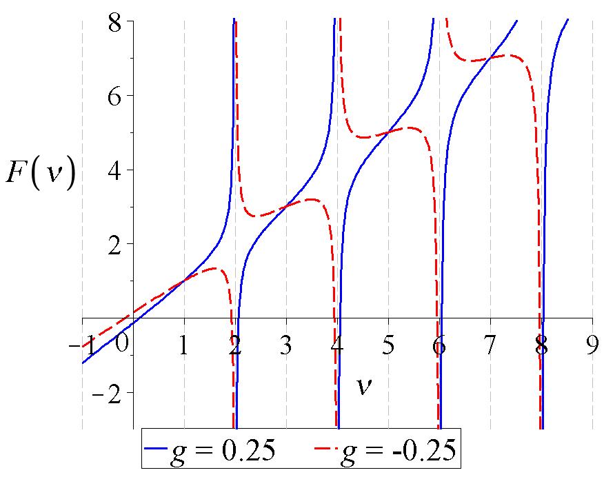
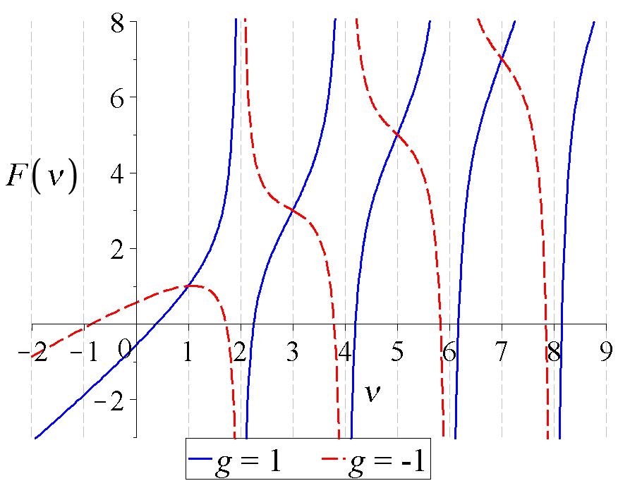
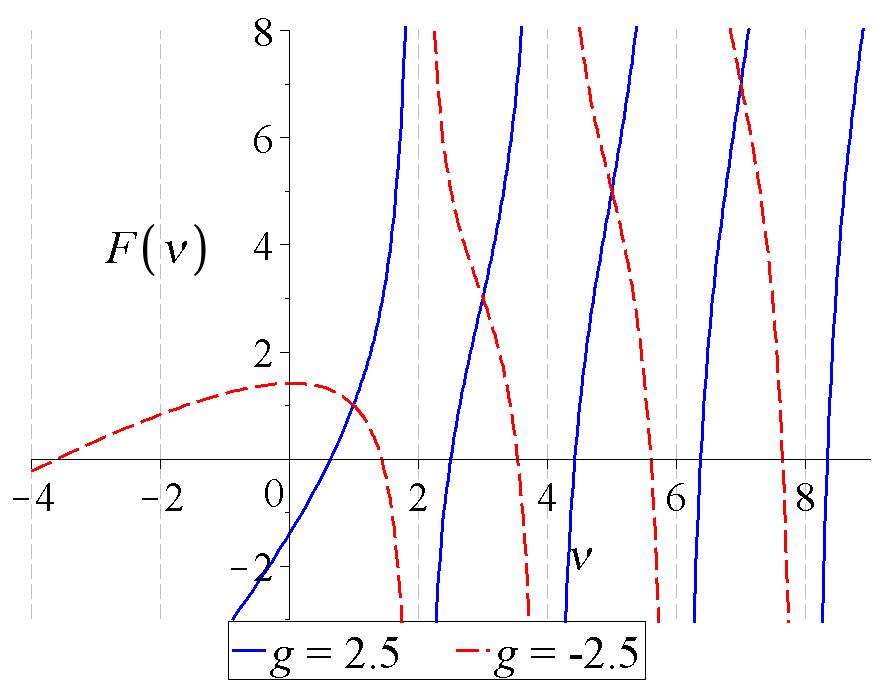
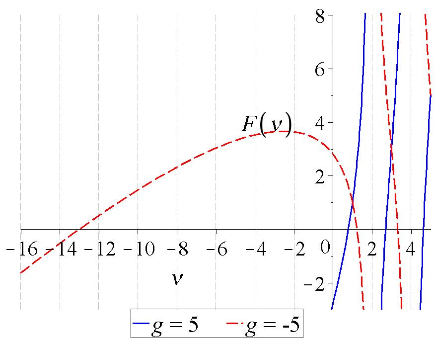
Figure 1: (color online) Graphical solution of Eq. (17), for several positive and negative values of $g$. The numerical values of $\nu$ are given in Table 1. The eigenvalues for the energy $E_{\nu}$ are given by $\nu+{\textstyle\frac{1}{2}}$ with $\nu$ the interceptions of the graphs with the $x$-axis (dashed lines refer to negative $g$, whereas solid lines refer to positive $g$).

The solution of the even parity eigenfunctions $\psi_{g}^{\rm even}(y)$ is not as simple, since these states feel the presence of the delta function at the origin. We need to find now the boundary condition the function $w(y)$ must obey at the origin. Proceeding as we did at the introductory section, we integrate Eq. (8) around $y=0$ obtaining:

$$w^{\prime}_{>}(0^{+})-w^{\prime}_{<}(0^{-})=2gw(0)\,.$$ (14)

Eq. (14) enable us to find the quantized energies of the even parity eigenstates we are seeking. Thus, the correct wave function for $\psi_{g}^{\rm even}(y)$ is $\psi_{\nu}(y)$ and not $\psi_{n}(y)$ with $n=0,2,4,\ldots$, as in the case $g=0$, for the latter wave function violates the boundary condition (14). Using the results [9, f]

$$\lim_{x\rightarrow 0^{+}}U(-\nu/2,1/2,y^{2}) = \frac{\sqrt{\pi}}{\Gamma(1/2-\nu/2)}\,,$$ (15)

$$\lim_{x\rightarrow 0^{+}}U^{\prime}(-\nu/2,1/2,y^{2}) = \frac{\nu\sqrt{\pi}}{\Gamma(1-\nu/2)}\,,$$ (16)

the eigenvalues associated with even parity eigenstates of Eq. (6) are given by the numerical solution of the transcendent equation

$$F(\nu)\equiv\nu-g\frac{\Gamma(1-\nu/2)}{\Gamma(1/2-\nu/2)}=0\,,$$ (17)

which follows from the boundary condition (14). In Fig. (1) we give the graphical solution of Eq. (17) for for $g=\pm 0.25$, $g=\pm 1.0$, $g=\pm 2.5$, and $g=\pm 5.0$, and in Table 1 the corresponding numerical values of $\nu$, for the first five even-eigenstates. As expected, the effect of the potential is to shift the eigenenergies of the even-states of the ordinary harmonic oscillator up or down in energy for positive and negative values of $g$, respectively. This effect is stronger for the low-lying eigenvalues (as we can anticipate from perturbation theory), and shifts the eigenenergies of the states $\psi_{\nu}(x)$ toward those of their lower or higher neighboring odd-states, depending on the signal of $g$. This behavior is plotted in Figure 2. In the problem we are dealing with, and contrary to the simple case of the ordinary harmonic oscillator, if $g<0$ there is also a negative energy eigenvalue, as we could have anticipated from the solution of the attractive $\delta-$function potential we have described in the introduction to this article. The absolute value of this negative energy state increases with the strength of the $\delta-$function potential and, in the limit $g\rightarrow-\infty$, the confinement imposed by the harmonic potential becomes irrelevant and the wave function transforms into the bound state given by Eq. 3 and with the same eigenenergy. Indeed, using Stirling’s formula [9, h], it is easy to prove that as $z\rightarrow\infty$, $\Gamma(z+{\textstyle\frac{1}{2}})/\Gamma(z)\rightarrow\sqrt{z}$. For $z=1+{\textstyle\frac{1}{2}}|\nu|$ this implies that as $g\rightarrow-\infty$, $g\sim\sqrt{2|\nu|}$. Since $E\sim-|\nu|\hbar\omega$ , the former result implies that

$$E_{\nu}=-g^{2}{\textstyle\frac{1}{2}}\hbar\omega=-\frac{\alpha^{2}m}{2\hbar^{2}},$$

which is the energy value we have obtain before for the simple case of an isolated attractive $\delta-$function potential.

$g\rightarrow 0$	$-0.25$	$0.25$	$-1.0$	$1.0$	$-2.5$	$2.5$	$-5.0$	$5.0$
0.0	-0.1557	0.1281	-0.8424	0.3927	-3.5865	0.6434	-12.9900	0.7961
2.0	1.9288	2.0693	1.7208	2.2546	1.4285	2.5042	1.2305	2.7003
4.0	3.9469	4.0525	3.7912	4.2002	3.5420	4.4274	3.3227	4.6364
6.0	5.9558	6.0439	5.8258	6.1699	5.6051	6.3772	5.3833	6.5887
8.0	7.9614	8.0384	7.8473	8.1501	7.6473	8.3412	7.4285	8.5509

Table 1: Eigenvalues $\nu$ associated to the even parity eigenstates $\psi_{\nu}(y)$ for several values of $g$; leftmost column corresponds to the case where $g\rightarrow 0$, which coincide with the harmonic oscillator even parity eigenvalues; the ensuing columns stand for $g=\pm 0.25$,$g=\pm 1.0$,$g=\pm 2.5$ and $g=\pm 5.0$. In between each pair of eigenvalues we also have the states associated with the odd parity eigenstates, which have eigenvalues $\nu=1,3,5,7,\ldots.$ The associated eigenenergies are given by $\epsilon_{\nu}=\nu+{\textstyle\frac{1}{2}}$

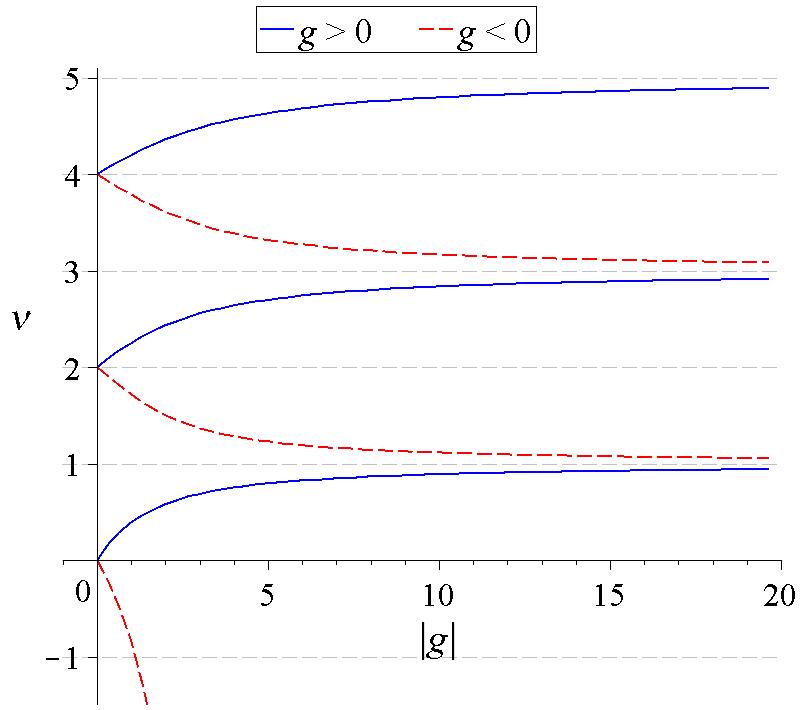
Figure 2: (color online) Graphical solution of Eq. (17), for several positive and negarive values of $g$. The numerical values of $\nu$ are given in Table 1.

Finally, in Figure 3 we plot in solid lines $|\psi_{n}(y)|^{2}$ as function of $y$ for $n=1,2,3$. In the panels (a), (b), and (c) of the same figure we also plot, in dashed lines, $|\psi_{n}(y)|^{2}$ for the wave functions that would correspond to the harmonic oscillator with $n=2$ for different positive and negative values of $g$. As $g$ increases in positive (negative) values, the corresponding value of $\nu$ approaches $\nu=3$ ($\nu=2$) making the absolute square of the wave function, $|\psi_{\nu}(x)|^{2}$, looking like the absolute square of the wave function of its odd-parity state neighbor, $|\psi_{n\pm 1}(x)|^{2}$. This doe not mean however that the two types of wave functions are the same, since they refer to orthogonal eigenstates. To make this point evident, we plot both type of states in panel (d) of Fig. 3.

It is clear from Fig. 3 the behaviour $\psi^{\prime}_{\nu}(0^{+})\neq 0$ (the number of nodes defines the order of the state). When $g\gg 1$, pairs of states (odd and even) of the harmonic oscillator with a delta-function become quasi-degenerated. Indeed, in this regime the dip of the wave function $\psi_{\nu}(y)$ at $y=0$ approaches zero, but looking at Fig. 3 it is seen by the naked eye that the two functions are orthogonal (one is even and the other is odd; this is not self-evident from the density probability graphs). The enhancement of the curvature of the wave function around $y=0$ leads to an increase of the kinetic energy and therefore to an increase of energy of the even-parity eigenstates.

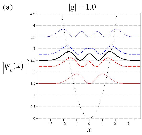
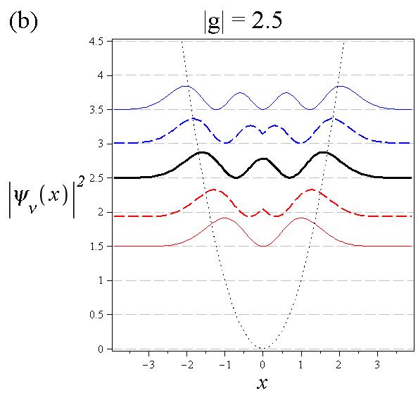
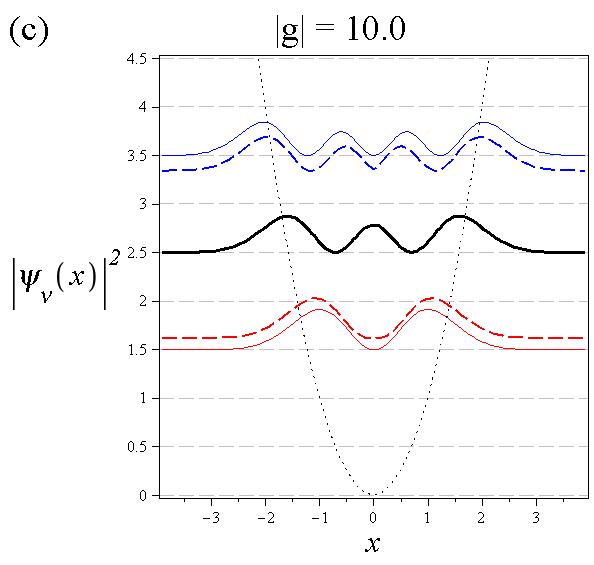
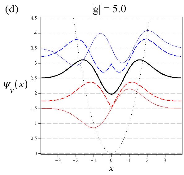
Figure 3: (color online) Panels (a), (b) and (c): absolute square values of the wave functions of the harmonic oscillator (solid lines) for (from top to bottom) $\nu=n=3,2,1$ (plotted, respectively, in blue, black and red) and for $\psi_{\nu}(x)$ (dashed lines) for $\nu$ corresponding to values of $g$ that varies from $1$ to $10$, for positive and negative values (top and bottom curves respectively). These plots show that the $|\psi_{\nu}(x)|^{2}$ curves approach the neighbors odd states. However, as it is shown in panel (d), the wave functions are quite different since the $\psi_{\nu}(x)$ are symmetrical with respect of $x$, presenting always a kink at $x=0$.

3 Conclusions

We have discussed the solution of the Schrödinger equation for the one-dimensional harmonic potential with a Dirac delta-function at the origin. The odd-parity eigenstates are given by the wave functions of the ordinary harmonic oscillator. This is obvious, since the states of the latter system are zero at the origin and therefore do not feel the presence of the delta-function. For the even parity states the solution is non-trivial. We have shown the existence of a solution of the differential equation of the harmonic oscillator that does not blow up at infinity as $e^{x^{2}/2}$ for non-integer values of $\nu$. As is well known, this solution is never mentioned in quantum mechanics textbooks for a good reason, but unfortunately that reason is, as far as we know, never discussed. Here we have shown that reason lies in the fact that its derivative at $x=0$ is finite, violating the boundary conditions imposed in the simple harmonic oscillator problem, that is, without the $\delta-$function at the origin. Nevertheless, the wave function (13) is the one we need for solving the problem (8). In our work we have computed the eigenvalues and eigenfunctions of the even parity states and made, at the same time, a little excursion to the zoo of special functions using only the famous Handbook of Mathematical Functions [6].

Note added: After the submission of this article, the work by Busch et al. [8] was brought to our attention; the latter work elaborates on top of another paper by R. K. Janev and Z. Marić [10] and, although focused on the three dimensional harmonic oscillator with a delta-function at the origin, one of the figures in Ref. [8] (Fig. 2) has the same information as our Fig. 2, albeit presented in different form. Further more, the energy eigenvalues of the zero angular momentum states are given by an equation identical to our Eq. (17) but with $1/2$ replaced by $3/2$ (for obvious reasons).

References

References

- [1] W. W. Bell, Special Functions for Scientists and Engineers, Dover, New York, 1968.
- [2] N. N. Lebedev, Special Functions and Their Applications, Dover, New York, 1972.
- [3] David J. Griffiths, Introduction to Quantum Mechanics, 2nd Ed., Person, 2005.
- [4] S. C. Bloch Introduction to Classic and Quantum Harmonic Oscillators, Wiley-Blackwell, New York, 1997.
- [5] M. Moshinsky and Yuri F. Smirnov, The Harmonic Oscillator in Modern Physics, Harwood-Academic Publishers, 2nd Ed., Amsterdam, 1996.
- [6] Milton Abramowitz and Irene Stegun, Handbook of Mathematical Functions, Dover, New York, 1965.
- [7] Michael Berry, Why are Special Functions Special?, Physics Today 54, 11 2001.
- [8] T. Busch, B. Englert, K. Rzazewski, and M. Wilkens, Two Cold Atoms in a Harmonic Trap, Foundations of Physics 28, 549 (1998).
- [9] Milton Abramowitz and Irene Stegun, Handbook of Mathematical Functions, Dover, New York, 1965. [The references given in the text are to the expressions: a)13.1.3; b)13.6.17; c)13.6.18; d)13.1.4; e)13.1.8; f)13.5.10; g)13.4.21; h)6.1.37]
- [10] R. K. Janev and Z. Marić, Perturbation of the spectrum of three-dimensional harmonic oscillator by a -potential, Phys. Lett. A 46, 313 (1974).