Some recent progress on quark pairings in dense quark and nuclear matter

Abstract

In this review article we give a brief overview on some recent progress in quark pairings in dense quark/nuclear matter mostly developed in the past five years. We focus on following aspects in particular: the BCS-BEC crossover in the CSC phase, the baryon formation and dissociation in dense quark/nuclear matter, the Ginzburg-Landau theory for three-flavor dense matter with $U_{A}$(1) anomaly, and the collective and Nambu-Goldstone modes for the spin-one CSC.

I Introduction

It is well known that fermion pairing is the underlying mechanism for superconductivity and superfluidity. In a fermionic system, the weak and attractive interaction between two fermions leads to the formation of Cooper pairs at low temperatures, which is well described by the Bardeen-Cooper-Schrieffer (BCS) theory. In strong interaction quarks and gluons are elementary particles which are described by quantum chromodynamics (QCD). There are also quark pairings called color superconductivity (CSC) first proposed in cold dense quark matter by Barrois Barrois (1977), Bailin and Love Bailin and Love (1984), and further developed by many others (for reviews, see Rajagopal and Wilczek (2000); Alford (2001); Rischke (2004); Casalbuoni and Nardulli (2004); Schafer (2003); Buballa (2005); Ren (2004); Shovkovy (2005); Huang (2005); Alford et al. (2008); Wang (2010)). However color superconducting quark matter may not be relevant in collisional experiments in the foreseeable future. The reason is that this exotic phase of matter requires extremely high baryonic densities and relatively low temperatures. In nature, such conditions may be realized in the cores of cold compact stars, i.e. in relatively old remnants of supernova explosions (for an introduction of compact star, see e.g. Schmitt (2010)). Among some major developments on quark pairings in the past decade are comprehensive studies of important CSC phases on the phase diagram Fukushima et al. (2005); Ruester et al. (2005, 2006); Blaschke et al. (2005); Sedrakian and Rischke (2009); Huang and Sedrakian (2010): the color-flavor-locking (CFL) state Alford et al. (1999); Rajagopal and Wilczek (2001), the two-flavor (2SC) state Son (1999); Pisarski and Rischke (2000); Hong et al. (2000); Wang and Rischke (2002); Schmitt et al. (2002); Nickel et al. (2006), the single flavor pairing state Schmitt et al. (2002); Schafer (2000a); Alford et al. (2003); Buballa et al. (2003); Schmitt et al. (2003); Schmitt (2005); Aguilera et al. (2005); Marhauser et al. (2007); Brauner (2008a); Pang et al. (2011); Schmitt et al. (2005, 2006); Feng et al. (2009); Blaschke et al. (2009); Feng et al. (2010); Brauner et al. (2010), mis-matched pairings Rajagopal and Wilczek (2001); Alford et al. (2001, 2004); Shovkovy and Huang (2003); Huang and Shovkovy (2004) and many other phases Schafer (2000b); Miransky and Shovkovy (2002). The construction of a theory for the CSC at weak couplings is another important progress Son (1999); Pisarski and Rischke (2000); Hong et al. (2000); Wang and Rischke (2002); Schmitt et al. (2002); Brown et al. (2000a, b, c); Schmitt et al. (2003); Hou et al. (2004); Giannakis et al. (2004).

In this review article we will give a brief overview on some recent progress in quark pairings in dense quark/nuclear matter mostly developed in the past five years. We will focus on following aspects in particular: the BCS-BEC crossover in the CSC phase, the baryon formation and dissociation in dense quark/nuclear matter, the Ginzburg-Landau theory for three-flavor dense matter with $U_{A}$(1) anomaly, and the collective and Nambu-Goldstone modes for the spin-one CSC. Random phase approximation and Dyson-Schwinger equation are used to obtain the propagating modes of diquark pairings. The BCS-BEC crossover are investigated within the boson-fermion model and the NJL-type model. The baryon formation and dissociation in different phases are studied by regarding a baryon as composed of a quark and a diquark in the NJL-type model. With a nonlocal extended NJL model one can obtain the constituent quark mass which is momentum dependent. The bubble diagrams are automatically convergent, providing an effective confinement mechanism. In a three-flavor NJL model including the axial anomaly, a low temperature critical point is found due to the coupling between chiral and diquark condensates. The collective modes in the spin-1 CSC are analyzed in the Ginzburg-Landau approach.

II BEC-BCS crossover in a relativistic boson-fermion model

The Cooper pairs are formed by two fermions at the Fermi surface in weakly attractive channel, therefore they have spatial extension called the coherence length which is much larger than the mean inter-particle distance. In a strongly coupling regime, the Cooper pairs are bound to bosonic molecules and condense in the ground state to form the so-called Bose-Einstein condensation (BEC). The Fermi surface disappears and no fermion degree of freedom remains in this situation. Although the features of BEC and BCS are very different, there is no phase transition but just a crossover between them. Recently many experimental advances have been made in cold atom system. With the help of an applied magnetic field, the effective attractive interaction between the atoms can be tuned via Feshbach resonances and the BCS-BEC crossover can be observed.

The BEC-BCS crossover in the CSC was first studied by Nishida and Abuki Nishida and Abuki (2005); Abuki (2007) with the NJL model and followed by others Deng et al. (2007); Sun et al. (2007); He and Zhuang (2007); Kitazawa et al. (2007, 2008); Brauner (2008b); Chatterjee et al. (2009); Deng et al. (2008); Sedrakian (2011). Inspired by those previously used in the context of cold fermionic atoms, one can directly extend the boson-fermion model to a relativistic version. In this case both the fermion and difermion channels are included as fundamental degrees of freedom with total fermion number density fixed. Tuning the effective interaction strength the crossover between the BEC and BCS can be studied Deng et al. (2007, 2008). In a non-relativistic system, people normally use the scattering length to characterize the strength of the attractive interaction between fermions. In the relativistic boson-fermion model, a crossover parameter $x$ is defined by the difference between the square of effective boson mass and boson chemical potential. The inverse of $x$ play the similar role of scattering length. A varying magnetic field can also lead to the relativistic BEC-BCS crossover Wang et al. (2010). Starting from any initial state at zero field, with a ultrahigh magnetic field the system always settles into a pure BCS regime.

For the NJL type model for the BCS-BEC crossover in the CSC phase Nishida and Abuki (2005); Abuki (2007); Sun et al. (2007); He and Zhuang (2007), since the fundamental degrees of freedom are fermions, the Cooper pairs are introduced with the help of bosonization procedures like Hubbard-Stratonovich transformation. Some nonperturbative tools such as random phase approximation and Dyson-Schwinger equation are needed to determine the propagating modes of the boson field. By taking the phase shift to the non-relativistic limit ($p\rightarrow 0$), an effective scattering length between fermions can be derived in relativistic case.

We review the boson-fermion model for the BCS-BEC crossover with the total fermion number density fixed Deng et al. (2007, 2008). The Lagrangian respects the global $U(1)$ symmetry, which consists of free fermion and boson parts, $\mathcal{L}_{f}$ and $\mathcal{L}_{b}$, and a Yukawa interaction part $\mathcal{L}_{I}$,

$$\mathcal{L}=\mathcal{L}_{f}+\mathcal{L}_{b}+\mathcal{L}_{I},$$ (1)

with

$$\mathcal{L}_{f} = \bar{\psi}(i\gamma^{\mu}\partial_{\mu}+\gamma^{0}\mu-m)\psi,$$

$$\mathcal{L}_{b} = |(\partial_{t}-i\mu_{b})\varphi|^{2}-|\nabla\varphi|^{2}-m_{b}^{2}|\varphi|^{2},$$

$$\mathcal{L}_{I} = g(\varphi\bar{\psi}_{C}i\gamma^{5}\psi+\varphi^{*}\bar{\psi}i\gamma^{5}\psi_{C}).$$ (2)

The fermions and bosons degrees of freedom are described by the spinor $\psi$ and the complex scalar boson field $\varphi$. The charge conjugate spinors are defined by $\psi_{C}=C\bar{\psi}^{T}$ and $\bar{\psi}_{C}=\psi^{T}C$ with $C=i\gamma^{2}\gamma^{0}$. The fermion/boson mass is denoted by $m/m_{b}$. The Lagrangian is invariant under the $U(1)_{B}$ transformation $\psi\rightarrow e^{-i\alpha}\psi$, $\varphi\rightarrow e^{2i\alpha}\varphi$. Considering a system with the total $U(1)_{B}$ charge conservation, the boson chemical potential is chosen to be twice the fermion one, $\mu_{b}=2\mu.$ Therefore, the system is in chemical equilibrium with respect to the conversion of two fermions into one boson and vice verse. This allows one to model the transition from weakly-coupled Cooper pairs made of two fermions into a molecular di-fermionic bound state, described as a boson. The bosonic field are separated into two parts as $\varphi=\varphi_{0}+\phi$, where $\varphi_{0}$ is the expectation value of the bosonic field in vacuum or the zero mode and $\phi$ is the nonzero mode. The condensation is denoted as $\Delta=2g\varphi_{0}$. The fermionic field can be rewritten in the Nambu-Gorkov (NG) basis, $\Psi=\left(\psi,\psi_{C}\right)^{T}$, $\bar{\Psi}=(\bar{\psi},\bar{\psi}_{C})$. The bosonic field can also be rewritten as $\left(\phi_{R},\phi_{I}\right)^{T}$, where $\phi_{R}$ and $\phi_{I}$ are the real and imaginary part of the complex bosonic field respectively. Then the Lagrangian can be cast into the following form

$$\mathcal{L} = \frac{1}{2}\bar{\Psi}S^{-1}\Psi+\frac{1}{2}(\phi_{R},\phi_{I})D^{-1}\left(\begin{array}[]{c}\phi_{R}\\ \phi_{I}\end{array}\right)+(\phi_{R},\phi_{I})\bar{\Psi}\left(\begin{array}[]{c}\hat{\Gamma}_{R}\\ \hat{\Gamma}_{I}\end{array}\right)\Psi+\frac{(\mu_{b}^{2}-m_{b}^{2})\Delta^{2}}{4g^{2}}.$$ (7)

Here we have re-arranged the boson-fermion interaction in the third term. The inverse tree level fermionic and bosonic propagators are denoted as $S^{-1}$ and $D^{-1}$, $\left(\hat{\Gamma}_{R},\hat{\Gamma}_{I}\right)^{T}$ is the boson-fermion vertex with $\hat{\Gamma}_{R}=i\sqrt{2}g\gamma^{5}\sigma_{1}^{NG}$ and $\hat{\Gamma}_{I}=-i\sqrt{2}g\gamma^{5}\sigma_{2}^{NG}$, where the $\sigma_{1,2}^{NG}$ are the pauli matrices in the NG basis. In the following the gap $\Delta$ is treated as real for simplicity.

With the Lagrangian density one can work out the effective potential in two levels: mean field approximation Deng et al. (2007) and the two particle irreducible (2PI) approach Deng et al. (2008). In the mean field approximation, only the condensate contribution of the bosonic field is included while the fluctuation of the field is neglected. In the 2PI approach the calculation is done in the Cornwall-Jackiw-Tomboulis (CJT) formalism Cornwall et al. (1974), in which all 2PI diagrams are counted so that the fluctuation of the bosonic field can be calculated self-consistently. The effective potential in the mean field approximation and in the 2PI approach read

$$\bar{\Gamma}_{MF}=-I(\Delta)+\frac{1}{2}\mathrm{Tr}\ln D^{-1}-\frac{1}{2}\mathrm{Tr}\ln S^{-1},$$ (8)

$$\bar{\Gamma}_{2PI} = -I(\Delta)+\frac{1}{2}\{\mathrm{Tr}\ln\mathcal{D}^{-1}+\mathrm{Tr}(D^{-1}\mathcal{D}-1)$$ (9)

$$-\mathrm{Tr}\ln\mathcal{S}^{-1}-\mathrm{Tr}(S^{-1}\mathcal{S}-1)-2\Gamma_{2PI}(\mathcal{D},\mathcal{S})\},$$

where $I(\Delta)=\frac{(\mu_{b}^{2}-m_{b}^{2})\Delta^{2}}{4g^{2}}$ is the condensate contribution. $\Gamma_{2PI}$ includes all 2PI contributions to the effective potential, which in the present case is

$$\Gamma_{2PI}\thickapprox-\frac{1}{4}\mathrm{Tr}\{\mathcal{D}_{ij}^{-1}\mathrm{Tr}[\hat{\Gamma}_{i}\mathcal{S}\hat{\Gamma}_{j}\mathcal{S}]\},$$ (10)

where $\hat{\Gamma}_{i,j}$ are the boson-fermion vertex, $i,j=R,I$ correspond to the real and imaginary components of the bosonic field, $\mathcal{D}$ and $\mathcal{S}$ are the dressed bosonic and fermionic propagators derived by the Dyson-Schwinger equations (DSE) for bosons and fermions. In the CJT formalism the DSE are given by taking derivatives of the effective potential with respect to propagators,

$$\frac{\delta\bar{\Gamma}_{2PI}}{\delta\mathcal{D}}=0, \frac{\delta\bar{\Gamma}_{2PI}}{\delta\mathcal{S}}=0,$$ (11)

which lead to the DSE,

$$\mathcal{D}^{-1} = D^{-1}-2\frac{\delta\Gamma_{2PI}}{\delta\mathcal{D}}=D^{-1}+\Pi(\mathcal{D},\mathcal{S}),$$ (12)

$$\mathcal{S}^{-1} = S^{-1}+2\frac{\delta\Gamma_{2PI}}{\delta\mathcal{S}}=S^{-1}-\Sigma(\mathcal{D},\mathcal{S}),$$ (13)

where the self-energies for bosons and fermions in the CJT formalism are given by

$$\Pi=\frac{1}{2}\mathrm{Tr}[\hat{\Gamma}_{i}\mathcal{S}\hat{\Gamma}_{j}\mathcal{S}], \Sigma(\mathcal{D},\mathcal{S})=\mathrm{Tr}[\mathcal{D}_{ij}\hat{\Gamma}_{i}\mathcal{S}\hat{\Gamma}_{j}].$$ (14)

The Rainbow-Ladder truncation is applied to the calculation for self-energies, i.e. replacing the dressed boson-fermion vertices and propagators by the bare ones. Substituting the DSE into the 2PI effective potential,

$$\bar{\Gamma}_{2PI} = -I(\Delta)+\frac{1}{2}\{\mathrm{Tr}\ln[D^{-1}(1+D\Pi)]-\mathrm{Tr}\ln[S^{-1}(1-S\Sigma)]-\mathrm{Tr}(\Sigma\mathcal{S})\}$$ (15)

$$\thickapprox -I(\Delta)+\frac{1}{2}\{\mathrm{Tr}\ln D^{-1}-\mathrm{Tr}\ln S^{-1}+\mathrm{Tr}[D\Pi(\mathcal{D},\mathcal{S})]\}.$$

In the last step an expansion in terms of self-energy has been made leading to a partial loss of self-consistence but reducing the numerical complexity. From the last line of Eq. (15), by comparing the mean-field with 2PI effective potential, one can find the beyond-mean-field contribution to the effective potential is included in $-\Gamma_{2PI}$.

From the DSE for the fermion, Eq. (13), the 11-component in the NG basis reads

$$\mathcal{S}_{11} = [(\mathcal{S}^{-1})_{11}-(\mathcal{S}^{-1})_{12}((\mathcal{S}^{-1})_{22})^{-1}(\mathcal{S}^{-1})_{21}]$$ (16)

$$= [(S^{-1})_{11}-\Sigma_{11}-(S^{-1})_{12}((S^{-1})_{22}-\Sigma_{22})^{-1}(S^{-1})_{21}]$$

$$\thickapprox [(S^{-1})_{11}-\Sigma_{11}-(S^{-1})_{12}((S^{-1})_{22})^{-1}(S^{-1})_{21}].$$

In the last line $\Sigma_{22}$ is neglected since it is sandwiched by $(S^{-1})_{12}$ and $(S^{-1})_{21}$ which are proportional to $\Delta$. $\Sigma_{11}$ is the 11-component of quark self-energy $\Sigma_{11}=\{\mathrm{Tr}[D_{ij}\hat{\Gamma}_{i}S\hat{\Gamma}_{j}]\}_{11}$. Then we have

$$-\Sigma_{11} -(S^{-1})_{12}((S^{-1})_{22})^{-1}(S^{-1})_{21}$$ (17)

$$\thickapprox -16g^{2}T\sum_{n}\sum_{e=\pm}\int\frac{d^{3}q}{(2\pi)^{3}}\frac{1}{(p_{0}+\mu_{b})^{2}-(E_{q}^{b})^{2}}$$

$$\times\frac{1}{p_{0}+q_{0}-\mu-eE_{p+q}}\gamma^{0}\Lambda_{p+q}^{-e}+\sum_{e}\frac{\Delta^{2}}{p_{0}-\mu-eE_{p}}\gamma^{0}\Lambda_{p}^{-e}$$

$$= \sum_{e}\frac{\Delta^{2}+\Delta_{pg}^{2}}{p_{0}-\mu-eE_{p}}\gamma^{0}\Lambda_{p}^{-e}.$$

The assumption $q\ll p$ is used in the second step. $E_{q}^{b}=\sqrt{q^{2}+m_{b}^{2}}$ is the boson energy in vacuum. $\Delta_{pg}$ is the pseudo-gap defined as

$$\Delta_{pg}^{2} = -16g^{2}T\sum_{n}\int\frac{d^{3}q}{(2\pi)^{3}}\frac{1}{(p_{0}+\mu_{b})^{2}-(E_{q}^{b})^{2}}$$ (18)

$$= 16g^{2}\int\frac{d^{3}q}{(2\pi)^{3}}\frac{1+f_{B}(E_{q}^{b}-\mu_{b})+f_{B}(E_{q}^{b}+\mu_{b})}{2E_{q}^{b}}$$

$$\thickapprox 16g^{2}\int\frac{d^{3}q}{(2\pi)^{3}}\frac{f_{B}(E_{q}^{b}-\mu_{b})+f_{B}(E_{q}^{b}+\mu_{b})}{2E_{q}^{b}}.$$

In the last step, the pseudo-gap are renormalized by directly removing the divergence part $1/(2E_{q}^{b})$ which comes from vacuum. From the fermionic self-energy Eq. (17), the lowest order contribution of the fluctuation is to add a pseudo-gap term $\Delta_{pg}^{2}$ to $\Delta^{2}$. Here we define the pseudo-gap as the correction to the fermion self-energy at the static limit, see Fig. 1. In the region near and above the superconductivity critical temperature $T_{c}$, the di-fermion fluctuation will contribute to the fermionic spectral density near Fermi surface by bringing in two bumps structure, but it is not a real gap since the fermionic excitation is not forbidden between the bumps. It has analytical structure from which one can compute the density of states from the di-fermion fluctuation. In the region below $T_{c}$ both the gap and pseudo-gap contribute. Here the pseudo-gap effects are approximated by $\Delta_{pg}^{2}$ for numerical simplicity. The dressed fermion propagator is also approximated by replacing $\Delta^{2}$ with $\Delta^{2}+\Delta_{pg}^{2}$.

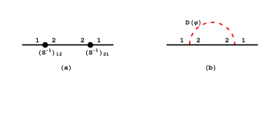
Figure 1: Diagrams for the gap and pseudo-gap. The indices 1 and 2 are for NG space.

From Eq. (14), the bosonic self-energy have four components corresponding to $i,j=I,R$. There are simple relations among them: $\Pi_{RR/II}=\Pi_{0}\pm\Pi_{1}$, $\Pi_{IR}=\Pi_{RI}=0$, where $\Pi_{0}=-8g^{2}\mathrm{Tr}[\gamma^{5}\mathcal{S}_{11}\gamma^{5}\mathcal{S}_{22}]$ is the self-energy in the normal phase ($\Delta=0$), and $\Pi_{1}=-8g^{2}\mathrm{Tr}[\gamma^{5}\mathcal{S}_{21}\gamma^{5}\mathcal{S}_{21}]$ is proportional to $\Delta^{2}$. The momentum integrals are implied in $\mathrm{Tr}$. Also we have $D_{RR}=D_{II}$ for the bare bosonic propagator. Inserting the self-energy to Eq. (10) we obtain $\Gamma_{2PI}$ as

$$\Gamma_{2PI} = -\frac{1}{2}\mathrm{Tr}[D_{RR}\Pi_{RR}]-\frac{1}{2}\mathrm{Tr}[D_{II}\Pi_{II}]=-\mathrm{Tr}(D_{RR}\Pi_{0}).$$ (19)

Then the effective potential in the mean field approximation and the 2PI approach are given by

$$\bar{\Gamma}_{MF} = -\sum_{e=\pm}\int\frac{d^{3}k}{(2\pi)^{3}}[\epsilon_{k}^{e}+2T\ln(1+e^{-\epsilon_{k}^{e}/T})]+\frac{(m_{b}^{2}-\mu_{b}^{2})\Delta^{2}}{4g^{2}}$$ (20)

$$+\frac{1}{2}\sum_{e=\pm}\int\frac{d^{3}k}{(2\pi)^{3}}[\omega_{k}^{e}+2T\ln[1-e^{-\omega_{k}^{e}/T}],$$

$$\bar{\Gamma}_{2PI} = \bar{\Gamma}_{MF}-\Gamma_{2PI},$$ (21)

where $\xi_{k}^{e}=\sqrt{k^{2}+m^{2}}-e\mu$ and $\epsilon_{k}^{e}=\sqrt{(\xi_{k}^{e})^{2}+\Delta^{2}}$ are fermionic excitation energies in normal and condensed phases respectively. In the following we use $\Omega$ to denote the thermal dynamic potential to replace the effective potential $\bar{\Gamma}$. The total charge density $n=-\frac{\partial\Omega}{\partial\mu}$ is fixed to a constant. The fermion number density for fermions, condensed/excited bosons, and the 2PI component are

$$\rho_{F} = \frac{n_{f}}{n}=\frac{2}{n}\sum_{e=\pm}\int\frac{d^{3}k}{(2\pi)^{3}}\frac{e\xi_{k}^{e}}{2\epsilon_{k}^{e}}[f_{F}(\epsilon_{k}^{e})-f_{F}(-\epsilon_{k}^{e})],$$

$$\rho_{b0} = \frac{2\mu\Delta^{2}}{ng^{2}},$$

$$\rho_{b} = \frac{2}{n}\sum_{e=\pm}\int\frac{d^{3}k}{(2\pi)^{3}}ef_{B}(E_{k}^{b}-e\mu_{b}),$$

$$\rho_{\Gamma_{2}} = \frac{1}{n}\frac{\partial\Gamma_{2PI}}{\partial\mu},$$ (22)

which satisfies

$$\rho_{F}+\rho_{b0}+\rho_{b}+\rho_{\Gamma_{2}}=1.$$ (23)

The gap equation is settled with the saddle point condition of the free energy density $F=\Omega+\mu n$, that is

$$\frac{\partial F}{\partial\Delta}=\frac{\partial\Omega}{\partial\Delta}+\frac{\partial\Omega}{\partial\mu}\frac{\partial\mu}{\partial\Delta}+n\frac{\partial\mu}{\partial\Delta}=\frac{\partial\Omega}{\partial\Delta}=0.$$ (24)

The gap $\Delta$, the chemical potential $\mu$ and the pseudo-gap $\Delta_{pg}$ can be solved simultaneously from the density and the gap equations (23,24) and the pseudo-gap equation (18). In the mean field approximation $\Gamma_{2PI}$ and $\Delta_{pg}$ are set to zero and the number of the equations is reduced to two.

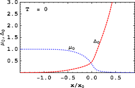
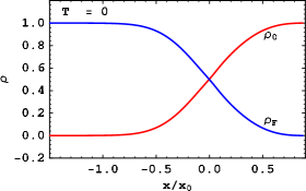
Figure 2: Left panel: the chemical potential $\mu$ (blue dotted line) and the gap $\Delta$ (red dashed line) at zero temperature as functions of $x$. Right panel: the condensed boson and fermion fractions with $x$. The units for $\mu_{0}$, $\Delta_{0}$ and $T$ are GeV.

In the mean field approximation, the renormalized boson mass $m_{br}$ can be obtained as

$$m_{b,r}^{2}=4g^{2}\frac{\partial\Omega}{\partial\Delta^{2}}|_{\Delta=T=\mu=0}=m_{b}^{2}-4g^{2}\int\frac{d^{3}k}{(2\pi)^{3}}\frac{1}{\sqrt{k^{2}+m^{2}}}.$$ (25)

In the CJT formalism to calculate the renormalized bosonic mass $m_{br}$ one should work with the bosonic DSE (12) for self-consistency. Then the pole equation in the homogeneous limit with gap set to zero is given by

$$\mathrm{det}\mathcal{D}^{-1}|_{p=\Delta=\Delta_{pg}=0}=\mathrm{det}[D^{-1}+\Pi(p_{0},\mathbf{p})]|_{\mathbf{p}=\Delta=\Delta_{pg}=0}=0,$$ (26)

with which the dressed boson mass $m_{br}$ is determined as

$$m_{br} = (p_{0}+\mu_{b})^{2}=m_{b}^{2}+\mathrm{Re}\Pi_{0}(p_{0}-i\frac{\eta}{2}),$$ (27)

$$-(p_{0}+\mu_{b})\eta-\mathrm{Im}\Pi_{0}(p_{0}-i\frac{\eta}{2})=0,$$ (28)

where $p_{0}$ is the pole position and $\eta$ is the width of the dressed boson propagator determined by the imaginary part of the pole equation (26) . The condition $\eta=0$ defines the bosonic dissociation boundary ($T^{*},\mu^{*}$). By solving the real and imaginary parts of the pole equation simultaneously, the dissociation boundary turns out to be very simple $m_{br}=2m$. In the present model the ($T^{*},\mu^{*}$) are functions of the bare boson mass $m_{b}$. From Eq. (7), with a fixed boson-fermion coupling constant $g$, $m_{b}$ is equivalent to fix the coupling constant in a pure fermionic model. Assuming the boson is stable, then we get $\eta=0$ and Eq. (27) becomes

$$m_{br}^{2}=m_{b}^{2}+\Pi_{0}(p_{0}),$$ (29)

$m_{br}$ together with the bosonic chemical potential serve as the crossover parameter $x=-\frac{m_{br}-\mu_{b}^{2}}{2g^{2}}$. The parameter $x$ can be varied from negative values with large modulus (BCS) to large positive values (BEC). In between, $x_{0}$ is the unitary limit. Therefore, $x$ behaves as the scattering length.

In Fig. 2, the calculation is done in mean field approximation for $\Delta$, $\mu$ and bosonic/fermionic charge fractions as functions of $x$. The parameters are set to $T=0$ GeV, $m=0.2$ GeV, $g=4$ and $\Lambda=1$ GeV. $x_{0}=\int\frac{d^{3}k}{(2\pi)^{3}}\frac{1}{\sqrt{k^{2}+m^{2}}}$ is an upper limit of $x$ which ensures non-negative bosonic occupation number. In the right panel of Fig. 2, the charge fraction of the thermal boson is always equal to zero since the temperature is zero. From the negative value to positive value of $x$, the system goes through a crossover from the BCS side to the BEC side.

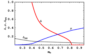
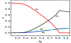
Figure 3: The fermionic chemical potential $\mu$ (blue dashed line), the gap $\Delta$ (red solid line) and pseudo-gap (black dotted line) as functions of $m_{b}$. Right panel: fractions of fermions, condensed/thermal bosons and 2PI component. The units for $m_{b}$ $\mu$, $\Delta$ and $\Delta_{pg}$ are GeV.

At high temperatures, both the condensed and thermal bosons should be considered. The results for the calculation up to 2PI are shown in Fig. 3. The parameters are chosen to be $T=0.14$ GeV, $m=0.28$ GeV, $g=1.8$ and $\Lambda=1$ GeV. With a small boson bare mass $m_{b}$ the system is in a strong coupling regime where the fermion chemical potential $\mu$ is low and the condensed bosons are dominant. When $m_{b}$ goes larger, both the gap $\Delta$ and pseudo-gap $\Delta_{pg}$ decrease while the chemical potential $\mu$ increases. The pseudo-gap $\Delta_{pg}$ is small due to a low temperature chosen here. The fraction of condensed bosons becomes smaller and the fermionic degree of freedom becomes more important. From the left panel of Fig. 3, the 2PI contribution is dominant in the large $m_{b}$ region indicating the strong interaction between fermions and bosons.

The fluctuations may change the superconducting phase transition to be of first order, such as the intrinsic fluctuating magnetic field in normal superconductors Halperin et al. (1974), or the gauge field fluctuations in color superconductors Giannakis et al. (2004), due to the fact that fluctuations bring a cubic term of the condensate to the effective potential making the Landau theory of continuous phase transition invalid. In the present case, a nonzero cubic term of $\Delta$ is generated in the bosonic fluctuation $\Gamma_{2PI}$, leading to a first order phase transition.

III Relativistic BCS-BEC crossover in Magnetic field

It is well known that an applied magnetic field can tune the BEC-BCS crossover in cold atom system, because the magnetic field can adjust the effective interaction between fermions via Feshbach resonance. In a relativistic fermion system, by applying a magnetic field with a magnitude near the energy scale of the interaction, the properties of the system will also be affected. The magnetic fields on the surface of pulsars are about $10^{12}\sim 10^{13}$ G , and for magnetars they are about $10^{14}\sim 10^{15}$ G Paczynski (1992); Duncan and Thompson (1992); Thompson and Duncan (1996). In the core the magnetic field can be even stronger. In heavy ion collision experiments at RHIC and LHC, the background magnetic field generated in non-central collisions can be about $10^{18}-10^{19}$ G at RHIC/LHC energies Kharzeev et al. (2008); Skokov et al. (2009). In the future low-energy experiments at RHIC, NICA and FAIR which is targeted to probe dense and cold nuclear matter, the magnetic field are also expected to be very strong. Such a strong magnetic may bring some significant effects to the matter, for example, the chiral magnetic effect Kharzeev et al. (2008); Fukushima et al. (2008). The strong magnetic fields have significant effects on the quark pairings in the CSC phase Ferrer et al. (2005, 2006); Ferrer and de la Incera (2007); Feng et al. (2011). Recently the magnetic field tuning of the BEC-BCS crossover has been studied Wang et al. (2010).

One can extend the boson-fermion model discussed above to study a system with oppositely charged fermions $\Psi^{T}=(\psi_{1},\psi_{2})$ and neutral scalar bosons Wang et al. (2010). An external magnetic field is also included in the model and coupled with the fermions. Then the fermion part and interaction part of Eq. (1) are

$$\mathcal{L}_{f} = \bar{\Psi}(i\gamma^{\mu}\partial_{\mu}+\mu\gamma^{0}-q\sigma_{3}\gamma^{\mu}A_{\mu}-m)\Psi,$$ (30)

$$\mathcal{L}_{I} = \varphi\bar{\Psi}_{C}(i\gamma^{5}\sigma_{2})\Psi+\varphi^{*}\bar{\Psi}(i\gamma^{5}\sigma_{2})\Psi_{C},$$ (31)

where $q$ denotes the charge of the fermion. $A_{\mu}$ is the vector potential of the external magnetic field. As discussed in Sec. II, the Lagrangian is invariant under the $\mathrm{U(1)_{B}}$ transformation $\Psi\rightarrow\Psi^{\prime}=e^{-i\alpha}\Psi$, $\varphi\rightarrow\varphi^{\prime}=e^{i2\alpha}\varphi$. Hence the simple relation $\mu_{b}=2\mu$ ensured by chemical equilibrium remains. In order to describe the BEC of these molecules, we also separate the zero-mode of the boson field $\varphi$ and replace it by its expectation value $\phi\equiv\langle\varphi\rangle$, which represents the electrically neutral difermion condensate. The mean-field effective action is then

$$I^{B}(\overline{\psi},\psi) = \frac{1}{2}\int d^{4}x\,d^{4}y\,\overline{\Psi}_{\pm}(x){\cal S}_{(\pm)}^{-1}(x,y)\Psi_{\pm}(y)+$$ (32)

$$+(4\mu^{2}-m_{b}^{2})\mid\phi\mid^{2}+\mid(\partial_{t}-2i\mu)\varphi\mid^{2}$$

$$-\mid\nabla\varphi\mid^{2}-m_{b}^{2}\mid\varphi\mid^{2},$$

where the fermion inverse propagators of the Nambu-Gorkov positive and negative charged fields $\Psi_{+}=(\psi_{2},\psi_{1C})^{T}$ and $\Psi_{-}=(\psi_{1},\psi_{2C})^{T}$ are given by

$${\cal S}_{(\pm)}^{-1}=\left(\begin{array}[]{cc}[G_{(\pm)0}^{+}]^{-1}&i\gamma^{5}\Delta^{*}\\ i\gamma^{5}\Delta&[G_{(\pm)0}^{-}]^{-1}\end{array}\right),$$ (33)

with

$$[G_{(\pm)0}^{\pm}]^{-1}(x,y)=[i\gamma^{\mu}\Pi_{\mu}^{(\pm)}-m\pm\mu\gamma^{0}]\delta^{4}(x-y),$$ (34)

and $\Pi_{\mu}^{(\pm)}=i\partial_{\mu}\pm qA_{\mu}$. Without loss of generality, the magnetic field can be chosen along the z-axis with $A^{\mu}=(0,Bx_{1},0,0)$. By using Ritus’ transformation to momentum space, the effective potential at zero temperature reads

$$\Omega = -\frac{qB}{2\pi^{2}}\sum_{e=\pm 1}\sum_{k=0}^{\infty}d(k)\int_{0}^{\infty}dp_{3}\xi_{e}+\frac{(m_{b}^{2}-4\mu^{2})\Delta^{2}}{4}+\frac{1}{4\pi^{2}}\sum_{e=\pm 1}\int_{0}^{\infty}\omega_{e}p^{2}dp,$$ (35)

in which $d(k)=(1-\frac{\delta_{k0}}{2})$ denote the spin degeneracy of the Landau levels. $k=0,1,2...$ is the Landau level (LL). The energy dispersion of fermions and bosons is given by

$$\epsilon_{e}(k) = \sqrt{(\xi_{k}-e\mu)^{2}+\Delta^{2}},\qquad e=\pm 1$$ (36)

$$\omega_{e} = \sqrt{p^{2}+m_{b}^{2}}-2e\mu,\qquad e=\pm 1,$$ (37)

respectively. $\xi_{k}=\sqrt{p_{3}^{2}+2|q|Bk+m^{2}}$ is the energy of free fermions in the magnetic field. The parameters of the model are the momentum cutoff and the fermion mass. The total fermion number density can always be chosen to be at $x=0$ where the fermion number fractions of fermions and bosons are equal. Here we choose: the momentum cutoff is chosen to be a Gaussian type $\exp[-(p_{3}^{2}+2|q|Bk)/\Lambda^{2}]$ with $\Lambda=1$GeV, and the fermion mass $m=0.2\Lambda$. With the effective potential, the gap equation $\partial\Omega/\partial\Delta=0$ and the density equation $-\partial\Omega/\partial\mu=n$ can be simultaneously solved.

In this model there are two variable parameters: the bare boson mass $m_{b}$ and the magnetic field $B$. From Fig. 2, with $B=0$ and $m_{b}$ is small the system is in BEC regime, a large $m_{b}$ corresponds to BCS regime. Varying $m_{b}$, the system makes crossovers between these two regimes. In the following the boson mass $m_{b}$ is fixed since the effect of magnetic field can be shown.

Fig. 4 shows the chemical potential, the gap and fermion number fraction of the condensate bosons and fermions as functions of $B$ with $m_{b}=0.8$ GeV Wang et al. (2010). As the magnetic field is weak on the left end of the panels, the system is in BEC regime with the condensate fraction much larger than the fermion fraction. Increasing $B$ till $\ln(qB/m^{2})\sim 0.1$, a de Haas van Alphen behavior will be present. But in this case there is only one oscillation with small amplitude on the curves for $\mu$ and $\Delta$, since the system is in the BEC regime in weak magnetic field with the gap about 73 MeV, while the de Haas van Alphen oscillation favors small $B$ and the amplitude is suppressed by a large gap. By setting a large enough value for the bare boson mass to let the system start in BCS side, by tuning the magnetic field the oscillation will be more obvious and one can find several crossovers in the fermion number fraction. Continuously increasing the magnetic field, a pure BCS state settles down on the right end of the panels. This process is a BCS-BEC crossover by varying the magnetic field, but the origin is different from that in non-relativistic case where magnetic field is used to tune the Feshbach resonance.

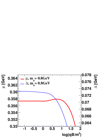
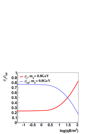
Figure 4: The fermionic chemical potential and the gap (upper panel), and fermion number fractions (lower panel) as functions of $\ln(qB/m^{2})$. Starting from the BEC side where the BEC component is much larger than the BCS component at small magnetic field on the left. The system crossover to a pure BCS state at large magnetic fields on the right.

The mechanism of the crossover can be explained by the energy dispersion of the fermion shown in Fig. 5 Wang et al. (2010). In the left panel of Fig.5, the LLs with $k<3$ contribute to the BCS component on which the minima is located at $p_{3}\neq 0$, while the one with $k=3$ contributes to the BEC one. Since the fermion energy splitting between different LLs and the density of states of each LL are all proportional to $\sqrt{eB}$, when the field increases not only the energy levels become more separated, as seen from the figure, they can also accommodate a larger number of particles. As a consequence, when the field increases, the number of occupied LLs reduces, or in other words, the magnetic field will press the fermions to lower LLs. Hence, with increasing the field the contribution from the lowest LL becomes more important and finally dominant. The higher levels shown in the middle and lower panel of Fig. 5 are likely not to contribute in strong fields. That is the reason why in a strong magnetic field the system is in the BCS regime.

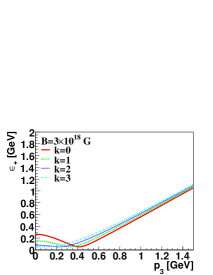
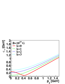
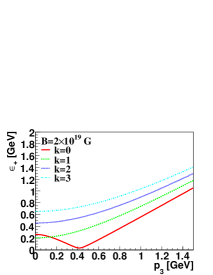
Figure 5: Positive energy component of fermion dispersion relation with fixed $m_{b}$ and $B$. The LLs $k=0,1,2,3$.

If the relativistic BCS-BEC theories discussed in the literature have any relevance for the physics of neutron stars and the future low-energy heavy ion collision experiments, we should study the effects of the magnetic field on the BCS-BEC crossover within a more realistic model, as extremely strong magnetic fields are expected to be present.

IV Diquark properties and BCS-BEC crossover in dense quark matter

The interaction between two quarks in the anti-triplet channel in color space is attractive, leading to Cooper pairs of quarks at extremely high densities and low temperatures. Due to asymptotic freedom of QCD, the interaction is weak and the Cooper pair wave function has a correlation length that exceeds the inter-particle distance. However, as the density is lowered, the interaction strength increases and the Cooper pair becomes more localized. Eventually, Cooper pairs will form tightly bound molecular diquark states, then the diquark BEC regime is settled. Since the interaction between quarks is strong, it is argued that the diquark fluctuation is large around the critical temperature $T_{c}$ and a pseudo-gap may be observed. When the temperature rises, the pseudo-gap will becomes smaller and finally disappear as the dissociation of diquark fluctuation. Recently there are some work that focus on those issues within the NJL model.

One considers a 2SC case in the NJL model. The Lagrangian reads

$$\mathcal{L}_{NJL} = \bar{\psi}(i\gamma_{\mu}\partial^{\mu}-\hat{m}_{0}+\mu)\psi+G_{s}[(\bar{\psi}\psi)^{2}+(\bar{\psi}i\gamma_{5}\mathbf{\tau}\psi)^{2}]$$ (38)

$$+G_{D}[\bar{\psi}i\gamma^{5}\tau_{2}J_{a}\psi_{C}][\bar{\psi}_{C}i\gamma^{5}\tau_{2}J_{a}\psi],$$

where $\psi$ and $\psi_{C}$ are quark field and its charge conjugate respectively. $\tau_{2}$ and $\mathbf{\tau}$ are the Pauli matrices in flavor space, and $(J_{a})_{bc}=-i\epsilon_{abc}(a=1,2,3)$ denote the antisymmetric color matrices. $G_{S}$/$G_{D}$ are coupling constants for quark-anti-quark/quark-quark channel, which together with the momentum cutoff $\Lambda$ and the bare quark mass $\hat{m}_{0}$ are the input parameters of the model. The hat of $\hat{m}_{0}$ means the bare quark mass in flavor space.

To introduce the chiral condensate and the diquark degrees of freedom, one can use the mean field approximation which is equivalent to the Hubbard-Stratonovich transformation in non-relativistic case. The diquark field can be decomposed into the condensate part $\Delta_{a}=2G_{D}\left\langle\bar{\psi}i\gamma^{5}\tau_{2}J_{a}\psi_{C}\right\rangle$ and the fluctuation part $\varphi_{a}$, then one gets $\bar{\psi}i\gamma^{5}\tau_{2}J_{a}\psi_{C}=\frac{\Delta_{a}+\varphi_{a}}{2G_{D}}$. In the 2SC phase the superconducting gap are chosen as $\Delta_{1,2}=0$ and $\Delta_{3}\neq 0$ without loss of generality. Then the Lagrangian (38) becomes

$$\mathcal{L}_{NJL} \thickapprox -\frac{1}{2}\bar{\Psi}S^{-1}\Psi-\frac{1}{4G_{D}}\sum_{a}|\Delta_{a}|^{2}-G_{s}(\sigma_{u}+\sigma_{d})^{2}$$ (39)

$$-\frac{1}{8G_{D}}(\varphi_{aR}^{2}+\varphi_{aI}^{2})+\frac{1}{2}\bar{\Psi}\varphi_{ai}\hat{\Gamma}_{ai}\Psi.$$

The quark fields can be expressed in the NG basis, $\Psi=(\psi,\psi_{C})^{T}$ and $\bar{\Psi}=(\bar{\psi},\bar{\psi}_{C})$. $\sigma_{u,d}$ are chiral condensates and can also be derived in the mean field approach. The inverse propagator then reads

$$S^{-1}=-\left(\begin{array}[]{cc}P_{\mu}\gamma^{\mu}+\mu\gamma^{5}-\hat{m}&i\gamma^{5}\tau_{2}J_{a}\Delta^{*}\\ i\gamma^{5}\tau_{2}J_{a}\Delta&P_{\mu}\gamma^{\mu}-\mu\gamma^{5}-\hat{m}\end{array}\right),$$ (40)

where the quark mass in flavor space is $\hat{m}=(m_{0}+m_{q})\cdot\mathbf{1}_{f}$ with $m_{q}$ the chiral condensate $-2G_{s}(\sigma_{u}+\sigma_{d})$. In present case only the scalar quark-quark channel is considered. The original complex diquark field has been decomposed into two real bosonic fields: the real part $\varphi_{aR}$ and the imaginary part $\varphi_{aI}$ with $\varphi_{a}=\frac{1}{\sqrt{2}}(\varphi_{aR}+i\varphi_{aI})$. The last term in Eq. (39) is a Yukawa type quark-quark-diquark vertex with the index $i=I,R$, with which the diquark dynamic properties can be studied. $\hat{\Gamma}_{aR,I}=\frac{i}{\sqrt{2}}\gamma^{5}\tau_{2}J_{a}\tau_{1,2}^{NG}$, where $\tau_{1,2}^{NG}$ are the Pauli matrices in the NG space. There are additional two tadpole terms: $\varphi_{a}\Delta^{*}$ and $\varphi_{a}^{*}\Delta$, but in a self-consistent theory all the tadpole terms should cancel themselves. One can prove that they are canceled by the tadpole terms of the one-loop diagram generated by the terms $\bar{\psi}i\gamma^{5}\tau_{2}J_{a}\psi_{C}\varphi_{a}^{*}$ and $\varphi_{a}\bar{\psi}_{C}i\gamma^{5}\tau_{2}J_{a}\psi$,

$$T^{\varphi} = T_{0}^{\varphi}+T_{1-loop}^{\varphi}$$ (41)

$$= -\frac{i}{4G_{D}}\Delta^{*}+\frac{1}{4}\int_{K}\mathrm{Tr}\left[i\gamma_{5}\tau_{2}J_{a}S_{12}\right]$$

$$\equiv 0.$$

This relation is satisfied due to the gap equation in the mean field. Similarly the tadpole terms corresponding to $\varphi_{a}^{*}$ can be proved to cancel each other. For clarity the tadpole terms are not included in the Lagrangian. The full diquark propagators are derived via the Dyson-Schwinger type equation,

$$D_{i,a}^{-1}(p_{0},\mathbf{p})=-\frac{1}{4G_{D}}-\Pi_{i,a}(p_{0},\mathbf{p}),$$ (42)

where $p_{0}=i2n\pi T$ are the Mastubara frequencies ($n=0,\pm 1,\pm 2...$) and $\Pi_{i,a}$ are the diquark self-energies, which have the following properties in the 2SC phase: $\Pi_{R/I,a}=\frac{1}{2}(\Pi_{0}^{a}\pm\Pi_{1}^{a})$, and $\Pi_{0}^{1}=\Pi_{0}^{2}\neq\Pi_{0}^{3}$, $\Pi_{1}^{a}=\delta_{a3}\Pi_{1}^{3}$. The expression for the $\Pi_{0,1}^{a}$ are

$$\Pi_{0}^{1,2} = -g^{2}\int_{K}\mathrm{Tr}[S_{22}(K)\gamma^{5}\tau_{2}J_{1,2}S_{11}(P+K)\gamma^{5}\tau_{2}J_{1,2}]$$ (43)

$$= 2\int\frac{d^{3}k}{(2\pi)^{3}}\{\frac{e_{1}^{\prime}\epsilon_{k}^{e^{\prime}}+\xi_{k}^{e^{\prime}}}{2e_{1}^{\prime}\epsilon_{k}^{e^{\prime}}}\frac{1-f(e_{1}^{\prime}\epsilon_{k}^{e^{\prime}})-f(\xi_{p+k}^{e})}{p_{0}-e_{1}^{\prime}\epsilon_{k}^{e^{\prime}}-\xi_{p+k}^{e}}$$

$$+\frac{e_{1}\epsilon_{p+k}^{e}+\xi_{p+k}^{e}}{2e_{1}\epsilon_{p+k}^{e}}\frac{1-f(\xi_{k}^{e^{\prime}})-f(e_{1}\epsilon_{p+k}^{e})}{p_{0}-\xi_{k}^{e^{\prime}}-e_{1}\epsilon_{p+k}^{e}}\}c_{k,p+k},$$

$$\Pi_{0}^{3} = -g^{2}\int_{K}\mathrm{Tr}[S_{22}(K)\gamma^{5}\tau_{2}J_{3}S_{11}(P+K)\gamma^{5}\tau_{2}J_{3}]$$ (44)

$$= 4\int\frac{d^{3}k}{(2\pi)^{3}}\frac{e_{1}^{\prime}\epsilon_{k}^{e^{\prime}}+\xi_{k}^{e^{\prime}}}{2e_{1}^{\prime}\epsilon_{k}^{e^{\prime}}}\frac{e_{1}\epsilon_{p+k}^{e}+\xi_{p+k}^{e}}{2e_{1}\epsilon_{p+k}^{e}}\frac{1-f(e_{1}^{\prime}\epsilon_{k}^{e^{\prime}})-f(e_{1}\epsilon_{p+k}^{e})}{p_{0}-e_{1}^{\prime}\epsilon_{k}^{e^{\prime}}-e_{1}\epsilon_{p+k}^{e}}c_{k,p+k},$$

$$\Pi_{1}^{1,2} = -g^{2}\int_{K}\mathrm{Tr}[S_{12}(K)\gamma^{5}\tau_{2}J_{1,2}S_{12}(P+K)\gamma^{5}\tau_{2}J_{1,2}]$$ (45)

$$= 0,$$

$$\Pi_{1}^{3} = -g^{2}\int_{K}\mathrm{Tr}[S_{12}(K)\gamma^{5}\tau_{2}J_{3}S_{12}(P+K)\gamma^{5}\tau_{2}J_{3}]$$ (46)

$$= -\int\frac{d^{3}k}{(2\pi)^{3}}\frac{\Delta_{3}^{2}}{e_{1}e_{1}^{\prime}\epsilon_{k}^{e}\epsilon_{p+k}^{e^{\prime}}}\frac{1-f(e_{1}\epsilon_{k}^{e})-f(e_{1}^{\prime}\epsilon_{p+k}^{e^{\prime}})}{p_{0}-e_{1}\epsilon_{k}^{e}-e_{1}^{\prime}\epsilon_{p+k}^{e^{\prime}}}c_{k,p+k},$$

where the quasi-quark energies are $\xi_{k}^{e}=eE_{k}-\mu$, $\epsilon_{k}^{e}=\sqrt{(\xi_{k}^{e})^{2}+\Delta^{2}}$ with $E_{k}=\sqrt{k^{2}+m_{q}^{2}}$. $c_{k,p+k}$ is the product of energy projectors, $c_{k,p+k}=[1+ee^{\prime}\frac{\mathbf{k}\cdot(\mathbf{p+k})+m_{q}^{2}}{E_{k}E_{p+k}}]$, where summation is implied over $e,e^{\prime},e_{1},e^{\prime}_{1}$.

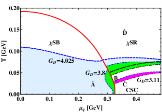
Figure 6: The phase diagram obtained within the two flavor NJL model.

With the full propagator of diquarks, one can study the stability and dissociation properties of diquarks. In Fig. 6, the red solid line separates the chiral symmetry broken phase from the symmetric phase (indicated by $\chi SB/\chi SR$); CSC denotes the color-superconducting phase. In the chiral symmetry broken phase and CSC phase, with a strong diquark coupling $G_{D}$, due to nonzero mass gap $m_{q}$ and the CSC gap $\Delta_{a}$, stable diquark poles can be found in the window $(-2m_{q},2m_{q})$ and $(-2\Delta_{a},2\Delta_{a})$ respectively in $\mathbf{p}=0$ limit. In $\chi SB$ phase (with a large $G_{D}$) and normal phase, there is a boundary below which diquark pole equations $\frac{1}{4G_{D}}+\Pi_{i,a}(p_{0},\mathbf{p})=0$ have solutions. That line is defined as the diquark dissociation boundary, see the blue dashed lines for three values of the diquark coupling constant, $G_{D}=3.11,3.8,4.025$ (in units of $\mathrm{GeV}^{-2}$) in Fig. 6. The corresponding regions in Fig. 6 are filled with light blue, green, and magenta color, respectively. These poles also exist in the CSC phases, however, for the sake of clarity there is no color in the CSC regions. The CSC phases for $G_{D}=3.11,3.8,4.025$ are bounded by the red solid line and the dash-dotted lines from bottom to top, respectively. Note that the diquark coupling constants we have chosen here are in the weak-coupling or BCS regime. As we increase $G_{D}$, Bose-Einstein condensation of diquarks can take place in the region below the dissociation lines, provided the bare quark mass is nonzero Deng et al. (2007); Kitazawa et al. (2008); Deng et al. (2008); Nishida and Abuki (2005); Sun et al. (2007); Brauner (2008b); Abuki et al. (2010); Basler and Buballa (2010). Note that in Ref. Kitazawa et al. (2008), a vanishing decay width was imposed as an additional criterion for the location of the dissociation boundary.

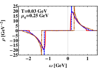
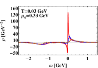
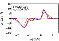
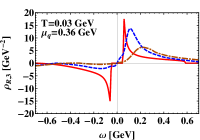
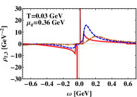
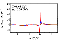
Figure 7: Spectral densities for different values of $T$ and $\mu_{q}$. The upper panels correspond to $(T,\mu_{q})=$(0.03,0.25), (0.03,0.33), (0.15,0.36) GeV, respectively. The lower panels are for $(T,\mu_{q})=(0.03,0.36)$ GeV (inside CSC phase). The indices in the spectral density refer to I,R and colors.

In Fig. 7, the diquark spectral densities are presented for four points: $A$ ($T=0.03$, $\mu=0.25$ GeV), $B$ ($T=0.03$, $\mu=0.33$ GeV), $C$ ($T=0.03$, $\mu=0.36$ GeV) and $D$ ($T=0.15$,$\mu=0.36$) in the phase diagram Fig. 6. The spectral density for diquarks is defined as following

$$\rho_{i,a}(\omega,\mathbf{p})=\frac{1}{\pi}\frac{\mathrm{Im}D_{i,a}^{-1}(\omega+i\eta,\mathbf{p})}{[\mathrm{Re}D_{i,a}^{-1}(\omega+i\eta,\mathbf{p})]^{2}+[\mathrm{Im}D_{i,a}^{-1}(\omega+i\eta,\mathbf{p})]^{2}}\;.$$ (47)

In each panel there are three curves corresponding to three momenta $|\mathbf{p}|=0,0.2,0.4$ GeV. The diquark coupling constant is chosen as a weak one $G_{D}=3.11\mathrm{GeV}^{-2}$. The upper three panels of Fig. 7 correspond to points $A$, $B$, $D$, from left to right respectively. All the six components of spectral density with indices $i=R,I$ and $a=1,2,3$ are identical outside CSC phase. At point $A$ (in $\chi SB$ phase), with a weak diquark coupling, there are only broad bumps above two times quark mass gap ($|\omega|>2m_{q}$). The point $B$ is located below the diquark dissociation boundary in normal phase, where diquarks have poles corresponding to stable diquark resonances. The point $D$ is above the dissociation boundary in the normal phase, and no diquark pole exists. The broad bumps in the diquark spectral density indicate unstable diquark resonances. The lower three panels are for $\varphi_{I}$ and $\varphi_{R}$ diquark field with color indices 1,2,3 at point $C$ in CSC region. The $I,R$ diquark field with color index 3 are gapped while the others are not. From the expressions of diquark self-energy, five Nambu-Goldstone modes are recognized, those are the $I/R$ fields with color indices $1$ and $2$, and the $I$ field with the color index $3$. They can be directly proved with the fact that the diquark pole is located at $(\omega,\mathbf{p})=0$ GeV due to the gap equations for $\Delta_{a}$. In the lower-middle (spectral density for the $\varphi_{I,3}$ field ) and lower-right panel (spectral density for the $\varphi_{I/R,1/2}$ field), one can find the five Nambu-Goldstone modes at $(\omega,\mathbf{p})=0$ GeV. The lower-left panel is for $\varphi_{R,3}$ field without Nambu-Goldstone mode.

To evaluate the thermal diquark contribution to the thermodynamic potential, Abuki has developed a method to express the potential in terms of diquark spectral density Abuki (2007). The total thermodynamic potential is decomposed into two terms $\Omega=\Omega_{MF}+\Omega_{fluc}$, where $\Omega_{MF}$ is the mean field potential and $\Omega_{fluc}$ is the thermal diquark contribution. The full diquark propagator at some coupling constant $4G_{D}={\cal{G}}$ is obtained with the dispersion relation

$$D_{i,a}^{{\cal{G}}}(i\omega_{n},\mathbf{p}) = \frac{1}{-1/{\cal{G}}-\Pi_{i,a}}=\int_{-\infty}^{\infty}d\omega\frac{\rho_{i,a}^{{\cal{G}}}(\omega,\mathbf{p})}{\omega-i\omega_{n}}.$$ (48)

The thermodynamic potential is given by

$$\Omega_{fluc} = \frac{1}{2}T\sum_{n,i,a}\int\frac{d\mathbf{p}}{(2\pi)^{3}}\log\left[\frac{1}{4G_{D}}+\Pi_{i,a}\right]-(T=\mu=0\text{ part})$$ (49)

$$= -\frac{1}{2}\int_{0}^{4G_{D}}\frac{d{\cal{G}}}{{\cal{G}}^{2}}\int\frac{d\mathbf{p}}{(2\pi)^{3}}T\sum_{n,i,a}\int_{-\infty}^{\infty}d\omega\frac{\rho_{i,a}^{{\cal{G}}}(\omega,\mathbb{p})}{\omega-i\omega_{n}}-(T=\mu=0\text{ part})$$

$$= -\frac{1}{2}\int_{0}^{4G_{D}}\frac{d{\cal{G}}}{{\cal{G}}^{2}}\int\frac{d\mathbf{p}}{(2\pi)^{3}}\int_{-\infty}^{\infty}d\omega\sum_{i,a}\rho_{i,a}^{{\cal{G}}}(\omega,\mathbb{p})[\frac{1}{2}+n_{B}(\omega)]-(T=\mu=0\text{ part}).$$

The advantage of the propagator in terms of the dispersion relation is that the summation over Matsubara frequency can be analytically performed. The fluctuation part can be decomposed into two pieces: the Nozières-Schmitt-Rink term

$$\Omega_{NSR} = -\frac{1}{2}\int_{0}^{4G_{D}}\frac{d{\cal{G}}}{{\cal{G}}^{2}}\int\frac{d\mathbf{p}}{(2\pi)^{3}}\int_{-\infty}^{\infty}d\omega\sum_{i,a}\rho_{i,a}^{{\cal{G}}}(\omega,\mathbb{p})[n_{B}(\omega)+\theta(-\omega)]$$ (50)

$$= -\frac{1}{2}\int\frac{d\mathbf{p}}{(2\pi)^{3}}\int_{-\infty}^{\infty}d\omega\sum_{i,a}\delta_{i,a}(\omega,\mathbb{p})[n_{B}(\omega)+\theta(-\omega)],$$

and the quantum fluctuation term

$$\Omega_{qfl} = -\frac{1}{2}\int_{0}^{4G_{D}}\frac{d{\cal{G}}}{{\cal{G}}^{2}}\int\frac{d\mathbf{p}}{(2\pi)^{3}}\int_{-\infty}^{\infty}d\omega\sum_{i,a}\Delta\rho_{i,a}^{{\cal{G}}}(\omega,\mathbb{p})\frac{\mathrm{sgn}(\omega)}{2}$$ (51)

$$= -\frac{1}{2}\int\frac{d\mathbf{p}}{(2\pi)^{3}}\int_{-\infty}^{\infty}\frac{d\omega}{\pi}\sum_{i,a}\Delta\delta_{i,a}(\omega,\mathbb{p})\frac{\mathrm{sgn}(\omega)}{2},$$

in which the integral over the spectral density is represented by the phase shift defined as

$$\int_{0}^{4G_{D}}\frac{d{\cal{G}}}{{\cal{G}}^{2}}\rho_{i,a}^{{\cal{G}}}=\frac{i}{2}\log\left[\frac{-\frac{1}{4G_{D}}-\Pi_{i,a}(\omega+i\eta,\mathbf{p})}{-\frac{1}{4G_{D}}-\Pi_{i,a}(\omega-i\eta,\mathbf{p})}\right]=\delta_{i,a}(\omega,\mathbf{p}).$$ (52)

Here $\Delta\rho_{i,a}^{{\cal{G}}}=\rho_{i,a}^{{\cal{G}}}-(T=\mu=0\text{ part})$ and $\Delta\delta_{i,a}=\delta_{i,a}-(T=\mu=0\text{ part})$. $n_{B}$ is the bosonic distribution function. $\Omega_{NSR}$ is the contribution from the thermal fluctuation which vanishes at zero temperature, while $\Omega_{qfl}$ remains at zero T. In further calculation the quantum fluctuation contribution is neglected, and only the thermal effect is considered. The charge conjugation is maintained without $\Omega_{qfl}$. There are two special values of $G_{D}$ which should be noticed. The first one is $1/4G_{0}=-\Pi_{i,a}(2m,\mathbf{0})|_{T=\mu=\Delta=0}$, with $G_{D}>G_{0}$ the stable diquark bound state can be found, and with $G_{D}<G_{0}$ there is only unstable diquark resonance. The diquark self-energy in the normal phase can be separated into the vacuum part and the matter part as

$$\Pi(p_{0},\mathbf{p}) = \Pi^{mat}(p_{0},\mathbf{p})+\Pi_{T=\mu=0}(p_{0}+2\mu,\mathbf{p})$$ (53)

$$= 4\int\frac{d^{3}k}{(2\pi)^{3}}\frac{1-(e+e^{\prime})/2-f(\xi_{k}^{e^{\prime}})-f(\xi_{p+k}^{e})}{p_{0}-\xi_{k}^{e^{\prime}}-\xi_{p+k}^{e}}c_{k,p+k}$$

$$+4\int\frac{d^{3}k}{(2\pi)^{3}}\frac{1-\Theta(-e^{\prime})-\Theta(-e)}{p_{0}+2\mu-e^{\prime}E_{k}-eE_{p+k}}c_{k,p+k},$$

where the first term is a convergent matter term since the integrand function contains a Fermi distribution function for positive energy. To remove the divergence in the vacuum term, the self-energy is subtracted by $\Pi(2m,\mathbf{0})$. Then one can defined a renormalized self-energy as $\Pi^{\mathrm{ren}}(p_{0},\mathbf{p})=\Pi(p_{0},\mathbf{p})-\Pi(2m,\mathbf{0})$. Meanwhile the coupling constant is renormalized as

$$-\frac{1}{4G_{R}}=\frac{1}{4G_{D}}-\frac{1}{4G_{0}},$$ (54)

where $G_{R}$ is related to the scattering length as $1/4G_{R}=m/4\pi a_{s}$ by taking the low energy limit $p=k\ll m$. The other limit for the coupling is $G_{c}=-\Pi_{i,a}(0,\mathbf{0})|_{T=\mu=\Delta=0}$. As $G_{D}$ approaching $G_{c}$ the mass of diquark bound state can become zero. If $G_{D}>G_{c}$ the vacuum becomes unstable. Considering a system with total baryonic number density fixed, one obtain with the fermion number conservation,

$$N_{tot}(\mu,T) = N_{MF}(\mu,T)+N_{NSR}(\mu,T)$$ (55)

$$= N_{MF}(\mu,T)+\frac{1}{2}\int\frac{d^{3}\mathbf{p}}{(2\pi)^{3}}\int_{-\infty}^{\infty}\frac{d\omega}{\pi}\sum_{i,a}\frac{\partial\delta_{i,a}}{\partial\mu}(\omega,\mathbb{p})[n_{B}(\omega)+\theta(-\omega)],$$

where $N_{MF}$ is the fermion number density from free quarks, the total quark number density is given by $N_{tot}=N_{c}N_{f}\frac{k_{F}^{3}}{3\pi^{2}}$ with $k_{F}$ being the effective Fermi momentum. Together with the Thouless condition

$$-\frac{1}{4G_{D}}-\Pi_{i,a}(0,\mathbf{0})=0,$$ (56)

by tuning $G_{D}$ in the range $[0,G_{0}]$ for weak couplings and in the range $[G_{0},G_{c}]$ for strong couplings, one can look at the BEC-BCS crossover along the CSC boundary $(\mu_{c},T_{c})$ with fixed $k_{F}$. Because in the CSC boundary the gap is always zero, the six components of the diquark self-energy and the phase shift in above equations with indices $i=R/I$ and $a=1,2,3$ are the same. Then the diquark number density can be evaluated as

$$N_{NSR}(\mu,T) \approx -N_{c}\int\frac{p^{2}dp}{2\pi^{2}}\int_{-\infty}^{\infty}d\omega\frac{\partial\mathrm{Re}\Pi}{\partial\mu}\rho(\omega,\mathbb{p})[n_{B}(\omega)+\theta(-\omega)].$$ (57)

When in strong couplings, $G_{R}>0$, the diquark spectral density $\rho(\omega,\mathbb{p})=\rho_{c}(\omega,\mathbb{p})+\rho_{\delta}(\omega,\mathbb{p})$ consists of two parts, the continuous part (unbound part) and the pole part (bound part), with $\rho_{\delta}=Z_{B}\delta(\omega+2\mu-E_{Bp})+Z_{\bar{B}}\delta(\omega+2\mu+E_{\bar{B}p})$ where $Z_{B/\bar{B}}=-\frac{1}{\partial\mathrm{Re}\Pi/\partial\mu}\mid_{\omega=\pm E_{B/\bar{B}p}-2\mu}$. $E_{B/\bar{B}p}$ is the energy of the diquark and anti-diquark bound state with three momentum $p$. As a consequence the diquark number density is also divided into two parts, the unbound diquark contribution $N_{un}$ and the bound diquark $N_{B}$ contribution. In the weak coupling case $G_{R}<0$, only the unbound part is left. In Fig. 8, the parameters are set to $\Lambda=0.7$ GeV, $\Lambda_{B}=0.65$ GeV, $m=0.2\Lambda$, and the total fermion number density is fixed at $k_{F}=0.2m$. With these parameters, one studies the diquark fluctuation effect near the unitary limit. The left panel shows the CSC critical temperature and chemical potential as functions of diquark normalized coupling constant. As the coupling becomes stronger, $T_{c}$ rises and $\mu_{c}$ decreases. The effect of the diquark fluctuation is found to lower $T_{c}$ and $\mu_{c}$ (solid curves) comparing to the mean field results $T_{MF}$ and $\mu_{MF}$ (dotted curves). At a very weak coupling, the CSC boundary can be well approximated by the mean field approximation. The right panel shows fermion number density fraction of quarks and diquarks. The diquark component increases with the diquark coupling constant. In the strong coupling side with $G_{R}>0$, $T_{c}$($\mu_{c}$) continuously increases (decreases) with the coupling constant. Both the free fermion fraction $N_{MF}/N_{tot}$ and unbound diquark fraction $N_{un}/N_{tot}$ decrease with the coupling constant once the effective chemical potential of the system becomes negative $\mu-m<0$, while the diquark bound state contribution becomes nonzero and finally dominant.

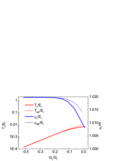
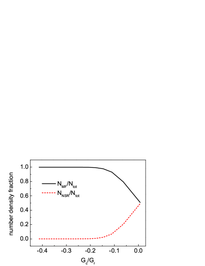
Figure 8: $T_{c}/E_{F}$ and $\mu_{c}/m$ (left panel) and number density fraction (right panel) as as functions of normalized diquark coupling constant $G_{c}/G_{r}$. Here $T_{c}$ and $\mu_{c}$ are the CSC critical temperature and chemical potential respectively.

In this section, we summarize recent results on the diquark spectral densities in different regions of the phase diagram. The quark mass and CSC gap serve as boundaries for stable diquarks. In the 2SC phase, there are gap structures in the spectral density of the thermal diquark with red and green colors. The infinite peaks at $(\omega,\mathbf{p})=(0,\mathbf{0})$ GeV indicate five Goldstone modes. In the NJL model, the scattering length $a_{s}$ of fermions can be determined by taking the non-relativistic limit for the $T$ matrix, which is an advantage in comparison with the boson-fermion model beyond leading order calculation. Considering a total baryonic number density conserved system, tuning the scattering length along the CSC boundary where the Thouless condition is satisfied, the boundary of the CSC and the number density fraction of free quarks and diquarks are calculated. When the $1/a_{s}$ is negative and small, the diquark contribution to the number density is negligible and the system is in the pure BCS regime. The diquark unstable resonance has a remarkable contribution when the absolute value of the effective chemical potential is small. When $1/a_{s}$ is positive, the diquark bound state will form. Once the effective chemical potential becomes negative, increasing $1/a_{s}$ the number density fraction of diquark bound states becomes nonzero and quickly dominates and the system settles in a deep BEC regime.

V Baryon as quark-diquark collective modes

Baryon can be studied as a bound state of three constituent quarks Oettel et al. (2002, 2000); Cloet et al. (2005); Eichmann et al. (2008, 2009, 2010). Quarks and gluons carrying color charges are confined inside baryons and mesons. The static properties of baryons in vacuum can be studied with the relativistic Faddeev equation Pepin et al. (2000); Ishii et al. (1995). In this approach, the baryon is assumed to be stable with a separable form of the T- matrix. The original Faddeev equation can be reduced to the Bethe-Salpeter equation (BSE), which is an eigen-equation for the baryonic vertex. But with a nonzero temperature and baryon density, the Faddeev equation or the BSE is hard to solve numerically. The way around is to take the static approximation for the intermediate quark propagator in the Faddeev equation. Then the baryon can be studied at nonzero temperature by a two step process: first, the thermal diquark propagator is simulated by the Dyson-Schwinger equation, and second, the diquark is coupled with another quark to form a baryon. In previous works, the diquark is always assumed to be stable, but this is not necessarily true. Baryon can be a bound state of a quark and an unstable diquark, which is like a borromean state Zhukov et al. (1993) in nuclear and atom physics.

To add the baryon field into the Lagrangian (39), a coupling term of the quark-quark-diquark-diquark is introduced as

$${\cal L}_{B} = G_{B}\varphi_{a}^{\dagger}\bar{\psi}_{a}\psi_{b}\varphi_{b}$$ (58)

$$\simeq -\frac{1}{2G_{B}}\overline{\mathbf{B}}\mathbf{B}+\frac{1}{2}\overline{\mathbf{B}}\widehat{\Gamma}_{Bi}\Psi_{a}\varphi_{ai}+\frac{1}{2}\varphi_{ai}\overline{\Psi}_{a}\widehat{\Gamma}_{Bi}^{*}\mathbf{B}\;.$$

Here, $\psi_{a}\varphi_{a}=\left\langle\psi_{a}\varphi_{a}\right\rangle+\beta_{a}$, and the baryonic field is defined as $B=G_{B}\left\langle\psi_{a}\varphi_{a}\right\rangle$. The terms of order $O(\beta_{a}^{2})$ is neglected. Actually this is equivalent to take the static approximation in Faddeev equation. The baryonic fields in the NG basis are then denoted by $\mathbf{B}=(B,B_{c})^{T}$ and $\overline{\mathbf{B}}=(\overline{B},\overline{B}_{c})$. The baryon-quark-diquark vertices are $\widehat{\Gamma}_{BR}=\frac{1}{\sqrt{2}}1_{NG}$ and $\widehat{\Gamma}_{BI}=i\frac{1}{\sqrt{2}}\tau_{3}^{NG}$, respectively. The sum of the Lagrangians (39) and (58) is the starting point for the further treatment.

The 11-component in the NG space of the inverse baryon propagator is $S_{B}^{-1}=-1/(2G_{B})-\Sigma$, where

$$\Sigma(P)=-\frac{1}{4}\sum_{a}\int_{K}S_{11}^{a}(P-K)[D_{R,a}(K)+D_{I,a}(K)]$$ (59)

is the 11-component of the baryon self-energy. The quark propagator in the NG space, $S_{11}^{a}$, is diagonal in color space. In presence of a non-vanishing diquark condensate, $S_{11}^{1}=S_{11}^{2}\neq S_{11}^{3}$. If the diquark condensate vanishes, $S_{11}^{1}=S_{11}^{2}=S_{11}^{3}$ and $D_{R,a}=D_{I,b}$ for any $a,b$. Inserting the spectral density form of the diquark full propagator Eq. (48) into Eq. (59), the summation over Matsubara frequency can be handled. Then the positive energy component of the baryon full propagator can be extracted with energy projectors, $S_{B,+}^{-1}(p_{0},\mathbf{p}=\mathbf{0})=\frac{1}{2}\mathrm{Tr}\left[S_{B}^{-1}\Lambda_{\mathbf{p=0}}^{+}\gamma^{0}\right]$, where $\Lambda_{\mathbf{p}}^{s}$ is the energy projector $\Lambda_{\mathbf{p}}^{s}=\frac{1}{2}\left[1+s\left(\gamma_{0}\gamma\cdot\mathbf{p}+\gamma_{0}M_{B}\right)/E_{p}\right]$, with $E_{p}=\sqrt{p^{2}+M_{B}^{2}}$ and $s=\pm 1$. In the homogeneous limit, $\mathbf{p}=\mathbf{0}$, the energy projector assumes a simple form, $\Lambda_{\mathbf{p=0}}^{s}=\frac{1}{2}(1+s\gamma_{0})$, which is independent of $M_{B}$. The full expression of the positive energy component of the baryon propagator is,

$$\mathcal{S}_{B,+}^{-1}(l_{0},\mathbf{0}) = \frac{1}{2}\mathrm{Tr}\left\{[-1/(2G_{B})-\Sigma^{R}]\Lambda_{+}^{\mathbf{0}}\gamma^{0}\right\}$$ (60)

$$= -1/(2G_{B})+\int\frac{p^{2}dp}{4\pi^{2}}\int_{-\infty}^{\infty}\frac{d\omega}{\pi}\{4\rho_{R/I}^{1}(\omega,\mathbf{p})\frac{e_{1}\epsilon_{\mathbf{p}}^{e}+\xi_{\mathbf{p}}^{e}}{2e_{1}\epsilon_{\mathbf{p}}^{e}}\frac{f(e_{1}\epsilon_{\mathbf{p}}^{e})+n(\omega)}{l_{0}-\omega+e_{1}\epsilon_{\mathbf{p}}^{e}}$$

$$+[\rho_{R}^{3}(\omega,\mathbf{p})+\rho_{I}^{3}(\omega,\mathbf{p})]\frac{f(\xi_{\mathbf{p}}^{e})+n(\omega)}{l_{0}-\omega+\xi_{\mathbf{p}}^{e}}\}(1+e\frac{m_{q}}{E_{\mathbf{p}}}).$$

where summation is implied over $e,e_{1}$.

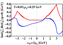
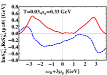
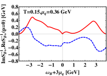
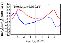
Figure 9: The real (blue dashed) and imaginary (red solid) parts of the inverse propagators for baryons as functions of energy $\omega$ at different $T$ and $\mu_{q}$. From top to bottom, the first panel: $T=0.03$ and $\mu_{q}=0.25$ (point A). The second panel: $T=0.03$ and $\mu_{q}=0.33$ (point B). The third panel: $T=0.15$ and $\mu_{q}=0.36$ (point D). The fourth panel: $T=0.03$ and $\mu_{q}=0.36$ (point C). All units in GeV.

Fig. 9 shows the real and imaginary parts of the inverse retarded Greens function for baryons (positive energy component), again at points A,B,C, and D in the phase diagram of Fig. 6. The diquark coupling constant is taken to be weak, $G_{D}=3.11$ GeV^-2. The constant $G_{B}=10.04$ GeV^-1 is chosen to make the baryon mass of $0.94$ GeV in vacuum. In the chiral symmetry broken phase with $m_{q}\neq 0$ and $\Delta=0$ (point A), there are no diquark condensates or resonances but stable baryon resonances: in the upper-left panel, one can see that $\mathrm{Re}S_{B+}^{-1}(\omega_{B},\mathbf{0})=0$ has a solution at $\omega_{B}+3\mu_{q}\approx 0.94$ GeV, i.e., close to the nucleon rest mass. There is a region of $\omega_{B}\in[-3(m_{q}+\mu_{q}),3(m_{q}-\mu_{q})]$ or $M_{B}\in[-3m_{q},3m_{q}]$, where the imaginary part $\mathrm{Im}S_{B+}^{-1}(\omega_{B},\mathbf{0})$ is very small (smaller than $10^{-6}$ GeV) in the homogeneous limit. The position is just inside this region, i.e., $M_{B}<3m_{q}$: the baryon weighs less than its constituents. It is therefore stable, although its constituents by themselves are unbound, like in a Borromean state in atomic or nuclear physics. The upper-right panel shows the case with diquark resonances but outside the CSC phase (point B). There is no positive energy baryon pole in this case. In the region of higher temperatures and quark chemical potentials where chiral symmetry is restored and where there are neither diquark condensates nor resonances (point D), there are also no baryon resonances and the absolute value of $\mathrm{Im}S_{B+}^{-1}$ is very large. This case is shown in the third panel. In the CSC phase (point C), there are baryon poles but with nonzero imaginary parts, indicating unstable baryon resonances, as shown in the fourth panel.

There are a lot of works using the simplified Faddeev equation by static approximation to study baryon properties in vacuum and nuclear matter, see, for example, Ref. Bentz and Thomas (2001); Bentz et al. (2003). But the issues the authors focus on are different. To give the diquark propagator they used the proper time regularization method which introduces an effective confinement, but the method is not applicable to nonzero temperature case. The diquark T-matrix is approximated by the constant term $\frac{1}{4G_{D}}$ plus the pole terms, which is equivalent to the assumption of a stable form diquark propagator, while as presented in Fig. 9, the baryon can also be formed by an unstable diquark and a quark. The pole approximation for the diquark propagator will miss some of important physics like Borromean state. In further calculation the physics mass of baryon bound state or baryon resonance can be obtained at any given $T$ and $\mu$ on the phase diagram based on the mean field approximation by the NJL. In the present approach, at low temperatures, the baryon mass have only a slight decrease when the chemical potential rises, but in Ref. Bentz and Thomas (2001); Bentz et al. (2003) baryon mass decreases significantly. The reason is that the vector meson is not included and a large baryon number density could not be obtained by increasing the chemical potential. Also the confinement mechanism at finite temperatures should be incorporated. In Ref. Gastineau and Aichelin (2005), the static approximation and the stable diquark are used. The authors considered a three-flavor NJL model, where the baryon mass is found to decrease by $25\%$ at normal nuclear matter densities. These issues can also be considered in the present framework.

In summary, diquark propagating modes are derived with an NJL-type model in different regions of the phase diagram of strongly interacting matter. Baryon formation and dissociation in dense nuclear and quark matter is then studied via the baryon poles and spectral densities, incorporating the previously obtained diquark propagator. The stable baryon resonances with zero width are present in the phase of broken chiral symmetry, where the diquarks could be an unstable resonance. This indicates that the baryon can be a Borromean like bound state. There are no baryon poles in the chirally symmetric phase. In the CSC phase, baryon poles exist, but they are found to be unstable due to a sizable width.

VI Nonlocal extension of NJL model and its applications

The NJL-type model applied to quarks is a successful schematic effective theory for QCD, in which the interaction between quarks are described by point-like couplings. The model can be used to study the spontaneous chiral symmetry breaking and quark pairings. But the basic version of the NJL model have some shortcomings. For example, the NJL model can not exhibit confinement as in QCD. The other one is the constituent quark mass is independent of momentum which is in conflict with the lattice data and the Dyson-Schwinger equation from QCD. The second point can be studied by a nonlocal extension of the point-like coupling in the NJL model. The nonlocal quark current reads,

$$J_{M}=\int d^{4}x_{1}d^{4}x_{2}f(x_{1})f(x_{2})\bar{q}(x-x_{1})\Gamma_{M}q(x+x_{2}),$$ (61)

in which $M=\sigma,\pi$ stand for the scalar meson and the pion. $\Gamma_{\sigma/\pi}$ are $1$ and $\gamma^{5}\tau_{a}$ respectively with flavor indices $a=1,2,3$. $f$ is a form factor in momentum space, usually taken as a Gaussian type $f^{2}(p^{2})=\exp(-p^{2}/\Lambda^{2})$. The basic NJL model is non-renormalizable and some form of ultraviolet regularization is necessary with a cutoff parameter which is a part of the model. But in the nonlocal NJL model the momentum integration are automatically convergent in the loop diagrams and no additional regularization method is needed Radzhabov et al. (2011).

The parameters of the model including the coupling constant $G$, the quark current mass $m_{c}$ and the momentum cutoff $\Lambda$ are determined by fitting the pion mass $M_{\pi}$ and the decay constant $f_{\pi}$ in vacuum. The meson sectors are defined by introducing the auxiliary scalar field $\tilde{\sigma}=G\left<J_{\sigma}(x)\right>$ and pseudo-scalar $\pi^{a}=G\left<J_{\pi}(x)\right>$. The dressed quark propagator in the mean field approximation is determined by the following equation

$$S(p)^{-1} = \not{p}-m_{c}-\Sigma(p),$$ (62)

where $\Sigma(p)$ is the self-energy which turn out to be $\Sigma(p)=m_{d}f^{2}(p^{2})$, with $m_{d}=iG\Gamma_{M}\int_{K}\mathrm{Tr}[\Gamma_{M}S(k)f^{2}(k^{2})]$ a momentum independent constant serving as an order parameter for the dynamical chiral phase transition. The 1PI diagram of the self-energy vanishes due to the integration for $x_{1},x_{2}$ goes from $-\infty$ to $+\infty$. Comparing to the classic NJL model, the constituent quark mass now depends on the three momentum by a Gaussian factor. In Dyson-Schwinger equation from QCD, the dressed quark propagator has the form $S(p)=Z(p^{2})[\not{p}-M(p^{2})]$. The renormalization function $Z(p^{2})$ can also be obtained in the nonlocal NJL framework by considering the thermal meson correlation beyond mean field approximation Radzhabov et al. (2011).

The meson propagator is given by RPA for the Bethe-Salpeter equation $D^{M-1}(p)=-G^{-1}+\Pi^{M}(p)$, with $\Pi^{M}(p)$ polarization function in the mean field approximation Radzhabov et al. (2011),

$$\Pi^{M}(p)=i\int_{K}f^{2}[(k+p/2)^{2}]f^{2}[(k-p/2)^{2}]\mathrm{Tr}[S(k+p/2)\Gamma_{M}S(k-p/2)\Gamma_{M}].$$ (63)

The pion mass is obtained by the pole condition $-G^{-1}+\Pi^{\pi}(p^{2}=m_{\pi}^{2})=0$. Then the quasi-particle propagator can be written as $D^{\pi}(p)=\frac{g_{\pi}^{2}}{p^{2}-m_{\pi}^{2}}$ with $g_{\pi}=\frac{1}{\partial{\Pi^{\pi}(p)}/\partial p^{2}}\mid_{p^{2}=m_{\pi}^{2}}$.

To calculate the pion weak decay constant, the weak current is introduced by a delocalization procedure for the quark fields Radzhabov et al. (2011), that is

$$q(y)\rightarrow Q(x,y)=E(x,y)q(y),$$ (64)

where $E(x,y)=\mathcal{P}\exp{i\int_{x}^{y}dz^{\mu}[\mathcal{V}_{\mu}^{a}(z)+\mathcal{A}_{\mu}^{a}(z)\gamma^{5}]T^{a}}$ is the Schwinger phase factor, $\mathcal{V}_{\mu}^{a}(z)$ and $\mathcal{A}_{\mu}^{a}(z)$ are vector and axial-vector gauge fields respectively. The nonlocal current is modified as

$$J_{M}=\int d^{4}x_{1}d^{4}x_{2}f(x_{1})f(x_{2})\bar{Q}(x-x_{1},x)\Gamma_{M}Q(x,x+x_{2}).$$ (65)

Then the weak vertices are introduced in the present nonlocal NJL model of two types: the weak current coupled with a quark $\Gamma^{5}$ and the weak current coupled with the quark meson vertex $\Gamma^{5M}$. Both give rise to the bubble diagrams which contribute to pion weak decay.

The nonlocal extension of the quark NJL model is inspired and therefore reflects some important features of QCD. The momentum dependence of the constituent quark mass can be considered and the original sharp momentum cutoff is replaced by a smooth one. Then all the loop diagrams are automatically convergent and hence the cutoff dependence of the model is highly weaken. The last point can be looked at from the calculation of the meson loop effect in the $1/N_{c}$ expansion. In the nonlocal study Radzhabov et al. (2011), the next to leading order contribution to the quark condensate turn out to be positive in vacuum, in contrast to the result obtained from the local NJL model Oertel et al. (2001), in which the beyond mean field correction is a nonlinear function of the momentum cutoff $\Lambda_{M}$.

VII Ginzburg-Landau effective theory in three-flavor dense quark matter with axial anomaly

The QCD phases in high density regime are controlled by the chiral and diquark condensates $\phi=\left\langle\overline{q}q\right\rangle$ and $d=\left\langle qq\right\rangle$. The interplay between the Nambu-Goldstone (NG) and color superconducting (CSC) phases can be described in an model-independent way by the Ginzburg-Landau (GL) theory Matsuura et al. (2004); Giannakis and Ren (2002). It has been predicted in the GL theory that a new critical point and smooth crossover arise from the coupling between chiral and diquark condensates induced by axial anomaly at the low temperature in the QCD phase diagram Hatsuda et al. (2006); Yamamoto et al. (2007); Schmitt et al. (2011). Such a coupling is also related to the continuity between the quark and hadronic matter Schafer and Wilczek (1999). The new critical point can also be confirmed in the three-flavor NJL model with axial anomaly Steiner (2005); Abuki et al. (2010); Zhang and Kunihiro (2011).

The form of the GL free energy to the sixth order in the fields can be constrained by the symmetry,

$$\mathcal{G}=SU(3)_{L}\otimes SU(3)_{R}\otimes U(1)_{B}\otimes U(1)_{A}\otimes SU(3)_{C}$$ (66)

where subscripts $L$, $R$, $B$, $A$ and $C$ stand for left-handed flavor, right-handed flavor, baryon number, axial charge, and color symmetry. The left-handed and right-handed quark fields transformed under $\mathcal{G}$ as

$$q_{\lambda} \rightarrow e^{-i\lambda\theta_{A}}e^{-i\theta_{B}}V_{\lambda}V_{C}q_{\lambda},$$ (67)

where $\lambda=L(+),R(-)$, $V_{L/R/C}$ are rotational matrices of $SU(3)_{L/R/C}$, and $\theta_{A/B}$ are rotational angles of $U(1)_{A/B}$.

The chiral fields are defined and transformed as

$$\phi_{ij} \sim \left\langle\overline{q}_{R\alpha}^{j}q_{L\alpha}^{i}\right\rangle,$$

$$\phi \rightarrow e^{-2i\theta_{A}}V_{L}\phi V_{R}^{\dagger},$$ (68)

where $i,j$ denote the flavor indices and $\alpha$ denotes the color indices. We see that $\phi$ is invariant under $Z(2)_{A}\subset U(1)_{A}$. Then we have transformation rules for these field quantities,

$$\phi\phi^{\dagger} \rightarrow V_{L}\phi\phi^{\dagger}V_{L}^{\dagger},$$

$$\phi^{\dagger}\phi \rightarrow V_{R}\phi\phi^{\dagger}V_{R}^{\dagger},$$

$$\det\phi \rightarrow e^{-6i\theta_{A}}\det\phi.$$ (69)

We see that $\det\phi$ is invariant under $Z(6)_{A}\subset U(1)_{A}$.

The diquark fields are defined as

$$\left(d_{\lambda}\right)_{i\alpha} \sim \epsilon_{\alpha\beta\gamma}\epsilon_{ijk}\left\langle\left(\overline{q}_{\lambda}\right)_{\beta}^{j}\left(q_{C\lambda}\right)_{\gamma}^{k}\right\rangle=\epsilon_{\alpha\beta\gamma}\epsilon_{ijk}\left\langle\left(\overline{q}_{\lambda}\right)_{\beta}^{j}C\left(\overline{q}_{\lambda}^{T}\right)_{\gamma}^{k}\right\rangle,$$

$$\left(d_{\lambda}^{\dagger}\right)_{\alpha i} \sim \epsilon_{\alpha\beta\gamma}\epsilon_{ijk}\left\langle\left(\overline{q}_{C\lambda}\right)_{\beta}^{j}\left(q_{\lambda}\right)_{\gamma}^{k}\right\rangle=\epsilon_{\alpha\beta\gamma}\epsilon_{ijk}\left\langle\left(q_{\lambda}^{T}\right)_{\beta}^{j}C\left(q_{\lambda}\right)_{\gamma}^{k}\right\rangle,$$ (70)

where $C=i\gamma^{2}\gamma_{0}$. Under $\mathcal{G}$, the diquark fields transform as

$$d_{\lambda} \rightarrow e^{2i\lambda\theta_{A}}e^{2i\theta_{B}}V_{\lambda}d_{\lambda}V_{C}^{T},$$

$$d_{\lambda}^{\dagger} \rightarrow e^{-2i\lambda\theta_{A}}e^{-2i\theta_{B}}V_{C}^{*}d_{\lambda}^{\dagger}V_{\lambda}^{\dagger}.$$ (71)

The color singlet quantities in diquark fields transform as

$$d_{\lambda}d_{\lambda}^{\dagger} \rightarrow V_{\lambda}d_{\lambda}d_{\lambda}^{\dagger}V_{\lambda}^{\dagger},$$

$$d_{\lambda}d_{-\lambda}^{\dagger} \rightarrow e^{4i\lambda\theta_{A}}V_{\lambda}d_{\lambda}d_{-\lambda}^{\dagger}V_{-\lambda}^{\dagger},$$

$$\det d_{\lambda} \rightarrow e^{6i\lambda\theta_{A}}e^{6i\theta_{B}}\det d_{\lambda}.$$ (72)

Then the most general form of the GL free energy which is invariant under the transformation of $\mathcal{G}$ read

$$\Omega(\phi,d_{L},d_{R}) = \Omega_{\chi}(\phi)+\Omega_{d}(d_{L},d_{R})+\Omega_{\chi d}(\phi,d_{L},d_{R}),$$

$$\Omega_{\chi}(\phi) = \frac{a_{0}}{2}\mathrm{Tr}\phi^{\dagger}\phi+\frac{b_{1}}{4!}(\mathrm{Tr}\phi^{\dagger}\phi)^{2}+\frac{b_{1}}{4!}\mathrm{Tr}(\phi^{\dagger}\phi)^{2}-\frac{c_{0}}{2}(\det\phi+\det\phi^{\dagger})$$

$$\Omega_{d}(d_{L},d_{R}) = \alpha_{0}\mathrm{Tr}[d_{L}d_{L}^{\dagger}+d_{R}d_{R}^{\dagger}]+\beta_{1}([\mathrm{Tr}(d_{L}d_{L}^{\dagger})]^{2}+[\mathrm{Tr}(d_{R}d_{R}^{\dagger})]^{2})$$

$$+\beta_{2}[\mathrm{Tr}(d_{L}d_{L}^{\dagger})^{2}+\mathrm{Tr}(d_{R}d_{R}^{\dagger})^{2}]+\beta_{3}\mathrm{Tr}[(d_{R}d_{L}^{\dagger})(d_{L}d_{R}^{\dagger})]$$

$$+\beta_{4}\mathrm{Tr}(d_{L}d_{L}^{\dagger})\mathrm{Tr}(d_{R}d_{R}^{\dagger}),$$

$$\Omega_{\chi d}(\phi,d_{L},d_{R}) = \gamma_{1}\mathrm{Tr}(d_{R}d_{L}^{\dagger}\phi+d_{L}d_{R}^{\dagger}\phi^{\dagger})+\lambda_{1}\mathrm{Tr}(d_{L}d_{L}^{\dagger}\phi\phi^{\dagger}+d_{R}d_{R}^{\dagger}\phi^{\dagger}\phi)$$ (73)

$$+\lambda_{2}\mathrm{Tr}(d_{L}d_{L}^{\dagger}+d_{R}d_{R}^{\dagger})\cdot\mathrm{Tr}(\phi^{\dagger}\phi)+\lambda_{3}[\det\phi\cdot\mathrm{Tr}(d_{L}d_{R}^{\dagger}\phi^{\dagger})+H.c.].$$

For three massless flavor case, the most symmetric condensate is in the form

$$\phi = \mathrm{diag}(\sigma,\sigma,\sigma),$$

$$d_{L} = -d_{R}=\mathrm{diag}(d,d,d).$$ (74)

Then the GL free energy reads,

$$\Omega_{3F} = \frac{a}{2}\sigma^{2}-\frac{c}{3}\sigma^{3}+\frac{b}{4}\sigma^{4}+\frac{f}{6}\sigma^{6}$$ (75)

$$+\frac{\alpha}{2}d^{2}+\frac{\beta}{4}d^{4}-\gamma d^{2}\sigma+\lambda d^{2}\sigma^{2},$$

where coefficients $a,b,c,f,\alpha\beta\gamma\lambda$ come from those in Eq. (73). Here $a,\alpha$ are two essential parameters to drive the phase transition. $b$ can change sign with $T,\mu$, so a positive $\sigma^{6}$ term ($f>0$) is introduced to stabilize the system for negative $b$. $\beta$ is positive definite from effective theories and weak-coupling QCD. The $\sigma^{3}$ and $d^{2}\sigma$ terms are from axial anomaly so the coefficients $c$ and $\gamma$ are related and are all positive. $\lambda$ is also positive from the NJL model and weak-coupling QCD.

There are four phases: the normal (NOR) phase with $\sigma=0$ and $d=0$, the CSC phase with $\sigma=0$ and $d\neq 0$, the Nambu-Goldstone (NG) phase with $\sigma\neq 0$ and $d=0$, and the coexistence (COE) phase with $\sigma\neq 0$ and $d\neq 0$. The phases at a specific set of parameters can be determined by comparing the global minima of the free energies $\Omega_{NOR}$, $\Omega_{CSC}$, $\Omega_{NG}$ and $\Omega_{COE}$. From NOR or CSC phase with $\sigma=0$ to the NG phase with $\sigma\neq 0$, there is a first-order transition phase for the chiral symmetry breaking or restoration. The transition between the NOR phase with $d=0$ and the CSC phase $d\neq 0$ is a second-order one with a discontinuity of $\frac{\partial s}{\partial T}$.

VIII NJL model for three-flavor dense quark matter with axial anomaly

The effective Lagrangian for three-flavor dense quark matter with axial anomaly can also be derived from the NJL model Abuki et al. (2010); Basler and Buballa (2010). The NJL Lagrangian reads

$$\mathcal{L} = \bar{q}(i\gamma^{\mu}\partial_{\mu}-m_{q}+\mu\gamma^{0})q+\mathcal{L}^{(4)}+\mathcal{L}^{(6)},$$ (76)

where $\mathcal{L}^{(4)}=\mathcal{L}_{\chi}^{(4)}+\mathcal{L}_{d}^{(4)}$. The four-fermion interaction term reads

$$\mathcal{L}_{\chi}^{(4)} = G\sum_{f=0}^{N_{\text{f}}^{2}-1}\left[(\bar{q}\tau_{f}q)^{2}+(\bar{q}i\gamma_{5}\tau_{f}q)^{2}\right],$$

$$\mathcal{L}_{\mathrm{d}}^{(4)} = H\sum_{A,A^{\prime}=2,5,7}\left[(\bar{q}i\gamma_{5}\tau_{A}\lambda_{A^{\prime}}q_{C})(\bar{q}_{C}i\gamma_{5}\tau_{A}\lambda_{A^{\prime}}q)+(\bar{q}\tau_{A}\lambda_{A^{\prime}}q_{C})(\bar{q}_{C}\tau_{A}\lambda_{A^{\prime}}q)\right],$$ (77)

where $q_{C}=C\bar{q}^{T}$ and $\bar{q}_{C}=q^{T}C$ with $C=i\gamma^{2}\gamma_{0}$. The six-fermion interaction term is $\mathcal{L}^{(6)}=\mathcal{L}_{\mathrm{H}}^{(6)}+\mathcal{L}_{\text{mixing}}^{(6)}$, where $\mathcal{L}_{\mathrm{H}}^{(6)}$ is the standard ’t Hooft term,

$$\mathcal{L}_{\mathrm{H}}^{(6)} = -K\left\{\det_{\text{flaovr}}[\bar{q}(1+\gamma_{5})q]+\det_{\text{flavor}}[\bar{q}(1-\gamma_{5})q]\right\}$$ (78)

$$= -K\varepsilon_{ijk}\left\{[\bar{q}_{1}(1+\gamma_{5})q_{i}][\bar{q}_{2}(1+\gamma_{5})q_{j}][\bar{q}_{3}(1+\gamma_{5})q_{k}]\right.$$

$$+\left.[\bar{q}_{1}(1-\gamma_{5})q_{i}][\bar{q}_{2}(1-\gamma_{5})q_{j}][\bar{q}_{3}(1-\gamma_{5})q_{k}]\right\},$$

where $q_{1,2,3}$ denote $u$, $d$ and $s$ respectively. Here we introduce a mixing term $\mathcal{L}_{\text{mixing}}^{(6)}$ for the coupling between the chiral and diquark condensates,

$$\mathcal{L}_{\text{mixing}}^{(6)} = \frac{1}{8}K^{\prime}\sum_{A,B,A^{\prime}=2,5,7}\left\{[\bar{q}P_{BA}(1+\gamma_{5})q][\bar{q}\tau_{B}\lambda_{A^{\prime}}(1+\gamma_{5})q^{\text{C}}][\bar{q}^{\text{C}}\tau_{A}\lambda_{A^{\prime}}(1+\gamma_{5})q]\right.$$ (79)

$$+\left.[\bar{q}\tau_{A}\lambda_{A^{\prime}}(1-\gamma_{5})q^{\text{C}}][\bar{q}^{\text{C}}\tau_{B}\lambda_{A^{\prime}}(1-\gamma_{5})q][\bar{q}P_{AB}(1-\gamma_{5})q]\right\},$$

where $P_{AB}$ are matrices in flavor space,

$$P_{22} = \left(\begin{array}[]{ccc}0&0&0\\ 0&0&0\\ 0&0&1\end{array}\right),\;P_{55}=\left(\begin{array}[]{ccc}0&0&0\\ 0&1&0\\ 0&0&0\end{array}\right),\;P_{77}=\left(\begin{array}[]{ccc}1&0&0\\ 0&0&0\\ 0&0&0\end{array}\right),$$ (89)

$$P_{25} = P_{52}^{\dagger}=\left(\begin{array}[]{ccc}0&0&0\\ 0&0&1\\ 0&0&0\end{array}\right),\;P_{57}=P_{75}^{\dagger}=\left(\begin{array}[]{ccc}0&1&0\\ 0&0&0\\ 0&0&0\end{array}\right),\;P_{72}=P_{27}^{\dagger}=\left(\begin{array}[]{ccc}0&0&0\\ 0&0&0\\ 1&0&0\end{array}\right).$$ (99)

Since we can decompose the chiral and diquark condensates in the following form

$$\Phi = -q\bar{q}=(\phi_{\alpha}^{\text{color}}\lambda_{\alpha})\otimes(\phi_{f}^{\text{flavor}}\tau_{f})\otimes(\phi_{0}^{\text{spin}}+\phi_{5}^{\text{spin}}\gamma_{5}+\phi_{\mu}^{\text{spin}}\gamma^{\mu}+\phi_{\mu 5}^{\text{spin}}\gamma^{\mu}\gamma_{5}+\phi_{\mu\nu}^{\text{spin}}S^{\mu\nu}),$$

$$D = -q\bar{q}^{\text{C}}=(d_{\alpha}^{\text{color}}\lambda_{\alpha})\otimes(d_{f}^{\text{flavor}}\tau_{f})\otimes(d_{0}^{\text{spin}}+d_{5}^{\text{spin}}\gamma_{5}+d_{\mu}^{\text{spin}}\gamma^{\mu}+d_{\mu 5}^{\text{spin}}\gamma^{\mu}\gamma_{5}+d_{\mu\nu}^{\text{spin}}S^{\mu\nu}).$$ (100)

Then we have

$$\bar{q}\tau_{f}q = -\text{Tr}\left[q\bar{q}\tau_{f}\right]=2\phi_{0}^{f},$$

$$\bar{q}\gamma_{5}\tau_{f}q = -\text{Tr}\left[q\bar{q}\gamma_{5}\tau_{f}\right]=2\phi_{5}^{f},$$

$$\bar{q}^{\text{C}}i\gamma_{5}\tau_{A}\lambda_{A^{\prime}}q = -\text{Tr}\left[q\bar{q}^{\text{C}}i\gamma_{5}\tau_{A}\lambda_{A^{\prime}}\right]=2id_{5}^{A^{\prime}A},$$

$$\bar{q}i\gamma_{5}\tau_{A}\lambda_{A^{\prime}}q^{\text{C}} = (\bar{q}^{\text{C}}i\gamma_{5}\tau_{A}\lambda_{A^{\prime}}q)^{\dagger}=-2i(d_{5}^{A^{\prime}A})^{\dagger},$$

$$\bar{q}^{\text{C}}\tau_{A}\lambda_{A^{\prime}}q = -\text{Tr}\left[q\bar{q}^{\text{C}}\tau_{A}\lambda_{A^{\prime}}\right]=2d_{0}^{A^{\prime}A},$$

$$\bar{q}\tau_{A}\lambda_{A^{\prime}}q^{\text{C}} = (\bar{q}^{\text{C}}\tau_{A}\lambda_{A^{\prime}}q)^{\dagger}=2(d_{0}^{A^{\prime}A})^{\dagger}.$$ (101)

In the mean-field approximation, considering the CFL channel and dropping the $0^{-}$ state, we have

$$\langle\phi_{0}^{f}\rangle\tau_{f} = \sigma,\;\langle\phi_{5}^{f}\rangle\tau_{f}=0,$$

$$\langle d_{5}^{A^{\prime}A}\rangle = \frac{1}{2}d\delta_{A^{\prime}A},\;\langle d_{0}^{A^{\prime}A}\rangle=0.$$ (102)

Now the Lagrangian becomes

$$\mathcal{L}_{\chi}^{(4)} \rightarrow 4G\sigma\bar{q}q-6G\sigma^{2},$$

$$\mathcal{L}_{\text{d}}^{(4)} \rightarrow H\left[d^{*}(\bar{q}^{\text{C}}\gamma_{5}\tau_{A}\lambda_{A}q)-(\bar{q}\gamma_{5}\tau_{A}\lambda_{A}q^{\text{C}})d\right]-3H|d|^{2},$$

$$\mathcal{L}^{(6)} \rightarrow -2K\sigma^{2}\bar{q}q+4K\sigma^{3},$$

$$\mathcal{L}_{\text{mixing}}^{(6)} \rightarrow -\frac{K^{\prime}}{4}|d|^{2}\bar{q}q-\frac{K^{\prime}}{4}\sigma\left[d^{*}(\bar{q}^{\text{C}}\tau_{A}\lambda_{A}\gamma_{5}q)-(\bar{q}\tau_{A}\lambda_{A}\gamma_{5}q^{\text{C}})d\right]+\frac{3K^{\prime}}{2}\sigma|d|^{2}.$$ (103)

Thus the Lagrangian can be expressed in the Nambu-Gorkov basis $\Psi=\frac{1}{\sqrt{2}}(q,q^{\text{C}})^{\text{T}}$,

$$\mathcal{L} = \frac{1}{2}\bar{\Psi}S^{-1}\Psi-U,$$ (104)

where

$$S^{-1}(p) = \left(\begin{array}[]{cc}p_{\mu}\gamma^{\mu}+\mu\gamma^{0}-M&\Delta\gamma_{5}\tau_{A}\lambda_{A}\\ -\Delta^{*}\gamma_{5}\tau_{A}\lambda_{A}&p_{\mu}\gamma^{\mu}-\mu\gamma^{0}-M\end{array}\right),$$ (107)

$$U = 6G\sigma^{2}+3H|d|^{2}-4K\sigma^{3}-\frac{3}{2}K^{\prime}\sigma|d|^{2}.$$ (108)

with

$$M = m_{\mathrm{q}}-4G+2K\sigma^{2}+\frac{1}{4}K^{\prime}|d|^{2},$$

$$\Delta = \frac{K^{\prime}}{2}\sigma d-2H.$$ (109)

Thus we obtain the thermodynamic potential as

$$\Omega = -\int\frac{d^{3}\mathbf{p}}{(2\pi)^{3}}\sum_{\pm}\left\{\left[16T\ln\left(1+\exp(-\frac{\omega_{8}^{\pm}}{T})\right)+8\omega_{8}^{\pm}\right]\right.$$ (110)

$$+\left.\left[2T\ln\left(1+\exp(-\frac{\omega_{1}^{\pm}}{T})\right)+\omega_{1}^{\pm}\right]\right\}+U(\sigma,d).$$

where $\omega_{1}^{\pm}=\sqrt{(E_{\mathbf{p}}\pm\mu)^{2}+|\Delta|^{2}}$, $\omega_{8}^{\pm}=\sqrt{(E_{\mathbf{p}}\pm\mu)^{2}+4|\Delta|^{2}}$ with $E_{\mathbf{p}}=\sqrt{\mathbf{p}^{2}+M^{2}(\sigma,d)}$. Thus the gap equations are

$$\frac{\partial\Omega}{\partial\sigma} = -\int\frac{d^{3}\mathbf{p}}{(2\pi)^{3}}\sum_{\pm}\left\{\left[-16f(\omega_{8}^{\pm})+8\right]\frac{\partial\omega_{8}^{\pm}}{\partial\sigma}+\left[-2f(\omega_{1}^{\pm})+1\right]\frac{\partial\omega_{1}^{\pm}}{\partial\sigma}\right\}+\frac{\partial U}{\partial\sigma}=0,$$

$$\frac{\partial\Omega}{\partial d} = -\int\frac{d^{3}\mathbf{p}}{(2\pi)^{3}}\sum_{\pm}\left\{\left[-16f(\omega_{8}^{\pm})+8\right]\frac{\partial\omega_{8}^{\pm}}{\partial d}+\left[-2f(\omega_{1}^{\pm})+1\right]\frac{\partial\omega_{1}^{\pm}}{\partial d}\right\}+\frac{\partial U}{\partial d}=0.$$ (111)

The gap equations without mixing ’t Hooft term has been solved with parameters in Table 1 Abuki et al. (2010). There are three phases in the phase diagram: the NOR phase with $\sigma=0$, $d=0$; the NG phase with $\sigma\neq 0$, $d=0$; the CSC phase with $\sigma=0$, $d\neq 0$. If quarks are massive $m_{\mathrm{q}}\neq 0$, there is a critical point at high temperature which is called the Asakawa-Yazaki point, which is the endpoint of the first-order phase transition line in the phase diagram leading to a crossover.

Table 1: The parameters for the gap equations without ’t Hooft term used in Ref. Abuki et al. (2010).

	$m_{\mathrm{q}}$ [MeV]	$G\Lambda^{2}$	$H\Lambda^{2}$	$K\Lambda^{5}$	$M$ [MeV]	$\sigma^{1/3}$ [MeV]
I	0	1.926	1.74	12.36	355.2	-240.4
II	5.5	1.918	1.74	12.36	367.6	-241.9

When the mixing term is introduced with a strong enough chiral-diquark interplay $K^{\prime}=4.2K$, a new critical point at low temperature will emerge just as predicted in the Ginzburg-Landau approach Hatsuda et al. (2006); Yamamoto et al. (2007). The interaction between chiral and diquark condensates weakens the chiral symmetry spontaneous breaking and leads to the COE phase with $\sigma\neq 0$, $d\neq 0$ at low temperature. As a consequence, the first-order phase transition between the NG and CSC phase becomes a crossover. This is a new critical endpoint at the other end of the first-order phase transition line.

At the same time, the mixing term also induces a BEC-BCS crossover Nishida and Abuki (2005); Abuki (2007); Deng et al. (2007); Sun et al. (2007); He and Zhuang (2007); Kitazawa et al. (2008). Here a new criterion in the dispersion relation is used to define a BEC state. For $\mu>M$, there will be non-vanishing momentum $p=\sqrt{\mu^{2}-M^{2}}$ to give the minimum energy and it is a BCS state. But for $\mu<M$, the minimum energy has to at $p=0$ which means the system is in a BEC state. Since we have the COE phase with non-vanishing chiral condensate, the BEC state occurs in phase diagram on the left side of the curve $\mu=M(\mu,T)$. Physically, the BEC state can also be explained as a compound particle including two strong coupling quarks because the diquark channel is strengthened by the mixing term just as $H^{\prime}=H+\frac{1}{4}K^{\prime}\sigma$ for sufficiently large $K^{\prime}$.

However, it was pointed out that the 2SC is present if $K^{\prime}$ is sufficiently strong Basler and Buballa (2010). This is due to that the axial anomaly induces a mutual amplification of the strange chiral condensate and the non-strange diquark condensate. As the consequence, the critical point found in Ref. Abuki et al. (2010) only survives for very narrow parameter space of $K^{\prime}$ otherwise most parts are covered by the 2SC phase Basler and Buballa (2010).

IX Ginzburg-Landau approach to collective modes in spin-one CSC

The Ginzburg-Landau approach can be used to study the collective modes in spin-one color superconductors Brauner (2008a); Brauner et al. (2010); Pang et al. (2011). The spin-one color superconductor involves pairing of quarks of same flavor. The diquark condensate or the order parameter $\Delta$ is then a color anti-triplet and spin triplet, so it is a $3\times 3$ complex matrix and transform as

$$\Delta \rightarrow U\Delta R$$ (112)

where $U=\exp(i\theta_{a}\lambda_{a})\in\text{U}(3)=\text{SU}(3)_{\text{c}}\times\text{U}(1)_{\text{B}}$ and $R=\exp(i\alpha_{i}J_{i})\in SO(3)$ are transformation matrices. Here $\lambda_{a}$ are eight Gell-Mann matrices and $\lambda_{0}$ is normalized unit matrix, $(J_{i})_{jk}=-i\epsilon_{ijk}$ are generators of $\text{SO}(3)_{\text{R}}$, $\theta_{a}(a=0,...,8)$ and $\alpha_{i}(i=1,2,3)$ are rotation angles in $\text{U}(3)_{\text{L}}$ and $\text{SO}(3)_{\text{R}}$ group space. There are 18 real parameters in $\Delta$, among which 12 parameters are carried by the $\text{U}(3)_{\text{L}}\times\text{SO}(3)_{\text{R}}$ transformation making a 12-dimensional degenerate vacuum manifold. Then $\Delta$can be parametrized by the remaining 6 real parameters which characterize different vacuum states,

$$\Delta = \left(\begin{array}[]{ccc}\Delta_{1}&i\delta_{3}&-i\delta_{2}\\ -i\delta_{3}&\Delta_{2}&i\delta_{1}\\ i\delta_{2}&-i\delta_{1}&\Delta_{3}\end{array}\right).$$ (116)

IX.1 Ginzburg-Landau free energy and ground states

Up to fourth order in $\Delta$ and two derivatives, the most general $\text{U}(3)_{\text{L}}\times\text{SO}(3)_{\text{R}}$ and parity invariant Ginzburg-Landau free energy density functional can be written as

$$\mathcal{F}[\Delta] = a_{1}\text{Tr}(\partial_{i}\Delta\partial_{i}\Delta^{\dagger})+a_{2}(\partial_{i}\Delta_{ai})(\partial_{j}\Delta_{aj}^{*})+b\text{Tr}(\Delta\Delta^{\dagger})$$ (117)

$$+d_{1}[\text{Tr}(\Delta\Delta^{\dagger})]^{2}+d_{2}\text{Tr}(\Delta\Delta^{\dagger}\Delta\Delta^{\dagger})+d_{3}\text{Tr}[\Delta\Delta^{\text{T}}(\Delta\Delta^{\text{T}})^{\dagger}].$$

The time-dependent GL functional, or Lagrangian, is then written as

$$\mathcal{L} = ic_{1}\text{Tr}[\Delta^{\dagger}\partial_{0}\Delta]+c_{2}\text{Tr}[(\partial_{0}\Delta^{\dagger})(\partial_{0}\Delta)]-\mathcal{F}[\Delta],$$ (118)

The ground state is found by minimizing $\mathcal{F}[\Delta]$. The phase structure, or orientation in the field space, of $\Delta_{0}$ depends on $d_{2}$ and $d_{3}$. Here, only the following four ground states represented by the following four matrices occupy a part of the phase diagram,

$$\Delta_{\text{CSL}}=\frac{1}{\sqrt{3}}\left(\begin{array}[]{ccc}1&0&0\\ 0&1&0\\ 0&0&1\end{array}\right), \Delta_{\text{poloar}}=\left(\begin{array}[]{ccc}0&0&0\\ 0&0&0\\ 0&0&1\end{array}\right),$$ (125)

$$\Delta_{\text{A}}=\frac{1}{\sqrt{2}}\left(\begin{array}[]{ccc}0&0&0\\ 0&0&0\\ 1&i&0\end{array}\right), \Delta_{\epsilon}=\left(\begin{array}[]{ccc}0&0&0\\ 0&0&\beta\\ \alpha&i\alpha&0\end{array}\right),$$ (132)

where $\alpha=\sqrt{(d_{2}+d_{3})/[2(2d_{2}+d_{3})]}$ and $\beta=\sqrt{d_{2}/(2d_{2}+d_{3})}$. The pattern of spontaneous symmetry breaking determines the low-energy spectrum of the system, i.e., the NG bosons. While some of the NG bosons are associated with the generators of the color $\text{SU}(3)_{\text{c}}$ group and are thus eventually absorbed in gluons via the Higgs-Anderson mechanism, those stemming from spontaneous breaking of baryon number or rotation symmetry remain in the spectrum as physical soft modes. As we will now see, some of the phases exhibit the unusual type-II NG bosons, in accordance with general properties of spontaneously broken symmetries in quantum many-body systems.

IX.2 CSL phase

When $d_{2}+d_{3}>0$ and $d_{2}>d_{3}$, the ground state is the CSL phase in which the spin and color are coupled in the pairing, so the symmetry breaking pattern is $\text{U}(3)_{\text{L}}\times\text{SO}(3)_{\text{R}}\rightarrow\text{SO}(3)_{\text{V}}$. There are 9 broken generators leading to 9 NG bosons as follows,

• $\lambda_{0}\otimes\mathbbm{1}$. Type-I NG singlet, $E^{2}\sim(a_{1}+a_{2})k^{2}$.

• $\sqrt{\frac{1}{2}}(\lambda_{7}\otimes\mathbbm{1}-\mathbbm{1}\otimes J_{1}),\sqrt{\frac{1}{2}}(-\lambda_{5}\otimes\mathbbm{1}-\mathbbm{1}\otimes J_{2}),\sqrt{\frac{1}{2}}(\lambda_{2}\otimes\mathbbm{1}-\mathbbm{1}\otimes J_{3})$. Type-I NG triplet, $E^{2}\sim(a_{1}+a_{2})k^{2}$.

• $\lambda_{\alpha}\otimes\mathbbm{1},\alpha=1,3,4,6,8$. Type-I NG 5-plet, $E^{2}\sim(a_{1}+a_{2})k^{2}$.

IX.3 Polar phase

When $d_{3}<0$ and $d_{2}+d_{3}<0$, the ground state is the polar phase. The symmetry breaking pattern is $\text{U}(3)_{\text{L}}\times\text{SO}(3)_{\text{R}}\rightarrow\text{U}(2)_{\text{L}}\times\text{SO}(2)_{\text{R}}$. There are 7 broken generators which, however, give rise only to 5 NG bosons, organized in the following multiplets,

• $\sqrt{2}\mathcal{P}_{3}\otimes\mathbbm{1}$, where $\mathcal{P}_{3}=\frac{1}{\sqrt{6}}(\lambda_{0}-\sqrt{2}\lambda_{8})=\text{diag}(0,0,1)$ is the projector onto the third color. Type-I NG singlet, $E^{2}\sim a_{1}k_{\perp}^{2}+(a_{1}+a_{2})k_{3}^{2}$.

• $\mathbbm{1}\otimes J_{j},j=1,2$. Type-I NG doublet, $E^{2}\sim(a_{1}+a_{2})k_{\perp}^{2}+a_{1}k_{3}^{2}$.

• $\lambda_{\alpha}\otimes\mathbbm{1},\alpha=4,5,6,7$. Type-II NG doublet, $E^{2}\sim a_{1}^{2}k_{\perp}^{4}+(a_{1}+a_{2})^{2}k_{3}^{4}$.

The presence of type-II NG bosons is due to nonzero color density of the polar ground state.

IX.4 A-phase

When $d_{3}>0$ and $d_{2}<0$, the ground state is the A-phase. The symmetry breaking pattern is $\text{U}(3)_{\text{L}}\times\text{SO}(3)_{\text{R}}\rightarrow\text{U}(2)_{\text{L}}\times\text{SO}(2)_{\text{V}}$. Unlike in the polar phase, the diquark spin is now circularly polarized. Among 7 broken generators, there is only one giving rise to a type-I NG mode,

• $\sqrt{\frac{2}{3}}(\mathcal{P}_{3}\otimes\mathbbm{1}+\mathbbm{1}\otimes J_{3})$. Type-I NG singlet, $E^{2}\sim(a_{1}+a_{2})k_{\perp}^{2}+a_{1}k_{3}^{2}$.

The rest 6 generators produce only 3 type-II NG bosons due to non-zero color and spin density of the A-phase vacuum,

• $\lambda_{\alpha}\otimes\mathbbm{1},\alpha=4,5,6,7$. Type-II NG double, $E^{2}\sim(a_{1}+a_{2})^{2}k_{\perp}^{4}+a_{1}^{2}k_{3}^{4}$.

• $\mathbbm{1}\otimes\frac{1}{\sqrt{2}}(J_{1}\pm iJ_{2})$. Type-II NG singlet, $E^{2}\sim a_{1}^{2}k_{\perp}^{4}+(a_{1}+a_{2})^{2}k_{3}^{4}$.

IX.5 $\epsilon$-phase

When $d_{3}>d_{2}>0$, the ground state is the $\epsilon$-phase. The symmetry breaking pattern is $\text{U}(3)_{\text{L}}\times\text{SO}(3)_{\text{R}}\rightarrow\text{U}(1)_{L}\times\text{SO}(2)_{\text{V}}$. The spin of the second diquark color is longitudinal polarized, while that of third color is circularly polarized. Out of the 10 broken generators only two correspond to type-I NG modes:

• $\sqrt{2}\mathcal{P}_{2}\otimes\mathbbm{1}$, where $\mathcal{P}_{2}=\text{diag}(0,1,0)$ is the projector onto the second color. Type-I NG singlet, $E^{2}\sim a_{1}k_{\perp}^{2}+(a_{1}+a_{2})k_{3}^{2}$.

• $\sqrt{\frac{2}{3}}(\mathcal{P}_{3}\otimes\mathbbm{1}+\mathbbm{1}\otimes J_{3})$. Type-I NG singlet, $E^{2}\sim(a_{1}+a_{2})k_{\perp}^{2}+a_{1}k_{3}^{2}$.

The remaining 8 generators give rise to 4 type-II NG modes due to nonzero color and spin density of the $\epsilon$ vacuum,

• $\frac{1}{\sqrt{2}}(\lambda_{1}\pm i\lambda_{2})\otimes\mathbbm{1}$. Type-II NG singlet, $E^{2}\sim a_{1}^{2}k_{\perp}^{4}+(a_{1}+a_{2})^{2}k_{3}^{4}$.

• $\frac{1}{\sqrt{2}}(\lambda_{4,6}\pm i\lambda_{5,7})\otimes\mathbbm{1}$. Type-II NG singlet, $E^{2}\sim(a_{1}+a_{2})^{2}k_{\perp}^{4}+a_{1}^{2}k_{3}^{4}$.

• $\mathbbm{1}\otimes\frac{1}{\sqrt{2}}(J_{1}\pm iJ_{2})$. Type-II NG singlet, $E^{2}\sim a_{1}^{2}k_{\perp}^{4}+(a_{1}+a_{2})^{2}k_{3}^{4}$.

In summary the low-energy physics of spin-one CSC is analyzed in terms of the NG excitations within the Ginzburg-Landau theory. The four phases that appear in the phase diagram possess different NG modes of the spontaneously broken color, baryon number and rotational symmetry. Those stemming from the color symmetry will eventually be absorbed into gluons, making them massive by the Anderson-Higgs mechanism. The other NG bosons will remain in the spectrum as physical soft modes. Unlike in all the other phases, in the isotropic CSL phase all quarks can be gapped so that the NG bosons are the only truly gapless states in the spectrum.

X Summary

We give an overview on recent progress in quark pairings in dense quark matter. These progress include the BCS-BEC crossover in the CSC with and without external magnetic field, baryon formation and dissociation in quark/nuclear matter, Ginzburg-Landau effective theory on dense quark/nuclear matter with anomaly, and collective and Nambu-Goldstone modes in spin-one CSC.

The boson-fermion model in the cold atom system can be extended to relativistic case to describe the relativistic BEC-BCS crossover in the CSC. In a charge conserved system, by tuning the bare boson mass the effective coupling between fermions changes, and the fermion number fraction and fermionic chemical potential as functions of the effective coupling also change indicating a crossover between BCS and BEC states. The pseudo-gap and effects of thermal bosons can also be systematically studied within the CJT formalism. The BCS-BEC crossover can also be dealt with in a pure fermionic model in which the fermion scattering length can be derived in comparison with the result at the low momentum limit for the T-matrix. The bosonic degrees of freedom are introduced by a bosonization procedure. In dense quark matter with fixed total baryonic number density, tuning the coupling constant along the CSC boundary, the baryon number fraction of free quarks and thermal diquarks vary with the scattering length, indicating a typical BCS-BEC crossover. Both the double channel (boson-fermion model) and single channel (pure fermionic model) models can describe BCS-BEC crossover in relativistic case equally well. The strong magnetic fields which exist in pulsars and non-central heavy ion collisions can tune the BCS-BEC crossover in a charged fermion system, but the origin is different from that in a cold atom system where the magnetic field is used to change the fermion coupling via Feshbach resonance. A strong magnetic field up to the energy scale of QCD have impact on the fermion energy dispersion. Sitting in a BEC state, varying the magnetic field can induce an oscillation of the fermion number fractions which makes the system be in the BCS- and BEC-dominant region. As the magnetic field becomes even stronger all fermions are pressed to the lowest Landau-level, hence the system settles down in the BCS regime.

Baryons can also be regarded as a bound state of quark-diquark coupling in the NJL-type model, which is a simplification for the Faddeev equation. The diquark spectral density can be obtained by solving the DSE, with which the full diquark propagator can be written in a spectral density form and the summation over Matsubara frequencies can be analytically done. Then coupling the diquark with a quark within DSE, the baryon spectral density can be calculated in different phases. The formation and dissociation properties of baryon can then be investigated. In previous studies, diquarks are always assumed to be stable or as quasi-particles. This is not necessarily true because a baryon can also be a stable bound state of a quark and an unstable diquark, which bears some similarities to Borromean state in nuclear physics. The saturation of nuclear matter is still a challenge in current model. First one should include the vector meson channel to obtain a large enough baryonic number density. On the other hand, an effective confinement should also be included. In the normal quark NJL model, the absence of confinement is obvious since the quark mass is momentum independent. The nonlocal extension of the NJL model may provide a mechanism to include the confinement, in which the constituent quark mass is a momentum function. The dynamic quark mass and renormalization factor calculated within the nonlocal NJL model have a great consistency with the DSE analysis and the lattice results. The other advantage of the extended model is that in the bubble diagrams there always exist a Gaussian form factor which makes the integrals automatically converge.

The phase diagram at low temperatures near the confinement and CSC boundary is still not clear. Recently with the three-flavor NJL model including the axial anomaly, a low temperature critical point near the baryon chemical potential axis is found in a Ginzburg-Landau analysis as a result of the interplay between the chiral and diquark condensates. One can derive the Ginzburg-Landau effective potential with the axial anomaly term within the NJL model by introducing the six-fermion mixing term of the diquark-diquark-quark-anti-quark coupling. When coupling constant of the mixing term is strong enough, a new critical point at low temperature can emerge just as predicted in the Ginzburg-Landau approach. But it has been argued that the 2SC is present instead of the critical point if the coupling of the mixing term is strong. This is due to that the axial anomaly induces a mutual amplification of the strange chiral condensate and the non-strange diquark condensate.

The low-energy physics of spin-one CSC is analyzed in terms of the NG excitations within the Ginzburg-Landau effective theory. The NG modes of the spontaneously broken color, baryon number and rotational symmetry are analyzed for four typical phases. Those stemming from the color symmetry will eventually be absorbed into gluons, making them massive by the Anderson-Higgs mechanism. The other NG bosons will remain in the spectrum as physical soft modes. Unlike in all the other phases, in the isotropic CSL phase all quarks can be gapped so that the NG bosons are the only truly gapless states in the spectrum.

Acknowledgment: QW thanks D. Blaschke, T. Brauner, V. de la Incera, and H.-C. Ren for critically reading the manuscript. QW was supported by the Kavli Institute for Theoretical Physics China during the program “AdS/CFT and Novel Approaches to Hadron and Heavy Ion Physics”, and is supported in part by the National Natural Science Foundation of China under grant 10735040.

References

- Barrois (1977) B. C. Barrois, Nucl. Phys. B129, 390 (1977).
- Bailin and Love (1984) D. Bailin and A. Love, Phys. Rept. 107, 325 (1984).
- Rajagopal and Wilczek (2000) K. Rajagopal and F. Wilczek (2000), eprint hep-ph/0011333.
- Alford (2001) M. G. Alford, Ann. Rev. Nucl. Part. Sci. 51, 131 (2001), eprint hep-ph/0102047.
- Rischke (2004) D. H. Rischke, Prog. Part. Nucl. Phys. 52, 197 (2004), eprint nucl-th/0305030.
- Casalbuoni and Nardulli (2004) R. Casalbuoni and G. Nardulli, Rev. Mod. Phys. 76, 263 (2004), eprint hep-ph/0305069.
- Schafer (2003) T. Schafer (2003), eprint hep-ph/0304281.
- Buballa (2005) M. Buballa, Phys. Rept. 407, 205 (2005), eprint hep-ph/0402234.
- Ren (2004) H.-c. Ren (2004), eprint hep-ph/0404074.
- Shovkovy (2005) I. A. Shovkovy, Found. Phys. 35, 1309 (2005), eprint nucl-th/0410091.
- Huang (2005) M. Huang, Int. J. Mod. Phys. E14, 675 (2005), eprint hep-ph/0409167.
- Alford et al. (2008) M. G. Alford, A. Schmitt, K. Rajagopal, and T. Schafer, Rev. Mod. Phys. 80, 1455 (2008), eprint 0709.4635.
- Wang (2010) Q. Wang, Prog. Phys. 30, 173 (2010), eprint 0912.2485.
- Schmitt (2010) A. Schmitt, Lect. Notes Phys. 811, 1 (2010), eprint 1001.3294.
- Fukushima et al. (2005) K. Fukushima, C. Kouvaris, and K. Rajagopal, Phys. Rev. D71, 034002 (2005), eprint hep-ph/0408322.
- Ruester et al. (2005) S. B. Ruester, V. Werth, M. Buballa, I. A. Shovkovy, and D. H. Rischke, Phys. Rev. D72, 034004 (2005), eprint hep-ph/0503184.
- Ruester et al. (2006) S. B. Ruester, V. Werth, M. Buballa, I. A. Shovkovy, and D. H. Rischke, Phys. Rev. D73, 034025 (2006), eprint hep-ph/0509073.
- Blaschke et al. (2005) D. Blaschke, S. Fredriksson, H. Grigorian, A. M. Oztas, and F. Sandin, Phys. Rev. D72, 065020 (2005), eprint hep-ph/0503194.
- Sedrakian and Rischke (2009) A. Sedrakian and D. H. Rischke, Phys. Rev. D80, 074022 (2009), eprint 0907.1260.
- Huang and Sedrakian (2010) X.-G. Huang and A. Sedrakian, Phys. Rev. D82, 045029 (2010), eprint 1006.0147.
- Alford et al. (1999) M. G. Alford, K. Rajagopal, and F. Wilczek, Nucl.Phys. B537, 443 (1999), eprint hep-ph/9804403.
- Rajagopal and Wilczek (2001) K. Rajagopal and F. Wilczek, Phys.Rev.Lett. 86, 3492 (2001), eprint hep-ph/0012039.
- Son (1999) D. T. Son, Phys. Rev. D59, 094019 (1999), eprint hep-ph/9812287.
- Pisarski and Rischke (2000) R. D. Pisarski and D. H. Rischke, Phys.Rev. D61, 074017 (2000), eprint nucl-th/9910056.
- Hong et al. (2000) D. K. Hong, V. A. Miransky, I. A. Shovkovy, and L. C. R. Wijewardhana, Phys. Rev. D61, 056001 (2000), eprint hep-ph/9906478.
- Wang and Rischke (2002) Q. Wang and D. H. Rischke, Phys.Rev. D65, 054005 (2002), eprint nucl-th/0110016.
- Schmitt et al. (2002) A. Schmitt, Q. Wang, and D. H. Rischke, Phys.Rev. D66, 114010 (2002), eprint nucl-th/0209050.
- Nickel et al. (2006) D. Nickel, J. Wambach, and R. Alkofer, Phys. Rev. D73, 114028 (2006), eprint hep-ph/0603163.
- Schafer (2000a) T. Schafer, Phys. Rev. D62, 094007 (2000a), eprint hep-ph/0006034.
- Alford et al. (2003) M. G. Alford, J. A. Bowers, J. M. Cheyne, and G. A. Cowan, Phys. Rev. D67, 054018 (2003), eprint hep-ph/0210106.
- Buballa et al. (2003) M. Buballa, J. Hosek, and M. Oertel, Phys. Rev. Lett. 90, 182002 (2003), eprint hep-ph/0204275.
- Schmitt et al. (2003) A. Schmitt, Q. Wang, and D. H. Rischke, Phys. Rev. Lett. 91, 242301 (2003), eprint nucl-th/0301090.
- Schmitt (2005) A. Schmitt, Phys. Rev. D71, 054016 (2005), eprint nucl-th/0412033.
- Aguilera et al. (2005) D. N. Aguilera, D. Blaschke, M. Buballa, and V. L. Yudichev, Phys. Rev. D72, 034008 (2005), eprint hep-ph/0503288.
- Marhauser et al. (2007) F. Marhauser, D. Nickel, M. Buballa, and J. Wambach, Phys. Rev. D75, 054022 (2007), eprint hep-ph/0612027.
- Brauner (2008a) T. Brauner, Phys. Rev. D78, 125027 (2008a), eprint 0810.3481.
- Pang et al. (2011) J.-y. Pang, T. Brauner, and Q. Wang, Nucl. Phys. A852, 175 (2011), eprint 1010.1986.
- Schmitt et al. (2005) A. Schmitt, I. A. Shovkovy, and Q. Wang, Phys. Rev. Lett. 94, 211101 (2005), eprint hep-ph/0502166.
- Schmitt et al. (2006) A. Schmitt, I. A. Shovkovy, and Q. Wang, Phys. Rev. D73, 034012 (2006), eprint hep-ph/0510347.
- Feng et al. (2009) B. Feng, D. Hou, and H.-c. Ren, Nucl. Phys. B813, 408 (2009), eprint 0810.3142.
- Blaschke et al. (2009) D. Blaschke, F. Sandin, T. Klahn, and J. Berdermann, Phys.Rev. C80, 065807 (2009), eprint 0807.0414.
- Feng et al. (2010) B. Feng, D. Hou, H.-c. Ren, and P.-p. Wu, Phys. Rev. Lett. 105, 042001 (2010), eprint 0911.4997.
- Brauner et al. (2010) T. Brauner, J.-y. Pang, and Q. Wang, Nucl. Phys. A844, 216c (2010), eprint 0909.4201.
- Alford et al. (2001) M. G. Alford, J. A. Bowers, and K. Rajagopal, Phys.Rev. D63, 074016 (2001), eprint hep-ph/0008208.
- Alford et al. (2004) M. Alford, C. Kouvaris, and K. Rajagopal, Phys.Rev.Lett. 92, 222001 (2004), eprint hep-ph/0311286.
- Shovkovy and Huang (2003) I. Shovkovy and M. Huang, Phys.Lett. B564, 205 (2003), eprint hep-ph/0302142.
- Huang and Shovkovy (2004) M. Huang and I. A. Shovkovy, Phys. Rev. D70, 051501 (2004), eprint hep-ph/0407049.
- Schafer (2000b) T. Schafer, Phys. Rev. Lett. 85, 5531 (2000b), eprint nucl-th/0007021.
- Miransky and Shovkovy (2002) V. A. Miransky and I. A. Shovkovy, Phys. Rev. Lett. 88, 111601 (2002), eprint hep-ph/0108178.
- Brown et al. (2000a) W. E. Brown, J. T. Liu, and H.-c. Ren, Phys. Rev. D61, 114012 (2000a), eprint hep-ph/9908248.
- Brown et al. (2000b) W. E. Brown, J. T. Liu, and H.-c. Ren, Phys. Rev. D62, 054016 (2000b), eprint hep-ph/9912409.
- Brown et al. (2000c) W. E. Brown, J. T. Liu, and H.-c. Ren, Phys. Rev. D62, 054013 (2000c), eprint hep-ph/0003199.
- Hou et al. (2004) D.-f. Hou, Q. Wang, and D. H. Rischke, Phys. Rev. D69, 071501 (2004), eprint hep-ph/0401152.
- Giannakis et al. (2004) I. Giannakis, D.-f. Hou, H.-c. Ren, and D. H. Rischke, Phys. Rev. Lett. 93, 232301 (2004), eprint hep-ph/0406031.
- Nishida and Abuki (2005) Y. Nishida and H. Abuki, Phys. Rev. D72, 096004 (2005), eprint hep-ph/0504083.
- Abuki (2007) H. Abuki, Nucl. Phys. A791, 117 (2007), eprint hep-ph/0605081.
- Deng et al. (2007) J. Deng, A. Schmitt, and Q. Wang, Phys. Rev. D76, 034013 (2007), eprint nucl-th/0611097.
- Sun et al. (2007) G.-f. Sun, L. He, and P. Zhuang, Phys. Rev. D75, 096004 (2007), eprint hep-ph/0703159.
- He and Zhuang (2007) L. He and P. Zhuang, Phys.Rev. D76, 056003 (2007), eprint 0705.1634.
- Kitazawa et al. (2007) M. Kitazawa, D. H. Rischke, and I. A. Shovkovy, Prog.Theor.Phys.Suppl. 168, 389 (2007), eprint 0707.3966.
- Kitazawa et al. (2008) M. Kitazawa, D. H. Rischke, and I. A. Shovkovy, Phys. Lett. B663, 228 (2008), eprint 0709.2235.
- Brauner (2008b) T. Brauner, Phys. Rev. D77, 096006 (2008b), eprint 0803.2422.
- Chatterjee et al. (2009) B. Chatterjee, H. Mishra, and A. Mishra, Phys.Rev. D79, 014003 (2009), eprint 0804.1051.
- Deng et al. (2008) J. Deng, J.-c. Wang, and Q. Wang, Phys. Rev. D78, 034014 (2008), eprint 0803.4360.
- Sedrakian (2011) A. Sedrakian (2011), eprint 1106.1321.
- Wang et al. (2010) J.-c. Wang, V. de la Incera, E. J. Ferrer, and Q. Wang (2010), eprint 1012.3204.
- Cornwall et al. (1974) J. M. Cornwall, R. Jackiw, and E. Tomboulis, Phys. Rev. D10, 2428 (1974).
- Halperin et al. (1974) B. i. Halperin, T. C. Lubensky, and S.-k. Ma, Phys. Rev. Lett. 32, 292 (1974).
- Paczynski (1992) B. Paczynski, Acta Astron. 42, 145 (1992).
- Duncan and Thompson (1992) R. C. Duncan and C. Thompson, Astrophys. J. 392, L9 (1992).
- Thompson and Duncan (1996) C. Thompson and R. C. Duncan, Astrophys. J. 473, 322 (1996).
- Kharzeev et al. (2008) D. E. Kharzeev, L. D. McLerran, and H. J. Warringa, Nucl. Phys. A803, 227 (2008), eprint 0711.0950.
- Skokov et al. (2009) V. Skokov, A. Y. Illarionov, and V. Toneev, Int. J. Mod. Phys. A24, 5925 (2009), eprint 0907.1396.
- Fukushima et al. (2008) K. Fukushima, D. E. Kharzeev, and H. J. Warringa, Phys. Rev. D78, 074033 (2008), eprint 0808.3382.
- Ferrer et al. (2005) E. J. Ferrer, V. de la Incera, and C. Manuel, Phys. Rev. Lett. 95, 152002 (2005), eprint hep-ph/0503162.
- Ferrer et al. (2006) E. J. Ferrer, V. de la Incera, and C. Manuel, Nucl. Phys. B747, 88 (2006), eprint hep-ph/0603233.
- Ferrer and de la Incera (2007) E. J. Ferrer and V. de la Incera, Phys. Rev. D76, 045011 (2007), eprint nucl-th/0703034.
- Feng et al. (2011) B. Feng, E. J. Ferrer, and V. de la Incera (2011), eprint 1105.2498.
- Abuki et al. (2010) H. Abuki, G. Baym, T. Hatsuda, and N. Yamamoto, Phys. Rev. D81, 125010 (2010), eprint 1003.0408.
- Basler and Buballa (2010) H. Basler and M. Buballa, Phys. Rev. D82, 094004 (2010), eprint 1007.5198.
- Oettel et al. (2002) M. Oettel, L. Von Smekal, and R. Alkofer, Comput.Phys.Commun. 144, 63 (2002), eprint hep-ph/0109285.
- Oettel et al. (2000) M. Oettel, R. Alkofer, and L. von Smekal, Eur. Phys. J. A8, 553 (2000), eprint nucl-th/0006082.
- Cloet et al. (2005) I. Cloet, W. Bentz, and A. W. Thomas, Phys.Lett. B621, 246 (2005), eprint hep-ph/0504229.
- Eichmann et al. (2008) G. Eichmann, A. Krassnigg, M. Schwinzerl, and R. Alkofer, Annals Phys. 323, 2505 (2008), eprint 0712.2666.
- Eichmann et al. (2009) G. Eichmann, I. Cloet, R. Alkofer, A. Krassnigg, and C. Roberts, Phys.Rev. C79, 012202 (2009), eprint 0810.1222.
- Eichmann et al. (2010) G. Eichmann, R. Alkofer, A. Krassnigg, and D. Nicmorus, Phys.Rev.Lett. 104, 201601 (2010), eprint 0912.2246.
- Pepin et al. (2000) S. Pepin, M. C. Birse, J. A. McGovern, and N. R. Walet, Phys. Rev. C61, 055209 (2000), eprint hep-ph/9912475.
- Ishii et al. (1995) N. Ishii, W. Bentz, and K. Yazaki, Nucl. Phys. A587, 617 (1995).
- Zhukov et al. (1993) M. V. Zhukov et al., Phys. Rept. 231, 151 (1993).
- Bentz and Thomas (2001) W. Bentz and A. W. Thomas, Nucl. Phys. A696, 138 (2001), eprint nucl-th/0105022.
- Bentz et al. (2003) W. Bentz, T. Horikawa, N. Ishii, and A. W. Thomas, Nucl. Phys. A720, 95 (2003), eprint nucl-th/0210067.
- Gastineau and Aichelin (2005) F. Gastineau and J. Aichelin, AIP Conf. Proc. 739, 398 (2005).
- Radzhabov et al. (2011) A. E. Radzhabov, D. Blaschke, M. Buballa, and M. K. Volkov, Phys. Rev. D83, 116004 (2011), eprint 1012.0664.
- Oertel et al. (2001) M. Oertel, M. Buballa, and J. Wambach, Phys.Atom.Nucl. 64, 698 (2001), to be published in Physics of Atomic Nuclei, the volume dedicated to the 90th birthday of A.B. Migdal, eprint hep-ph/0008131.
- Matsuura et al. (2004) T. Matsuura, K. Iida, T. Hatsuda, and G. Baym, Phys. Rev. D69, 074012 (2004), eprint hep-ph/0312042.
- Giannakis and Ren (2002) I. Giannakis and H.-c. Ren, Phys.Rev. D65, 054017 (2002), eprint hep-ph/0108256.
- Hatsuda et al. (2006) T. Hatsuda, M. Tachibana, N. Yamamoto, and G. Baym, Phys. Rev. Lett. 97, 122001 (2006), eprint hep-ph/0605018.
- Yamamoto et al. (2007) N. Yamamoto, M. Tachibana, T. Hatsuda, and G. Baym, Phys. Rev. D76, 074001 (2007), eprint 0704.2654.
- Schmitt et al. (2011) A. Schmitt, S. Stetina, and M. Tachibana, Phys. Rev. D83, 045008 (2011), eprint 1010.4243.
- Schafer and Wilczek (1999) T. Schafer and F. Wilczek, Phys. Rev. Lett. 82, 3956 (1999), eprint hep-ph/9811473.
- Steiner (2005) A. W. Steiner, Phys. Rev. D72, 054024 (2005), eprint hep-ph/0506238.
- Zhang and Kunihiro (2011) Z. Zhang and T. Kunihiro, Phys. Rev. D83, 114003 (2011), eprint 1102.3263.