Quantum Critical Dynamics Simulation of Dirty Boson Systems

Abstract

Recently the scaling result $z=d$ for the dynamic critical exponent at the Bose glass to superfluid quantum phase transition has been questioned both on theoretical and numerical grounds. This motivates a careful evaluation of the critical exponents in order to determine the actual value of $z$. We study a model of quantum bosons at $T=0$ with disorder in 2D using highly effective worm Monte Carlo simulations. Our data analysis is based on a finite size scaling approach to determine the scaling of the quantum correlation time from simulation data for boson world lines. The resulting critical exponents are $z=1.8\pm 0.05,\nu=1.15\pm 0.03,$ and $\eta=-0.3\pm 0.1$, hence suggesting that $z=2$ is not satisfied.

Quantum phase transitions (QPT) occur at zero temperature and produce new and important physics compared to “classical” phase transitions at finite temperature Sondhi:1997p173 ; Sachdevbook . In particular, presence of quenched disorder leads to new universality classes without direct classical counterparts, where lack of space-time symmetry can lead to nontrivial scaling properties. Such phenomena are of great current interest and present considerable theoretical and experimental challenges Sondhi:1997p173 ; Sachdevbook .

A prototype QPT with disorder is the 2D boson superfluid to insulator transition in the presence of random substrate disorder. The disorder localized insulating phase is a gapless phase called the Bose glass. This transition is relevant for experiments on ultrathin granular superconducting films, Josephson junction arrays, superfluid helium films, and cold bosons in optical lattices with disorder Fisher:1989p868 ; White:2009p4815 . A remarkable result of the theory is the relation $z=d$, where $d$ is the number of spatial dimensions Fisher:1989p868 . This scaling result was believed to be exact, but has been questioned recently both analytically and numerically Weichman:2007p1191 ; Weichman:2008p1051 ; Priyadarshee:2006p740 . The result $z=d$ is derived by requiring the contribution to the compressibility $\kappa$ from the singular part of the free energy to be a nonsingular function across the transition. However, if $\kappa$ instead comes from the analytic part of the free energy no restriction on $z$ follows and the relation $z=d$ does not have to hold Weichman:2007p1191 . In 1D $z=1$ is fulfilled Fisher:1989p868 , but Ref. Weichman:2008p1051 finds that this is unrelated to the mechanism that keeps the compressibility finite through the Bose glass-superfluid transition.

The task of determining the quantum dynamical exponent at the disordered boson QPT to test the validity of the relation $z=2$ in 2D has been studied previously. An often used approach has been to assume the value $z=2$ and then test if scaling can be obtained by fitting other parameters to numerical data. This approach produces seemingly good scaling results for the system sizes tested Sorensen:1992p94 ; Wallin:1994p924 ; Alet:2003p741 ; Lin:1107.3107v1 , but does not rule out that a calculation without a priori assumptions might give a different result. A recent simulation study reports $z\approx 1.4$ Priyadarshee:2006p740 , but this result might be affected by the limited disorder averaging used Lin:1107.3107v1 . Renormalization approaches have also been used to determine $z$ Herbut:2000p4126 , but have not yet settled Weichman:2007p1191 . Thus the validity of the result $z=d$ is unclear and further tests are required.

In this paper we perform large scale Monte Carlo (MC) simulations to determine $z$ and other critical exponents at the Bose glass transition of the dirty boson model in $d=2$ dimensions. We extend previous simulation results in several ways. We use extensive disorder averaging, and larger system sizes than in most previous studies, which turns out to be crucial. A highly effective worm algorithm is used that permits efficient averaging over configurations with different boson winding numbers Prokofev:2001p1358 . In order to locate the QCP and study dynamical scaling, a suitable function of the winding number is constructed that has a maximum value when the system size in the time direction is proportional to the correlation time. Finite size scaling of the maximum gives a direct route to calculating $z$ and other critical exponents, without any a priori assumptions on $z$. The results display significant corrections to scaling for small system sizes that complicates determination of the exponents. Our estimate, $z=1.8\pm 0.05$, suggests that the dynamic exponent is smaller than given by the relation $z=d$ for $d=2$.

Dirty boson model – The imaginary-time path-integral representation of the 2D Boson Hubbard model with nearest neighbor hopping, on-site charging energy, and a disordered chemical potential can be mapped to a link-current model convenient for simulation Wallin:1994p924 . The link-current model assumes only phase fluctuations of the order parameter and neglects amplitude fluctuations, has isotropic space-time couplings, and uses the Villain form of the potential Wallin:1994p924 . Such details are not expected to alter the universality class of the QPT. The Hamiltonian of the link-current model is

$$H=\frac{1}{K}\left(\sum_{i,\delta}\frac{1}{2}(J^{\delta}_{i})^{2}-\sum_{i}(\mu+v_{{\bf r}})J_{i}^{\tau}\right)$$ (1)

Here $i=({\bf r},\tau)$ denotes the sites of a $(2+1)$-dimensional simple cubic spacetime lattice of size $L\times L\times L_{\tau}$ with periodic boundary conditions in space and time directions, and $\delta=x,y,\tau$ denotes the coordinate directions. The integer link variables $J^{\delta}_{i}$ represent boson current variables on the links extending from the site $i$ in the $\delta$-direction. The variables are subject to the divergence-free constraint $\nabla\cdot{\bf J}=0$, which means that the worldlines have no open ends. $K$ is a coupling constant. Disorder is modeled as a quenched on-site potential which is random in space but constant in the time direction, with a uniform distribution in $|v_{{\bf r}}|<1/2$. The chemical potential is here fixed to $\mu=1/2$ which means half filling of bosons on average. The transition of this model represents the generic universality class of the disorder driven boson localization QPT.

Next we introduce the two main quantities of interest in our simulations. The mean square winding number is defined as

$$W_{\delta}^{2}=\left[\left<\left(\frac{1}{L_{\delta}}\sum_{i}J^{\delta}_{i}\right)^{2}\right>\right]$$ (2)

The bracket $\langle\cdots\rangle$ indicates average with respect to $J$-current configurations, and $[\cdots]$ indicates the quenched disorder average. The spatial mean square winding number measures fluctuations in the number of times the worldlines wind across the sample, and is proportional to the superfluid density PhysRevB.36.8343 . It can thus be used to detect the boson superfluid to insulator QCP. The temporal winding number fluctuations (including subtraction of the average boson number) correspond to the boson compressibility $\kappa$ Wallin:1994p924 . The gapless nature of the Bose glass produces a smooth nonzero compressibility across the transition Fisher:1989p868 . From now on we will only consider spatial winding number fluctuations, and form $W^{2}=(W_{x}^{2}+W_{y}^{2})/2$. The Greens function $G({\bf r}-{\bf r}^{\prime},\tau-\tau^{\prime})=[\langle e^{i(\theta_{{\bf r},\tau}-\theta_{{\bf r}^{\prime},\tau^{\prime}})}\rangle]$ can be used to define the uniform order parameter susceptibility $\chi=G({\bf k}=0,\omega=0)$ Wallin:1994p924 ; Fisher:1989p868 .

Monte Carlo simulations – Our MC simulations use the classical lattice worm algorithm Prokofev:2001p1358 . For each disorder realization the simulation was started in the $J$-current configuration that minimizes $H$ in Eq. (1). The simulations used more than 1500 MC sweeps to reach equilibrium, followed by equally many sweeps to collect data for the averages. Here a MC sweep is defined as $3L^{2}L_{\tau}$ link variable update attempts. Measurements are taken every time the worm closes. The winding number is given by the number of times the world lines wrap around the sample, and the susceptibility is the average number of update attempts per closed loop configuration Alet:2003p741 . We tested for equilibration by monitoring disorder averages of the winding number fluctuations and of the susceptibility calculated using different numbers of warmup sweeps. An example is shown in the inset in Fig. 1. The results become independent of the initial configuration after about 500 warmup sweeps. The quenched disorder averaging used between $10^{4}-10^{5}$ samples of the random potential, where more disorder averaging was used around the critical point. Statistical error bars on the data points were estimated by fluctuations in the disorder averages.

Finite-size scaling methods – The basic scaling assumption is that the correlation length and time diverge at the transition as $\xi\sim|k|^{-\nu}$ and $\tau\sim\xi^{z}$, where $k=(K-K_{\text{c}})/K_{\text{c}}$, $K_{\text{c}}$ is the critical coupling, $\nu$ is the correlation length exponent, and $z$ is the dynamic exponent. The winding number fluctuation is dimensionless and therefore scale invariant at the transition. We assume the following finite size scaling (FSS) ansatz for the winding number fluctuation

$$W^{2}(K,L,L_{\tau})=\tilde{W}^{2}(L^{1/\nu}k,\alpha_{\tau})$$ (3)

and for the susceptibility

$$\chi(K,L,L_{\tau})=L^{2-\eta}\tilde{\chi}(L^{1/\nu}k,\alpha_{\tau})$$ (4)

where $\tilde{W}^{2}$ and $\tilde{\chi}$ are scaling functions, and $\alpha_{\tau}=L_{\tau}/L^{z}$ is the aspect ratio. The aim is to estimate the critical exponents $z,\nu,\eta$ and scaling functions by fitting these expressions to numerical MC data for finite $L,L_{\tau}$.

FSS analysis greatly simplifies if the scaling functions can be reduced to functions of only one variable by taking the other variable to be constant. Taking the first variable $L^{1/\nu}k$ to be constant means keeping $K=K_{\text{c}}$, which is a priori unknown, while keeping the second variable constant requires knowledge of $z$. Most previous studies have therefore assumed the value $z=2$ and selected system sizes for simulations given by $L_{\tau}=const\times L^{2}$. Clearly this approach is not available if the value of $z$ is unknown.

The idea is now to, without assuming knowledge of $K_{\text{c}}$ and $z$, construct a characteristic scale $L_{\tau}^{*}$ for each given $K,L$, which scales as $L_{\tau}^{*}\sim\tau\sim L^{z}$ for $K=K_{\text{c}}$, where $\tau$ is the correlation time. The winding number fluctuation is a monotonically increasing function of $L_{\tau}$ for fixed $K,L$. For $L_{\tau}\gg\tau$ the worldline fluctuations separated by times greater than the correlation time $\tau$ decorrelate, and then the winding number fluctuation must increase linearly with $L_{\tau}$. Thus the quantity $W^{2}/L_{\tau}$ approaches a constant value for $L_{\tau}\gg\tau$. Dividing once more gives $W^{2}/L_{\tau}^{2}$, which has a maximum at a characteristic $L_{\tau}^{*}$, and goes to zero for $L_{\tau}\gg\tau$, where the star indicates the value at the maximum. We will find these maxima very useful in the scaling analysis Vestergren:2004p3124 . A convenient scaling form is produced by replacing $L_{\tau}$ in $W^{2}/L_{\tau}^{2}$ by $\alpha_{\tau}=L_{\tau}/L^{z}$. We thus introduce

$$\Phi(K,L,L_{\tau})\equiv\frac{W^{2}}{\alpha_{\tau}^{2}}=\tilde{\Phi}(L^{1/\nu}k,\alpha_{\tau})$$ (5)

This FSS relation is used below to estimate the critical coupling $K_{\text{c}}$ and the exponents $z,\nu$. We verified that our approach reproduces known exponents for pure models.

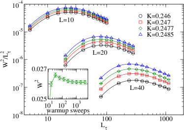
Figure 1: Selection of Monte Carlo results for the winding number fluctuation divided by $L_{\tau}^{2}$ as a function of $L_{\tau}$. Solid curves are polynomial fits to the data curves, from which the locations $L_{\tau}^{*}$ and sizes $(W^{2}/L_{\tau}^{2})^{*}$ of the maxima can be determined. Inset: Equilibration test for $L=40,L_{\tau}=240,K=0.2477$.

Results – First we locate the critical coupling $K_{\text{c}}$ and the dynamic exponent $z$ by FSS analysis of MC data for the winding number. Figure 1 shows examples of maxima of the quantity $W^{2}/L_{\tau}^{2}$. The amplitude $(W^{2}/L_{\tau}^{2})^{*}$ and location $L_{\tau}^{*}$ of the maxima can be straightforwardly computed by polynomial fits to the MC data curves. Better accuracy is obtained in the estimates for $(W^{2}/L_{\tau}^{2})^{*}$ than for $L_{\tau}^{*}$. The maximum values scale as $(W^{2}/L_{\tau}^{2})^{*}\sim L^{-2z}$ at $K=K_{c}$. However it is more convenient to plot the quantity $\Phi^{*}=(W^{2}/\alpha_{\tau}^{2})^{*}$ of Eq. (5), and look for the scaling $\Phi^{*}\sim L^{0}$ at $K=K_{c}$, which is shown in a log-log plot in Fig. 2. In the figure the of value $z$ enters through $\alpha_{\tau}^{*}=L_{\tau}^{*}/L^{z}$, and has been adjusted to make $\Phi^{*}=const$ at $K=K_{c}$ for system sizes $L>16$, marked with the horizontal dashed line. This produces the estimates $z\approx 1.8$ and $K_{c}\approx 0.2477$. For $K\neq K_{\text{c}}$ the data curves clearly splay out, away from a critical power law. For $L<16$ deviation from power law behavior is obtained, which indicates the presence of corrections to scaling in these data points. In Fig. 2 we also note that the choice $z=2$ gives an approximate description of the data for $K=0.246$ for small system sizes, $L<16$, which is indicated by the lower dashed line, in agreement with Ref. Alet:2003p741 . As a consistency test, a similar analysis was done for the location $L_{\tau}^{*}$ of the maxima using the relation $L_{\tau}^{*}\sim L^{z}$ at $K=K_{c}$, leading to similar results.

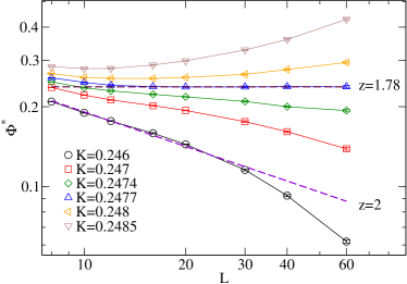
Figure 2: Maximum values $\Phi^{*}=(W^{2}/\alpha_{\tau}^{2})^{*}$ vs. system size $L$ for different couplings $K$. For $z=1.78$ the data obeys $\Phi^{*}=const$ at $K=K_{c}$ for $L\geq 16$, indicated by the horizontal dashed line, which estimates $K_{c}=0.2477$. The lower dashed line corresponds to $z=2$, which approximately describes the data for small sizes $L<16$ at $K=0.246$.

Figure 3 A shows the maxima of the function $\Phi^{*}$ of Eq. (5), with $\alpha=L_{\tau}/L^{z}$ for $z\approx 1.8$. The data curves for $L>16$ intersect at $K_{c}$, but for smaller sizes scaling deviations are present, and these will be further discussed below. The correlation length exponent is readily estimated by computing the derivatives $\partial\Phi^{*}/\partial K|_{K=K_{c}}\sim L^{1/\nu}$, and a polynomial fit to the MC data gives $\nu\approx 1.15$. The FSS data collapse produced by using this value for $\nu$ is shown in Fig. 3 B for $L>16$.

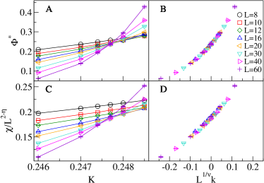
Figure 3: A: Intersection plot for the scaled winding number function maxima $\Phi^{*}$, showing an intersection at $K_{c}=0.2477$. B: FSS data collapse of the data in A obtained for $\nu=1.15,L\geq 16$. C: Intersection plot for the scaled susceptibility $\chi/L^{2-\eta}$ evaluated at $\alpha_{\tau}=0.35$. The data curves for large sizes roughly intersect at $K=0.2477$ for $\eta=-0.29$, but with much larger corrections visible for small system sizes than for $\Phi^{*}$. D: FSS data collapse of $\chi/L^{2-\eta}$ for $\nu=1.15,L\geq 16$.

To estimate the correlation function exponent $\eta$ we use the susceptibility $\chi$ given by Eq. (4). We fix the aspect ratio to $\alpha_{\tau}=0.35$ which correspond to the maxima $\Phi^{*}$ at criticality. The value of $\chi$ at this aspect ratio was determined by a polynomial fit to nearby MC data. From $\chi\sim L^{2-\eta}$ we estimate $\eta\approx-0.3$ for $L\geq 16$. Figure 3 C shows a corresponding intersection plot for the quantity $\chi/L^{2-\eta}$, which becomes size independent at $K=K_{c}$ according to Eq. (4). A FSS collapse assuming $\nu=1.15$ is shown in Fig. 3 D. Note that the deviations from scaling for small system sizes in Fig. 3 C are substantial, and hence the uncertainty in the estimate of $\eta$ is considerable. The scatter among the intersection points can be reduced by assuming a scaling correction proportional to $L^{-\omega}$ with $\omega\approx 1$, but the accuracy of the data is insufficient for detailed estimates.

Finally we systematically study the system size dependence of the estimated exponents and estimate errors. This final calculation does not involve the maxima, and thus avoids any errors in their determination. A double polynomial expansion is done of the scaling functions in Eq. (5) in both arguments. The parameters are determined by $\chi^{2}$-minimization of the RMS deviations of the MC data points from the scaling function. We performed several fits for MC data points selected from different intervals in the range $0.2<\alpha_{\tau}<1.2$ in order to verify the stability of the results. To study system size trends of the results, fits were made for a sequence of system size quadruplets in $L=8,10,12,16,20,30,40,60$. The result for $z$ is shown in the inset of Fig. 4. The displayed trend agrees with the one indicated in Fig. 2. For the fit with $L=16,20,30,40$, $0.2<\alpha_{\tau}<0.5$, we get $\chi^{2}/{\rm DOF}\approx 0.8$. Our final estimates including error estimates based on statistical errors determined by the bootstrap method combined with average variations from the dependence on the $\alpha_{\tau}$-interval included in the fits are $K_{c}=0.2477\pm 0.0002,z=1.8\pm 0.05,\nu=1.15\pm 0.03$, and $\eta=-0.3\pm 0.1$. Other critical exponents can be estimated from these values using scaling laws.

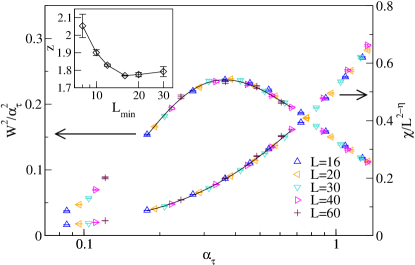
Figure 4: FSS data collapses of MC data for the scaled winding number fluctuation $\Phi=W^{2}/\alpha_{\tau}^{2}$ and susceptibility $\chi/L^{2-\eta}$ as functions of $\alpha_{\tau}=L_{\tau}/L^{z}$ for $K_{\text{c}}=0.2477,z=1.8,\eta=-0.29$. Solid curves are polynomial fits to the data. Inset: Dependence of $z$ on the range of system sizes used in the estimate. $L_{\rm min}$ indicates the smallest in a sequence of size quadruplets in $L=8,10,12,16,20,30,40,60$ used to estimate $z$, except for $L_{\rm min}=30$ which indicates sizes $30,40,60$.

Discussion – Analysis of our MC data of the 2D boson localization transition by disorder revises previous estimates of the critical exponents. In particular the dynamic critical exponent is estimated to $z=1.8\pm 0.05$, which suggests that $z=d$ is not fulfilled in $d=2$, although the values are close. Our results clarify how most previous simulations appear consistent with $z=2$. For small system sizes $z=2$ works quite well, but including larger sizes reveals corrections to scaling making $z=1.8$ a better estimate. Our estimates are quite different from those of Ref. Priyadarshee:2006p740 , which we believe may be explained by their smaller disorder averaging and uncertainty in their location of the quantum critical point. The prediction of a universal conductivity at the transition is independent of the value of $z$ Fisher:1989p868 . However, actual estimates of the universal value of the conductivity indirectly depend on the value of $z$, and should be reexamined in the light of the present results. A better analytic understanding of the quantum critical dynamics as well as further experimental measurements probing these issues would be welcome.

We acknowledge valuable discussions with Steve Girvin, Steve Teitel, and Igor Herbut. This project was supported by the Swedish Research Council and by the Swedish National Infrastructure for Computing via PDC.

References

- (1) S. Sondhi, S. Girvin, J. Carini, and D. Shahar, Rev. Mod. Phys. 69, 315 (1997)
- (2) S. Sachdev, Quantum Phase Transitions (Cambridge University Press, UK, 1999)
- (3) M. P. A. Fisher, P. B. Weichman, G. Grinstein, and D. S. Fisher, Phys. Rev. B 40, 546 (1989)
- (4) M. White, M. Pasienski, D. McKay, S. Q. Zhou, D. Ceperley, and B. DeMarco, Phys. Rev. Lett. 102, 055301 (2009)
- (5) P. B. Weichman and R. Mukhopadhyay, Phys. Rev. Lett. 98, 245701 (2007)
- (6) P. B. Weichman and R. Mukhopadhyay, Phys. Rev. B 77, 214516 (2008)
- (7) A. Priyadarshee, S. Chandrasekharan, J.-W. Lee, and H. U. Baranger, Phys. Rev. Lett. 97, 115703 (2006)
- (8) E. S. Sørensen, M. Wallin, S. M. Girvin, and A. P. Young, Phys. Rev. Lett. 69, 828 (1992)
- (9) M. Wallin, E. S. Sørensen, S. M. Girvin, and A. P. Young, Phys. Rev. B 49, 12115 (1994)
- (10) F. Alet and E. S. Sørensen, Phys. Rev. E 67, 015701 (2003)
- (11) F. Lin, E. S. Sørensen, and D. M. Ceperley, Phys. Rev. B 84, 094507 (2011)
- (12) I. F. Herbut, Phys. Rev. B 61, 14723 (2000)
- (13) N. Prokof’ev and B. Svistunov, Phys. Rev. Lett. 87, 160601 (2001)
- (14) E. L. Pollock and D. M. Ceperley, Phys. Rev. B 36, 8343 (1987)
- (15) A. Vestergren, M. Wallin, S. Teitel, and H. Weber, Phys. Rev. B 70, 054508 (2004)