A comparative study of the electronic and magnetic properties of BaFe₂As₂ and BaMn₂As₂ using the Gutzwiller approximation

Abstract

To elucidate the role played by the transition metal ion in the pnictide materials, we compare the electronic and magnetic properties of BaFe₂As₂ with BaMn₂As₂. To this end we employ the LDA+Gutzwiller method to analyze the mass renormalizations and the size of the ordered magnetic moment of the two systems. We study a model that contains all five transition metal 3d orbitals together with the Ba-5d and As-4p states (ddp-model) and compare these results with a downfolded model that consists of Fe/Mn d-states only (d-model). Electronic correlations are treated using the multiband Gutzwiller approximation. The paramagnetic phase has also been investigated using LDA+Gutzwiller method with electron density self-consistency. The renormalization factors for the correlated Mn 3d orbitals in the paramagnetic phase of BaMn₂As₂ are shown to be generally smaller than those of BaFe₂As₂, which indicates that BaMn₂As₂ has stronger electron correlation effect than BaFe₂As₂. The screening effect of the main As 4p electrons to the correlated Fe/Mn 3d electrons is evident by the systematic shift of the results to larger Hund’s rule coupling J side from the ddp-model compared with those from the d-model. A gradual transition from paramagnetic state to the antiferromagnetic ground state with increasing $J$ is obtained for the models of BaFe₂As₂ which has a small experimental magnetic moment; while a rather sharp jump occurs for the models of BaMn₂As₂, which has a large experimental magnetic moment. The key difference between the two systems is shown to be the d-level occupation. BaMn₂As₂, with approximately five d-electrons per Mn atom, is for same values of the electron correlations closer to the transition to a Mott insulating state than BaFe₂As₂. Here an orbitally selective Mott transition, required for a system with close to six electrons only occurs at significantly larger values for the Coulomb interactions.

I Introduction

The discovery of high T_c superconductivity in LaO_1-xF_xFeAs has initiated a detailed investigation of these and related iron based compounds with the ultimate aim to identify new high temperature superconductorsKamihara08 . Many binary, ternary and quaternary compounds have been synthesized and investigated experimentally, some of which were quickly found to exhibit high T_c superconductivity with electron or hole doping or under pressure or intrinsically Rotter08 ; Wu08 ; Tapp08 ; Torika08 ; Chen08 ; Ren08 . Meanwhile, several closely related and physically interesting systems have also been studied. An interesting example is the BaMn₂As₂ compound, which has the same layered tetragonal ThCr₂Si₂-type crystal structure as the BaFe₂As₂ at room temperatureSingh09 ; Singh091 ; An09 ; Johnston10 . BaMn₂As₂ is an antiferromagnetic (AFM) insulator with a small gap; while BaFe₂As₂, a parent compound of the Fe-based high T_c superconductors, is an AFM metal at low temperatures. The more localized behavior of the ordered magnetic state in the Mn-based system suggests that electronic correlations in this system are stronger or more efficient in changing the electronic properties of the material. A closer, comparative investigation of distinct transition metal ions therefore promises to reveal further whether iron is indeed special among its neighbors in the periodic table. This is also expected on qualitative grounds on the basis of the Hund’s rule pictureHaule09 .

Theoretically, the description of the normal states for iron pnictide superconductors is complicated by the multi-orbital nature and the presence of electron correlation effects. Interesting results can be obtained from low energy theories that are primarily concerned with states in the immediate vicinity of the Fermi surfaceKuroki08 ; Raghu08 ; Chubukov08 ; Cvetkovic09 ; Zhai09 ; Sknepnek09 . However, material specific insight often requires a careful analysis of states over a larger energy window. In the iron pinctide and chalcogenides the strength of the correlations is controlled by the Hund’s rule coupling $J$, rather than by the Hubbard $U$ or the p-d charge transfer energyHaule09 . This makes these materials a new class of correlated metals, different from doped Mott or charge transfer insulators. Calculations based on density functional theory (DFT) usually yield too wide Fe 3d bands and too large magnetic moment in the AFM ground stateMazin08 . Recently the AFM phase of the iron pnictide parent compounds has been successfully described by using a combination of DFT and dynamical mean field theory (DMFT) with full charge self-consistencyYin11 . These investigations clearly demonstrated the important role played by the Hund’s rule coupling $J$ for the magnetic and electronic properties of the iron pnictides. A systematic analysis of a large class of Fe-based materials further demonstrated that the nature and strength of local correlations are rather universal, while material specifics result from changes in the kinetic energy, amplified by the frustrated nature of electron hopping path due to Fe-As-Fe and direct Fe-Fe overlapsYin11b . This universality in the value of the local Coulomb interactions $U$, $U^{\prime}$, $J$ only exists if one includes in addition to the Fe-3d states at least the As 4p orbitals. Downfolding to models with iron states only is sufficient to lead to material specific variations in the local correlations. In view of these insights is it important to compare the behavior of Fe-based systems with systems based on other transition metals, also in view of the ongoing debate whether these systems should be considered weakly or strongly correlated.

On a technical level, quite a few efforts have been devoted to study the electronic and magnetic properties of the systems using the Gutzwiller variational methodDai10 and simplified tight-binding modelszhou10 ; Bune11 with the particular appeal that the Gutzwiller approach is computationally cheaper if compared to more sophisticated DMFT approaches such as the usage of Quantum Monte Carlo algorithms. For example. the experimental magnetic moment was obtained in a three band Hubbard model of LaOFeAs which contains only Fe 3d $t_{2g}$ orbitalszhou10 . Calculations based on the five-band model show that the $e_{g}$ orbitals are also important and the system exhibits a sharp transition from paramagnetic (PM) state to AFM state with large magnetic moment when $J$ increases, which is different from the results of three-band modelBune11 . Another important question is whether, in addition to the Fe 3d $e_{g}$ orbitals, the inclusion of As 4p elections is required for a more quantitative description of the AFM and paramagnetic phases. Finally, recent calculations for LaOFeAs  based on the LDA+Gutzwiller approach that includes a Fe3d–As4p Wannier-orbital basis does indeed reproduce the experimentally observed small ordered magnetic moment over a large region of ($U,J$) parameter spaceWeber .

In this paper, we report a comparative study of the BaFe₂As₂ and BaMn₂As₂ on the electronic and magnetic properties by investigating the Fe/Mn d-band model and the ddp-model that includes Fe/Mn 3d, Ba 5d, and As 4p orbitals with Gutzwiller approximationGutzwiller1 ; Gutzwiller2 ; Bunemann07 which has been shown to be equivalent to a slave-boson mean field theoryKotliar86 . The paramagnetic phase for the two systems has also been investigated using LDA+Gutzwiller method with electron density self-consistencyDai08 ; Dai09 . BaMn₂As₂ is shown to be a more correlated material than BaFe₂As₂. The screening effect of the As 4p electrons is evident by the comparison between the results of the Fe/Mn d-model and those of the ddp-model or LDA+Gutzwiller method. The key difference in the behavior of these systems is shown to be the distinct electron count of the 3d states, a result that is robust against changes in the detailed description of these systems. While the even number of electrons for an Fe site requires that the system undergoes an orbitally selective Mott transition, Mn with five electrons can more easily localize and therefore has a much stronger tendency towards large moment magnetism and Mott localization, even for the nominally same values of the Coulomb interactions. The prospect to tune the tendency towards localization by varying the transition metal ions may therefore play an important role in optimizing the strength of electronic correlations for high temperature superconductivity.

II Formalism

For the sake of being self-contained, we outline the main formalisms for the multiband model with the Gutzwiller approximationGutzwiller1 ; Gutzwiller2 ; Bunemann07 and the LDA+Gutzwiller approach with electron density self-consistencyDai08 ; Dai09 .

II.1 Multiband model with the Gutzwiller approximation

The multi-band Hamiltonian with local many-body interactions is written as

$$\mathcal{H}=\mathcal{H}_{0}+\mathcal{H}_{1}$$ (1)

where the bare paramagnetic band Hamiltonian ($\mathcal{H}_{0}$) is

$$\mathcal{H}_{0}=\sum_{\left(i\alpha\right)\neq\left(j\beta\right),\sigma}t_{i\alpha j\beta}c_{i\alpha\sigma}^{\dagger}c_{j\beta\sigma}+\sum_{i,\alpha,\sigma}\varepsilon_{i\alpha}c_{i\alpha\sigma}^{\dagger}c_{i\alpha\sigma}$$ (2)

$t_{i\alpha j\beta}$ is the electron hopping element between orbital $\varphi_{\alpha}$ at site $i$ and orbital $\varphi_{\beta}$ at site $j$. $\varepsilon_{i\alpha}$ is the orbital level.  For the Fe/Mn d-model, $\alpha$ and $\beta$ run over the Fe/Mn 3d orbitals. For the ddp-model, $\alpha$ and $\beta$ run over the Fe/Mn 3d orbitals, Ba 5d orbitals, and As 4p orbitals. $c^{\dagger}$($c$) is the electron creation (annihilation) operator. $\sigma$ is the spin index.

The typical Hubbard density-density type interaction term ($\mathcal{H}_{1}$) for Fe 3d electrons is

$$\mathcal{H}_{1} =U\sum_{i,\gamma}n_{i\gamma\uparrow}n_{i\gamma\downarrow}+U^{\prime}\sum_{i,\gamma<\gamma^{\prime},\sigma\sigma^{\prime}}n_{i\gamma\sigma}n_{i\gamma^{\prime}\sigma^{\prime}}$$

$$-J\sum_{i,\gamma<\gamma^{\prime},\sigma}n_{i\gamma\sigma}n_{i\gamma^{\prime}\sigma}$$ (3)

which is usually sufficient for describing collinear magnetic orderzhou10 . Here $\gamma$ is the correlated Fe/Mn 3d orbital index, $U^{\prime}=U-2J$, and $n_{i\gamma\sigma}=c_{i\gamma\sigma}^{\dagger}c_{i\gamma\sigma}$.

We take a variational wave function of the Gutzwiller form,

$$\left|\Psi_{G}\right\rangle=\frac{\hat{G}\left|\Psi_{0}\right\rangle}{\sqrt{\left\langle\Psi_{0}\left|\hat{G}^{2}\right|\Psi_{0}\right\rangle}}$$ (4)

with the Gutzwiller approximation to calculate the expectation values of Eq. 1 Gutzwiller1 ; Gutzwiller2 ; Bunemann07 . $\Psi_{0}$ is the uncorrelated wave function. $\hat{G}$ is the Gutzwiller projection operator, which adopts the following form

$$\hat{G}=e^{-\sum_{i\mathcal{F}}g_{i\mathcal{F}}\left|\mathcal{F}_{i}\right\rangle\left\langle\mathcal{F}_{i}\right|}$$ (5)

where $\left|\mathcal{F}_{i}\right\rangle$ is the Fock state generated by a set of $\left\{c_{i\gamma\sigma}^{\dagger}\right\}$

$$\left|\mathcal{F}_{i}\right\rangle={\displaystyle\prod\limits_{\gamma\sigma}}\left(c_{i\gamma\sigma}^{\dagger}\right)^{n_{i\gamma\sigma}^{\mathcal{F}}}\left|0\right\rangle$$ (6)

with $n_{i\gamma\sigma}^{\mathcal{F}}=0$ or $1$, which identifies whether there is an electron with spin $\sigma$ occupied in orbital $\gamma$ for Fock state $\mathcal{F}$ at the $i^{th}$ site. $g_{i\mathcal{F}}$ is a variational parameter which controls the weight of the local Fock state $\left|\mathcal{F}_{i}\right\rangle$ in the Gutzwiller wave function. $g_{i\mathcal{F}}=1$ for the empty and singly occupied configurations because in these cases there are no electron-electron repulsion involved. According to Ref. Bunemann07 , the expectation value of the electron Hamiltonian $\mathcal{H}$ can be expressed as

$$\left\langle\mathcal{H}\right\rangle_{G} =\sum_{i\alpha,j\beta,\sigma}\left(z_{i\alpha\sigma}z_{j\beta\sigma}t_{i\alpha j\beta}+\varepsilon_{i\alpha}\delta_{\alpha\beta}\delta_{ij}\right)\left\langle c_{i\alpha\sigma}^{\dagger}c_{j\beta\sigma}\right\rangle_{0}$$

$$+\sum_{i\mathcal{F}}U_{i\mathcal{F}}p_{i\mathcal{F}}$$ (7)

where $\left\langle c_{i\alpha\sigma}^{\dagger}c_{j\beta\sigma}\right\rangle_{0}=\left\langle\Psi_{0}\left|c_{i\alpha\sigma}^{\dagger}c_{j\beta\sigma}\right|\Psi_{0}\right\rangle$ and $U_{i\mathcal{F}}=\left\langle\mathcal{F}_{i}\left|\mathcal{H}_{1}\right|\mathcal{F}_{i}\right\rangle$. We define the Gutzwiller orbital renormalization factor $z_{i\alpha\sigma}\equiv 1$ for Ba 5d and As 4p orbitals in the ddp-model since they are not considered as strongly correlated orbitals. Following Ref. Bunemann07 , for the Fe/Mn 3d orbitals

$$z_{i\gamma\sigma}=\frac{1}{\sqrt{n_{i\gamma\sigma}^{0}\left(1-n_{i\gamma\sigma}^{0}\right)}}\sum_{\mathcal{F},\mathcal{F}^{\prime}}\sqrt{p_{i\mathcal{F}}p_{i\mathcal{F}^{\prime}}}\left|\left\langle\mathcal{F}_{i}\left|c_{i\gamma\sigma}^{\dagger}\right|\mathcal{F}_{i}^{\prime}\right\rangle\right|^{2}$$ (8)

with $n_{i\gamma\sigma}^{0}=\left\langle n_{i\gamma\sigma}\right\rangle_{0}$. $p_{i\mathcal{F}}$ is the occupation probability of configuration $\left|\mathcal{F}_{i}\right\rangle$, which absorbs $g_{i\mathcal{F}}$ and serves as the additional variational parameter due to the Gutzwiller wave function.

Since $\mathcal{H}_{0}$ in the Hamiltonian of Eq. 1 is obtained by downfolding the DFT band structure, some contributions from $\mathcal{H}_{1}$ have already been taken into account by $\mathcal{H}_{0}$ in a mean-field way. Such contributions are commonly referred to as the double counting term. Consequently, the total energy of the system is given by

$$E_{tot}=\left\langle\mathcal{H}\right\rangle_{G}+E_{d.c.}$$ (9)

with

$$E_{d.c.}=-\sum_{i}\left(\bar{U}N_{id}\left(N_{id}-1\right)/2-\bar{J}N_{id}\left(N_{id}/2-1\right)/2\right)$$ (10)

following the treatment in DFT+U methodDC1 ; DC2 . Here $\bar{U}$ ($\bar{J}$) is the averaged Coulomb U (Hund’s rule coupling J) parameter, which for d orbitals is given asDai09 ; Kotliar06

$$\bar{U}=\frac{U+4U^{\prime}}{5}$$ (11)

$$\bar{J}=\bar{U}-U^{\prime}+J$$ (12)

$N_{id}=\sum_{\gamma\sigma}n_{i\gamma\sigma}^{0}$ is the expectation value of the total Fe/Mn d-orbital occupancy at site $i$. The double counting term $E_{d.c.}$ introduces some spin-independent chemical potential shift for the Fe/Mn 3d orbitals,

$$\mathcal{\tilde{\varepsilon}}_{i\gamma}=-\bar{U}\left(N_{id}-\frac{1}{2}\right)+\bar{J}\left(N_{id}/2-\frac{1}{2}\right)$$ (13)

In the Fe/Mn d-model that contains only 3d states, $\mathcal{\tilde{\varepsilon}}_{i\gamma}$ has no effect since it merely shifts all the Fe/Mn 3d levels by a constant. However, in the ddp-models $\mathcal{\tilde{\varepsilon}}_{i\gamma}$ becomes important because it changes the position of the Fe/Mn 3d levels with respect to Ba 4d and As 4p orbitals and hence affects the electron flow between these orbitals.

The minimization of $E_{tot}$ with the constraints of $\sum_{\mathcal{F}}p_{i\mathcal{F}}=1$ and $\sum_{\mathcal{F}}p_{i\mathcal{F}}n_{i\gamma\sigma}^{\mathcal{F}}=n_{i\gamma\sigma}^{0}$ yields an effective single-particle Hamiltonian

$$H_{\text{eff}}=\sum_{i\alpha,j\beta,\sigma}\left(z_{i\alpha\sigma}z_{j\beta\sigma}t_{i\alpha j\beta}+\mu_{i\alpha\sigma}\delta_{\alpha\beta}\delta_{ij}\right)c_{i\alpha\sigma}^{\dagger}c_{j\beta\sigma}$$ (14)

where $\mu_{i\alpha\sigma}=\varepsilon_{i\alpha}+\mathcal{\tilde{\varepsilon}}_{i\alpha}+\frac{\partial z_{i\alpha\sigma}}{\partial n_{i\alpha\sigma}^{0}}e_{i\alpha\sigma}+\eta_{i\alpha\sigma}$ if $\alpha$ belongs to the correlated Fe/Mn 3d orbitals and $\mu_{i\alpha\sigma}=\varepsilon_{i\alpha}$ otherwise. It has been shown that $H_{\text{eff}}$ describes the Landau-Gutzwiller quasiparticle bandsBunemann03 , and the square of the orbital renormalization factor $z^{2}$ corresponds to the quasiparticle weightDai09 . $\left\{z_{i\gamma\sigma}\right\}$ and $\left\{\eta_{i\gamma\sigma}\right\}$ are obtained by solving the following equations.

$$\sum_{\mathcal{F}^{\prime}}\mathcal{M}_{\mathcal{FF}^{\prime}}^{i}\sqrt{p_{i\mathcal{F}^{\prime}}}=\eta_{i0}\sqrt{p_{i\mathcal{F}}}$$ (15)

where

$$\mathcal{M}_{\mathcal{F},\mathcal{F}^{\prime}}^{i}=\sum_{\gamma\sigma}\frac{e_{i\gamma\sigma}}{2\sqrt{n_{i\gamma\sigma}^{0}\left(1-n_{i\gamma\sigma}^{0}\right)}}\left|\left\langle\mathcal{F}_{i}\left|c_{i\gamma\sigma}^{\dagger}+c_{i\gamma\sigma}\right|\mathcal{F}_{i}^{\prime}\right\rangle\right|^{2}+\delta_{\mathcal{FF}^{\prime}}\left(U_{i\mathcal{F}}-\sum_{\gamma\sigma}\eta_{i\gamma\sigma}n_{i\gamma\sigma}^{\mathcal{F}}\right)$$ (16)

with $e_{i\gamma\sigma}=\sum_{j\beta}\left(z_{j\beta\sigma}t_{i\alpha j\beta}\left\langle c_{i\gamma\sigma}^{\dagger}c_{j\beta\sigma}\right\rangle_{0}+c.c.\right)$. $\Psi_{0}$ from Eq. 14 and $\left\{p_{i\mathcal{F}}\right\}$ from Eq. 15 need to be solved self-consistently to obtain the final solutionYYX11 .

II.2 LDA+Gutzwiller

The

above formalism based on the Gutzwiller approximation on the multiband model can be naturally combined with DFT, in which full electron density convergence can be achievedDai08 ; Dai09 ; Ho08 . The total energy density functional can be written as

$$E\left[\rho\right]=\left\langle\Psi_{G}\left|\hat{T}\right|\Psi_{G}\right\rangle+E_{H}\left[\rho\right]+E_{xc}+\int\rho\left(\mathbf{r}\right)v_{ion}\left(\mathbf{r}\right)d^{3}r+E_{ion-ion}$$ (17)

where $\hat{T}$ is the kinetic energy operator and $E_{H}$ is the Hartree potential energy. The electron-ion and ion-ion potential energies are given by $\int\rho\left(\mathbf{r}\right)v_{ion}\left(\mathbf{r}\right)d^{3}r$ and $E_{ion-ion}$, respectively. In the LDA+Gutzwiller methodDai08 ; Dai09 , the approximate exchange-correlation energy $E_{xc}$ takes the following form

$$E_{xc}=E_{xc}^{LDA}\left[\rho\right]+\sum_{i\mathcal{F}}U_{i\mathcal{F}}p_{i\mathcal{F}}+E_{d.c.}$$ (18)

The electron density $\rho$ under the Gutzwiller approximation can be written as

$$\rho\left(\mathbf{r}\right)=\sum_{i\alpha,j\beta,\sigma}^{\prime}z_{i\alpha\sigma}z_{j\beta\sigma}\varphi_{i\alpha}^{\ast}\left(\mathbf{r}\right)\varphi_{j\beta}\left(\mathbf{r}\right)\left\langle c_{i\alpha\sigma}^{\dagger}c_{j\beta\sigma}\right\rangle_{0}+\sum_{i\alpha,\sigma}\left|\varphi_{i\alpha}\left(\mathbf{r}\right)\right|^{2}\left\langle n_{i\alpha\sigma}\right\rangle_{0}$$ (19)

where $\left\{\varphi_{i\alpha}\right\}$ is a general complete basis set including local correlated orbitals (e.g., Fe/Mn 3d orbitals) as well as nonlocal orbitals. $\sum^{\prime}$ indicates that the summation excludes the term with $i\alpha=j\beta$. The kinetic energy is also renormalized

$$\left\langle\Psi_{G}\left|\hat{T}\right|\Psi_{G}\right\rangle=\sum_{i\alpha,j\beta,\sigma}^{\prime}z_{i\alpha\sigma}z_{j\beta\sigma}\left\langle\varphi_{i\alpha}\left|\hat{T}\right|\varphi_{j\beta}\right\rangle\left\langle c_{i\alpha\sigma}^{\dagger}c_{j\beta\sigma}\right\rangle_{0}+\sum_{i\alpha,\sigma}\left\langle\varphi_{i\alpha}\left|\hat{T}\right|\varphi_{i\alpha}\right\rangle\left\langle n_{i\alpha\sigma}\right\rangle_{0}$$ (20)

The total energy $E\left[\rho\right]$ of the closed form can be similarly minimized as in the above multiband model with respect to $\Psi_{0}$ and $\left\{p_{i\mathcal{F}}\right\}$. The resultant effective single-particle Hamiltonian has the same form as Eq. 14 with the hopping element

$$t_{i\alpha j\beta}=\left\langle\varphi_{i\alpha}\left|\hat{T}\right|\varphi_{j\beta}\right\rangle+\int\left(v_{scr}^{LDA}\left(\mathbf{r}\right)+v_{ion}\left(\mathbf{r}\right)\right)\varphi_{i\alpha}^{\ast}\left(\mathbf{r}\right)\varphi_{j\beta}\left(\mathbf{r}\right)d^{3}r$$ (21)

The LDA screening potential $v_{scr}^{LDA}\left(\mathbf{r}\right)$ is the sum of the Hartree potential $v_{H}\left(\mathbf{r}\right)=\frac{\delta E_{H}\left[\rho\right]}{\delta\rho}$ and the exchange-correlation potential $v_{xc}^{LDA}\left(\mathbf{r}\right)=\frac{\delta E_{xc}^{LDA}\left[\rho\right]}{\delta\rho}$. The renormalized orbital level $\mu_{i\alpha\sigma}=\varepsilon_{i\alpha}+\tilde{\varepsilon}_{i\alpha}+\frac{\partial z_{i\alpha\sigma}}{\partial n_{i\alpha\sigma}^{0}}\tilde{e}_{i\alpha\sigma}+\eta_{i\alpha\sigma}$ if $\alpha$ belongs to the correlated Fe/Mn 3d orbitals and $\mu_{i\alpha\sigma}=\varepsilon_{i\alpha}$ otherwise. Here $\varepsilon_{i\alpha}=t_{i\alpha i\alpha}$ and $e_{i\gamma\sigma}=\sum_{j\beta}\left(z_{j\beta\sigma}t_{i\alpha j\beta}\left\langle c_{i\gamma\sigma}^{\dagger}c_{j\beta\sigma}\right\rangle_{0}+c.c.\right).\left\{z_{i\gamma\sigma}\right\}$ and $\left\{\eta_{i\gamma\sigma}\right\}$ are obtained by solving the same equation as Eq.15. One can see that the major difference is that the hopping element $t_{i\alpha j\beta}$ and the orbital level $\varepsilon_{i\alpha}$ will be updated self-consistently by the LDA screening potential $v_{scr}^{LDA}\left(\mathbf{r}\right)$ in LDA+Gutzwiller method, while they are fixed in the multiband model.

III Effects caused by downfolding

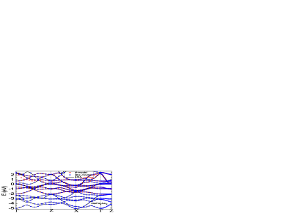
Figure 1: (Color online) Band structure of BaFe₂As₂ in PM phase based on LDA (solid line), Fe d-model (circle) and ddp-model calculations (cross). Fermi level is shifted to zero.

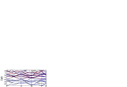
Figure 2: (Color online) Band structure of BaMn₂As₂ with settings same as Fig. 1.

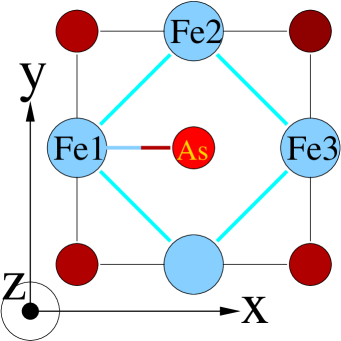
Figure 3: (Color online) The atomic configuration of the Fe-As layer with the coordinate system. Note that the center As atom is above the Fe-plane, while the corner As atoms are below the Fe-plane.

Fe1/Mn1	$xy$	$yz$	$z^{2}$	$xz$	$x^{2}-y^{2}$
Fe2/Mn2: $xy$	-0.34/-0.32 (-0.35/-0.33)	0.25/0.20 (0.21/0.17)	0.31/0.28 (0.27/0.24)	-0.25/-0.20 (-0.21/-0.17)	0
$yz$	0.25/0.20 (0.21/0.17)	-0.22/-0.16 (-0.14/-0.10)	-0.11/-0.10 (-0.09/-0.08)	0.12/0.11 (0.08/0.08)	0.18/0.16 (0.17/0.15)
$z^{2}$	0.31/0.28 (0.27/0.24)	-0.11/-0.10 (-0.09/-0.08)	0.06/0.03 (0.01/-0.01)	0.11/0.10 (0.09/0.08)	0
$xz$	-0.25/-0.20 (-0.21/-0.17)	0.12/0.11 (0.08/ 0.08)	0.11/0.10 (0.09/0.08)	-0.22/-0.16 (-0.14/-0.10)	0.18/0.16 (0.17/0.14)
$x^{2}-y^{2}$	0	0.18/0.16 (0.17/0.15)	0	0.18/0.16 (0.17/0.15)	-0.13/-0.07 (-0.09/-0.03)
Fe3/Mn3: $xy$	-0.07/-0.05 (-0.06/-0.05)	0.14/0.11 (0.10/0.08)	0	0	0
$yz$	-0.14/-0.11 (-0.10/-0.08)	0.15/0.11 (0.08/0.07)	0	0	0
$z^{2}$	0	0	-0.01/-0.02 (0/-0.01)	0.17/0.15 (0.13/0.12)	-0.18/-0.13 (-0.12/-0.08)
$xz$	0	0	-0.16/-0.15 (-0.13/-0.12)	0.32/0.27 (0.20/0.17)	0.04/0.06 (0.04/0.05)
$x^{2}-y^{2}$	0	0	-0.17/-0.13 (-0.12/-0.08)	-0.04/-0.06 (-0.04/-0.05)	0.11/0.09 (0.09/0.07)
As: $y$	(-0.50/-0.42)	(0.39/0.33)	0	0	0
$z$	0	0	(0.34/0.29)	(0.09/0.12)	(-0.49/-0.41)
$x$	0	0	(0.14/0.13)	(-0.69/-0.58)	(0.32/0.25)

Table 1: The hopping parameters between the orbitals of Fe1/Mn1 and those of its nearest neighbour Fe2/Mn2, next nearest neighbour Fe3/Mn3 and the center As atom. The entries of A1/B1(A2/B2) mean that A1 is the hopping parameter in the Fe d-model and B1 in the Mn d-model. A2 and B2 are the corresponding values in the ddp-models.

The Fe/Mn d-model and ddp-model for BaFe₂As₂ and BaMn₂As₂ have been obtained by downfolding the first-principles LDA electron bands of the experimentally determined crystal structuresRotter081 ; Singh091 using the quasi-atomic minimal basis-set orbitals (QUAMBOs)QUAMBO1 ; QUAMBO2 ; QUAMBO3 ; QUAMBO4 . The main idea of the QUAMBO approach is to recover a set of local quasi-atomic orbitals by performing an inverse unitary transformation for the “bonding” and “anti-bonding” states. In practice, the “bonding states” are some occupied bands or low energy bands which are intended to be preserved in the new local orbital representation. The “anti-bonding” states are constructed from the orthogonal subspace of the “bonding” subspace and are optimized such that resultant QUAMBOs have maximal similarity with the free atomic orbitals. The orthogonal subspace is spanned by the wave functions in some energy window. It becomes complete in the infinite energy or band limit, where succinct closed form for QUAMBOs can still be obtainedQUAMBO3 . In principle, different choices of the “bonding”  states and the energy window for the “anti-bonding” states will yield different set of QUAMBOs and tight-binding parameters, which is reasonable and acceptable since the downfolding of the band structure should not be unique. We find that the ddp model will give too many Fe/Mn d-electrons if it is obtained by treating all the occupied states and virtual states up to $2$eV above Fermi level as the “bonding” states in the infinite band limit: $7.3$ d-electrons per Fe atom for BaFe₂As₂ (close to the analysis of Ref.Ciraci09 ) and $6.2$ for BaMn₂As₂, while the nominal value would be $6$ and $5$, respectively. Such large deviation of the correlated electron number clearly do not properly reflect the correct physics of these materials. This problem does not exist for the Fe/Mn d-model where the electron filling is fixed by assumption. In order to have a general tight-binding model suitable for the correlated local orbital-based approaches, we choose a finite energy window around the Fermi level for the generation of the “anti-bonding” states and another smaller energy window to control the Bloch bands which will contribute to the Fe/Mn d orbitals. We can then construct tight-binding models with reasonable number of correlated d-electrons. As a result, we have $6.3$ Fe 3d-electrons and $5.3$ Mn 3d-electrons for the ddp-model. Those are the initial occupancies that are further reduced due to the self-consistent determination of the occupancies within the Gutzwiller approach and the double counting corrections, reaching values close to $6$ Fe 3d-electrons and $5$ Mn 3d-electrons.

Figure 1 and 2 show the bare band structures ($U=J=0$) of the d-model and the ddp-model for BaFe₂As₂ and BaMn₂As₂, respectively. The LDA band structures have also been plotted for comparison. One can see that the band structure from the ddp-model agrees very well with the LDA result in the low energy window for both systems. The Fe/Mn d-model, however, fails to reproduce one low energy unoccupied band near $\Gamma$-point which is mainly contributed by the Ba 5d orbitals. The total number of electrons is $6(5)$ per Fe(Mn) atom for the d-model and $12(11)$ per Fe(Mn) atom for the ddp-model. The tight-binding parameters between one Fe/Mn atom and its nearest Fe/Mn atom, second the nearest Fe/Mn atom and the nearest As atom are listed in Table 1, with the atomic configuration and the coordinate system shown in Fig.3. The hopping parameters of the BaFe₂As₂ system are overall larger in magnitude than those of BaMn₂As₂ system, which is mainly owing to the fact that BaMn₂As₂ has a much larger volume than BaFe₂As${}_{2},$ although the ionic radii of Fe and Mn are very close. The direct Fe-Fe/Mn-Mn hopping parameters become smaller in the ddp-model, as expected. The Fe d-model has been compared with the one downfolded using maximally localized Wannier function (MLWF)Marzari97 ; Souza01 . Although the MLWF approach can achieve better fitting after some fine tuningGraser10 , we find that the results reported here are not sensitive to this detail.

Figure 4: (Color online) The square of the orbital renormalization factor $z_{i\gamma}^{2}$ as a function of Hund’s rule coupling J parameter at Hubbard U=2eV, 3eV and 4eV in the Fe d-model (upper panels) for BaFe₂As₂ and Mn d-model for BaMn₂As₂ (lower pannels) in the paramagnetic state.

Figure 5: (Color online) Same as Fig. 4 but based on ddp-model.

IV Comparative study of the d and ddp model for PM phase

Figure 4 and 5 show the variation of the $z^{2}$-factors for the correlated d-orbitals with increasing Hund’s rule coupling J and Hubbard U fixed at 2eV, 3eV and 4eV in the paramagnetic state of the Fe/Mn d-model and the ddp-model, respectively. On the small J side, the $z^{2}$-factors for both models of the compounds stay almost the same. With increasing J, the $z^{2}$-factors start to drop rapidly but remain finite for the two models of BaFe₂As₂. In contrast, the $z^{2}$-factors exhibit a sharp decrease to zero for both models of BaMn₂As₂, i.e., Mott localization for all the orbitals sets in beyond a threshold value of $J$. This indicates that BaMn₂As₂ is a more correlated system than BaFe₂As₂. By increasing $U$ from $2$eV to $4$eV, the transition of the $z^{2}$-curves occurs at somewhat smaller $J$-values for all the model calculations. The results show a much stronger dependence on the Hund’s rule coupling $J$ rather than Hubbard $U$, which is typically the case in correlated multiband systems. Comparing the Fe/Mn d-model and the ddp-model, we observe a systematic shift of the $z^{2}$-curves to larger $J$ value with the inclusion of the Ba 5d and As 4p orbitals to the Fe/Mn d-model. Thus, a larger value of $J$ is needed in a ddp-model to obtain the similar $z^{2}$-factors as in the Fe/Mn d-model. This can be attributed to the screening effect of additional electrons in the ddp-model as caused the hybridization of the Fe/Mn 3d orbitals with other, less correlated degrees of freedom.

Figure 6: (Color online) Orbital occupations for the Mn/Fe d-model with settings same as Fig. 4.

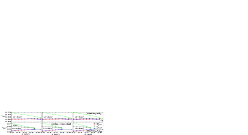
Figure 7: (Color online) Local Fe/Mn 3d rbital occupations for the ddp-model with settings same as Fig. 4.

The general feature of the local d-orbital occupations in the model calculations as shown in Fig. 6 and 7 is consistent with that of the $z^{2}$-factors described above. While the Hubbard U parameter tends to polarize the orbitals, the Hund’s rule coupling J favors the equalization of the local orbital occupations. All local d-orbitals become half occupied as the system approaches the Mott transition for the models of BaMn₂Fe₂ which has 5 electrons in each 5 Mn 3d orbitals. For the BaFe₂As₂ system, there is 6 electrons in each 5 Fe 3d orbitals. Hence we expect an orbital selective Mott transition would occur with large $U$ and $J$Anisimov02 ; Koga04 . We did perform model calculations at even larger $U$ and find an orbitally selective transition where the $z$ factors of all orbitals except the $d_{xy}$-orbital vanish, while $z_{xy}^{2}=1$ as the orbital becomes completely filled. This behavior requires however unphysically large values of $U$. Indeed some signature can be identified as one can see that $n_{x^{2}-y^{2}}^{0}$ becomes closest to 0.5 and $z_{x^{2}-y^{2}}^{2}$ drops most rapidly with increasing $U$ and $J$ for the Fe d-model. When comparing the results of Mn/Fe d-model and the ddp-model, a similar systematic shift of the local orbital occupation curves to the large $J$ side is observed due to the screening and hybridization effect. We conclude that BaMn₂Fe₂ is approaching a Mott insulator with large localized moment. Combining our calculations in the magnetically ordered state and in the paramagnetic state we obtain $J\simeq 0.2-0.3$eV to yields the experimentally observed ordered moment, values that are not yet in the Mott insulating regime, yet they are rather close. In contrast, BaFe₂As₂ is significantly away from Mott localization, yet there are clearly visible polarizations of the orbital populations that demonstrate that the system is in an intermediate regime. To demonstrate that this is indeed the case we determined the quasiparticle weight of a system with the tight binding parameters (ddp-model) of BaFe₂As₂, yet with a total electron count of 11 per Fe atom as appropriate for BaMn₂As₂ (see Fig. 8). Now a Mott transition similar to the actual BaMn₂As${}_{2}\$calculation occurs, albeit at a somewhat larger value of $J$.

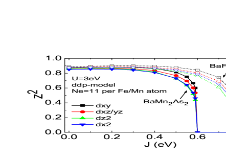
Figure 8: (Color online) The square of the orbital renormalization factor $z_{i\gamma}^{2}$ as a function of Hund’s rule coupling $J$ parameter for the ddp-model of BaMn₂As₂ (solid symbol) and that of BaFe2As2 (open symbol) with total number of electrons fixed to 11 per Fe/Mn atom and U=3eV.

V Effects of charge self-consistency

Figure 9: (Color online) Same as Fig. 4 but based on LDA+G calculations.

Figure 10: (Color online) Local Fe/Mn 3d orbital occupations based on LDA+G calculations with settings same as Fig. 4.

The variation of the $z^{2}$-factors and occupations of the correlated Fe/Mn 3d orbitals with U and J has further been investigated by the LDA+Gutzwiller methodDai08 ; Dai09 , which is built upon the LDA+U approachAnisimov91 ; Anisimov97 . We use the same correlated orbitals obtained via the QUAMBO procedure as in the Fe/Mn d-models for the calculations and achieve the electron density self-consistency. As shown in Fig. 9, the $z^{2}$-curves exhibit a similar trend but vary in a way much slower than that in the Fe/Mn d-models, which can again be attributed to the screening effect of the other electrons in the systems. Our results on the BaFe₂As₂ system are in good agreement with those reported in Ref. Dai10 . Overall, the $z^{2}$-factors for BaMn₂As₂ are systematically smaller than those for BaFe₂As₂. Note that the calculated screened U(J) is 3.6(0.76)eV for Fe and 3.2(0.70)eV for Mn based on the constrained random phase approximation and the maximally localized Wannier functionMiyake08 , it is fairly reasonable to assume that the screened interaction parameters in the models investigated here are also very close. Therefore BaMn₂As₂ is a more correlated material than BaFe₂As₂.

VI Comparative study of the d and ddp model for AFM phase

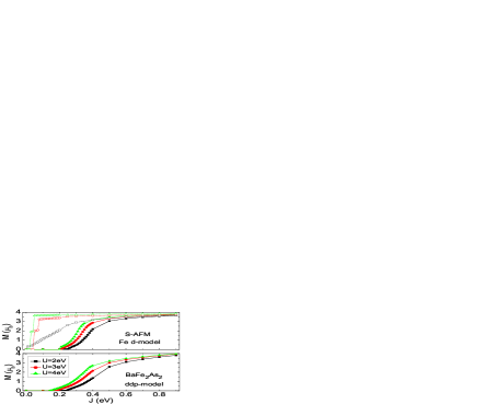
Figure 11: (Color online) Magnetic moment vs J at U=2eV (squares), 3eV (circles) and 4eV (triangles) in the Fe d-model (upper panel) and the ddp-model (lower panel) for BaFe₂As₂. The solid symbols indicate the results using Gutzwiller approximation, and open symbols using Hartree-Fock approximation.

The ground state AFM phase has also been studied for the models of the two systems. Figure 11 shows the behavior of the magnetic moment as a function of J with U fixed at 2eV, 3eV and 4eV in the stripe-type AFM ground state for BaFe₂As₂. In contrast to the Fe d-model including complete local interactions for LaOFeAs in which the system exhibits a sharp transition from PM state to AFM state with large magnetic moment using the Gutzwiller approximationBune11 , the models with only density-density type interactions for BaFe₂As₂ describe the PM-AFM transition fairly well as the magnetic moment increases rapidly yet smoothly when J rises as indicated by the solid symbols in the upper panel. The magnetic moment varies from $0.14\mu_{B}$ to $1.38\mu_{B}$ in the range of $J=0.22-0.32$eV with $U=3$eV. For reference the experimental magnetic moment is $0.87\mu_{B}$ for BaFe₂As₂Huang08 . With the inclusion of the Ba 5d and As 4p orbitals in the ddp-model, the magnetic moment increases slower as seen in the lower panel. The high sensitivity of the magnetic moment to Hund’s rule coupling J is consistent with the DFT+DMFT calculation resultsYin11 . For comparison, Fig. 11 also shows the magnetic moment of the AFM phase in the Fe d-model with Hartree-Fock approximation by the open symbols in the upper panel. Within Hartree-Fock approximation, the PM-AFM transition takes place at much smaller J. The magnetic moment exhibits quite smooth variation with increasing J at U=2eV. However, an abrupt transition from PM to AFM state with large magnetic moment occurs at U=3eV. In comparison, the models of BaMn₂As₂ yield a very sharp transition from PM to the G-type AFM ground state with magnetic moment $M\approx 3\mu_{B}$ as shown in Fig. 12. However, it is still reasonable since the experimental magnetic moment is 3.88$\mu_{B}$Singh091 . The $z^{2}$-factors for the models of BaFe₂As₂ in the AFM ground state are always or order unity ($>0.8$).

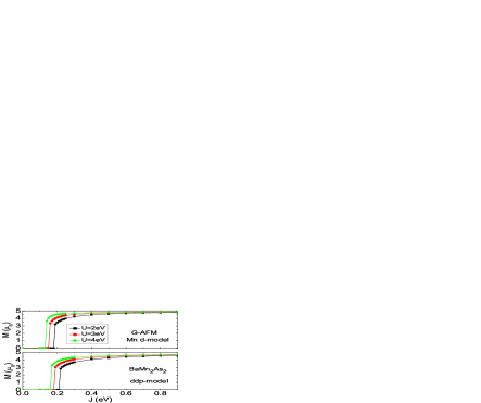
Figure 12: (Color online) Magnetic moment vs J curves for BaMn₂As₂ with setting as as Fig. 11.

VII Conclusion

In summary, we have studied the Fe/Mn d-model and the ddp-model on the electronic and magnetic properties of the BaFe₂As₂ and BaMn₂As₂ systems. The renormalization factors of the correlated Mn 3d orbitals are found to be systematically smaller than those of Fe 3d orbitals, implying that the electron correlation for BaMn₂As₂ are much more efficient to cause Mott localization physics compared to BaFe₂As₂. Ultimately this is due to the fact that Fe, with its close to six electrons, must undergo an orbital selective Mott transition while the odd number of electrons in case of Mn allow for a more ordinary Mott transition. While the strength of the interactions are not sufficient for Mott localization in either system the Mn-based material is significantly closer to localization. The LDA+Gutzwiller results on the paramagnetic phase with electron density self-consistency also confirm the conclusion. The variation of the magnetic moment in the AFM ground state of the two compounds seems in accordance with the experimental results: a smooth increase of the magnetic moment with rising $J$ for the stripe-AFM ground state of BaFe₂As₂ with small experimental magnetic moment and an abrupt jump of the magnetic moment from $0$ to about $3\mu_{B}$ for the G-AFM ground state of BaFe₂As₂ with large experimental magnetic moment.  We also checked that the two different ordered states are indeed energetically lower in the respective systems. The Gutzwiller approximation, however, is not able to provide a quantitatively consistent description of the AFM ground state for the iron pnictide systems with both correct magnetic moment and band renormalization factor for the same parameters. Nevertheless it is a comparatively easy to implement and powerful tool that allows for a first analysis of the role of magnetic correlations, the nature of magnetically ordered states in strongly correlated multi-orbital materials.

- (1) Y. Kamihara, T. Watanabe, M. Hirano, and H. Hosono, Journal of the American Chemical Society 130, 3296-3297 (2008).
- (2) M. Rotter, M. Tegel, and D. Johrendt, Phys. Rev. Lett. 101, 107006 (2008).
- (3) F.-C. Hsu, J.-Y. Luo, K.-W. Yeh, T.-K. Chen, T.-W. Huang, P. M. Wu, Y.-C. Lee, Y.-L. Huang, Y.-Y. Chu, D.-C. Yan, and M.-K. Wu, Proceedings of the National Academy of Sciences 105, 14262-14264 (2008).
- (4) J. H. Tapp, Z. Tang, B. Lv, K. Sasmal, B. Lorenz, P. C. W. Chu, and A. M. Guloy, Phys. Rev. B 78, 060505 (2008).
- (5) M. S. Torikachvili, S. L. Bud’ko, N. Ni, and P. C. Canfield, Phys. Rev. Lett. 101, 057006 (2008).
- (6) X. H. Chen, T. Wu, G. Wu, R. H. Liu, H. Chen, and D. F. Fang, Nature 453, 761-762 (2008).
- (7) Z. Ren, W. Lu, J. Yang, W. Yi, X. Shen, Z. Li, G. Che, X. Dong, L. Sun, F. Zhou, and Z. Zhao, Chinese Physics Letters 25, 2215-2216 (2008).
- (8) Y. Singh, A. Ellern, and D. C. Johnston, Phys. Rev. B 79, 094519 (2009).
- (9) Y. Singh, M. A. Green, Q. Huang, A. Kreyssig, R. J. McQueeney, D. C. Johnston, and A. I. Goldman, Phys. Rev. B 80, 100403 (2009).
- (10) J. An, A. S. Sefat, D. J. Singh, and M.-H. Du, Phys. Rev. B 79, 075120 (2009).
- (11) D. Johnston, Adv. in Phys. 59, 803-1061 (2010).
- (12) I. Mazin, M. D. Johannes, L. Boeri, K. Koepernik, and D. J. Singh, Phys. Rev. B 78, 085104 (2008).
- (13) K. Haule and G. Kotliar, New Journal of Physics 11, 025021 (2009).
- (14) K. Kuroki, S. Onari, R. Arita, H. Usui, Y. Tanaka, H. Kontani, and H. Aoki, Phys. Rev. Lett. 101, 087004 (2008).
- (15) S. Raghu, X.-L. Qi, C.-X. Liu, D. J. Scalapino, and S.-C. Zhang, Phys. Rev. B 77, 220503(R) (2008).
- (16) A. V. Chubukov, D. V. Efremov, and I. Eremin, Phys. Rev. B 78, 134512 (2008).
- (17) V. Cvetkovic and Z. Tesanovic, Europhys. Lett. 85, 37002 (2009).
- (18) H. Zhai, F. Wang, and D.-H. Lee, Phys. Rev. B 80, 064517 (2009).
- (19) R. Sknepnek, G. Samolyuk, Y.-b. Lee, and J. Schmalian, Phys. Rev. B 79, 054511 (2009).
- (20) Z. P. Yin, K. Haule, and G. Kotliar, Nat Phys 7, 294-297 (2011).
- (21) Z. P. Yin, K. Haule, and G. Kotliar, to appear in Nature Materials (2011).
- (22) G. Wang, Y. Qian, G. Xu, X. Dai, and Z. Fang, Phys. Rev. Lett. 104, 047002 (2010).
- (23) S. Zhou and Z. Wang, Phys. Rev. Lett. 105, 096401 (2010).
- (24) T. Schickling, F. Gebhard, and J. Bünemann, Phys. Rev. Lett. 106, 146402 (2011).
- (25) T. Schickling, F. Gebhard, J. Bünemann, L. Boeri, O. K. Andersen, W. Weber, arXiv:1109.0929
- (26) M. C. Gutzwiller, Phys. Rev. Lett. 10, 159 (1963).
- (27) M. C. Gutzwiller, Phys. Rev. 137, A1726 (1965).
- (28) J. Bünemann and F. Gebhard, Phys. Rev. B 76, 193104-4 (2007).
- (29) G. Kotliar and A. E. Ruckenstein, Phys. Rev. Lett. 57, 1362 (1986).
- (30) X. Y. Deng, X. Dai, and Z. Fang, EPL (Europhysics Letters) 83, 37008 (2008).
- (31) X. Y. Deng, L. Wang, X. Dai, and Z. Fang, Phys. Rev. B 79, 075114-20 (2009).
- (32) V. I. Anisimov, I. V. Solovyev, M. A. Korotin, M. T. Czyzdotyk, and G. A. Sawatzky, Phys. Rev. B 48, 16929 (1993).
- (33) M. T. Czyżyk and G. A. Sawatzky, Phys. Rev. B 49, 14211 (1994).
- (34) G. Kotliar, S. Y. Savrasov, K. Haule, V. S. Oudovenko, O. Parcollet, and C. A. Marianetti, Rev. Mod. Phys. 78, 865 (2006).
- (35) Y. X. Yao, C. Z. Wang, and K. M. Ho, Phys. Rev. B 83, 245139 (2011).
- (36) K. M. Ho, J. Schmalian, and C. Z. Wang, Phys. Rev. B 77, 073101 (2008).
- (37) J. Bünemann, F. Gebhard, and R. Thul, Phys. Rev. B 67, 075103 (2003).
- (38) M. Rotter, M. Tegel, D. Johrendt, I. Schellenberg, W. Hermes, and R. Pöttgen, Phys. Rev. B 78, 020503 (2008).
- (39) W. C. Lu, C. Z. Wang, T. L. Chan, K. Ruedenberg, and K. M. Ho, Phys. Rev. B 70, 041101 (2004).
- (40) T. L. Chan, Y. X. Yao, C. Z. Wang, W. C. Lu, J. Li, X. F. Qian, S. Yip, and K. M. Ho, Phys.Rev.B 76, 205119 (2007).
- (41) X. F. Qian, J. Li, L. Qi, C. Z. Wang, T. L. Chan, Y. X. Yao, K. M. Ho, and S. Yip, Phys.Rev.B 78, 245112 (2008).
- (42) Y. X. Yao, C. Z. Wang, G. P. Zhang, M. Ji, and K. M. Ho, Journal of Physics-Condensed Matter 21, 235501 (2009).
- (43) E. Aktürk and S. Ciraci, Phys. Rev. B 79, 184523 (2009).
- (44) N. Marzari, and D. Vanderbilt, Phys.Rev.B 56, 12847 (1997).
- (45) I. Souza, N. Marzari, and D. Vanderbilt, Phys.Rev.B 65, 035109 (2001).
- (46) S. Graser, A. F. Kemper, T. A. Maier, H.-P. Cheng, P. J. Hirschfeld, and D. J. Scalapino, Phys. Rev. B 81, 214503 (2010).
- (47) V. I. Anisimov, I. A. Nekrasov, D. E. Kondakov, T. M. Rice, and M. Sigrist, The European Physical Journal B - Condensed Matter and Complex Systems 25, 191-201 (2002).
- (48) A. Koga, N. Kawakami, T. M. Rice, and M. Sigrist, Phys. Rev. Lett. 92, 216402 (2004).
- (49) V. I. Anisimov, J. Zaanen, and O. K. Andersen, Phys. Rev. B 44, 943 (1991).
- (50) V. I. Anisimov, F. Aryasetiawan, and A. Lichtenstein, Journal of Physics-condensed Matter 9, 767-808 (1997).
- (51) T. Miyake and F. Aryasetiawan, Phys. Rev. B 77, 085122-9 (2008).
- (52) Q. Huang, Y. Qiu, W. Bao, M. A. Green, J. W. Lynn, Y. C. Gasparovic, T. Wu, G. Wu, and X. H. Chen, Phys. Rev. Lett. 101, 257003 (2008).
- (53) P. Richard, K. Nakayama, T. Sato, M. Neupane, Y.-M. Xu, J. H. Bowen, G. F. Chen, J. L. Luo, N. L. Wang, X. Dai, Z. Fang, H. Ding, and T. Takahashi, Phys. Rev. Lett. 104, 137001 (2010).