Comprehensive abundance analysis of red giants in the open clusters NGC 752, NGC 1817, NGC 2360 and NGC 2506^⋆

Abstract

We have analyzed high-dispersion echelle spectra ($R\ga 50,000$) of red giant members for four open clusters to derive abundances for many elements. The spread in temperatures and gravities being very small among the red giants nearly the same stellar lines were employed thereby reducing the random errors. The errors of average abundance for the cluster were generally in 0.02 to 0.07 dex range. Our present sample covers galactocentric distances of 8.3 to 10.5 kpc. The [Fe/H] values are $-$0.02$\pm$0.05 for NGC 752, $-$0.07$\pm$0.06 for NGC 2360, $-$0.11$\pm$0.05 for NGC 1817 and $-$0.19$\pm$0.06 for NGC 2506. Abundances relative to Fe for elements from Na to Eu are equal within measurement uncertainties to published abundances for thin disk giants in the field. This supports the view that field stars come from disrupted open clusters.

1 Introduction

Open clusters (OCs) are believed to be coeval groups of stars born from the same proto-cluster cloud which may have been part of a larger star-forming region in the Milky Way. Ages of clusters range from very young where stars are still forming to nearly 10 Gyr (Dias et al. 2002). Since all stars in most OCs are at the same distance and have the same chemical composition, basic stellar parameters like age, distance, and metallicity can be determined more accurately than for field stars. Thus, OCs provide an excellent opportunity to map the structure, kinematics, and chemistry of the Galactic disk with respect to Galactic coordinates and time.

The presence of chemical homogeneity among cluster members has been shown by the study of OCs, see, for example, spectroscopic analyses of the Hyades (Paulson et al. 2003; De Silva et al. 2006) and Collinder 261 (Carretta et al. 2005; De Silva et al. 2007). This observed homogeneity signifies that the proto-cloud is well mixed, and hence, the abundance pattern of a cluster bears the signature of chemical evolution of the natal cloud. Chemical evolution of the Milky Way has, of course, been well studied using field stars. A large fraction of field stars are from disrupted OCs (Lada & Lada 2003). The youngest OCs may be intact. The oldest OCs may be totally disrupted. Thus, the field stars do not fully sample the age distribution of OCs and, in particular, the youngest stellar generations are under-represented by field stars.

In this paper, we report abundance analyses from high-resolution spectra of red giants in four OCs: NGC 752, NGC 1817, NGC 2360, and NGC 2506. These analyses are the first for these OCs to report elemental abundances for elements from Na to Eu.

The structure of the paper is as follows: In Section 2 we describe the data selection, observations and data reduction and Section 3 is devoted to the abundance analysis. In Section 4 we present our results and compare them with the abundances derived from samples of field thin and thick disk stars (i.e. dwarfs and giants). Finally, in Section 5 we give the conclusions.

Table 1: Target clusters and their properties from the literature.

Cluster	l	b	Age	[Fe/H]phot.	Rgc	(m-M)v	E(B-V)	[Fe/H]ref
	(deg.)	(deg.)	(Gyr)	(dex.)	(kpc)	(mag.)	(mag.)
NGC 752	137.12	$-$23.25	1.12	$-$0.12	8.3	8.18	0.03	Bartašiūtė et al. (2007)
NGC 1817	186.16	$-$13.09	0.41	$-$0.33	9.9	11.79	0.25	Parisi et al. (2005)
NGC 2360	229.81	$-$01.43	0.56	$-$0.12	9.3	11.72	0.11	Claria et al. (2008)
NGC 2506	230.56	$+$09.93	1.11	$-$0.32	10.5	12.95	0.08	Henderson et al. (2007)

Table 2: The observed stars.

Cluster	Star ID	$\alpha(2000.0)$	$\delta(2000.0)$	V	B-V	$RV_{helio}$	S/N
		(hh mm s)	($\degr$ $\arcsec$ $\arcmin$)	(mag.)	(mag.)	(km s-1)	at 6000 Å
NGC 752	77	01 56 21.60	37 36 08.00	9.35	$+$1.02	+6.3$\pm$0.2	100
	137	01 57 03.10	38 08 02.00	8.89	$+$1.02	+5.9$\pm$0.2	100
	295	01 58 29.80	37 51 37.00	9.29	$+$0.96	+6.3$\pm$0.2	120
	311	01 58 52.90	37 48 57.00	9.04	$+$1.03	+6.7$\pm$0.2	120
NGC 1817	1027	05 12 19.38	16 40 48.64	12.13	$+$1.03	+66.1$\pm$0.2	110
	2038	05 12 06.27	16 38 15.34	12.17	$+$1.12	+66.6$\pm$0.2	90
	2059	05 12 24.65	16 35 48.84	12.04	$+$1.08	+66.5$\pm$0.2	90
NGC 2360	5	07 18 14.13	$-$15 37 30.49	10.74	$+$1.04	+30.4$\pm$1.1	77
	6	07 18 19.08	$-$15 37 32.62	11.03	$+$1.04	+29.1$\pm$0.1	95
	8	07 18 10.84	$-$15 34 13.30	11.09	$+$1.01	+29.2$\pm$0.2	80
	12	07 18 09.58	$-$15 31 39.80	10.34	$+$1.16	+29.5$\pm$0.4	75
NGC 2506	2212	08 00 08.68	$-$10 46 37.50	11.95	$+$1.07	+84.1$\pm$0.2	50
	3231	07 59 55.77	$-$10 48 22.73	13.12	$+$0.98	+84.9$\pm$0.4	45
	4138	08 00 01.49	$-$10 45 38.50	13.30	$+$0.91	+84.9$\pm$0.3	60

2 Observations and data reduction

Clusters were selected from the New catalogue of optically visible open clusters and candidates (Dias et al. 2002). Emphasis was placed on OCs not yet subjected to high resolution spectroscopy. Since the main sequence stars in the chosen OCs were faint, we elected to observe the red giant members. For each of the target clusters, red giants were selected using the WEBDA database. Target clusters and their properties are shown in the Table 1: column 1 represents the cluster name, columns 2 & 3 the Galactic longitude and latitude in degrees, column 4 the age, column 5 the photometric estimate of the iron abundance, column 6 the Galactocentric distance, column 7 the distance modulus, column 8 the reddening, column 9 the reference to [Fe/H]. All quantities are from the database entry except for the [Fe/H] abundance and the Galactocentric distance, Rgc, which we calculate assuming a distance of the Sun from the Galactic centre of 8.0$\pm$0.6 kpc (Ghez et al. 2008) .

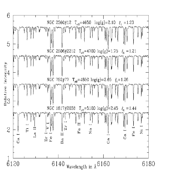
Figure 1: Representative spectra for the four clusters.

Observations were conducted during February 6-10, 1999 with Tull echelle coudé spectrograph (Tull et al. 1995) on the 2.7-m Harlan J. Smith telescope at the McDonald observatory. Spectra are at a resolving power of $\ga$50,000 as measured by the FWHM of Th I lines in comparison spectra. The spectral coverage was complete from 4000 Å  to 5600 Å  and substantial but incomplete from 5600 Å  to about 9800 Å. A series of bias and flat frames were obtained at several exposure levels chosen to match those of the program stars, and comparison Th-Ar spectra were taken to establish the wavelength scale. We obtained on each night the spectrum of a rapidly-rotating B star to monitor the presence of telluric lines.

Spectroscopic reductions were done with the ${\bf IRAF}$ software of $NOAO$ within the imred and echelle packages, involving bias subtraction, scattered light correction, flat-fielding, wavelength calibration and continuum fitting. We measured the radial velocity (RV) of each star on each spectrum. The continuum-fitted spectrum was corrected for the Doppler shift using the routine dopcor available in IRAF task splot. Our radial velocity measurements are in fair agreement with the previous radial velocity measurements for the red giants in OCs (Mermilliod et al. 2008).

The identification and basic observational data for the stars observed in each of the clusters are given in Table 2, along with the computed radial velocity and S/N of each of the spectra extracted at 6000 Å for each of the stars. Spectra of a representative region are shown in Figure 1 for one star from each of the four clusters.

3 Abundance analysis

3.1 Line selection

Selection of stellar lines which are free from blends is crucial for deriving accurate elemental abundances. We used Rowland’s preliminary table of solar spectrum wavelengths (Moore et al. 1966) and the the Arcturus spectrum (Hinkle et al. 2000) to identify unblended spectral lines. We employed strict criteria in the selection of suitable lines. First, in order to avoid the difficulty in defining the continuum due to heavy line crowding in the blue part of the spectrum, we selected lines only within the 4300 to 7850 Å wavelength range. Second, regions containing telluric absorption lines were generally avoided. Third, lines which appear asymmetric were assumed to be blended with unidentified lines and discarded. Fourth, lines with equivalent widths (EWs) below 10 mÅ were rejected because they are too sensitive to noise and the normalization of the continuum, and lines with equivalent widths greater than 230 mÅ were discarded because they are too saturated.

Application of our criteria resulted in a list of 55 Fe I lines with lower excitation potentials (LEP) ranging from 0.9 to 5.0 eV and EWs of up to 180 mÅand 10 Fe II lines with excitation potentials of 2.8 to 3.9 eV and EWs up to 120 mÅ.

A portion of final linelist with solar EWs is given in Table 3 with details about the lines including the $\log$ gf’s (see below). For each line in the constructed linelist, we provide a gf-value from the literature. In most cases, we located recent experimental determinations or chose values from critical reviews. References to the adopted sources are given in Table 3. EWs were measured manually using the task ’splot’ contained in IRAF by fitting a Gaussian profile to the observed line.

For several absorption features, multiple components of a given atomic transition contribute to the feature. In such cases, we computed a synthetic spectrum including all components and occasionally other lines too and matched the synthetic spectrum to the observed spectrum by varying the abundance of the element in question.

As a check on the chosen gf-values, we derived solar abundances using the ATLAS9 model for $T_{eff}$ = 5777 K, log $g$=4.44 cgs. A microturbulence of $\xi_{t}$ = 0.95 km s^-1 was found from iron lines. Solar equivalent widths were measured off the solar integrated disk spectrum (Kurucz et al. 1984). Abundances are given in Table 4 along with those from the recent review by Asplund et al. (2009). Our abundances for the majority of elements are in good agreement with Asplund et al.’s. Small differences in abundances are inevitable, for example, the line lists are not necessarily identical as to selected lines and/or gf-values and the adopted solar models are different; ours is a classical model but Asplund et al. for many elements use a model representing the solar granulation. For the purposes of determining the stellar abundances, we adopt our solar abundances when computing [X/H] and [X/Fe], i.e., our analysis is essentially a differential one relative to the Sun.

Table 3: Adopted linelist. All the columns are self-explanatory.

Atom	Wavelength	LEP1	$\log~{}{gf}$	$W_{\lambda,\odot}$	$Ref^{a}$.
	( Å)	(eV)		(mÅ)
Na I	4668.567	2.100	-1.31	53.4	NIST
	4982.821	2.100	-0.96	79.0	NIST
	5688.210	2.100	-0.45	115.4	NIST
	6154.224	2.100	-1.55	36.3	NIST
	6160.746	2.100	-1.25	55.9	NIST
Mg I	5711.090	4.340	-1.72	104.5	NIST
	6318.708	5.108	-1.90	42.9	NIST
Al I	7084.564	4.020	-0.93	21.4	KUR
	7835.296	4.020	-0.65	41.2	KUR
	7836.119	4.020	-0.47	55.4	KUR
Si I	5665.551	4.920	-2.04	39.4	NIST
	5645.606	4.930	-2.14	34.9	LUCK
	5701.100	4.930	-2.05	37.7	NIST
	5753.632	5.610	-1.30	42.5	LUCK
	6131.570	5.610	-1.70	22.3	LUCK
	6131.851	5.610	-1.62	23.3	LUCK
	6145.013	5.610	-1.48	36.5	LUCK
	6237.319	5.610	-1.14	56.7	LUCK
	6244.470	5.610	-1.36	45.1	LUCK
	6243.812	5.613	-1.26	46.5	KUR
	6142.486	5.620	-1.54	33.0	LUCK
	6721.840	5.862	-1.06	42.8	LUCK
	6195.445	5.873	-1.80	14.9	LUCK
Ca I	6122.221	1.890	-0.32	161.9	LUCK
	5581.971	2.520	-0.55	93.7	LUCK
	5590.117	2.520	-0.57	91.7	LUCK
	6166.434	2.520	-1.14	69.2	LUCK
	6169.560	2.520	-0.48	108.5	LUCK
	6455.599	2.520	-1.29	56.2	LUCK
	6499.649	2.520	-0.82	85.0	LUCK
	6471.662	2.526	-0.68	90.7	LUCK
Sc I	5686.832	1.440	0.38	8.3	LUCK
	5356.090	1.860	0.17	2.3	LUCK
Sc II	6604.587	1.357	-1.31	35.1	NIST
	5667.141	1.500	-1.20	30.0	KUR
	6245.615	1.507	-1.03	35.4	KUR
	6300.681	1.507	-1.89	8.1	KUR
	5526.813	1.768	0.06	75.6	KUR
Ti I	5039.960	0.021	-1.13	75.7	NIST
	5460.497	0.048	-2.75	9.6	LUCK
	4999.510	0.826	0.31	103.6	LUCK
	5020.026	0.836	-0.35	72.6	KUR
	5295.776	1.067	-1.63	13.1	NIST
	5474.223	1.460	-1.23	10.8	NIST
	5490.148	1.460	-0.93	21.6	NIST
	4617.274	1.749	0.39	61.2	NIST
	5739.980	2.236	-0.60	7.3	NIST
	5702.656	2.292	-0.57	8.1	NIST
Ti II	4764.528	1.237	-2.77	37.2	LUCK
	4708.665	1.240	-2.21	52.9	NIST
	5005.168	1.566	-2.54	25.5	NIST
	5381.022	1.566	-1.85	57.3	LUCK
	5396.244	1.580	-2.92	12.1	LUCK
	5336.788	1.582	-1.70	69.2	NIST
	5418.767	1.582	-1.99	48.1	KUR
V I	6251.823	0.286	-1.34	15.8	NIST
	6111.647	1.043	-0.71	10.7	NIST
	5727.653	1.051	-0.87	8.9	NIST
	6135.366	1.051	-0.75	10.4	NIST
	5737.062	1.064	-0.74	10.8	NIST
	5668.365	1.081	-1.03	5.6	NIST
	5670.848	1.081	-0.42	19.0	NIST
	5727.044	1.081	-0.01	39.9	NIST

Table 4: Solar abundances derived by employing the solar model atmosphere from Castelli & Kurucz (2003) compared with the photospheric abundances from Asplund et al. (2009).

Species	$\log~{}\epsilon_{\odot}$	$\log~{}\epsilon_{\odot}$
	(our study)	(Asplund)
Na I	6.29$\pm$0.03(5)	6.24$\pm$0.04
Mg I	7.55$\pm$0.06(2)	7.60$\pm$0.04
Al I	6.35$\pm$0.06(3)	6.45$\pm$0.03
Si I	7.55$\pm$0.05(2)	7.51$\pm$0.03
Ca I	6.28$\pm$0.05(8)	6.34$\pm$0.04
Sc I	2.98$\pm$0.03(2)	3.15$\pm$0.04
Sc II	3.17$\pm$0.05(5)
Ti I	4.88$\pm$0.06(10)	4.95$\pm$0.05
Ti II	4.92$\pm$0.09(7)
V I	3.94$\pm$0.05(8)	3.93$\pm$0.08
Cr I	5.59$\pm$0.04(12)	5.64$\pm$0.04
Cr II	5.67$\pm$0.05(6)
Mn I	5.39	5.43$\pm$0.04
Fe I	7.54$\pm$0.05(36)	7.50$\pm$0.04
Fe II	7.52$\pm$0.05(13)
Co I	4.86$\pm$0.03(5)	4.99$\pm$0.07
Ni I	6.24$\pm$0.02(14)	6.22$\pm$0.04
Cu I	4.18	4.19$\pm$0.04
Zn I	4.59$\pm$0.00(2)	4.56$\pm$0.05
Y II	2.19$\pm$0.07(5)	2.21$\pm$0.05
Zr I	2.59$\pm$0.11(2)	2.58$\pm$0.04
Ba II	2.13	2.18$\pm$0.09
La II	1.24$\pm$0.13(2)	1.10$\pm$0.04
Ce II	1.56	1.58$\pm$0.04
Nd II	1.50$\pm$0.09(3)	1.42$\pm$0.04
Sm II	1.00	0.96$\pm$0.04
Eu II	0.51	0.52$\pm$0.04

3.2 Determination of atmospheric parameters

3.2.1 Photometry

Initial estimates of the effective temperature of a red giant were derived from dereddened B and V photometry using the empirically-calibrated colour-temperature relation by Alonso et al. (1999) based on a large sample of field and globular cluster giants of spectral types from F0 to K5. An error of 3% is expected in the derived temperatures.

Gravities were computed using the known distance to the OCs, temperature and bolometric corrections, and the cluster turn-off mass. We have adopted a turn-off mass of 1.5M_⊙ for NGC 752 (Bartasiute et al. 2007), 2M_⊙ for NGC 1817 (Jacobson et al. 2009), 1.98M_⊙ for NGC 2360 (Hamdani et al. 2000), and 1.69M_⊙ for NGC 2506 (Carretta et al. 2004). The relation between log $g$ and T_eff is given by (Allende Prieto et al. 1999)

$\log{g_{\star}}$= $\log{g}_{\odot}$+$\log(M_{\star}/M_{\odot})$+4 $\log(T_{eff}/T_{eff}{\odot})$

$$+0.4(V_{0}+BC_{V})+2log{\pi}+0.12$$ (1)

with the corresponding luminosity given by

$$log(L_{*}/L_{\odot})=-[0.4(V_{0}+BC_{V})+2log~{}{\pi}+0.12]$$ (2)

where $\pi$ is the parallax, V₀ is the apparent Johnson V magnitude corrected for reddening, and BC_V is the bolometric correction. We adopt log g_⊙= 4.44, T${}_{eff},_{\odot}$= 5777 K. Bolometric corrections were taken from the calibration by Alonso et al. (1999).

We suppose that the errors in different quantities involved in equation (1) are independent of each other. Then, by assuming an error of 10% in the stellar mass, an uncertainty of 3% in T_eff, an uncertainty of 5% in photometric V magnitude and the bolometric corrections, and an error of 10% in parallax, we get an error of $\simeq$ 0.11 dex in $\log~{}g$ and the corresponding uncertainty in $\log~{}L_{*}$ amounts to 0.08.

3.2.2 Spectroscopy

The spectroscopic abundance analysis was performed with the 2010 version of the local thermodynamical equilibrium (LTE) line synthesis program MOOG (Sneden 1973). Model atmospheres were generated by linear interpolation from the ATLAS9 model atmosphere grid (Castelli & Kurucz 2003). A model atmosphere is characterized by the effective temperature T_eff, the surface gravity $\log~{}{g}$, microturbulence velocity $\xi_{t}$, and composition. These models use the classical assumptions of line-blanketed plane-parallel uniform atmospheres in LTE and hydrostatic equilibrium with flux conservation.

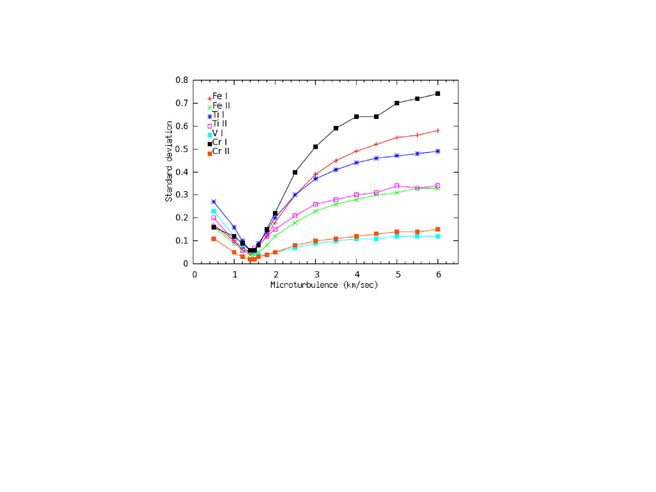
Figure 2: The standard deviation for various species about the mean abundances as a function of microturbulence for the star NGC 752 #311.

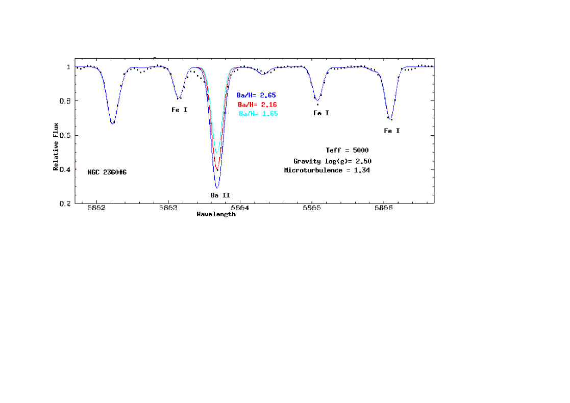
Figure 3: Synthetic spectra and the observed spectrum of NGC 2360 #6 around the Ba II line at 5853 Å. The indicated abundances in the figure are on a logarithmic scale.

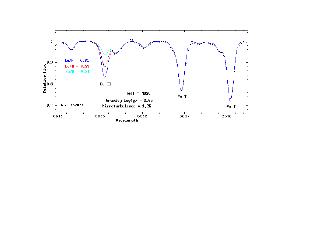
Figure 4: Synthetic spectra and the observed spectrum of NGC 752 #77 around the Eu II line at 6645 Å. The indicated abundances in the figure are on a logarithmic scale.

Spectroscopically, we determine the stellar parameters in the conventional way when LTE is the paramount assumption. The key lines are those of Fe I and Fe II for which we take gf-values from Fuhr & Wiese (2006) and Meléndez & Barbuy (2009). The microturbulence assumed to be isotropic and depth independent is determined from Fe II lines by the requirement that the abundance be independent of a line’s EW. A model atmosphere with the photometrically determined parameters was used initially for this determination. The effective temperature is found by imposing the requirement that the Fe abundance from Fe I lines be independent of a line’s lower excitation potential. Finally, the surface gravity is found by requiring that Fe I and Fe II lines give the same Fe abundance for the derived effective temperature and microturbulence.

A check on the microturbulence is provided by lines of species other than Fe I. For example, for the star NGC 752 #311 we show in Figure 2 the dispersion of the abundance computed from the Fe I, Fe II, Ti I, Ti II, V I, Cr I and Cr II lines as the micorturbulence is varied over the range in the microturbulence, $\xi_{t}$, from 0 to 6 km s^-1. It is clear that the minimum value of dispersion for all species is in the range 1.2-1.6 km s^-1. Thus, we adopt a microturbulence of 1.45 km s^-1 with an uncertainty of 0.20 km s^-1.

Several elements other than Fe provide both neutral and ionized lines and so offer a check on the condition of ionization equilibrium of Fe. Consider for example the four giants from NGC 752: the abundance differences [X/H] between neutral and ionized lines of Sc, Ti, V and Cr are on average 0.03, -0.03, -0.01, and -0.05 dex, respectively where $\pm$0.05 dex corresponds to a change of $logg$ by $\mp$ of 0.15.

The uncertainties in the derived surface temperatures from spectroscopy are provided by the errors in the slope of the relation between the Fe I abundance and LEP of the lines. A perceptible change of slope occures for variations of the temperature from 50$-$100 K about the adopted model.

Therefore, the typical errors considered in this analysis are 100 K in $T_{eff}$, 0.25 cm s^-2 in log $g$ and 0.20 km s^-1 in $\xi_{t}$.

The derived stellar parameters for program stars in each of the cluster are given in Table 5: column 1 represents the cluster name, column 2 the star ID, columns 3 & 4 the photometric T_eff and log $g$ values, columns 5-7 the spectroscopic T_eff, log $g$ and $\xi_{t}$ estimates. Finally, the spectroscopic and photometric luminosities ( log(L/L${}_{\odot})$) are presented in columns 8 & 9. Photometric and spectroscopic estimates are in excellent agreement. Mean differences in T_eff, log $g$ and logL/L_⊙ across the 14 stars are $-28\pm 105$ K, $0.06\pm 0.10$ cgs, and $-0.08\pm 0.10$, respectively. The corresponding comparison of the spectroscopic with the photometric [Fe/H] in Table 1 also illustrates fair agreement: $\Delta$[Fe/H] = 0.09 (NGC 752), 0.21 (NGC 1817), 0.05 (NGC 2360), and 0.12 (NGC 2506).

Table 5: Basic photometric and spectroscopic atmospheric parameters for the stars in each cluster.

Cluster	Star ID	$T_{eff,phot}$	$\log g_{phot}$	$T_{eff,spec}$	$\log g_{spec}$	$\xi_{spec}$	$\log(L/L_{\odot})$	$\log(L/L_{\odot})$
		(K)	(cm s-2)	(K)	(cm s-2)	(km sec-1)	spectroscopy	photometry
NGC 752	77	4780	2.75	4850	2.65	1.26	1.71	1.54
	137	4780	2.57	4850	2.50	1.36	1.81	1.72
	295	4899	2.80	5050	2.85	1.47	1.53	1.53
	311	4761	2.62	4850	2.60	1.45	1.71	1.66
NGC 1817	1027	5177	2.66	5100	2.60	1.39	1.92	1.89
	2038	4968	2.57	5100	2.45	1.44	2.07	1.90
	2059	5059	2.57	4800	2.40	1.38	2.01	1.94
NGC 2360	5	4899	2.56	4900	2.70	1.29	1.75	1.89
	6	4899	2.68	5000	2.50	1.34	1.98	1.77
	8	4962	2.74	5050	2.60	1.37	1.90	1.74
	12	4668	2.27	4650	2.10	1.23	2.26	2.10
NGC 2506	2212	4710	1.86	4700	1.75	1.21	2.56	2.45
	3231	4893	2.44	5000	2.50	1.42	1.92	1.94
	4138	5048	2.60	5100	2.60	1.47	1.85	1.84

3.3 Synthetic spectra

We compared the stellar spectra to the synthetic spectra to derive abundances for the lines having intrinsic multiple components and lines affected by blends. Figures 3 and 4 show synthetic spectra fit to the observed one using three different abundances. The dotted line is the stellar spectrum. The red line is the best fit to the stellar spectrum, with the other lines representing different values for [Ba/H] and [Eu/H] abundances, based on $\chi^{2}$ goodness of fit provided by MOOG.

In this analysis, we have adopted the hfs data of Prochaska & McWilliam (2000) for the synthesis of Mn I line at 6013 Å, Allen et al. (2011) for Cu I line at 5218 Å, McWilliam (1998) for Ba II line at 5853 Å and Mucciarelli et al. (2008) for Eu II line 6645 Å. Isotopic ratios for Cu I, Ba II and Eu II were taken from Lodders (2003). Further, we have synthesized the lines Ce II line at 5472 Å and Sm II line at 4577 Å since the blends make it impossible to measure their EWs. The spectrum synthesis was carried out by running the MOOG in ’synth’ mode.

Since all odd species exhibit hfs effects of relatively varying strengths, we have performed spectrum synthesis over Sc II line at 6245 Å  V I line at 5727 Å and Co I line at 5647 Å . Here, we have adopted the hfs data of Prochaska & McWilliam (2000) for Sc II and for V I and Co I hfs components were taken from Kurucz linelists. We noticed that the these lines are not severely effected by hfs effects, causing an abundance difference of 0.0$-$0.10 dex with and without the inclusion of hfs components, and negligible while considering the standard deviation around mean what we obtain in the fine analysis using the routine ’abfind’ in MOOG.

3.4 Abundances

The abundance analysis was conducted with the model atmospheres having the stellar parameters determined from the spectra (Table 2), the line list (Table 12) and the program MOOG. Abundances [X/H] are expressed relative to the solar abundances derived from the adopted gf-values. Results for the individual stars in each of the OCs are given in Tables 8, 9, 10, and 11.

For each abundance based on analysis of EWs, the abundance and the standard deviation were calculated from all lines of a given species. The tables give the abundances of [Fe/H] and [X/Fe] for all elements. The quantity [X/Fe] minimizes the sensitivity to errors in the model atmosphere arising from uncertainties affecting the stellar parameters. Inspection of the Tables 8-11 shows that, in general, the compositions [X/Fe] of stars in a given cluster are generally identical to within the (similar) standard deviations computed for an individual star. Exceptions tend to occur for species represented by few lines, as expected when the uncertainty in measuring equivalent widths is a contributor to the total uncertainty. From the spread in the abundances for the stars of a given cluster we obtain the standard deviation $\sigma_{1}$ in the Tables 8-11 in the column headed ‘average’. Errors in the adopted gf values are unimportant when providing differential abundances ([X/H] or [X/Fe]) provided that the solar and stellar abundances depend on the same set of lines.

Table 6: Sensitivity of abundances to the uncertainties in the model parameters for the star 5 in NGC 2360 with $T_{eff}$= 4900 K, $\log{g}$= 2.70 cm s^-2,and $\xi_{t}$= 1.29 km s^-1.

	$T_{eff}\pm$100 K	$\log~{}{g}\pm$ 0.25	$\xi_{t}\pm$ 0.20
Species	$\sigma_{T_{eff}}$	$\sigma_{log{g}}$	$\sigma_{\xi_{t}}$	$\sigma_{2}$
Na I	$+0.06/-0.07$	$-0.01/+0.01$	$-0.06/+0.06$	0.05
Mg I	$+0.05/-0.05$	$-0.05/+0.05$	$-0.06/+0.05$	0.05
Al I	$+0.03/-0.04$	$-0.02/0.00$	$-0.03/+0.03$	0.03
Si I	$-0.03/+0.04$	$+0.04/-0.06$	$-0.02/+0.03$	0.04
Ca I	$+0.08/-0.08$	$-0.01/0.00$	$-0.11/+0.11$	0.08
Sc I	$+0.14/-0.15$	$+0.01/-0.01$	$-0.02/+0.03$	0.08
Sc II	$-0.03/+0.04$	$+0.11/-0.13$	$-0.06/+0.07$	0.08
Ti I	$+0.12/-0.12$	$+0.01/+0.01$	$-0.06/+0.07$	0.08
Ti II	$-0.04/+0.05$	$+0.11/-0.14$	$-0.14/+0.15$	0.11
V I	$+0.14/-0.14$	$+0.02/0.00$	$-0.05/+0.07$	0.08
Cr I	$+0.08/-0.09$	$0.00/0.00$	$-0.09/+0.08$	0.07
Cr II	$-0.09/+0.09$	$+0.10/-0.14$	$-0.06/+0.06$	0.09
Mn I	$-0.09/+0.09$	$+0.01/-0.02$	$-0.13/+0.13$	0.09
Fe I	$+0.04/-0.04$	$+0.02/-0.03$	$-0.10/+0.10$	0.06
Fe II	$-0.11/+0.12$	$+0.13/-0.16$	$-0.08/+0.10$	0.12
Co I	$+0.05/-0.03$	$+0.05/-0.04$	$-0.05/+0.06$	0.05
Ni I	$+0.02/-0.01$	$+0.05/-0.06$	$-0.08/+0.09$	0.06
Cu I	$+0.01/-0.01$	$+0.04/-0.05$	$-0.06/+0.06$	0.04
Zn I	$-0.07/+0.07$	$+0.07/-0.10$	$-0.15/+0.15$	0.11
Y II	$-0.02/+0.01$	$+0.11/-0.13$	$-0.07/+0.08$	0.08
Zr I	$+0.17/-0.19$	$0.00/+0.01$	$-0.02/+0.01$	0.10
Ba II	$-0.01/+0.03$	$+0.12/-0.14$	$-0.21/+0.23$	0.15
La II	$+0.01/0.00$	$+0.11/-0.12$	$-0.03/+0.05$	0.07
Ce II	$+0.01/0.00$	$+0.11/-0.12$	$-0.02/+0.02$	0.07
Nd II	$0.00/0.00$	$+0.11/-0.12$	$-0.03/+0.04$	0.07
Sm II	$+0.01/0.00$	$+0.11/-0.12$	$-0.05/+0.07$	0.07
Eu II	$-0.03/+0.02$	$+0.10/-0.13$	$-0.03/+0.02$	0.07

We evaluated the sensitivity of the derived abundances to the variations in adopted atmospheric parameters by varying only one of the parameters by the amount corresponding to the typical error. The changes in abundances caused by varying atmospheric parameters by 100 K, 0.25 cm s^-2 and 0.2 km s^-1 with respect to the chosen model atmosphere are summarized in Table 6. We quadratically added the three contributors, by taking the square root of the sum of the square of individual errors associated with uncertainties in temperature, gravity and microturbulence, to obtain $\sigma_{2}$. The total error $\sigma_{tot}$ for each of the element is the quadratic sum of $\sigma_{1}$ and $\sigma_{2}$. The error bars in the abundance tables correspond to this total error.

4 Results

The four clusters support the widely held impression that there is an abundance gradient such that the metallicity [Fe/H] at the solar galactocentric distance decreases outwards (Magrini et al. 2009) at about -0.1 dex per kpc: (R_gc, [Fe/H]) = (8.3, $-0.03$) for NGC 752, (9.3,$-0.07$) for NGC 2360, (9.9, $-0.12$) for NGC 1817, and (10.5,$-0.20$) for NGC 2506.

Results – Tables 8–11 – for the individual clusters are consistent with the assumption that stars within a given cluster have the same composition.

If OCs are the principal supplier of field stars, there should be a very close correspondence between the composition of stars in clusters and the field. Such a correspondence represents a stiff challenge to the idea that field stars have come from clusters because modern studies of field stars show that there is no discernible ‘cosmic’ dispersion in relative abundances – [X/Fe] – at a given [Fe/H] (Reddy et al. 2006). The four OCs are very likely representatives of the Galactic thin disk but at their metallicity thin and thick disk stars very likely have the same relative abundances.

Several studies of thin disk dwarfs and giants have been reported recently. For almost all elements over the [Fe/H] range sampled by these four OCs, the field dwarfs and giants show a solar-like mix of elements, i.e., [X/Fe] $\simeq$ 0, with very little star-to-star scatter at a given [Fe/H]. Sample papers echoing this assertion include Edvardsson et al. (1993), Bensby et al. (2005), Reddy et al. (2003, 2006), Luck & Heiter (2006) for dwarfs, and Mishenina et al. (2006), and Luck & Heiter (2007), and Takeda et al. (2008) for giants. These papers invoke, as we have done, classical methods of abundance analysis involving standard model atmospheres and LTE line formation.

Methods of abundance analysis including choices of gf-values, selection of model atmosphere grid and determination of solar reference abundances differ among these papers. Yet, the results suggest that differences of $\pm 0.05$ and possibly $\pm 0.10$ dex may arise among similar analyses by different authors of the same or similar stars. Such differences are attributable to measurement errors with the cosmic dispersion masked by such errors. One expects applications of the classical method to give slightly different results for dwarfs and giants for several reasons, e.g., the effects of departures from LTE will be different for giants and dwarfs, and the ability of standard atmospheres to represent true stellar atmospheres may differ for dwarfs and giants. Thus, we restrict comparisons between our results and those by similar methods for field giants i.e. systematic errors will be very similar across this comparison.

A useful comparison of abundances between our OCs and field giants may be made using Luck & Heiter’s (2007) large sample of field giants analysed by methods similar to ours, i.e., a differential analysis with respect to the Sun. Using their Table 4, we calculated the mean abundances in field giants across the [Fe/H] range of our clusters (0.0 to $-0.2$) and those values are presented in column 6 of Table 7. Our cluster abundances in Table 7 match the abundances of the field giants to within about $\pm$0.15 dex, almost without exception. The range of $\pm$0.15 dex assumes measurement uncertainties of about 0.1 dex in both studies. (Luck & Heiter did not include Zr and Sm in their collection of elements.). Luck & Heiter’s results for field giants are generally confirmed by Mishenina et al.’s (2006) and Takeda et al.’s (2008) for other large samples of field giants. One may note that Takeda et al.’s Mn, Ce, and Nd abundances (relative to Fe) agree well with ours but their analysis while it gives ionization equilibrium for Fe does not do so for Sc, Ti, V, and Cr.

Table 7: Elemental abundances for the four clusters in this study and the thin disk mean values from Luck & Heiter (2007) in the metallicity range of our clusters (i.e. 0.0 to $-$0.2).

Species	NGC 752	NGC 1817	NGC 2360	NGC 2506	Thin Disk
$[$Na I/Fe$]$	$+0.12\pm 0.03$	$+0.16\pm 0.02$	$+0.20\pm 0.03$	$+0.21\pm 0.03$	$0.10\pm 0.06$
$[$Mg I/Fe$]$	$-0.01\pm 0.03$	$+0.08\pm 0.03$	$+0.07\pm 0.03$	$+0.05\pm 0.04$	$0.08\pm 0.10$
$[$Al I/Fe$]$	$+0.15\pm 0.02$	$+0.11\pm 0.02$	$+0.09\pm 0.02$	$+0.17\pm 0.01$	$0.09\pm 0.05$
$[$Si I/Fe$]$	$+0.11\pm 0.02$	$+0.10\pm 0.02$	$+0.15\pm 0.02$	$+0.04\pm 0.02$	$0.12\pm 0.04$
$[$Ca I/Fe$]$	$+0.03\pm 0.05$	$+0.14\pm 0.04$	$+0.11\pm 0.04$	$+0.10\pm 0.05$	$-0.04\pm 0.05$
$[$Sc I/Fe$]$	$+0.07\pm 0.04$		$+0.06\pm 0.04$	$0.00\pm 0.02$	$-0.08\pm 0.06$
$[$Sc II/Fe$]$	$+0.04\pm 0.04$	$0.00\pm 0.04$	$+0.03\pm 0.04$	$+0.05\pm 0.05$
$[$Ti I/Fe$]$	$-0.07\pm 0.05$	$0.00\pm 0.04$	$-0.03\pm 0.05$	$+0.04\pm 0.05$	$0.00\pm 0.03$
$[$Ti II/Fe$]$	$-0.04\pm 0.05$	$+0.02\pm 0.05$	$-0.05\pm 0.05$	$+0.03\pm 0.05$
$[$V I/Fe$]$	$+0.03\pm 0.05$	$+0.01\pm 0.04$	$+0.08\pm 0.04$	$+0.01\pm 0.05$	$-0.09\pm 0.07$
$[$V II/Fe$]$	$+0.04\pm 0.04$		$-0.05\pm 0.03$
$[$Cr I/Fe$]$	$-0.03\pm 0.04$	$0.00\pm 0.03$	$+0.01\pm 0.04$	$-0.01\pm 0.04$	$+0.01\pm 0.05$
$[$Cr II/Fe$]$	$+0.02\pm 0.05$	$+0.03\pm 0.04$	$0.00\pm 0.05$	$-0.09\pm 0.04$
$[$Mn I/Fe$]$	$\bf-0.13$	$\bf-0.18$	$\bf-0.21$	$\bf-0.18$	$+0.06\pm 0.07$
$[$Fe I/H$]$	$-0.04\pm 0.03$	$-0.13\pm 0.04$	$-0.08\pm 0.03$	$-0.22\pm 0.04$
$[$Fe II/H$]$	$-0.02\pm 0.05$	$-0.11\pm 0.05$	$-0.07\pm 0.06$	$-0.19\pm 0.06$
$[$Co I/Fe$]$	$-0.02\pm 0.02$	$+0.03\pm 0.03$	$+0.06\pm 0.03$	$-0.02\pm 0.03$	$+0.06\pm 0.08$
$[$Ni I/Fe$]$	$-0.01\pm 0.03$	$-0.02\pm 0.03$	$+0.01\pm 0.03$	$-0.08\pm 0.03$	$0.00\pm 0.03$
$[$Cu I/Fe$]$	$\bf-0.11$	$\bf-0.23$	$\bf-0.18$	$\bf-0.12$	$+0.01\pm 0.13$
$[$Zn I/Fe$]$	$-0.10\pm 0.04$	$0.00\pm 0.05$	$+0.04\pm 0.08$	$+0.01\pm 0.05$
$[$Y II/Fe$]$	$+0.03\pm 0.03$	$+0.07\pm 0.05$	$+0.06\pm 0.04$	$+0.04\pm 0.07$	$+0.07\pm 0.15$
$[$Zr I/Fe$]$	$+0.06\pm 0.05$	$+0.08\pm 0.05$	$+0.08\pm 0.05$
$[$Ba II/Fe$]$	$\bf+0.13$	$\bf+0.13$	$\bf+0.10$	$\bf+0.31$	$+0.04\pm 0.16$
$[$La II/Fe$]$	$+0.13\pm 0.03$	$+0.12\pm 0.03$	$+0.14\pm 0.05$	$+0.28\pm 0.04$	$+0.05\pm 0.09$
$[$Ce II/Fe$]$	$\bf+0.13$	$\bf+0.20$	$\bf+0.18$	$\bf+0.18$	$+0.05\pm 0.09$
$[$Nd II/Fe$]$	$+0.06\pm 0.04$	$+0.14\pm 0.04$	$+0.06\pm 0.04$	$+0.16\pm 0.06$	$-0.01\pm 0.07$
$[$Sm II/Fe$]$	$\bf+0.08$	$\bf+0.21$	$\bf+0.13$	$\bf+0.22$
$[$Eu II/Fe$]$	$\bf+0.07$	$\bf+0.13$	$\bf+0.04$	$\bf+0.22$	$0.08\pm 0.06$

Note: Abundances calculated by synthesis are presented in bold numbers.

Close scrutiny of our and Luck & Heiter’s abundances suggest two possible differences: (i) the OCs appear to have a low [Mn/Fe] than local field giants; (ii) the OCs relative to the field giants may be enriched in Ba and heavier elements.

The [Mn/Fe] ratio decreases with [Fe/H], as shown by Luck & Heiter, and others. If one takes into account the decrease found for field giants, the [Mn/Fe] for the OCs is on average 0.12 dex lower than for the field giants. We suppose that this offset is not implausibly considered to be a systematic error arising from two similar but identical analyses.

Abundances for the heaviest elements are based on either strong lines (e.g., Ba) or on just one to three lines. Thus, the differences between OC and field giants may be in part due to systematic errors. However, D’Orazi et al. (2009) and Maiorca et al. (2011) concluded that heavy element abundances increase from old to young clusters.

5 Conclusions

This study is a part of a project on the determination of chemical abundances of OCs through high resolution spectroscopy, whose final goal is to chemically tag the disk field stars to re-construct the dispersed stellar aggregates and to derive the abundance gradient in the Galactic disk. In this paper, we have presented an analysis of giant stars in four OCs located between Rgc $\sim$ 8.3 to 10.5 kpc.

The main results of our study are:

1. Membership of the giants used for abundance analysis in each of the clusters has been confirmed through their radial velocities;

2. Based on high-resolution spectra and standard LTE analysis, we have derived stellar parameters and abundance ratios of the light elements (Na, Al), $\alpha$-elements (Mg, Si, Ca, Ti), iron-peak elements (Sc, V, Cr, Mn, Fe, Co, Ni), light s-process elements (Y, Zr), heavy s-process elements (Ba, La, Ce, Nd), and of the r-process elements (Sm, Eu).

3. We have derived average [Fe/H] values of $-$0.02$\pm$0.05 for NGC 752, $-$0.07$\pm$0.06 for NGC 2360, $-$0.11$\pm$0.05 for NGC 1817 and $-$0.19$\pm$0.06 NGC 2506.

4. Comparison of our results with published abundances for thin disk field giants show very similar chemical compositions. Field and OC giants with [Fe/H] $\sim$ 0 have identical compositions to within the errors of measurements.

5. Two hints that the OC and field giant compositions are not precisely the same at the same metallicity (i.e., [Fe/H] = 0) will be examined in future papers. These hints are a Mn deficiencies and a heavy element overabundance in the OCs.

Acknowledgments: DLL wishes to thank the Robert A. Welch Foundation of Houston, Texas for support throug grant F-634.

Table 8: Elemental abundances for stars in the OC NGC 752.

Species	star no. 77	star no. 137	star no. 295	star no. 311	Average
$[$Na I/Fe$]$	$+0.13\pm 0.05$(3)	$+0.10\pm 0.03$(3)	$+0.14\pm 0.02$(3)	$+0.13\pm 0.07$(3)	$+0.12\pm 0.02$
$[$Mg I/Fe$]$	$-0.01\pm 0.07$(3)	$+0.02\pm 0.05$(2)	$-0.06\pm 0.05$(3)	$-0.01\pm 0.04$(3)	$-0.01\pm 0.03$
$[$Al I/Fe$]$	$+0.19\pm 0.04$(3)	$+0.11\pm 0.03$(4)	$+0.14\pm 0.04$(3)	$+0.17\pm 0.02$(3)	$+0.15\pm 0.02$
$[$Si I/Fe$]$	$+0.12\pm 0.05$(13)	$+0.03\pm 0.05$(10)	$+0.11\pm 0.07$(12)	$+0.18\pm 0.06$(14)	$+0.11\pm 0.03$
$[$Ca I/Fe$]$	$+0.01\pm 0.07$(8)	$+0.03\pm 0.05$(7)	$+0.06\pm 0.05$(7)	$+0.01\pm 0.06$(8)	$+0.03\pm 0.03$
$[$Sc I/Fe$]$	$+0.07\pm 0.04$(6)	$+0.06\pm 0.10$(3)	$+0.12\pm 0.03$(5)	$+0.03\pm 0.05$(4)	$+0.07\pm 0.03$
$[$Sc II/Fe$]$	$-0.03\pm 0.04$(6)	$+0.19\pm 0.03$(5)	$+0.01\pm 0.05$(5)	$+0.01\pm 0.03$(6)	$+0.04\pm 0.02$
$[$Ti I/Fe$]$	$-0.03\pm 0.06$(13)	$-0.14\pm 0.04$(15)	$-0.02\pm 0.06$(13)	$-0.08\pm 0.06$(13)	$-0.07\pm 0.03$
$[$Ti II/Fe$]$	$-0.06\pm 0.08$(6)	$-0.06\pm 0.09$(5)	$0.00\pm 0.09$(7)	$-0.03\pm 0.06$(7)	$-0.04\pm 0.04$
$[$V I/Fe$]$	$+0.11\pm 0.06$(10)	$-0.05\pm 0.07$(6)	$+0.05\pm 0.04$(12)	$+0.03\pm 0.05$(10)	$+0.03\pm 0.03$
$[$V II/Fe$]$	$0.00\pm 0.07$(3)		$+0.04\pm 0.08$(3)	$+0.07\pm 0.08$(3)	$+0.04\pm 0.04$
$[$Cr I/Fe$]$	$-0.02\pm 0.05$(12)	$-0.07\pm 0.04$(11)	$-0.04\pm 0.07$(11)	$0.00\pm 0.06$(11)	$-0.03\pm 0.03$
$[$Cr II/Fe$]$	$+0.06\pm 0.05$(4)	$-0.03\pm 0.06$(6)	$+0.01\pm 0.02$(4)	$+0.04\pm 0.02$(4)	$+0.02\pm 0.02$
$[$Mn I/Fe$]$	$\bf-0.11$	$\bf-0.18$	$-0.12$	$\bf-0.10$	$\bf-0.13$
$[$Fe I/H $]$	$-0.04\pm 0.05$(48)	$-0.02\pm 0.06$(46)	$-0.05\pm 0.05$(43)	$-0.04\pm 0.05$(43)	$-0.04\pm 0.03$
$[$Fe II/H$]$	$-0.02\pm 0.05$(13)	$0.00\pm 0.05$(12)	$-0.04\pm 0.06$(13)	$-0.04\pm 0.04$(13)	$-0.02\pm 0.02$
$[$Co I/Fe$]$	$-0.03\pm 0.05$(5)	$-0.08\pm 0.05$(7)	$0.00\pm 0.08$(6)	$+0.04\pm 0.06$(5)	$-0.02\pm 0.03$
$[$Ni I/Fe$]$	$+0.01\pm 0.03$(12)	$-0.04\pm 0.06$(11)	$-0.01\pm 0.05$(14)	$0.00\pm 0.05$(13)	$-0.01\pm 0.02$
$[$Cu I/Fe$]$	$\bf-0.03$	$\bf-0.12$	$\bf-0.15$	$\bf-0.13$	$\bf-0.11$
$[$Zn I/Fe$]$	$-0.09\pm 0.00$		$-0.07\pm 0.00$	$-0.14\pm 0.00$	$-0.10\pm 0.00$
$[$Y II/Fe$]$	$+0.03\pm 0.01$(3)	$-0.01\pm 0.04$(6)	$+0.06\pm 0.02$(4)	$+0.03\pm 0.03$(4)	$+0.03\pm 0.01$
$[$Zr I/Fe$]$	$+0.06\pm 0.01$(3)	$-0.05\pm 0.01$(3)	$+0.16\pm 0.02$(3)	$+0.06\pm 0.01$(4)	$+0.06\pm 0.01$
$[$Ba II/Fe$]$	$\bf+0.14$	$\bf+0.12$	$\bf+0.16$	$\bf+0.11$	$\bf+0.13$
$[$La II/Fe$]$	$+0.15\pm 0.06$(2)	$+0.07\pm 0.08$(2)	$+0.14\pm 0.06$(2)	$+0.16\pm 0.06$(2)	$+0.13\pm 0.03$
$[$Ce II/Fe$]$	$\bf+0.13$	$\bf+0.08$	$\bf+0.14$	$\bf+0.16$	$\bf+0.13$
$[$Nd II/Fe$]$	$+0.07\pm 0.09$(3)	$+0.02\pm 0.04$(4)	$+0.06\pm 0.03$(3)	$+0.10\pm 0.04$(4)	$+0.06\pm 0.03$
$[$Sm II/Fe$]$	$\bf+0.08$		$\bf+0.07$	$\bf+0.11$	$\bf+0.08$
$[$Eu II/Fe$]$	$\bf+0.10$	$\bf+0.00$	$\bf+0.09$	$\bf+0.08$	$\bf+0.07$

Note: The abundances calculated by synthesis are presented in bold numbers. The remaining elemental abundances were calculated using line equivalent widths. Numbers in the parentheses indicate the number of lines used in calculating the abundance of that element. In this analysis we have adopted the hfs data of Prochaska & McWilliam (2000) for Mn I, Mucciarelli et al. (2008) for Eu II line, McWilliam (1998) for Ba II line, and Allen et al. (2011) for Cu I lines.

Table 9: Elemental abundances for stars in the OC NGC 1817.

Species	star no. 1027	star no. 2038	star no. 2059	Average
$[$Na I/Fe$]$	$+0.15\pm 0.04$(3)	$+0.23\pm 0.03$(4)	$+0.09\pm 0.04$(4)	$+0.16\pm 0.02$
$[$Mg I/Fe$]$	$+0.03\pm 0.03$(3)	$+0.12\pm 0.06$(4)	$+0.08\pm 0.01$(2)	$+0.08\pm 0.02$
$[$Al /Fe$]$I	$+0.10\pm 0.03$(3)	$+0.12\pm 0.03$(2)	$+0.12\pm 0.06$(2)	$+0.11\pm 0.02$
$[$Si I/Fe$]$	$+0.05\pm 0.06$(12)	$+0.12\pm 0.06$(10)	$+0.14\pm 0.06$(10)	$+0.10\pm 0.03$
$[$Ca I/Fe$]$	$+0.19\pm 0.04$(9)	$+0.20\pm 0.05$(9)	$+0.04\pm 0.04$(9)	$+0.14\pm 0.02$
$[$Sc II/Fe$]$	$0.00\pm 0.05$(5)	$-0.04\pm 0.08$(5)	$+0.04\pm 0.06$(5)	$0.00\pm 0.04$
$[$Ti I/Fe$]$	$+0.07\pm 0.05$(8)	$+0.04\pm 0.06$(7)	$-0.11\pm 0.03$(8)	$0.00\pm 0.03$
$[$Ti II/Fe$]$	$+0.09\pm 0.04$(9)	$-0.06\pm 0.06$(9)	$+0.03\pm 0.05$(9)	$+0.02\pm 0.03$
$[$V I/Fe$]$	$+0.06\pm 0.04$(8)	$-0.01\pm 0.05$(8)	$-0.01\pm 0.07$(10)	$+0.01\pm 0.03$
$[$Cr I/Fe$]$	$-0.02\pm 0.05$(11)	$-0.02\pm 0.05$(11)	$+0.03\pm 0.06$(13)	$0.00\pm 0.03$
$[$Cr II/Fe$]$	$-0.01\pm 0.05$(6)	$+0.01\pm 0.05$(4)	$+0.08\pm 0.06$(5)	$+0.03\pm 0.03$
$[$Mn I/Fe$]$	$\bf-0.17$	$\bf-0.14$	$\bf-0.24$	$\bf-0.18$
$[$Fe I/H $]$	$-0.15\pm 0.05$(30)	$-0.14\pm 0.05$(43)	$-0.11\pm 0.05$(45)	$-0.13\pm 0.03$
$[$Fe II/H$]$	$-0.11\pm 0.06$(11)	$-0.14\pm 0.06$(11)	$-0.09\pm 0.06$(11)	$-0.11\pm 0.03$
$[$Co I/Fe$]$	$+0.03\pm 0.08$(5)	$+0.10\pm 0.05$(4)	$-0.03\pm 0.07$(5)	$+0.03\pm 0.04$
$[$Ni I/Fe$]$	$0.00\pm 0.03$(11)	$-0.03\pm 0.05$(13)	$-0.02\pm 0.05$(12)	$-0.02\pm 0.02$
$[$Cu I/Fe$]$	$\bf-0.22$	$\bf-0.23$	$\bf-0.24$	$\bf-0.23$
$[$Zn I/Fe$]$	$-0.06\pm 0.00$(1)	$+0.11\pm 0.00$(1)	$-0.07\pm 0.00$(1)	$0.00\pm 0.00$
$[$Y II/Fe$]$	$+0.10\pm 0.08$(5)	$+0.03\pm 0.07$(5)	$+0.07\pm 0.03$(4)	$+0.07\pm 0.04$
$[$Zr I/Fe$]$	$+0.14\pm 0.00$(1)	$+0.11\pm 0.08$(2)	$-0.01\pm 0.06$(2)	$+0.08\pm 0.03$
$[$Ba II/Fe$]$	$\bf+0.16$	$\bf+0.11$	$\bf+0.12$	$\bf+0.13$
$[$La II/Fe$]$	$+0.16\pm 0.06$(1)	$+0.09\pm 0.06$(1)	$+0.12\pm 0.06$(2)	$+0.12\pm 0.03$
$[$Ce II/Fe$]$	$\bf+0.22$	$\bf+0.19$	$\bf+0.18$	$\bf+0.20$
$[$Nd II/Fe$]$	$+0.14\pm 0.07$(4)	$+0.17\pm 0.03$(3)	$+0.12\pm 0.05$(3)	$+0.14\pm 0.03$
$[$Sm II/Fe$]$	$\bf+0.22$		$\bf+0.21$	$\bf+0.21$
$[$Eu II/Fe$]$	$\bf+0.16$		$\bf+0.11$	$\bf+0.13$

Note: Same as in table 8.

Table 10: Elemental abundances for stars in the OC NGC 2506.

Species	star no. 2212	star no. 3231	star no. 4138	Average
$[$Na I/Fe$]$	$+0.18\pm 0.09$(3)	$+0.14\pm 0.08$(5)	$+0.32\pm 0.03$(3)	$+0.21\pm 0.04$
$[$Mg I/Fe$]$	$+0.19\pm 0.03$(3)	$+0.03\pm 0.07$(3)	$-0.08\pm 0.08$(2)	$+0.05\pm 0.04$
$[$Al I/Fe$]$	$+0.11\pm 0.01$(2)	$+0.19\pm 0.03$(2)	$+0.21\pm 0.03$(2)	$+0.17\pm 0.01$
$[$Si I/Fe$]$	$+0.03\pm 0.09$(12)	$+0.03\pm 0.08$(7)	$+0.06\pm 0.06$(10)	$+0.04\pm 0.04$
$[$Ca I/Fe$]$	$+0.09\pm 0.09$(9)	$+0.09\pm 0.09$(9)	$+0.11\pm 0.06$(8)	$+0.10\pm 0.05$
$[$Sc I/Fe$]$	$+0.07\pm 0.00$(1)	$-0.01\pm 0.00$(1)	$-0.06\pm 0.00$(1)	$0.00\pm 0.00$
$[$Sc II/Fe$]$	$-0.01\pm 0.08$(5)	$+0.09\pm 0.09$(5)	$+0.08\pm 0.07$(3)	$+0.05\pm 0.05$
$[$Ti I /Fe$]$	$-0.08\pm 0.07$(9)	$-0.01\pm 0.09$(9)	$+0.17\pm 0.07$(6)	$+0.04\pm 0.04$
$[$Ti II/Fe$]$	$-0.07\pm 0.07$(9)	$+0.13\pm 0.06$(6)	$+0.04\pm 0.08$(8)	$+0.03\pm 0.04$
$[$V I /Fe$]$	$-0.14\pm 0.08$(9)	$+0.05\pm 0.07$(8)	$+0.12\pm 0.08$(8)	$+0.01\pm 0.04$
$[$Cr I/Fe$]$	$-0.02\pm 0.07$(6)	$-0.02\pm 0.08$(11)	$0.00\pm 0.04$(8)	$-0.01\pm 0.04$
$[$Cr II/Fe$]$	$-0.14\pm 0.07$(6)	$-0.04\pm 0.06$(6)	$-0.08\pm 0.09$(4)	$-0.09\pm 0.04$
$[$Mn I/Fe$]$	$\bf-0.21$	$\bf-0.16$	$\bf-0.16$	$\bf-0.18$
$[$Fe I/H $]$	$-0.19\pm 0.06$(33)	$-0.25\pm 0.06$(38)	$-0.21\pm 0.05$(31)	$-0.22\pm 0.03$
$[$Fe II/H$]$	$-0.17\pm 0.05$(8)	$-0.22\pm 0.06$(8)	$-0.19\pm 0.07$(9)	$-0.19\pm 0.03$
$[$Co I/Fe$]$	$-0.02\pm 0.07$(5)	$-0.05\pm 0.09$(4)	$+0.02\pm 0.05$(3)	$-0.02\pm 0.04$
$[$Ni I/Fe$]$	$-0.08\pm 0.06$(12)	$-0.09\pm 0.08$(10)	$-0.07\pm 0.05$(11)	$-0.08\pm 0.04$
$[$Cu I/Fe$]$	$\bf-0.10$	$\bf-0.10$	$\bf-0.15$	$\bf-0.12$
$[$Zn I/Fe$]$	$-0.01\pm 0.00$(1)	$+0.05\pm 0.00$(1)	$0.00\pm 0.00$(1)	$+0.01\pm 0.00$
$[$Y II/Fe$]$	$+0.07\pm 0.12$(1)	$+0.03\pm 0.12$(1)	$+0.01\pm 0.12$(1)	$+0.04\pm 0.07$
$[$Ba II/Fe$]$	$\bf+0.29$	$\bf+0.31$	$\bf+0.31$	$\bf+0.31$
$[$La II/Fe$]$	$+0.21\pm 0.09$(2)	$+0.31\pm 0.07$(1)	$+0.31\pm 0.07$(1)	$+0.28\pm 0.04$
$[$Ce II/Fe$]$	$\bf+0.14$		$\bf+0.23$	$\bf+0.18$
$[$Nd II/Fe$]$			$+0.16\pm 0.09$(3)	$+0.16\pm 0.09$
$[$Sm II/Fe$]$	$\bf+0.24$		$\bf+0.21$	$\bf+0.22$
$[$Eu II/Fe$]$	$\bf+0.17$	$\bf+0.26$	$\bf+0.23$	$\bf+0.22$

Note: Same as in table 8.

Table 11: Elemental abundances for stars in the OC NGC 2360.

Species	star no. 5	star no. 6	star no. 8	star no. 12	Average
$[$Na I/Fe$]$	$+0.14\pm 0.07$(3)	$+0.23\pm 0.06$(4)	$+0.21\pm 0.05$(3)	$+0.24\pm 0.04$(4)	$+0.20\pm 0.03$
$[$Mg I/Fe$]$	$-0.06\pm 0.01$(3)	$+0.13\pm 0.07$(4)	$+0.13\pm 0.08$(4)	$+0.10\pm 0.04$(2)	$+0.07\pm 0.03$
$[$Al I/Fe$]$	$+0.18\pm 0.06$(2)	$0.00\pm 0.01$(3)	$+0.19\pm 0.05$(3)	$-0.01\pm 0.05$(3)	$+0.09\pm 0.02$
$[$Si I/Fe$]$	$+0.14\pm 0.06$(15)	$+0.18\pm 0.06$(14)	$+0.14\pm 0.05$(11)	$+0.16\pm 0.06$(5)	$+0.15\pm 0.03$
$[$Ca I/Fe$]$	$+0.03\pm 0.05$(8)	$+0.14\pm 0.06$(9)	$+0.16\pm 0.04$(8)	$+0.13\pm 0.06$(11)	$+0.11\pm 0.03$
$[$Sc I/Fe$]$	$+0.19\pm 0.01$(2)	$+0.14\pm 0.06$(4)		$-0.10\pm 0.06$(3)	$+0.06\pm 0.03$
$[$Sc II/Fe$]$	$0.00\pm 0.03$(6)	$+0.15\pm 0.07$(5)	$+0.05\pm 0.06$(5)	$-0.09\pm 0.03$(5)	$+0.03\pm 0.02$
$[$Ti I/Fe$]$	$+0.04\pm 0.04$(13)	$+0.02\pm 0.07$(12)	$+0.01\pm 0.05$(11)	$-0.18\pm 0.07$(13)	$-0.03\pm 0.03$
$[$Ti II/Fe$]$	$+0.07\pm 0.02$(2)	$0.00\pm 0.07$(8)	$0.00\pm 0.05$(7)	$-0.10\pm 0.02$(7)	$0.00\pm 0.02$
$[$V I /Fe$]$	$+0.23\pm 0.05$(12)	$+0.04\pm 0.06$(9)	$+0.06\pm 0.05$	$-0.01\pm 0.07$(5)	$+0.08\pm 0.03$
$[$V II/Fe$]$		$-0.05\pm 0.09$(3)	$-0.06\pm 0.09$(2)		$-0.05\pm 0.02$
$[$Cr I/Fe$]$	$0.00\pm 0.05$(11)	$+0.02\pm 0.06$(14)	$+0.02\pm 0.03$(10)	$+0.02\pm 0.05$(13)	$+0.01\pm 0.02$
$[$Cr II/Fe$]$	$+0.02\pm 0.08$(4)	$+0.01\pm 0.06$(6)	$-0.04\pm 0.03$(6)	$+0.02\pm 0.06$(7)	$0.00\pm 0.03$
$[$Mn I/Fe$]$	$\bf-0.14$	$\bf-0.18$	$\bf-0.20$		$\bf-0.21$
$[$Fe I/H $]$	$-0.07\pm 0.07$(54)	$-0.13\pm 0.05$(32)	$-0.05\pm 0.06$(43)	$-0.06\pm 0.07$(60)	$-0.08\pm 0.03$
$[$Fe II/H$]$	$-0.07\pm 0.04$(11)	$-0.10\pm 0.04$(10)	$-0.06\pm 0.06$(10)	$-0.04\pm 0.05$(9)	$-0.07\pm 0.02$
$[$Co I/Fe$]$	$+0.17\pm 0.07$(7)	$0.00\pm 0.07$(6)	$+0.05\pm 0.06$(6)	$+0.03\pm 0.09$(9)	$+0.06\pm 0.04$
$[$Ni I/Fe$]$	$-0.02\pm 0.06$(15)	$+0.01\pm 0.04$(13)	$+0.02\pm 0.06$(14)	$+0.04\pm 0.08$(16)	$+0.01\pm 0.03$
$[$Cu I/Fe$]$	$\bf-0.20$	$\bf-0.16$	$\bf-0.23$	$\bf-0.13$	$\bf-0.18$
$[$Zn I/Fe$]$		$+0.05\pm 0.00$(1)		$+0.03\pm 0.00$(1)	$+0.04\pm 0.08$
$[$Y II/Fe$]$	$+0.14\pm 0.03$(3)	$+0.08\pm 0.05$(4)	$-0.04\pm 0.06$(4)	$+0.07\pm 0.06$(5)	$+0.06\pm 0.02$
$[$Zr I/Fe$]$	$+0.13\pm 0.02$(3)	$+0.16\pm 0.01$(2)	$+0.10\pm 0.06$(4)	$-0.06\pm 0.06$(3)	$+0.08\pm 0.02$
$[$Ba II/Fe$]$	$\bf+0.06$	$\bf+0.13$	$\bf+0.11$		$\bf+0.10$
$[$La II/Fe$]$		$+0.17\pm 0.10$(2)	$+0.17\pm 0.09$(2)	$+0.08\pm 0.09$(2)	$+0.14\pm 0.05$
$[$Ce II/Fe$]$	$+0.18$	$+0.19$			$+0.18$
$[$Nd II/Fe$]$		$+0.07\pm 0.05$(4)	$+0.07\pm 0.06$(7)	$+0.07\pm 0.05$(3)	$+0.06\pm 0.03$
$[$Sm II/Fe$]$	$\bf+0.13$		$\bf+0.12$	$\bf+0.13$	$+0.13$
$[$Eu II/Fe$]$		$\bf+0.05$	$\bf+0.04$	$\bf+0.02$	$\bf+0.04$

Note: Same as in table 8.

Table 12: The linelist for all program stars from each of the OCs presented in this paper.

				EW(mÅ) for NGC 752	EW(mÅ) for NGC 1817	EW(mÅ) for NGC 2360	EW(mÅ) for NGC 2506
$\lambda$(Å)	Speciesa	LEPb	$\log~{}{gf}$	$\#$77  $\#$137  $\#$295  $\#$311	$\#$1027  $\#$2038  $\#$2059	$\#$5    $\#$6    $\#$8    $\#$12	$\#$2212 $\#$3231 $\#$4138
4668.53	11.0	2.10	-1.25	- - -     - - -     - - -    - - -	- - -      79.6    - - -	- - -   84.6  97.0   - - -	85.3     75.2     85.2
4982.79	11.0	2.10	-0.91	- - -    111.6    - - -    - - -	99.4     104.2   107.2	- - -    - - -   - - -  121.3	- - -     96.3    102.8
5688.21	11.0	2.10	-0.45	145.9    140.7   151.1    - - -	- - -      - - -      - - -	141.2 143.4 140.7  155.1	- - -      - - -      - - -
6154.23	11.0	2.10	-1.55	74.5     75.4    69.9    75.5	59.5      64.6    70.8	67.6    70.1   68.9    91.3	70.2     50.3      - - -
6160.76	11.0	2.10	-1.25	96.1     98.5    89.5    96.3	83.5      85.4    93.0	94.6   91.7   91.4    - - -	100.0   81.7     - - -

References

- [] Allen D. M., Porto de Mello G. F., 2011, A&A, 525, 63
- [] Allende Prieto C., García López R. J., Lambert D. L., Gustafsson B., 1999, ApJ, 527, 879.
- [] Alonso A., Arribas S., Martínez-Roger C., 1999, A&AS, 140, 261
- [] Asplund M., Grevesse N., Sauval A. J., Scott, P., 2009, ARA&A, 47, 481.
- [] Bartašiūtė S., Deveikis V., Straižys V., Bogdanovičius 2007, BaltA, 16, 199.
- [] Bensby, T., Feltzing, S., Lundström, I., Ilyin, I., 2005, A&A, 433, 185.
- [] Biémont E., Grevesse N., Hannaford P., Lowe R. M., 1981, ApJ, 248, 867.
- [] Carretta E., Bragaglia A., Gratton R.G., Tosi M., 2004, A&A, 422, 951.
- [] Carretta E., Bragaglia A., Gratton R. G., Tosi M., 2005, A&A, 441, 131.
- [] Castelli, F., Kurucz, R. L., 2003, IAU Symposium 210, Modelling of Stellar Atmospheres, Uppsala, Sweden, eds. N.E. Piskunov, W.W. Weiss, and D.F. Gray, 2003, ASP-S210
- [] Clariá J.J., Piatti A.E., Mermilliod J.-C., Palma T., 2008, AN, 329, 609.
- [] De Silva, G.M., Sneden, C., Paulson, D.B., Asplund, M., Bland-Hawthorn, J., Bessell, M.S., Freeman, K.C., 2006, AJ, 131, 455.
- [] De Silva G. M., Freeman K. C., Asplund M., Bland-Hawthorn, J., Bessell M. S., Collet, R. 2007, AJ, 133, 1161.
- [] Dias W. S., Alessi B. S., Moitinho A., Lépine J. R. D., 2002, A&A, 389, 871.
- [] D’Orazi V. et al. 2009, ApJ, 693, 31
- [] Edvardsson, B., Andersen, J., Gustafsson, B., Lambert, D.L., Nissen, P.E., Tomkin, J., 1993, A&A, 275, 101.
- [] Führ J.R., Wiese W.L., 2006, J.Phys. Chem. Ref. Data, 35, 1669.
- [] Ghez, A. M. et al. 2008, ApJ, 689, 1044
- [] Hamdani S., North P., Mowlavi N., Raboud D., Mermilliod J.-C., 2000, A&A, 360, 509.
- [] Hannaford P., Lowe R. M.,Grevesse N., Biémont E., Whaling W., 1982,ApJ,261,736.
- [] Henderson C. B., Deliyannis C. P., Hughto J., Simmons A., Croxall K., Sarajedini A., Platais I., 2007, AAS, 211, 5819.
- [] Hinkle K., Wallace L., Valenti J., Harmer D., 2000, Visible and Near Infrared Atlas of the Arcturus Spectrum 3727-9300 Å (San Francisco: ASP).
- [ ] Jacobson H. R., Friel E. D., Pilachowski C. A., 2009, AJ, 137, 4753.
- [ ] Kurucz R. L., 1998, http://cfaku5.harvard.edu.
- [ ] Kurucz R. L., Furenlid I., Brault J., & Testerman L. 1984, Solar Flux Atlas from 296 to 1300 nm, ed. R. L. Kurucz, I. Furenlid, J. Brault, & L. Testerman (Sunspot, NM: National Solar Observatory)
- [ ] Lada C.J., Lada E.A., 2003, ARA&A, 41, 57.
- [ ] Lawler J. E., Bonvallet G., Sneden C., 2001, ApJ, 556, 452.
- [ ] Lawler J. E., Den Hartog E. A., Sneden C., Cowan J. J., 2006, ApJS, 162, 227.
- [ ] Lawler J. E., Wickliffe M. E., Den Hartog E. A., Sneden, C., 2001, AJ, 563, 1075.
- [ ] Lawler J. E., Sneden C., Cowan J.J., Evans I.I., Den Hartog E.A., 2009,ApJ,182,51.
- [ ] Lodders K., 2003, ApJ, 591, 1220.
- [ ] Luck R. E., Heiter U., 2006, AJ, 131, 3069.
- [ ] Luck R. E., Heiter U., 2007, AJ, 133, 2464.
- [ ] Magrini L., Sestito P., Randich S., Galli D., 2009, A&A, 494, 95
- [ ] Maiorca E., Randich S., Busso M., Magrini L., Palmerini S., 2011, ApJ, 736, 120
- [ ] McWilliam A., Rich R. M., Smecker-Hane, T. A. 2003, ApJ, 592, 21
- [ ] McWilliam A., 1998, ApJ, 115, 1640.
- [ ] Meléndez J., Barbuy B., 2009, A&A, 497, 611.
- [ ] Mermilliod J.-C., Mayor M., Udry S., 2008, A&A, 485, 303.
- [ ] Mishenina, T.V., Bienaymé, O., Gornaeva, T.I., Charbonnel, C., Soubiran, C., Korotin, S.A., Kovtyukh, V.V., 2006, A&A, 456, 1109.
- [ ] Moore C.E., Minnaert M. G. J., Houtgast J., 1966, The Solar Spectrum 2935 Å to 8770 Å, Second Revision of the Rowland’s Preliminary Table of Solar Wavelengths. National Bureau of Standards Monograph 61.
- [ ] Mucciarelli A., Caffau E., Freytag B., Ludwig H.-G., Bonifacio P., 2008, A&A, 484, 841.
- [ ] Paulson, D.B., Sneden, C., Cochran, W.D., 2003, AJ, 125, 3185.
- [ ] Parisi M.C., Clariá J. J., Piatti A. E., and Geisler D., 2005, MNRAS, 363, 1247.
- [ ] Prochaska J. X., McWilliam A., 2000, AJ, 537, 57.
- [ ] Reddy B.E., Tomkin, J., Lambert D.L., Allende Prieto C., 2003, MNRAS, 340, 304.
- [ ] Reddy B. E., Lambert D. L., Allende Prieto C., 2006, MNRAS, 367, 1329.
- [ ] Sneden C., 1973, PhD Thesis, Univ. of Texas, Austin.
- [ ] Sobeck J.S., Lawler J.E., Sneden C., 2007, ApJ, 667, 1267.
- [ ] Takeda, Y., Sato, B., Murata, D., 2008, PASJ, 60, 781.
- [ ] Tull, R.G., MacQueen, P.J., Sneden, C., Lambert, D.L., 1995, PASP, 107, 251.