Pixelations of planar semialgebraic sets and shape recognition

Abstract.

We describe an algorithm that associates to each positive real number ${\varepsilon}$ and each finite collection $C_{\varepsilon}$ of planar pixels of size ${\varepsilon}$ a planar piecewise linear set $S_{\varepsilon}$ with the following additional property: if $C_{\varepsilon}$ is the collection of pixels of size ${\varepsilon}$ that touch a given compact semialgebraic set $S$, then the normal cycle of $S_{\varepsilon}$ converges in the sense of currents to the normal cycle of $S$. In particular, in the limit we can recover the homotopy type of $S$ and its geometric invariants such as area, perimeter and curvature measures. At its core, this algorithm is a discretization of stratified Morse theory.

Introduction

This paper is a natural sequel of the investigation begun by the second author in his dissertation [14]. To formulate the main problem discussed in [14] and in this paper we need to introduce a bit of terminology.

For ${\varepsilon}>0$ we define an ${\varepsilon}$-pixel to be a square of the form

$$[(m-1){\varepsilon},m{\varepsilon}]\times[(n-1){\varepsilon},n{\varepsilon}]\subset{\mathbb{R}}^{2},\;\;m,n\in{\mathbb{Z}}.$$

The number ${\varepsilon}$ is called the resolution. A pixelation is a union of finitely many pixels. A column of the pixelation is the intersection of the pixelation with a vertical strip of the form $\{(m-1){\varepsilon}<x<m{\varepsilon}\}$. The ${\varepsilon}$-pixelation of a set $S\subset{\mathbb{R}}^{2}$ is the union of all the pixels that touch $S$. We denote it by $P_{\varepsilon}(S)$. The pixelation $P_{\varepsilon}(S)$ can be viewed as a discretization of the tube

$$T_{\varepsilon}(S)=\Bigl{\{}\boldsymbol{p}\in{\mathbb{R}}^{2};\;\;\min_{\boldsymbol{q}\in S}\|\boldsymbol{p}-\boldsymbol{q}\|_{\infty}\leq\frac{{\varepsilon}}{2}\,\Bigr{\}},\;\;\|(x,y)\|_{\infty}:=\max\{|x|,|y|\,\}.$$

More precisely, if $\Lambda_{\varepsilon}$ denotes the (affine) lattice consisting of the centers of all the ${\varepsilon}$-pixels, then the set of centers of the pixels in $P_{\varepsilon}(S)$ is $T_{\varepsilon}(S)\cap\Lambda_{\varepsilon}$.

The Main Problem. Produce an algorithm that associates to $P_{\varepsilon}(S)$ a $PL$-set $S_{\varepsilon}$ which approximates $S$ very well as ${\varepsilon}\searrow 0$. More precisely, for ${\varepsilon}>0$ sufficiently small, the approximation $S_{\varepsilon}$ must have the same homotopy type as $S$ and the curvature features of $S_{\varepsilon}$ must closely resemble those of $S$.

We will be more more accurate about what we mean by curvature features. For now it helps to think that $S$ is a $C^{2}$-curve in the plane describing the contour of a planar shape. Then the sharp angles of the $PL$-set $S_{\varepsilon}$ should be located near the points of high curvature of the contour $S$. Similarly, the concavities and convexities of $S_{\varepsilon}$ should closely track those of $S$. Thus, if $S_{\varepsilon}$ is known to approximate a contour from a finite list $\mathcal{L}$ of contours, then for ${\varepsilon}>0$ sufficiently small we should be able to recognize which contour in $\mathcal{L}$ corresponds to $S_{\varepsilon}$.

The only input we have for the $PL$-approximation consists of a rather blurry information about $S$, namely the pixelation $P_{\varepsilon}(S)$. This pixelation is also a $PL$-set, and one could reasonably ask, why not use $P_{\varepsilon}(S)$ as the sought for $PL$-approximation. One geometric obstruction is immediately visible: the pixelation $P_{\varepsilon}(S)$ very jagged and there is no hope that its curvature properties are similar to those of $S$. In fact there is a more insidious reason why the pixelation is a poor approximation for $S$.

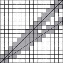
Figure 1. The pixelation of the angle $A\left(1,\frac{2}{3}\right)$ contains two holes.

Consider the pixelation of an angle $A\bigl{(}1,\frac{2}{3}\,\bigr{)}$ with vertex at the origin whose edges have slopes $\frac{2}{3}$ and $1$. Figure 1 shows that this pixelation is not contractible and in fact its first Betti number is $2$. These two “holes” won’t disappear at any resolution because all the pixelations of this angle are rescalings of each other.

Things can get a lot worse. For example, if $n$ is a positive integer and $S_{n}$ is the union of the two line segments connecting the origin to the points $(n,2n+1)$ and $(1,2)$, then for any ${\varepsilon}>0$ sufficiently small we have $b_{1}(\,P_{\varepsilon}(S_{n})\,)=2n$, while obviously $b_{1}(S_{n})=0$.

In [14] the second author solved the Main Problem in the special case when $S$ itself is a $PL$-set. The resulting algorithm is based on two key principles inspired by Morse theory.

Principle 1. Suppose that $S$ is the graph of a continuous piecewise $C^{2}$-function $f:[a,b]\to{\mathbb{R}}$, and the second order derivatives of $f$ are bounded. We fix a function ${\sigma}:(0,\infty)\rightarrow{\mathbb{Z}}_{>0}$, called the spread, such that

$$\lim_{{\varepsilon}\searrow 0}{\varepsilon}{\sigma}({\varepsilon})=0\;\;\mbox{and}\;\;\lim_{{\varepsilon}\searrow 0}{\varepsilon}{\sigma}({\varepsilon})^{2}=\infty \boldsymbol{\sigma}$$ ()

For any ${\varepsilon}>0$ every column of the pixelation $P_{\varepsilon}(S)$ is connected. For each ${\varepsilon}>0$ we obtain by linear interpolation a $PL$ function $\tau_{\varepsilon}$ (resp. $\beta_{\varepsilon}$) whose graph is produced by connecting with straight line segments the centers of the top (resp. bottom) pixels of every ${\sigma}({\varepsilon})$-th column of the pixelation of the graph of $f$; see Figure 2 where ${\sigma}=3$.

Figure 2. Linear interpolations with spread ${\sigma}=3$.

The result of the algorithm is the $PL$-region $S_{\varepsilon}$ between the graphs of $\beta_{\varepsilon}$ and $\tau_{\varepsilon}$. This is a very narrow two dimensional $PL$ set very close to the graph of $f$. Moreover, the condition ($\boldsymbol{\sigma}$) gurantees that the curvature of $S_{\varepsilon}$ resembles that of $S$.

An identical strategy works when $S$ is a set of the form

$$S=\bigl{\{}(x,y)\in{\mathbb{R}}^{2};\;\;x\in[a,b],\;;\beta(x)\leq y\leq\tau(x)\,\bigr{\}},$$

where $\beta,\tau:[a,b]\rightarrow{\mathbb{R}}$ are Hölder continuous, piecewise $C^{2}$-functions such that $\beta(x)\leq\tau(x)$, $\forall x\in[a,b]$.

We will refer to these two types of sets as elementary. Thus, the Main Problem has a solution for elementary sets.

Principle 2. Suppose that $S\subset{\mathbb{R}}^{2}$ is a generic $PL$-set, i.e., its $1$-dimensional skeleton does not contain vertical segments. Consider the linear map $h(x,y)=x$. The Morse theoretic properties of the restriction of $h$ to $P_{\varepsilon}(S)$ closely mimic the Morse theoretic properties of the restriction of $h$ to $S$ if ${\varepsilon}$ is sufficiently small. Here are the details.

For $x_{0}\in{\mathbb{R}}$ denote by ${\boldsymbol{n}}_{S}(x_{0})$ the number of connected components of the intersection of $S$ with the vertical line $\{x=x_{0}\}$ and denote by $\mathcal{J}_{S}$ the set of discontinuities of the function $x\mapsto{\boldsymbol{n}}_{S}(x)$. Then $\mathcal{J}_{S}$ is a finite subset of ${\mathbb{R}}$ and there exists $\gamma>0$ such that for any $r\in(0,\gamma)$ the set $S^{\prime}_{r}$ obtained from $S$ by removing the vertical strips $\{|x-j|<r\}$, $j\in\mathcal{J}_{S}$, is a disjoint union of elementary regions.

The set $\mathcal{J}_{S}$ is difficult to determine from a pixelation, but one can algorithmically produce a very small region containing it. Here is roughly the strategy.

For ${\varepsilon}>0$ and $x_{0}\in{\mathbb{R}}$ we denote by ${\boldsymbol{n}}_{S,{\varepsilon}}(x_{0})$ the number of connected components of the intersection of the vertical line $\{x=x_{0}\}$ with the pixelation $P_{\varepsilon}(S)$. We denote by $\mathcal{J}_{S,{\varepsilon}}$ the set of discontinuities of the function $x\mapsto{\boldsymbol{n}}_{S,{\varepsilon}}(x)$. The set $\mathcal{J}_{S,{\varepsilon}}$ is finite and one can prove the following remarkable robustness result.

($\boldsymbol{R}_{0}$) There exist $\hbar,\nu_{0}>0$ depending only on $S$, such that for ${\varepsilon}<\hbar$ we have

$$\operatorname{dist}(\mathcal{J}_{S},\mathcal{J}_{S,{\varepsilon}})<\nu_{0}{\varepsilon}.$$

Above, $\operatorname{dist}$ refers to the Hausdorff distance. We define the noise region to be the set

$$\mathcal{N}_{\varepsilon}:=\bigl{\{}x\in{\mathbb{R}};\;\;\operatorname{dist}(x,\mathcal{J}_{S,{\varepsilon}})\leq 2\nu{\varepsilon}\,\bigr{\}}.$$

For ${\varepsilon}$ sufficiently small, the noise region is a finite union of disjoint compact intervals

$$I_{j}({\varepsilon}),\;\;j=1,\dotsc,N:=\#\mathcal{J}_{S},$$

called noise intervals.

We denote by $P^{\prime}_{\varepsilon}(S)$ the closure of the set obtained from $P_{\varepsilon}(S)$ by removing the vertical strips $\{x\in I_{j}({\varepsilon})\}$, $j=1,\dotsc,N$. Each of the connected components of $P^{\prime}_{\varepsilon}(S)$ is the pixelation of an elementary set and as such it can be $PL$-approximated using Principle 1.

The approximation above the noise intervals, i.e., the intersection of $P_{\varepsilon}(S)$ with the above vertical strips is rather coarse. Every component of such a region is approximated by the smallest rectangle that contains it. Here by rectangle we mean a region of the form $[a,b]\times[c,d]$, $a\leq b$, $c\leq d$.

It turns out that the approximation $S_{\varepsilon}$ of $S$ obtained in this fashion from $P_{\varepsilon}(S)$ is very good in the following sense: the normal cycle of $S_{\varepsilon}$ converges in the sense of currents to the normal cycle of $S$. For a nice introduction to the subject of normal cycles we refer to [11]. A brief description of this concept can also be found on page 4.4 of this paper.

The goal of this paper is to extend the above program to the more general case of compact, semialgebraic subsets of ${\mathbb{R}}^{2}$. While Principle 1 extends with only little extra effort to the semi-algebraic case, Principle 2 requires a more delicate analysis. This requires that $S$ be a generic semialgebraic set in the sense that the restriction to $S$ of the linear function $h(x,y)=x$ be a stratified Morse function in the sense of Goresky-MacPherson; see [6, 13] or Section 1. In this case the set $\mathcal{J}_{S}$ can be alternatively described as the set of critical values of $h|_{S}$ corresponding to critical points whose Morse data in the sense of Goresky-MacPherson [6] are homotopically nontrivial.

We know that the stratified Morse function $h|_{S}$ is stable, [13]. Remarkably the function $h$ is also robust: some of the topological features of $h|_{S}$ are preserved if we slightly alter $S$ in a rather irregular way, by replacing it with one of its pixelations. More precisely we have the following counterpart of ($\boldsymbol{R}_{0}$).

($\boldsymbol{R}$) Suppose that $S\subset{\mathbb{R}}^{2}$ is a generic, compact semialgebraic set. Then there exist $\hbar>0$, $\nu_{0}>0$ and $\kappa_{0}\in(0,1]$, depending only on $S$ such that for ${\varepsilon}<\hbar$ we have

$$\operatorname{dist}(\mathcal{J}_{S},\mathcal{J}_{S,{\varepsilon}})<\nu_{0}{\varepsilon}^{\kappa_{0}}.$$

The main difference between ($\boldsymbol{R}$) and ($\boldsymbol{R}_{0}$) is the presence of the exponent $\kappa_{0}\in(0,1]$. This exponent takes into account the possibility that the $1$-dimensional skeleton of $S$ may have cusps such as $|y|^{p}=x^{q}$, $x\geq 0$, $\alpha=\frac{q}{p}\geq 1$. The higher the orders of contact $\alpha$ of such cusps, the lower the exponent $\kappa_{0}$. In fact $\kappa_{0}\leq\frac{1}{\alpha}$ for any order of contact $\alpha$. However, the choice $\kappa_{0}=\frac{1}{2}$ will work for many compact semialgebraic sets $S$.

The $PL$ approximation $S_{\varepsilon}$ of $S$ is obtained as before, using the two principles. To prove that the normal cycle of $S_{\varepsilon}$ converges in the sense of currents to the normal cycle of $S$ we rely on an approximation theorem of J. Fu, [7]. That theorem states that the convergence of the normal cycles is guaranteed once we prove two things.

• Uniform bounds for the perimeter and total curvature of $S_{\varepsilon}$.

• For almost any closed half-plane $H$ we have

  $$\lim_{{\varepsilon}\searrow 0}\chi\bigl{(}\,H\cap S_{\varepsilon}\,\bigr{)}=\chi\bigl{(}\,H\cap S\,\bigr{)},$$

  where $\chi$ denotes the Euler characteristic.

Of the above two facts, the second is by far the most delicate, and its proof takes up the bulk of this paper.

Let us say a few words about the organization of the paper. In Section 1 we introduce the terminology used throughout the paper. Principle 1 is proved in Section 2, while the robustness principle ($\boldsymbol{R}$) is proved in Section 3.

In Alorithm 4.3 of Section 4 we give an explicit and detailed description of the process that builds the approximation $S_{\varepsilon}$ starting from the pixelation $P_{\varepsilon}(S)$. This section contains the proof of the main result of the paper, Theorem 4.5, which states that the normal cycle of $S_{\varepsilon}$ converges to the normal cycle of $S$ as ${\varepsilon}\to 0$.

The paper concludes with two appendices. In Appendix A we collect a few basic facts of real algebraic geometry used throughout paper together with a few other technical results. In Appendix B we give a more formal description of the approximation algorithm in a way that makes it easily implementable on a computer.

Remark. After this work was completed we became aware of a recent work [3] where the authors investigate a similar problem in arbitrary dimensions. They used a completely different approach to produce an algorithm for approximating the curvature measures of a compact region $R$ in ${\mathbb{R}}^{n}$ . However the techniques used in [3] apply only to regions satisfying a so called positive $\mu$-reach condition. This condition prohibits the existence of cusp-like singularities in $R$. For example, the techniques in [3] are not apllicable to the region consisting of two tangent disks. $\hbox to0.0pt{$\sqcap$\hss}\sqcup$

Acknowledgment. We are very grateful to the anonymous referee for the many very useful and detailed comments, questions, suggestions and corrections which have helped us improve the quality of the paper.

1. Basic facts

We begin by recalling some basic notions introduced in [14].

Definition 1.1.

(a) Let ${\varepsilon}>0$. Then we define an ${\varepsilon}$-pixel to be the square in ${\mathbb{R}}^{2}$ of the form

$$S_{i,j}({\varepsilon})=[(i-1){\varepsilon},i{\varepsilon})]\times[(j-1){\varepsilon},j{\varepsilon})]\subset{\mathbb{R}}^{2},\;\;i,j\in{\mathbb{Z}}.$$

Its center is

$$c_{i,j}({\varepsilon}):=(i{\varepsilon},j{\varepsilon})-\left(\frac{{\varepsilon}}{2},\frac{{\varepsilon}}{2}\right).$$

(b) A union of finitely many ${\varepsilon}$-pixels is called an ${\varepsilon}$-pixelation. The variable ${\varepsilon}$ is called the resolution of the pixelation.

(c) For any compact subset $S\subset{\mathbb{R}}^{2}$ we define the ${\varepsilon}$-pixelation of $S$ to be the union of all the ${\varepsilon}$-pixels that intersect $S$. We denote the ${\varepsilon}$-pixelation of $S$ by $P_{\varepsilon}(S)$. The pixelation of a function $f$ is defined to be the pixelation of its graph $\Gamma(f)$. We will denote this pixelation by $P_{\varepsilon}(f)$. $\hbox to0.0pt{$\sqcap$\hss}\sqcup$

Definition 1.2.

Fix ${\varepsilon}>0$ and a compact set $S\subset{\mathbb{R}}^{2}$.

1. A point $a\in{\mathbb{R}}$ will be called ${\varepsilon}$-generic if $a\in{\mathbb{R}}\setminus{\varepsilon}{\mathbb{Z}}$. For such a point $a$ we denote by $I_{\varepsilon}(a)$ the interval of the form $(\,n{\varepsilon},(n+1){\varepsilon})$, $n\in{\mathbb{Z}}$ that contains $a$.

2. For $a<b$ we define the vertical strip

   $$\mathcal{S}_{a,b}:=(a,b)\times{\mathbb{R}}$$

   For every $k\in{\mathbb{Z}}$ we denote by $\mathcal{S}_{{\varepsilon},k}$ the vertical strip $\mathcal{S}_{k{\varepsilon},(k+1){\varepsilon}}$. For any ${\varepsilon}$-generic point $a\in{\mathbb{R}}$ we denote by $\mathcal{S}_{\varepsilon}(a)$ the strip $S_{{\varepsilon},k}$, $k:=\lfloor a/{\varepsilon}\rfloor$.

3. A column of $P_{\varepsilon}(S)$ is the intersection of $P_{\varepsilon}(S)$ with a vertical strip $\mathcal{S}_{{\varepsilon},k}$, $k\in{\mathbb{Z}}$. The connected components of a column are called stacks.

4. For every ${\varepsilon}$-generic $a\in{\mathbb{R}}$, we define the column of a pixelation $P_{\varepsilon}(S)$ over $a$ to be the set

   $$C_{\varepsilon}(S,a):=\mathcal{S}_{\varepsilon}(a)\cap P_{\varepsilon}(S).$$

   In other words, $C_{\varepsilon}(S,a)$ is the union of the pixels in $P_{\varepsilon}(S)$ which intersect the vertical line $\{x=a\}$. When $S$ is the graph of a function $f$, we will use the notation $C_{\varepsilon}(f,a)$ to denote the column over $a$ of the pixelation $P_{\varepsilon}(f)$.

$\hbox to0.0pt{$\sqcap$\hss}\sqcup$

We have the following result, [14, Thm. 2.2].

Theorem 1.3.

If $f:[a,b]\rightarrow{\mathbb{R}}$ is a continuous function, then for any ${\varepsilon}>0$ the columns of the ${\varepsilon}$-pixelation of the graph of $f$ consist of single stacks. $\hbox to0.0pt{$\sqcap$\hss}\sqcup$

In this paper we will be concerned with pixelations of generic planar semialgebraic sets, where the genericity has a very precise meaning. To describe it we need to introduce some terminology from stratified Morse theory, [6, 13].

For any subset $X\subset{\mathbb{R}}^{2}$ we denote by $\operatorname{\boldsymbol{cl}}(X)$ its closure and by $\partial_{\mathrm{top}}X$ its topological boundary,

$$\partial_{\mathrm{top}}(X):=\operatorname{\boldsymbol{cl}}(X)\setminus X.$$

We define a good stratification of a compact semialgebraic set $S\subset{\mathbb{R}}^{2}$ to be an increasing filtration

$$\mathcal{F}:\;\;F^{(0)}\subset F^{(1)}\subset F^{(2)}=S$$

satisfying the following properties.

• Each of the sets $F^{(i)}$, $i=0,1,2$ is closed.

• $\dim F^{(i)}\leq i$, $i=0,1,2$. In particular $F^{(0)}$ is a finite collection of points called the vertices of the good stratification.

• The connected components of $F^{(1)}\setminus F^{(0)}$ are open real analytic arcs, i.e., images of injective real analytic maps $(0,1)\rightarrow{\mathbb{R}}^{2}$. We will refer to these components as the arcs or the edges of the stratification.

• The connected components of $F^{(2)}\setminus F^{(1)}$ are open subsets of ${\mathbb{R}}^{2}$. They are called the faces of the stratification.

• $$\partial_{\mathrm{top}}\bigl{(}\,F^{(2)}\setminus F^{(1)}\,\bigr{)}\subset F^{(1)},\;\;\partial_{\mathrm{top}}\bigl{(}F^{(1)}\setminus F^{(0)}\,\bigr{)}\subset F^{(0)}.$$

Definition 1.4.

Suppose that $v$ is a vertex of a good stratification of a compact semialgebraic set $S\subset{\mathbb{R}}^{2}$. The tangent cone $C_{\infty}(v,S)$ to $S$ at $v$ consists of finitely many one-dimensional subspaces of ${\mathbb{R}}^{2}$. More precisely, a line $L_{\infty}\subset{\mathbb{R}}^{2}$ belongs to the tangent cone $C(v,S)$ iff there exists an arc $A$ of the stratification of $S$ with the following properties.

• $v\in\operatorname{\boldsymbol{cl}}(A)$.

• There exists a sequence of points $v_{n}\in A$ such that as $n\rightarrow\infty$ we have $v_{n}\rightarrow v$ and the tangent spaces $T_{v_{n}}A$ converge to $L_{\infty}$.

$\hbox to0.0pt{$\sqcap$\hss}\sqcup$

Suppose that $S\subset{\mathbb{R}}^{2}$ is a compact semialgebraic set equipped with a good stratification $\mathcal{F}$, and $f:{\mathbb{R}}^{2}\rightarrow{\mathbb{R}}$. A point $p\in S$ is said to be a critical point of the restriction $f|_{S}$ if either $p$ is a vertex, or $p$ is the critical point of the restriction of $f$ to an arc or to a face. The critical point $p$ is said to be nondegerate if it satisfies one of the following conditions.

• The point $p$ is a vertex and for any $L_{\infty}\in C_{\infty}(p,S)$, the differential of $f$ at $p$ does not vanish along $L_{\infty}$.

• The point $p$ belongs to an arc $A$ of the stratification and as such it is a nondegenerate point of $f|_{A}$.

• The point $p$ belongs to a face $F$ of the stratification and as such it is a nondegenerate point of $f|_{F}$.

A function $f:{\mathbb{R}}^{2}\rightarrow{\mathbb{R}}$ is said to be a a stratified Morse function with respect to the semialgebaric set $S$ equipped with the good stratification $\mathcal{F}$ if all its critical points are nondegenerate, and no two critical points lie on the same level set of $f$.

A compact semialgebraic set $S\subset{\mathbb{R}}^{2}$ is called generic if it admits a good stratification $\mathcal{F}$ such that projection onto the $x$-axis $(x,y)\mapsto x$ is a stratified Morse function with respect to $(S,\mathcal{F})$. Denote this projection by $\boldsymbol{h}$.

Observe that if $\mathcal{F}$ is a good stratification of a compact semialgebraic set $S\subset{\mathbb{R}}^{2}$, then $p$ is a critical point of $\boldsymbol{h}$ relative to $(S,\mathcal{F})$ if either $p$ is a vertex of the stratification, or $p$ is a point on an arc of $\mathcal{F}$ where the the tangent space is vertical. At such a point the arc is locally on one side of that vertical tangent.

Figure 3. The curve on the right is generic, while the curve on the left is not.

In Figure 3 we have depicted two one-dimensional planar semi algebraic curves (arcs of circles). The marked points are critical points of $\boldsymbol{h}$. The point $A$ on the left-hand side curve is a degenerate critical point because the condition ($\boldsymbol{C}_{0}$) is violated: the vertical line is tangent to the curve at that point.

In the left-hand side of Figure 4 we have depicted further examples of pathologies prohibited by the genericity condition. (The pathologies involve the points with vertical tangencies.) The right-hand side depicts generic sets obtained by small perturbations from the nongeneric sets in the left-hand side.

Figure 4. The curves on the left-hand side are nongeneric. They become generic after a small perturbation.

2. Approximations of elementary sets

In this section we study the pixelations of simple two dimensional sets.

Definition 2.1.

Fix ${\varepsilon}>0$ and a compact set $S$.

1. An ${\varepsilon}$-profile of $S$ is a set $\Pi_{\varepsilon}$ of points in the plane with the following properties.

   1. Each point in $\Pi_{\varepsilon}$ is the center of an ${\varepsilon}$-pixel that intersects $S$.

   2. Every column of $P_{\varepsilon}(S)$ contains precisely one point of $\Pi_{\varepsilon}$.

2. The top/bottom ${\varepsilon}$-profile is the profile consisting of the centers of the highest/lowest pixels in each column of $P_{\varepsilon}(S)$.

3. An ${\varepsilon}$-sample of $S$ is a subset of an ${\varepsilon}$-profile. An upper/lower ${\varepsilon}$-sample of $S$ is an ${\varepsilon}$-sample of the upper/lower ${\varepsilon}$-profile of $S$.

4. Two ${\varepsilon}$-samples are called compatible if they have the same projections on the $x$-axis.

$\hbox to0.0pt{$\sqcap$\hss}\sqcup$

Definition 2.2.

Suppose $p_{1},\dotsc,p_{N}$ is a finite sequence of points in ${\mathbb{R}}^{2}$. (The points need not be distinct). We denote by

$$\langle p_{1},p_{2},\dotsc,p_{n}\rangle$$

the $PL$ curve defined as the union of the straight line segments $[p_{1},p_{2}],\dotsc,[p_{n-1},p_{n}]$. $\hbox to0.0pt{$\sqcap$\hss}\sqcup$

Observe that each ${\varepsilon}$-profile $\Pi_{\varepsilon}$ of a set is equipped with a linear order $\preceq$. More precisely, if $p_{1},p_{2}$ are points in $\Pi_{\varepsilon}$, then

$$p_{1}\preceq p_{2}\Longleftrightarrow x(p_{1})\leq x(p_{2}),$$

where $x:{\mathbb{R}}^{2}\rightarrow{\mathbb{R}}$ denotes the projection $(x,y)\mapsto x$. In particular, this shows that any ${\varepsilon}$-sample of $S$ carries a natural total order.

Definition 2.3.

If $\Xi$ is an ${\varepsilon}$-sample of $S$, then the $PL$-interpolation determined by the sample $\Xi$ is the continuous, piecewise linear function $L=L_{\Xi}$ obtained as follows.

• Arrange the points in $\Xi$ in increasing order, with respect to the above total order,

  $$V=\{\xi_{0}\prec\xi_{1}\prec\xi_{2}\prec\cdots\prec\xi_{n}\},\;\;n+1=|\Xi|.$$

• The graph of $L_{\Xi}$ is the $PL$-curve $\langle\xi_{0},\xi_{1},\dotsc,\xi_{n}\rangle$.

$\hbox to0.0pt{$\sqcap$\hss}\sqcup$

In applications, the sample sets $\Xi$ will be chosen to satisfy certain regularity.

Definition 2.4.

1. A spread function is a nonincreasing function ${\sigma}:(0,\infty)\to{\mathbb{Z}}_{>0}$ with the following properties.

   $$\lim_{{\varepsilon}\searrow 0}\sigma({\varepsilon})=\infty,$$ (2.1a)

   $$\lim_{{\varepsilon}\searrow 0}{\varepsilon}\sigma({\varepsilon})=0.$$ (2.1b)

2. If $\sigma$ is a positive integer and $\Pi_{\varepsilon}$ is an ${\varepsilon}$-profile, then an ${\varepsilon}$-sample with spread $\sigma$ is a subset

   $$\Xi=\{\xi_{0}\prec\cdots\prec\xi_{n}\}\subset\Pi_{\varepsilon}(S)$$

   such that the following hold.

   • The points $\xi_{0}$ and $\xi_{n}$ are the left and rightmost points in the profile, i.e., for each $p\in\Pi_{\varepsilon}$, $x(\xi_{0})\leq x(p)\leq x(\xi_{n})$.

   • $$\frac{1}{2}{\varepsilon}\sigma({\varepsilon}\leq|x(\xi_{k})-x(\xi_{k-1})|\leq{\varepsilon}\sigma({\varepsilon}),\;\;\forall k=1,\dotsc,n.$$

$\hbox to0.0pt{$\sqcap$\hss}\sqcup$

Definition 2.5.

A subset $S\subset{\mathbb{R}}^{2}$ is said to be elementary over the interval $[a,b]$ if it can be defined as

$$S=S(\beta,\tau):=\bigl{\{}\,(x,y):\;\;x\in[a,b],\beta(x)\leq y\leq\tau(x)\,\bigr{\}},$$

where $\beta,\tau:[a,b]\rightarrow{\mathbb{R}}$ are continuous semialgebraic functions such that $\beta(x)\leq\tau(x)$, $\forall x\in[a,b]$.

The function $\beta$ is called the bottom of $S$ while $\tau$ is called the top of $S$. If

$$\beta(x)<\tau(x),\;\;\forall x\in(a,b),$$ (2.2)

then the elementary set is said to be nondegenerate. If

$$\beta(x)=\tau(x),\;\;\forall x\in[a,b],$$ (2.3)

then the set $S$ is called degenerate. The elementary set is called mixed if both sets

$$\bigl{\{}x\in(a,b);\;\;\tau(x)-\beta(x)>0\,\bigr{\}}\;\;\mbox{and}\;\;\bigl{\{}x\in(a,b);\;\;\tau(x)-\beta(x)=0\,\bigr{\}}$$

are nonempty. $\hbox to0.0pt{$\sqcap$\hss}\sqcup$

Observe that an elementary set $S(\beta,\tau)$ over the compact interval $[a,b]$ admits good partitions, i.e., partitions

$$a=c_{0}<c_{1}<c_{1}<\cdots<c_{n}=b,\;\;n\geq 2$$

such that each of the elementary sets $[c_{i-1},c_{i}]\times{\mathbb{R}}\cap S(\beta,\tau)$ is either degenerate or nondegenerate. The good partition with minimal $n$ is called the minimal good partition; see Figure 5.

Figure 5. The minimal good partition of a mixed elementary set.

In the remainder of this section $S$ will indicate an elementary set. We first note that like the pixelation of a function, each column of $P_{\varepsilon}(S)$ consists of a single stack, i.e., a single connected component.

Proposition 2.6.

If $S=S(\beta,\tau)$ is an elementary set over a compact interval $[a,b]$, then for every $x\in[a,b]\setminus{\varepsilon}{\mathbb{Z}}$, the column $C_{\varepsilon}(S,x)$ consists of exactly one stack.

Proof.

Fix an ${\varepsilon}$-generic $x\in[a,b]$. By Theorem 1.3 the columns $C_{\varepsilon}(\beta,x)$ and $C_{\varepsilon}(\tau,x)$ consist of single stacks. If these two columns intersect, then the conclusion is obvious. If they do not intersect, then any pixel in the strip $S_{\varepsilon}(x)$ situated below the stack $C_{\varepsilon}(\tau,x)$ and above the stack $C_{\varepsilon}(\beta,x)$ is a pixel of $P_{\varepsilon}(S)$. This proves that the column $C_{\varepsilon}(S,x)$ consists of a single stack. $\hbox to0.0pt{$\sqcap$\hss}\sqcup$

Definition 2.7.

Fix ${\varepsilon}>0$ and an elementary set $S=S(\beta,\tau)$. Suppose that $\Xi^{\pm}_{\varepsilon}$ are compatible upper/lower samples of $S$

$$\Xi^{\pm}_{\varepsilon}=\{\xi_{0}^{\pm}\prec\xi_{1}^{\pm}\prec\cdots\prec\xi_{n}^{\pm}\}.$$

The $PL$-approximation of $S$ determined by these two samples is the compact $PL$-set bounded by the closed $PL$-curve

$$\langle\xi_{0}^{-},\xi_{1}^{-},\dotsc,\xi_{n}^{-},\xi_{n}^{+},\xi_{n-1}^{+},\dotsc,\xi_{0}^{+},\xi_{0}^{-}\rangle.$$

$\hbox to0.0pt{$\sqcap$\hss}\sqcup$

The total curvature of a $C^{1}$-immersion $\gamma:[a,b]\rightarrow{\mathbb{R}}^{2}$ which is $C^{2}$ on $(a,b)$ is defined as follows. We set

$${\boldsymbol{v}}(t):=\frac{1}{|\dot{\gamma}(t)|}\dot{\gamma(t)},\;\;\kappa(t):=|\dot{{\boldsymbol{v}}}(t)|.$$

The scalar $\kappa(t)$ is called the curvature of $\gamma$ at the point $\gamma(t)$. We define the total curvature of $\gamma$ to be

$$K(\gamma):=\int_{a}^{b}\kappa(t)\,dt.$$

Suppose now that $\gamma:[a,b]\rightarrow{\mathbb{R}}^{2}$ is a continuous and piecewise $C^{2}$-immersion, i.e., there exists a finite subset $\{t_{0},\dotsc,t_{\nu}\}\subset[a,b]$, such that

$$a=t_{0}<t_{1}<\cdots<t_{\nu-1}<t_{\nu}=b,$$

the restriction $\gamma_{i}:=\gamma|_{[t_{i-1},t_{i}]}$ is a $C^{1}$ immersion, and the restriction of $\gamma$ to the open interval to $(t_{i-1},t_{i})$ is $C^{2}$, for any $i=1,\dotsc,\nu$. The curvature of $\gamma$ at a jump point $\gamma(t_{i})$ is the quantity

$$\kappa(t_{i}):=\lim_{{\varepsilon}\searrow 0}\operatorname{dist}_{S^{1}}\bigl{(}\,{\boldsymbol{v}}(t_{i}+{\varepsilon})\,,\,{\boldsymbol{v}}(t_{i}-{\varepsilon})\,\bigr{)},$$

where $\operatorname{dist}_{S^{1}}(p,q)\in[0,\pi]$ denotes the geodesic distance between two points $p,q$ on the unit circle. We define the total curvature of $\gamma$ to be

$$\begin{split}K(\gamma)&:=\sum_{i=1}^{\nu}K(\gamma_{i})+\sum_{i=1}^{\nu-1}\kappa(t_{i})\\ &+\begin{cases}0,&\gamma(b)\neq\gamma(a),\\ &\\ \operatorname{dist}_{S_{1}}\bigl{(}\,{\boldsymbol{v}}(b^{-}),{\boldsymbol{v}}(a^{+}\,\bigr{)},&\gamma(b)=\gamma(a).\end{cases}\end{split}$$

For more details we refer to [10] and [11, §2.2].

We define a semialgebraic arc to be the image of a continuous, injective semialgebraic map

$${\varphi}:[a,b]\rightarrow{\mathbb{R}}^{2}.$$

Suppose that ${\varphi}:[a,b]\rightarrow{\mathbb{R}}^{2}$ is a continuous, injective, semialgebraic map whose image is the semialgebraic arc $\boldsymbol{C}$. Set $A:={\varphi}(a)$ and $B:={\varphi}(b)$ so that $\boldsymbol{C}$ connects $A$ to $B$. The semialgebraic map ${\varphi}$ is piecewise $C^{2}$ and has a total curvature which a priori could be infinite.

Lemma 2.8.

The total curvature of a semialgebraic arc $C\subset{\mathbb{R}}^{2}$ is finite.

Proof.

The arc $C$ has finitely many singularities and their complement is a finite union of oriented, bounded, semialgebraic, $C^{1}$-arcs. If $C_{i}$ is such an arc, then its total curvature is the length of the oriented Gauss path $\Gamma_{i}:C_{i}\to S^{1}$, where $\Gamma_{i}(p)$ is the unique unit vector in $T_{p}C_{i}$ determined by the orientation of $C_{i}$. Since the Gauss map is semialgebraic and $C_{i}$ has finite length we deduce that the length of $\Gamma_{i}$ is finite. The contributions to the total curvatures of the finitely many singular points of $C$ are all finite. $\hbox to0.0pt{$\sqcap$\hss}\sqcup$

Suppose that $\boldsymbol{C}$ is a semialgebraic arc defined by the the continuous, semialgebraic injection ${\varphi}:[a,b]\to{\mathbb{R}}^{2}$. An ordered sampling of $\boldsymbol{C}$ is an ordered collection of points

$${\mathcal{P}}:=\bigl{\{}P_{1},\dotsc,P_{n}\,\bigr{\}}\subset\boldsymbol{C},$$

such that the collection

$${\varphi}^{-1}({\mathcal{P}}):=\bigl{\{}t_{1}={\varphi}^{-1}(P_{1}),\dotsc,t_{n}:={\varphi}^{-1}(P_{n})\bigr{\}}\subset[a,b]$$

satisfies

$$t_{1}<t_{2}<\cdots<t_{n}.$$

The mesh of the ordered sampling ${\mathcal{P}}$ is the positive number

$$\|{\mathcal{P}}\|:=\max\bigl{\{}\,\operatorname{dist}(A,P_{1}),\operatorname{dist}(P_{1},P_{2}),\dotsc,\operatorname{dist}(P_{n-1},P_{n}),\operatorname{dist}(P_{n},B)\,\bigr{\}}.$$

We denote by $\boldsymbol{C}({\mathcal{P}})$ the $PL$-curve $\langle P_{1},\dotsc,P_{n}\rangle$.

A result of J. Milnor, [10, Thm.2.2], shows that the total curvature of a $C^{2}$-curve can be approximated by the total curvature of inscribed polygons. The next result, whose proof is delegated to Appendix A, shows that if the curve is semialgebraic, then the $C^{2}$ requirement is not necessary.

Proposition 2.9.

Suppose that $\boldsymbol{C}$ is a semialgebraic arc and for every ${\varepsilon}>0$ we are given an ordered sampling ${\mathcal{P}}_{\varepsilon}$ of $\boldsymbol{C}$. Denote by $L$ (resp. $K$) the length (resp. total curvature) of $\boldsymbol{C}$ and by $L_{\varepsilon}$ (resp. $K_{\varepsilon}$) the length (resp. total curvature) of $\boldsymbol{C}({\mathcal{P}}_{\varepsilon})$. If

$$\lim_{{\varepsilon}\searrow 0}\|{\mathcal{P}}_{\varepsilon}\|=0,$$

then

$$\lim_{{\varepsilon}\searrow 0}L_{\varepsilon}=L\;\;\mbox{and}\;\;\lim_{{\varepsilon}\searrow 0}K_{\varepsilon}=K.$$

$\hbox to0.0pt{$\sqcap$\hss}\sqcup$

Theorem 2.10.

Suppose that $h:[a,b]\rightarrow{\mathbb{R}}$ is a continuous semialgebraic function and ${\varepsilon}\mapsto{\sigma}({\varepsilon})$ is a spread function satisfying the additional condition

$$\lim_{{\varepsilon}\searrow 0}{\varepsilon}{\sigma}({\varepsilon})^{2}=\infty.$$ (2.4)

For every ${\varepsilon}>0$ we choose an ${\varepsilon}$-sample $\Xi_{\varepsilon}$ with spread ${\sigma}({\varepsilon})$ of the graph $\Gamma$ of $h$. Denote by $\boldsymbol{C}_{\varepsilon}$ the graph of the $PL$-function $L_{\Xi_{\varepsilon}}$ described in Definition 2.3. Then, as ${\varepsilon}\searrow 0$ we have

$${\rm length}\,(\boldsymbol{C}_{\varepsilon})\rightarrow{\rm length}\,(\Gamma)\;\;\mbox{and}\;\;K(\boldsymbol{C}_{\varepsilon})\rightarrow K(\Gamma).$$

Proof.

We use a simple strategy. More precisely for every ${\varepsilon}>0$ we construct an ordered sampling ${\mathcal{P}}_{\varepsilon}$ of $\Gamma$ such that

$$\lim_{{\varepsilon}\searrow 0}\|{\mathcal{P}}_{\varepsilon}\|=0,$$ (2.5)

and if $\Gamma_{\varepsilon}$ denotes the $PL$-curve $\Gamma({\mathcal{P}}_{\varepsilon})$ determined by the ordered sampling ${\mathcal{P}}_{\varepsilon}$, then as ${\varepsilon}\searrow 0$ we have

$${\rm length}\,(\boldsymbol{C}_{\varepsilon})={\rm length}\,(\Gamma_{\varepsilon})+O\left(\frac{1}{{\sigma}({\varepsilon})}\right),$$ (2.6a)

$$K(\boldsymbol{C}_{\varepsilon})=K(\Gamma_{\varepsilon})+O\left(\frac{1}{{\varepsilon}{\sigma}({\varepsilon})^{2}}\right).$$ (2.6b)

The desired conclusions will then follow from Proposition 2.9.

Suppose that $\Xi_{\varepsilon}$ consists of the points $Q_{0}^{\varepsilon},Q_{1}^{\varepsilon},\dotsc,Q_{n({\varepsilon})}^{\varepsilon}$ arranged in the increasing order defined by their $x$-coordinates. Observe that since $\Xi_{\varepsilon}$ has spread ${\sigma}({\varepsilon})$ then

$$n({\varepsilon})<\frac{2(b-a)}{{\varepsilon}{\sigma}({\varepsilon})}.$$ (2.7)

Each of the points of $\Xi_{\varepsilon}$ is the center of a pixel that touches $\Gamma$. Thus, for any $k=0,1,\dotsc,n({\varepsilon})$ there exists a point $P_{k}^{\varepsilon}\in\Gamma$ that lies in the same pixel as $Q_{k}^{\varepsilon}$. We obtain in this fashion an ordered sampling

$${\mathcal{P}}_{\varepsilon}=\bigl{\{}P_{0}^{\varepsilon},P_{1}^{\varepsilon},\dotsc,P_{n({\varepsilon})}^{\varepsilon}\,\bigr{\}}$$

of $\Gamma$. The function $h$ is continuous and semialgebraic and thus it is Hölder continuous with some Hölder exponent $\alpha\in(0,1]$. This proves that

$$\|{\mathcal{P}}_{\varepsilon}\|=O\bigl{(}\;\bigl{(}\,{\varepsilon}{\sigma}({\varepsilon})\;\bigr{)}^{\alpha}\,\bigr{)}.$$

The condition (2.5) now follows from the property (2.1b) of a spread function.

From the choice of the points $P_{k}^{\varepsilon}$ we deduce that for any $k=1,\dotsc,n({\varepsilon})$ we have

$$-{\varepsilon}\sqrt{2}<\operatorname{dist}(P_{k-1}^{\varepsilon},P_{k}^{\varepsilon})-\operatorname{dist}(Q_{k-1}^{\varepsilon},Q_{k}^{\varepsilon})<{\varepsilon}\sqrt{2}$$

so that by summing over $k$ we deduce

$$-\frac{2\sqrt{2}(b-a)}{{\sigma}({\varepsilon})}\stackrel{{\scriptstyle(\ref{eq: subdivisions})}}{{\leq}}-n({\varepsilon}){\varepsilon}\sqrt{2}<{\rm length}\,(\Gamma_{\varepsilon})-{\rm length}\,(\boldsymbol{C}_{\varepsilon})\leq n({\varepsilon}){\varepsilon}\sqrt{2}\stackrel{{\scriptstyle(\ref{eq: subdivisions})}}{{\leq}}\frac{2\sqrt{2}(b-a)}{{\sigma}({\varepsilon})}.$$

The equality (2.6a) now follows from the property (2.1a) of a spread function.

Now we turn to the total curvature. For any point $P\in{\mathbb{R}}^{2}$ we denote by $x(P)$, $y(P)$ its coordinates. For $k=1,\dotsc,n({\varepsilon})$ we denote by $m_{k}^{\varepsilon}$ the slope of the segment $[P_{k-1}^{\varepsilon},P_{k}^{\varepsilon}]$ and by $\bar{m}_{k}^{\varepsilon}$ the slope of the segment $[Q_{k-1}^{\varepsilon},Q_{k}^{\varepsilon}]$,

$$m_{k}^{\varepsilon}=\frac{y(P_{k}^{\varepsilon})-y(P_{k-1}^{\varepsilon})}{x(P_{k}^{\varepsilon})-x(P_{k-1}^{\varepsilon})},\;\;\bar{m}_{k}^{\varepsilon}=\frac{y(Q_{k}^{\varepsilon})-y(Q_{k-1}^{\varepsilon})}{x(Q_{k}^{\varepsilon})-x(Q_{k-1}^{\varepsilon})}.$$

Note that for any ${\varepsilon}>0$ and any $k=1,\dotsc,n({\varepsilon})$ we have from the definition of a spread that

$$\frac{1}{2}{\varepsilon}{\sigma}({\varepsilon})\leq x\bigl{(}\,Q_{k}^{\varepsilon}\,\bigr{)}-x\bigl{(}\,Q_{k-1}^{\varepsilon}\,\bigr{)}\,\leq{\varepsilon}{\sigma}({\varepsilon}).$$

Furthermore we have shown that

$$\operatorname{dist}(Q_{k}^{\varepsilon},P_{k}^{\varepsilon})\leq{\varepsilon}\sqrt{2}.$$

These two inequalities imply that

$$|m_{k}^{\varepsilon}-\bar{m}_{k}^{\varepsilon}|=O\left(\frac{1}{\sigma({\varepsilon})}\right)$$

There exist $\theta_{k}^{\varepsilon},\bar{\theta}^{\varepsilon}_{k}\in(-\frac{\pi}{2},\frac{\pi}{2})$ such that

$$m_{k}^{\varepsilon}=\tan\theta^{\varepsilon}_{k},\;\;\bar{m}^{\varepsilon}_{k}=\tan\bar{\theta}^{\varepsilon}_{k}.$$

The formula for the tangent of a difference of angles implies that

$$\theta_{k}^{\varepsilon}-\bar{\theta}_{k}^{\varepsilon}=\arctan\left(\frac{m_{k}^{\varepsilon}-\bar{m}_{k}^{\varepsilon}}{1+m_{k}^{\varepsilon}\bar{m}_{k}^{\varepsilon}}\right).$$

Using the above equality and the fact that $|m_{k}^{\varepsilon}-\bar{m}_{k}^{\varepsilon}|=O\left(\frac{1}{\sigma({\varepsilon})}\right)$, we see that there exists a positive constant $C$ independent of ${\varepsilon}$ such that

$$|\theta_{k}^{\varepsilon}-\bar{\theta}_{k}^{\varepsilon}|\leq\frac{C}{\sigma({\varepsilon})}$$

and therefore

$$\bigl{|}\,K(\Gamma_{\varepsilon})-K(\boldsymbol{C}_{\varepsilon})\,\bigr{|}\leq\frac{Cn({\varepsilon})}{{\sigma}({\varepsilon})}\stackrel{{\scriptstyle(\ref{eq: subdivisions})}}{{\leq}}\frac{C(b-a)}{{\varepsilon}{\sigma}({\varepsilon})^{2}}.$$

The equality (2.6b) now follows from (2.4). $\hbox to0.0pt{$\sqcap$\hss}\sqcup$

Corollary 2.11.

Let $S(\beta,\tau)$ be an elementary set. Fix a spread function ${\sigma}({\varepsilon})$ satisfying the condition (2.4). For each ${\varepsilon}$ we choose compatible ${\varepsilon}$-upper/lower profiles $\Xi^{\pm}_{\varepsilon}$ of $S$ with spread ${\sigma}({\varepsilon})$. We denote by ${S}_{\varepsilon}$ the $PL$ approximation of ${S}$ defined by these samples. Then

$$\lim_{{\varepsilon}\searrow 0}{\rm length}\,(\partial S_{\varepsilon})={\rm length}\,(\partial S),$$ (2.8a)

$$\lim_{{\varepsilon}\searrow 0}K(\partial S_{\varepsilon})=K(\partial S).$$ (2.8b)

Proof.

The semialgebraic functions $\beta$ and $\tau$ are differentiable outside a finite subset of $(a,b)$ and the limits

$$\beta^{\prime}(a):=\lim_{x\searrow a}\beta^{\prime}(x),\;\;\tau^{\prime}(a):=\lim_{x\searrow a}\tau^{\prime}(x),$$

$$\beta^{\prime}(b):=\lim_{x\nearrow b}\beta^{\prime}(x),\;\;\tau^{\prime}(b):=\lim_{x\nearrow b}\tau^{\prime}(x)$$

exist in $[-\infty,\infty]$. Let

$$\Xi^{\pm}_{\varepsilon}=\bigl{\{}\xi_{0}^{\pm}\prec\xi_{1}^{\pm}\prec\cdots\prec\xi_{n({\varepsilon})}^{\pm}\,\bigr{\}},\;\;\xi_{k}^{\pm}=:(x_{k}^{\pm},y_{k}^{\pm}).$$

The compatibility condition implies that

$$x_{k}^{-}=x_{k}^{+}=:x_{k},\;\;y_{k}^{-}\leq y_{k}^{+},\;\;\forall k=0,1,\dotsc,n.$$

Let $\beta_{\varepsilon}$ be the PL function whose graph is $L_{\Xi_{\varepsilon}^{-}}$ and $\tau_{\varepsilon}$ be the PL function whose graph is $L_{\Xi_{\varepsilon}^{+}}$. Let $m_{i}^{\beta}({\varepsilon})$ indicate the slope of the $i$-th line segment of the graph of $\beta_{\varepsilon}$ and similarly let $m_{i}^{\tau}({\varepsilon})$ indicate the slope of the $i$-th line segment of the graph of $\tau_{\varepsilon}$. We have

$${\rm length}(\partial S_{\varepsilon})={\rm length}\,(\Gamma_{\beta_{\varepsilon}})+{\rm length}\,(\Gamma_{\tau_{\varepsilon}})+\operatorname{dist}(\xi_{0}^{-},\xi_{0}^{+})+\operatorname{dist}(\xi_{n({\varepsilon})}^{-},\xi_{n({\varepsilon})}^{+}\,).$$

Theorem 2.10 implies that as ${\varepsilon}\searrow 0$ we have

$${\rm length}\,(\Gamma_{\beta_{\varepsilon}})\rightarrow{\rm length}\,(\Gamma_{\beta}),\;\;{\rm length}\,(\Gamma_{\tau_{\varepsilon}})\rightarrow{\rm length}\,(\Gamma_{\tau}).$$

Moreover, as ${\varepsilon}\searrow 0$ we have

$$\operatorname{dist}(\xi_{0}^{-},\xi_{0}^{+})\rightarrow\operatorname{dist}(\beta(a),\tau(a)\,),\;\;\operatorname{dist}(\xi_{n({\varepsilon})}^{-},\xi_{n({\varepsilon})}^{+}\,)\rightarrow\operatorname{dist}(\,\beta(b),\tau(b)\,).$$

This proves (2.8a).

Similarly

$$\begin{split}K(\partial S_{\varepsilon})&=|\pi-\arctan(m_{1}^{\beta}({\varepsilon})\,)|\\ &+\sum_{i=2}^{n}|\arctan(m_{i}^{\beta}({\varepsilon})\,)-\arctan(m_{i-1}^{\beta}({\varepsilon})\,)|\\ &+|\arctan(m_{n}^{\beta}({\varepsilon}))-\pi|+|\pi-\arctan(m_{1}^{\tau})|\\ &+\sum_{i=2}^{n}|\arctan(m_{i}^{\tau}({\varepsilon})\,)-\arctan(m_{i-1}^{\tau}({\varepsilon})\,)|\\ &+|\arctan(m_{n}^{\tau}({\varepsilon})\,)-\pi|\end{split}$$

which can be rewritten as

$$\begin{split}K(\partial S_{\varepsilon})&=|\pi-\arctan(m_{1}^{\beta}({\varepsilon})\,)|+|\arctan(m_{n}^{\beta}({\varepsilon})\,)-\pi|\\ &+|\pi-\arctan(m_{1}^{\tau}({\varepsilon})\,)|+|\arctan(m_{n}^{\tau}({\varepsilon})\,)-\pi|\\ &+K(\beta_{\varepsilon})+K(\tau_{\varepsilon})\end{split}$$ (2.9)

Theorem 2.10 implies

$$\lim_{{\varepsilon}\searrow 0}K(\beta_{\varepsilon})=K(\beta)\;\;\mbox{and}\;\;\lim_{{\varepsilon}\searrow 0}K(\tau_{\varepsilon})=K(\tau).$$ (2.10)

Now note that each line segment is defined by connecting two points in the pixelation of $\beta$ or $\tau$ over an interval of at most ${\varepsilon}\sigma({\varepsilon})$. As ${\varepsilon}\to 0$ we have

$$\begin{split}\lim_{{\varepsilon}\searrow 0}m_{1}^{\beta}({\varepsilon})=\beta^{\prime}(a),\;\;\lim_{{\varepsilon}\searrow 0}m_{n}^{\beta}({\varepsilon})=\beta^{\prime}(b),\\ \lim_{{\varepsilon}\searrow 0}m_{1}^{\tau}({\varepsilon})=\tau^{\prime}(a),\;\;\lim_{{\varepsilon}\searrow 0}m_{n}^{\tau}({\varepsilon})=\beta^{\prime}(b).\end{split}$$ (2.11)

Combining (2.9), (2.10), (2.11) we find that

$$\begin{split}\lim_{{\varepsilon}\searrow 0}K(\partial S_{\varepsilon})&=|\pi-\arctan(\beta^{\prime}(a))|+|\arctan(\beta^{\prime}(b))-\pi|\\ &+|\pi-\arctan(\tau^{\prime}(a))|+|\arctan(\tau^{\prime}(b))-\pi|\\ &+K(\beta)+K(\tau).\end{split}$$ (2.12)

Note that $|\pi-\arctan(\beta^{\prime}(a))|$ is the value of the angle between the vertical line $x=a$ and the tangent line to the graph of $\beta$ at $(a,\beta(a))$. Similarly each other difference on the right hand side of (2.12) corresponds to an angle at one of the corners of $\partial S$. Therefore the right hand side of the (2.12) is equal to the $K(\partial S)$, so the corollary holds. $\hbox to0.0pt{$\sqcap$\hss}\sqcup$

3. Separation results

In the previous section we have dealt only with the elementary regions and we have investigated mainly geometric properties of these regions and their pixelation. In this section we turn our attention to the relationship between the topologies of a semialgebraic set and those of its pixelations.

Surprisingly, this is a nontrivial matter. As shown in the introduction the homotopy type of a planar set may be quite different from those of its pixelations and this can happen even for a simple $PL$ set. The next result provides a first ray of hope. For any compact set $X\subset{\mathbb{R}}^{2}$ we denote by $\mathcal{C}(X)$ the set of connected components of $X$.

Proposition 3.1.

Let $S\subset{\mathbb{R}}^{2}$ be a compact semialgebraic set. Then for sufficiently small ${\varepsilon}$, the number of connected components of $P_{\varepsilon}(S)$ agrees with the number of connected components of $S$.

Proof.

We have a natural map $\mathcal{C}(S)\rightarrow\mathcal{C}(\,P_{\varepsilon}(S)\,)$ that associates to each connected component $C$ of $S$ the unique connected component of $P_{\varepsilon}(S)$ containing $C$. For ${\varepsilon}$ sufficiently small this map is injective. Since $P_{\varepsilon}(S)$ contains only pixels that intersect $S$, we deduce that each connected component of $P_{\varepsilon}(S)$ contains at least one connected component of $S$. Thus, $P_{\varepsilon}(S)$ has at most as many components as $S$. $\hbox to0.0pt{$\sqcap$\hss}\sqcup$

The above result guarantees that the zeroth Betti number of a compact semialgebraic set coincides with those of its sufficiently fine pixelations. Proposition 3.1 also suggests that, for small ${\varepsilon}$, the only way that the homotopy type of $P_{\varepsilon}(S)$ can disagree with that of $S$ is if $P_{\varepsilon}(S)$ has holes, i.e., cycles in $P_{\varepsilon}(S)$ that are not contained in the image of the inclusion induced morphism

$$H_{1}(S,{\mathbb{Z}})\rightarrow H_{1}\bigl{(}\,P_{\varepsilon}(S),{\mathbb{Z}}\,\bigr{)}.$$

Thus, the recovery of $S$ from $P_{\varepsilon}(S)$ will depend on distinguishing the cycles of $P_{\varepsilon}(S)$ that correspond to real cycles from $S$ from those that are merely artifacts of the pixelation. To discard these holes, we adopt a strategy inspired from Morse theory.

Definition 3.2.

Let $S\subset{\mathbb{R}}^{2}$ be a compact set and ${\varepsilon}>0$.

1. For every ${\varepsilon}$-generic $x$ we set

   $${\boldsymbol{n}}_{\varepsilon}(x)={\boldsymbol{n}}_{S,{\varepsilon}}:=\#\text{ of connected components of }C_{\varepsilon}(S,x).$$

   (When the set $S$ is understood from context we use the simpler notation ${\boldsymbol{n}}_{\varepsilon}$ instead of ${\boldsymbol{n}}_{S,{\varepsilon}}$.) We will refer to ${\boldsymbol{n}}_{\varepsilon}(x)$ as the stack counter function of $S$.

2. For any $x_{0}\in{\mathbb{R}}$ we define

   $${\boldsymbol{n}}(x_{0})={\boldsymbol{n}}_{S}(x):=\#\text{ of components of the intersection of $S$ with the vertical line $x=x_{0}$}.$$

   We will refer to ${\boldsymbol{n}}_{S}$ the component counter of $S$.

3. A jumping point of ${\boldsymbol{n}}_{S}$ is a real number $x_{0}$ such that

   $${\boldsymbol{n}}_{S}(x_{0})\neq{\boldsymbol{n}}_{S}(x_{0}^{-}):=\lim_{x\nearrow x_{0}}{\boldsymbol{n}}_{S}(x)\;\;\mbox{or}\;\;{\boldsymbol{n}}_{S}(x)\neq{\boldsymbol{n}}_{S}(x_{0}^{+}):=\lim_{x\searrow x_{0}}{\boldsymbol{n}}_{S}(x).$$

   We denote by $\mathcal{J}_{S}$ the set of jumping points of ${\boldsymbol{n}}_{S}$. We will refer to $\mathcal{J}_{S}$ as the jumping set of $S$.

4. A jumping point of ${\boldsymbol{n}}_{\varepsilon}$ is a real number $x_{0}\in{\varepsilon}{\mathbb{Z}}+\frac{{\varepsilon}}{2}$ such that

   $${\boldsymbol{n}}_{\varepsilon}(x_{0}-{\varepsilon})\neq{\boldsymbol{n}}_{\varepsilon}(x_{0}).$$

   We denote by $\mathcal{J}_{S,{\varepsilon}}$ the set of jumping points of ${\boldsymbol{n}}_{S,{\varepsilon}}$. We will refer to it as the ${\varepsilon}$-jumping set of $S$.

$\hbox to0.0pt{$\sqcap$\hss}\sqcup$

Let us point out that if $S$ is semialgebraic, then its jumping set $\mathcal{J}_{S}$ is finite and it is contained in the set of critical values of the restriction to $S$ of the function $\boldsymbol{h}(x,y)=x$. The function ${\boldsymbol{n}}_{\varepsilon}$ tells us how many stacks are in a column. The jumps of ${\boldsymbol{n}}_{\varepsilon}$ are a first indicator of the presence of cycles in $P_{\varepsilon}(S)$. To decide whether they are holes, as opposed to cycles coming from $S$ we will rely on the next key technical result.

Theorem 3.3 (Separation Theorem).

Let $f,g:[a,b]\rightarrow{\mathbb{R}}$ be two semialgebraic continuous functions such that $f(x)<g(x)$, $\forall x\in[a,b]$. Denote by $G$ the union of the graphs of $f$ and $g$. Fix $L>0$, $\alpha\in(0,1]$ and $x_{0}\in[a,b]$ such that either

$$|g(x)-g(y)|\leq L|x-y|^{\alpha},\;\;\text{ or }\;\;|f(x)-f(y)|\leq L|x-y|^{\alpha},\;\;\forall x,y\in[a,b]$$ (3.1)

and

$$g(x_{0})-f(x_{0})\leq g(x)-f(x),\;\;\forall x\in[a,b],$$ (3.2)

Then for any ${\varepsilon}>0$ such that

$$3{\varepsilon}+L{\varepsilon}^{\alpha}<g(x_{0})-f(x_{0})$$ (3.3)

and any ${\varepsilon}$-generic $x\in[a,b]\setminus{\varepsilon}{\mathbb{Z}}$ the column $C_{\varepsilon}(G,x_{0})$ has two components. In other words, if

$$\min_{x\in[a,b]}\bigl{(}\,g(x)-f(x)\,\bigr{)}\geq 3{\varepsilon}+L{\varepsilon}^{\alpha},$$

then for any ${\varepsilon}$-generic $x\in[a,b]$ we have

$${\boldsymbol{n}}_{G,{\varepsilon}}(x)={\boldsymbol{n}}_{G}(x).$$

Proof.

We deal with the case that $|g(x)-g(y)|\leq L|x-y|^{\alpha}$. For any ${\varepsilon}$-generic $x$ we denote by $T_{\varepsilon}(f,x)$ (resp. $B_{\varepsilon}(f,x)$) the altitude of the center of the top (resp. bottom) pixel of the column $C_{\varepsilon}(f,x)$. $B_{\varepsilon}(g,x)$ and $T_{\varepsilon}(g,x)$ are defined similarly.

For a ${\varepsilon}$-generic $x$ we have

$$C_{\varepsilon}(G,x)=C_{\varepsilon}(f,x)\cup C_{\varepsilon}(g,x),$$

and furthermore, Theorem 1.3 implies that each of these columns is connected. Therefore $C_{\varepsilon}(G,x)$ will have two components exactly when the columns $C_{\varepsilon}(f,x)$ and $C_{\varepsilon}(g,x)$ do not intersect. Since $f\leq g$ and $x$ is ${\varepsilon}$-generic, this will occur when

$$T_{\varepsilon}(f,x)<B_{\varepsilon}(g,x),$$

or equivalently,

$$B_{\varepsilon}(g,x)-T_{\varepsilon}(f,x)>{\varepsilon}.$$

Now fix $x\in[a,b]$ and let $i\in{\mathbb{Z}}$ such that $i{\varepsilon}<x<(i+1){\varepsilon}$. Choose $x_{f},x_{g}\in[i{\varepsilon},(i+1){\varepsilon}]$ such that

$$f(x_{f})=\max_{x\in[i{\varepsilon},(i+1){\varepsilon}]}f(x),\;\;g(x_{g})=\min_{x\in[i{\varepsilon},(i+1){\varepsilon}]}g(x).$$

Therefore we have

$$B_{\varepsilon}(g,x)\geq g(x_{g})-{\varepsilon},\;\;T_{\varepsilon}(f,x)\leq f(\,x_{f}\,)+{\varepsilon},$$

so that

$$B_{\varepsilon}(g,x)-T_{\varepsilon}(f,x)\geq g(x_{g})-f(x_{f})-2{\varepsilon}.$$

Thus

$$B_{\varepsilon}(g,x)-T_{\varepsilon}(f,x)\geq g(x_{g})-g(x_{f})+g(\,x_{f}\,)-f(\,x_{f}\,)-2{\varepsilon}$$

$$\stackrel{{\scriptstyle(\ref{eq: gap0})}}{{\geq}}g(x_{g})-g(x_{f})+g(x_{0})-f(x_{0})-2{\varepsilon}$$

$$\stackrel{{\scriptstyle(\ref{eq: holder})}}{{\geq}}g(x_{0})-f(x_{0})-L{\varepsilon}^{\alpha}-2{\varepsilon}\stackrel{{\scriptstyle(\ref{eq: gap1})}}{{>}}{\varepsilon}.$$

which completes the proof for the case that $|g(x)-g(y)|\leq L|x-y|^{\alpha}$.

The case when $|f(x)-f(y)|\leq L|x-y|^{\alpha}$ can be obtained from the above case by working with a new pair of functions $g_{1}=-f$ and $f_{1}=-g$. $\hbox to0.0pt{$\sqcap$\hss}\sqcup$

This important Separation Theorem can be used to prove the following two results, which will tell us exactly when ${\boldsymbol{n}}$ and ${\boldsymbol{n}}_{\varepsilon}$ correspond, using only information from the pixelation. With these theorems we will be able to distinguish real cycles from the original set from fake cycles created by the pixelation.

Theorem 3.4.

Let $S\subset{\mathbb{R}}^{2}$ be a compact semialgebraic set with jumping set $\mathcal{J}_{S}$. Then there exist $\kappa_{0}=\kappa_{0}(S)\in(0,1]$, $\nu_{0}=\nu_{0}(S)>0$, ${\varepsilon}_{0}={\varepsilon}_{0}(S)>0$, depending only on $S$, such that, if $0<{\varepsilon}<{\varepsilon}_{0}$ and $x$ is ${\varepsilon}$-generic and satisfies

$$\operatorname{dist}(x,\mathcal{J}_{S})\geq\nu_{0}{\varepsilon}^{\kappa_{0}},$$

then ${\boldsymbol{n}}_{S,{\varepsilon}}(x)={\boldsymbol{n}}_{S}(x)$.

Proof.

Let $x_{0}<x_{1}<\cdots<x_{\ell}$ be the jumping points of ${\boldsymbol{n}}={\boldsymbol{n}}_{S}$. We set

$$\Delta x_{i}:=x_{i}-x_{i-1},\;\;\forall i=1,\dotsc,\ell,\;\;\Delta:=\min_{1\leq i\leq\ell}\Delta x_{i}.$$

Note that ${\boldsymbol{n}}(x)$ is constant on each of the intervals $(x_{i-1},x_{i})$. For $i=1,\dotsc,\ell$ we set

$$S_{i}:=\bigl{\{}(x,y)\in S;\;\;x\in[x_{i-1},x_{i}]\,\bigr{\}}.$$

The set $S_{i}$ is a union of elementary sets

$$S(\beta_{i,j},\tau_{i,j}),\;\;j=0,\dots,p_{i},$$

over the same interval $[x_{i-1},x_{i}]$ , “stacked one above the other”, i.e.,

$$\beta_{i,0}(x)\leq\tau_{i,0}(x)<\beta_{i,1}(x)\leq\tau_{i,1}(x)<\cdots<\beta_{i,p_{i}}(x)\leq\tau_{i,p_{i}}(x),\;\;\forall x\in(x_{i-1},x_{i}).$$ (3.4)

From Proposition 2.6 we deduce that for any ${\varepsilon}$-generic $x\in(x_{i-1},x_{i})$ we have ${\boldsymbol{n}}(x)=p_{i}$.

Both of the functions $\beta_{i,j}$ and $\tau_{i,j}$ are continuous and semialgebraic. For any $i=1,\dotsc,\ell$, any $j=1,\dots p_{i}$ and any $\hbar\in(0,\frac{\Delta}{4})$ we denote by $\gamma_{i,j}(\hbar)$ the minimum of $\beta_{i,j}-\tau_{i,j-1}$ on the interval $[x_{i-1}+\hbar,x_{i}-\hbar]$. Using Łojasewicz’s inequality (A.1) in the special case $f(\hbar)=\gamma_{i,j}(\hbar)-\gamma_{i,j}(0)$ and $g(\hbar)=\hbar$ we deduce that there exists $C=C(S)>0$ and $r=r(S)\in{\mathbb{Z}}_{>0}$ such that for any $i=1,\dotsc,\ell$, any $j=1,\dotsc,p_{i}$ and any $\hbar\in(0,\frac{\Delta}{4})$ we have

$$\gamma_{i,j}(\hbar)>C\hbar^{r}.$$ (3.5)

Fix $L>0$ and $\alpha>0$ such that for any $i=1,\dotsc,\ell$, $j=1,\dotsc,p_{i}$ and any $x,y\in[x_{i-1},x_{i}]$ we have

$$|\beta_{i,j}(x)-\beta_{i,j}(y)|+|\tau_{i,j}(x)-\tau_{i,j}(y)|\leq L|x-y|^{\alpha}.$$

Fix $\kappa_{0}>0$ such that $r\kappa_{0}<\min(1,\alpha)$. Since

$$\lim_{{\varepsilon}\searrow 0}\frac{{\varepsilon}^{r\kappa_{0}}}{3{\varepsilon}+L{\varepsilon}^{\alpha}}=\infty,$$

we can choose ${\varepsilon}_{0}>0$, $\nu_{0}>0$ such that

$$C\bigl{(}\,\nu_{0}{\varepsilon}^{\kappa_{0}}\,\bigr{)}^{r}>3{\varepsilon}+L{\varepsilon}^{\alpha},\;\;\forall{\varepsilon}\in(0,{\varepsilon}_{0}].$$ (3.6)

The desired follows by letting $\hbar=\nu_{0}{\varepsilon}_{0}^{\kappa_{0}}$ in (3.5) and then invoking (3.6) and Theorem 3.3. $\hbox to0.0pt{$\sqcap$\hss}\sqcup$

Definition 3.5.

The constant $\kappa_{0}(S)$ guaranteed by Theorem 3.4 is called the separation exponent of the set $S$. $\hbox to0.0pt{$\sqcap$\hss}\sqcup$

Theorem 3.4 tells us that the jumps of ${\boldsymbol{n}}_{\varepsilon}$ occur within $\nu_{0}{\varepsilon}^{\kappa_{0}-1}$ pixels from the jumps in ${\boldsymbol{n}}$. A priori, it could be possible that, given a jumping point $x_{0}$ of ${\boldsymbol{n}}$, there is no jump in ${\boldsymbol{n}}_{\varepsilon}$ within $\nu_{0}{\varepsilon}^{\kappa_{0}}$ pixels of $x_{0}$. Our next theorem shows that in fact this cannot happen.

Theorem 3.6.

Let $S$ be a generic compact semialgebraic set, and ${\varepsilon}_{0}={\varepsilon}_{0}(S)$, $\nu_{0}=\nu_{0}(S)$ as in Theorem 3.4. Let $\kappa_{0}=\kappa_{0}(S)$ be the separation exponent of $S$. Then, there exist ${\varepsilon}_{1}={\varepsilon}_{1}(S)>0$ such that if ${\varepsilon}<\min({\varepsilon}_{0},{\varepsilon}_{1})$ and $x_{0}$ is a jumping point of ${\boldsymbol{n}}={\boldsymbol{n}}_{S}$, then ${\boldsymbol{n}}_{\varepsilon}={\boldsymbol{n}}_{S,{\varepsilon}}$ has at least one jumping point in the interval $[x_{0}-\nu_{0}{\varepsilon}^{\kappa_{0}},x_{0}+\nu_{0}{\varepsilon}^{\kappa_{0}}]$.

Proof.

Fix a good stratification $\mathcal{F}$ of $S$ such that the function $\boldsymbol{h}(x,y)=x$ is a stratified Morse function with respect to $(S,\mathcal{F})$. Then there exists exactly one critical point $p_{0}\in S$ of $\boldsymbol{h}$ such that $\boldsymbol{h}(p_{0})=x_{0}$. Let $p_{0}=(x_{0},y_{0})$.

Since $x_{0}$ is a jumping point of ${\boldsymbol{n}}$ we have

$${\boldsymbol{n}}(x_{0}^{+})\neq{\boldsymbol{n}}(x_{0})\;\;\mbox{or}\;\;{\boldsymbol{n}}(x_{0})\neq{\boldsymbol{n}}(x_{0}^{-}).$$

We discuss only the case ${\boldsymbol{n}}(x_{0}^{-})\neq{\boldsymbol{n}}(x_{0})$ because the other case reduces to this case applied to the region obtained from $S$ via a reflection in the $y$-axis. For every ${\varepsilon}>0$ fix an ${\varepsilon}$-generic point $x_{0}^{\prime}({\varepsilon})$ such that

$$x_{0}^{\prime}({\varepsilon})=\begin{cases}x_{0},&\mbox{if $x_{0}\in{\mathbb{R}}\setminus{\varepsilon}{\mathbb{Z}}$}\\ x_{0}-\frac{{\varepsilon}}{2}&\mbox{if $x_{0}\in{\varepsilon}{\mathbb{Z}}$}.\end{cases}$$

We distinguish several cases.

Case 1. ${\boldsymbol{n}}(x_{0}^{-})>{\boldsymbol{n}}(x_{0})$. We can find $\delta>0$ sufficiently small such that the interval $(x_{0}-\delta,x_{0})$ will contain no jumping points of $S$. The set

$$S_{[x_{0}-\delta,x_{0}]}:=\bigl{\{}(x,y)\in S;\;\;x\in[x_{0}-\delta,x_{0}]\,\bigr{\}}$$

is a union of elementary regions

$$S(\beta_{j},\tau_{j}),\;\;j=0,\dots,m={\boldsymbol{n}}(x_{0}^{-}),$$

“stacked one above the other”, i.e.,

$$\beta_{0}(x)\leq\tau_{0}(x)<\beta_{1}(x)\leq\tau_{1}(x)<\cdots<\beta_{m}(x)\leq\tau_{m}(x),\;\;\forall x\in(x_{0}-\delta,x_{0}),$$

where $\beta_{j},\tau_{j}$ are are continuous semialgebraic functions. Since ${\boldsymbol{n}}(x_{0})<{\boldsymbol{n}}(x_{0}^{-})$ we deduce that there exist $j_{0},j_{1}\in\{1,\dotsc,m\}$ such that $j_{0}\leq j_{1}$ and

$$\beta_{j_{1}}(x_{0})=\tau_{j_{0}-1}(x_{0})\;\;\mbox{and}\;\;\gamma_{j}:=\beta_{j}(x_{0})-\tau_{j-1}(x_{0})>0,\;\;\forall j\not\in[j_{0},j_{1}].$$

Thus, the elementary sets

$$S(\beta_{j_{1}},\tau_{j_{1}}),\dotsc,S(\beta_{j_{0}},\tau_{j_{0}}),S(\beta_{j_{0}-1},\tau_{j_{0}-1})$$

have a point in common, namely the critical point $p_{0}$; see Figure 6. In particular, for any ${\varepsilon}>0$, the ${\varepsilon}$-stacks over $x_{0}^{\prime}({\varepsilon})$ of these sets also have a point in common.

Figure 6. Near a jump point $x_{0}$.

Now choose ${\varepsilon}_{1}$ sufficiently small so that for $j\not\in[j_{0},j_{1}]$ and ${\varepsilon}<{\varepsilon}_{1}$, the ${\varepsilon}$-stack of $S(\beta_{j},\tau_{j})$ over $x_{0}^{\prime}({\varepsilon})$ is disjoint form the ${\varepsilon}$-stack of $S(\beta_{j-1},\tau_{j-1})$ over $x_{0}^{\prime}({\varepsilon})$. Fix ${\varepsilon}<\min({\varepsilon}_{0},{\varepsilon}_{1})$. The above discussion shows that

$${\boldsymbol{n}}(x_{0})={\boldsymbol{n}}_{\varepsilon}(x_{0}^{\prime}({\varepsilon})).$$

If we set

$$x^{\prime\prime}_{0}({\varepsilon}):={\varepsilon}\left\lfloor\frac{x_{0}-\nu_{0}{\varepsilon}^{\kappa_{0}}}{{\varepsilon}}\right\rfloor-\frac{{\varepsilon}}{2},$$

then Theorem 3.4 now implies that

$${\boldsymbol{n}}_{\varepsilon}(\,x_{0}^{\prime\prime}({\varepsilon})\,)={\boldsymbol{n}}(\,x_{0}^{\prime\prime}({\varepsilon})\,)>{\boldsymbol{n}}(\,x_{0}^{\prime}({\varepsilon})\,)={\boldsymbol{n}}_{\varepsilon}(x_{0}^{\prime}({\varepsilon})).$$

This proves that the interval $[x_{0}-\nu_{0}{\varepsilon}^{\kappa_{0}},x_{0}]$ contains a jumping point of ${\boldsymbol{n}}_{\varepsilon}$.

Figure 7. Near a jump point $x_{0}$.

Case 2. ${\boldsymbol{n}}(x_{0}^{-})<{\boldsymbol{n}}(x_{0})$. This implies that there exist a critical point $p_{0}$ on the vertical line $\{x=x_{0}\}$ and a tiny disk $D$ centered at $p_{0}$ such that (see Figure 7)

$$D\cap\bigl{\{}(x,y)\in S;\;\;x<x_{0}\,\bigr{\}}=\emptyset.$$ (3.7)

To see why this is the case note that the condition ${\boldsymbol{n}}(x_{0}^{-})<{\boldsymbol{n}}(x_{0})$ implies that a component $K$ of $S\cap\{x=x_{0}\}$ is disjoint from the closure of $S\cap\{x_{0}-{\varepsilon}\leq x<x_{0}\}$ for ${\varepsilon}$ sufficiently small. The component $K$ is either a point, or a nontrivial compact interval. The second possibility is prohibited by the genericity of $S$ because any point of $K$ is a stratified critical point of the projection of $S$ onto the $x$-axis. This $K$ consists of a single point $p_{0}$ which is critical and, by construction, it satisfies (3.7).

In particular, this shows that $p_{0}$ is an isolated point of the set

$$S_{x\leq x_{0}}=\bigl{\{}(x,y)\in S;\;\;x\leq x_{0}\,\bigr{\}}.$$

If ${\boldsymbol{n}}(x_{0}^{-})=0$, the conclusion is obvious. We assume that ${\boldsymbol{n}}(x_{0}^{-})>0$. Choose $\delta>0$ such that the interval $[x_{0}-\delta,x_{0})$ contains no jumping point of $S$. Set

$$R:=\operatorname{\boldsymbol{cl}}\bigl{(}\,S_{[x_{0}-\delta,x_{0}]}\setminus\{p_{0}\}\,\bigr{)}.$$

Then $R$ is a union of simple regions

$$S(\beta_{j},\tau_{j}),\;\;j=0,1\dotsc,m={\boldsymbol{n}}(x_{0}^{-})-1,$$

where $\beta_{j}$ and $\tau_{j}$ are continuous semialgebraic functions functions such that

$$\beta_{0}(x)\leq\tau_{0}(x)<\beta_{1}(x)\leq\tau_{1}(x)<\cdots<\beta_{m}(x)\leq\tau_{m}(x),\;\;\forall x\in[x_{0}-\delta,x_{0}].$$

We can find ${\varepsilon}_{1}={\varepsilon}_{1}(S)$ such that for any ${\varepsilon}<{\varepsilon}_{1}$ and any ${\varepsilon}$-generic $x\in[x_{0}-\delta,x_{0}]$ we have:

• ${\boldsymbol{n}}_{R,{\varepsilon}}(x)={\boldsymbol{n}}_{S}(x)=m+1={\boldsymbol{n}}_{S}(x_{0}^{-})$, and

• the ${\varepsilon}$-column of $S_{[x_{0}-\delta,x_{0}]}$ over $x_{0}$ consists of ${\boldsymbol{n}}(x_{0})=m+2$ stacks.

Theorem 3.4 implies that

$${\boldsymbol{n}}_{S,{\varepsilon}}(x)={\boldsymbol{n}}_{S}(x)={\boldsymbol{n}}_{S}(x_{0}^{-})=m+1\;\;\forall x\in[x_{0}-\delta,x_{0}-\nu_{0}{\varepsilon}^{\kappa_{0}}]\setminus{\mathbb{Z}}{\varepsilon}.$$

On the other hand, ${\boldsymbol{n}}_{S,{\varepsilon}}(x_{0}^{-})=m+2$. Thus the interval $[x_{0}-\nu_{0}{\varepsilon}^{\kappa_{0}},x_{0}]$ must contain a jumping point of ${\boldsymbol{n}}_{S,{\varepsilon}}$.

$\hbox to0.0pt{$\sqcap$\hss}\sqcup$

Remark 3.7.

Theorem 3.4 states that the two functions ${\boldsymbol{n}}$ and ${\boldsymbol{n}}_{\varepsilon}$ coincide at points situated at a distance at least $\nu_{0}(S){\varepsilon}^{\kappa_{0}-1}$ pixels away from the jumping points of ${\boldsymbol{n}}$. On the other hand, Theorem 3.6 shows that, for a generic semialgebraic set, then within $\nu_{0}(S){\varepsilon}^{\kappa_{0}-1}$ pixels from a jumping point of ${\boldsymbol{n}}$ there must be jumping points of ${\boldsymbol{n}}_{\varepsilon}$. $\hbox to0.0pt{$\sqcap$\hss}\sqcup$

Definition 3.8.

Let $S$ be a generic semialgebraic set in ${\mathbb{R}}^{2}$ and the constants ${\varepsilon}_{0}(S)$ and ${\varepsilon}_{1}(S)$ as defined in Theorems 3.4 and 3.6. We set

$$\hbar(S):=\min\bigl{(}\,{\varepsilon}_{0}(S),\;{\varepsilon}_{1}(S)\,\bigr{)},$$

and we will refer to it as the critical resolution of $S$.

$\hbox to0.0pt{$\sqcap$\hss}\sqcup$

4. Approximation of generic semi-algebraic sets

This section is the heart of the paper. Here we will describe an algorithm which will approximate a generic semi-algebraic set using only its pixelations, and then prove a very strong convergence result for this approximation. This algorithm is based on the central algorithm of [14], updated to handle the additional complexities of semi-algebraic sets.

We first observe that when narrow vertical strips around the jumping set $\mathcal{J}_{S}$ are removed from a semi-algebraic set $S$, the remainder is a disjoint union of elementary sets. Corollary 2.11 indicates a good way to approximate continuous semi-algebraic functions, and Theorems 3.4 and 3.6 indicate that for small ${\varepsilon}$, the jumping points of $S$ become close to the jumping points of $P_{\varepsilon}(S)$. Therefore a viable approximation technique is to treat parts of $P_{\varepsilon}(S)$ which occur near jumping points as noise (to be approximated crudely) and to approximate outside of this noise by means of Corollary 2.11.

There are two quantities which must be used in this approximation. The first is the previously mentioned spread function $\sigma$ which determines the width of line segments to be used in approximating outside of noise. From Corollary 2.11 we know that this spread function should satisfy the following limits:

$$\lim_{{\varepsilon}\searrow 0}{\varepsilon}\sigma({\varepsilon})=0,\;\;\lim_{{\varepsilon}\searrow 0}{\varepsilon}(\sigma({\varepsilon}))^{2}=\infty.$$

The second quantity determines the width of the noise, measured in pixels, about jumping points. We will call this quantity $\nu$ and refer to it as the noise width. It is defined as follows:

Definition 4.1.

Let $S$ be a semi-algebraic set and $\kappa_{0}$ be its separation exponent. Then a noise width $\nu$ is a function $\nu:{\mathbb{R}}^{+}\to{\mathbb{Z}}^{+}$ which satisfies the following equations:

$$\lim_{{\varepsilon}\searrow 0}{\varepsilon}\nu({\varepsilon})=0,$$ (4.1a)

$$\lim_{{\varepsilon}\searrow 0}\frac{{\varepsilon}\nu({\varepsilon})}{{\varepsilon}^{\kappa_{0}}}=\infty,$$ (4.1b)

The first property in this definition ensures that noise is a highly localized phenomenon. The second property implies that ${\varepsilon}\nu({\varepsilon})$ increases faster than ${\varepsilon}^{\kappa_{0}}$ so that the noise will eventually contain all fake cycles (consult Remark 3.7). For a reasonable approximation we must have an a priori estimate of $\kappa_{0}$. The choice $\kappa_{0}=\frac{1}{2}$ works for many $S$. We could then set $\nu({\varepsilon})=\lceil{\varepsilon}^{\frac{-2}{3}}\rceil$.

Definition 4.2.

Let $S$ be a semialgebraic set and $P_{\varepsilon}(S)$ its ${\varepsilon}$-pixelation. If $A\subset{\mathbb{R}}$ then the part of $P_{\varepsilon}$ over $A$ is the set

$$P_{\varepsilon}(S)\cap(A\times{\mathbb{R}})$$

$\hbox to0.0pt{$\sqcap$\hss}\sqcup$

Algorithm 4.3.

1. Choose a spread $\sigma$ such that ${\varepsilon}\sigma({\varepsilon})^{2}\to\infty$ and ${\varepsilon}\sigma({\varepsilon})\to 0$ as ${\varepsilon}\to 0$.

2. Choose a separation exponent $\kappa_{0}>0$ and noise width $\nu=\nu({\varepsilon})$ such that $\frac{{\varepsilon}\nu({\varepsilon})}{{\varepsilon}^{\kappa_{0}}}\to\infty$ and ${\varepsilon}\nu({\varepsilon})\to 0$ as ${\varepsilon}\to 0$.

3. For each point $p\in\mathcal{J}_{S,{\varepsilon}}$ set

   $$\zeta_{\varepsilon}^{-}(p):=-{\varepsilon}\nu({\varepsilon})+{\varepsilon}\left\lfloor\frac{p}{{\varepsilon}}\right\rfloor-\frac{{\varepsilon}}{2},\;\;\zeta_{\varepsilon}^{+}(p):={\varepsilon}\nu({\varepsilon})+{\varepsilon}\left\lceil\frac{p}{{\varepsilon}}\right\rceil+\frac{{\varepsilon}}{2},$$

   $$\Delta_{\varepsilon}(p):=[\zeta^{-}_{\varepsilon}(p),\zeta^{+}_{\varepsilon}(p)].$$

   The set

   $$\Delta_{\varepsilon}:=\bigcup_{p\in\boldsymbol{J}_{\varepsilon}}\Delta_{\varepsilon}(p).$$

   is called the noise set of $P_{\varepsilon}(S)$ and its connected components are called the noise intervals of $P_{\varepsilon}(S)$.

4. Define $\mathcal{R}_{\varepsilon}$ to be the closure of ${\mathbb{R}}\setminus\Delta_{\varepsilon}$. We call $\mathcal{R}_{\varepsilon}$ the regular set of $P_{\varepsilon}(S)$, and its connected components are called regular intervals of $P_{\varepsilon}(S)$.

5. For each bounded regular interval $I\subset\mathcal{R}_{\varepsilon}$ and each connected component $\mathcal{C}$ of $P_{\varepsilon}(S)\cap(I\times{\mathbb{R}})$, the part of $P_{\varepsilon}(S)$ over the regular regular intervals $I$, do the following:

   1. Choose compatible upper and lower samples $\Xi_{\varepsilon}^{+}$ and $\Xi_{\varepsilon}^{-}$ with spread $\sigma$.

   2. Generate the PL-approximation determined by the above upper and lower samples.

   3. The union of all PL-approximations found in the above step is called the regular approximation which we denote by $S_{\varepsilon}^{\;reg}$.

6. For each noise interval $I\subset\Delta_{\varepsilon}$ denote by $\mathcal{C}_{\varepsilon}(I)$ the set of connected components of $P_{\varepsilon}(S)$ over $I$.

   1. For every $C\in\mathcal{C}_{\varepsilon}(I)$ we denote by $U_{C}$ (resp. $L_{C}$) the highest (resp. lowest) $y$-coordinate of the center of a pixel in $C$.

   2. Denote by ${\mathcal{P}}_{\varepsilon}(C)$ the rectangle $I\times[L_{C},U_{C}]$; see Figure 8.

      

      Figure 8. Covering up the noise.

   3. The noise approximation over I, which we denote by $P_{\varepsilon}(I)$, is the union

      $$P_{\varepsilon}(I):=\bigcup_{C\in C_{\varepsilon}(I)}{\mathcal{P}}_{\varepsilon}(C)$$

7. The union of all $P_{\varepsilon}(I)$, where $I$ are the noise intervals in $\Delta_{\varepsilon}$, is called the noise approximation which we denote by $S_{\varepsilon}^{\;noise}$.

8. The final approximation $S_{\varepsilon}$ is simply the union of the noise and regular approximations, i.e.

   $$S_{\varepsilon}=S^{\;noise}_{\varepsilon}\cup S_{\varepsilon}^{\;reg}$$

This final set $S_{\varepsilon}$ will be piecewise linear by construction. $\hbox to0.0pt{$\sqcap$\hss}\sqcup$

Example 4.4.

If we apply the above algorithm applied to the ${\varepsilon}$-pixelation of the unit circle $\{x^{2}+y^{2}=1\}$, where ${\varepsilon}\approx\frac{1}{16}$, we obtain the region depicted in Figure 9. The noise blocks are the two rectangles that cover the noise region.

Figure 9. Recovering a circle from a rough pixelation.

We can “beautify” a bit the final product by running the algorithm on the pixelation obtained by a ninety degree rotation, i.e., by reversing the roles of $x$ and $y$-axes. We obtain two $PL$ approximations. The intersection of the two is another $PL$ approximation with smaller noise blocks. The final product is a region which closely resemble an annular region of width $\approx{\varepsilon}$. The unit circle is the “median” circle of this annular region. $\hbox to0.0pt{$\sqcap$\hss}\sqcup$

The approximation $S_{\varepsilon}$ produced by the above algorithm is “good”, meaning that it captures both topological and geometric information such as area, perimeter, and curvature measures. The precise notion of “good approximation” relies on the concept of normal cycle.

The normal cycle is a correspondence that associates to each compact planar semialgebraic set $X$ a $1$-dimensional current $\boldsymbol{N}^{X}$ on the unit sphere tangent bundle of ${\mathbb{R}}^{2}$ ,

$$\boldsymbol{S}(T{\mathbb{R}}^{2})=\bigl{\{}({\boldsymbol{v}},\boldsymbol{p})\in{\mathbb{R}}^{2}\times{\mathbb{R}}^{2};\;\;|{\boldsymbol{v}}|=1\,\bigl{\}}.$$

For a precise definition of this object we refer to [1, 8, 11, 12]. Here we will content ourselves with a brief description of its construction.

For a semialgebraic compact domain $D\subset{\mathbb{R}}^{2}$ with $C^{2}$-boundary the normal cycle $\boldsymbol{N}^{D}$ has a simple description. It is the current of integration given by the closed curve $\mathcal{G}_{D}\subset\boldsymbol{S}(T{\mathbb{R}}^{2})$

$$\mathcal{G}_{D}=\bigl{\{}({\boldsymbol{n}}(\boldsymbol{p}),\boldsymbol{p})\in\boldsymbol{S}(T{\mathbb{R}}^{2});\;\;\boldsymbol{p}\in\partial D\,\bigl{\}}$$

where ${\boldsymbol{n}}(\boldsymbol{p})$ denotes the unit outer normal to $\partial D$ at $\boldsymbol{p}\in\partial D$. Equivalently, $\mathcal{G}_{D}$ is the graph the Gauss map

$$\partial D\ni\boldsymbol{p}\mapsto{\boldsymbol{n}}(\boldsymbol{p})\in S^{1}.$$

Clearly, in this case, the normal cycle contains all the curvature information concerning the boundary of $D$.

More generally, if $S$ is a compact semialgebraic set, the we can find a $C^{3}$, proper semialgebraic function $f:{\mathbb{R}}^{2}\rightarrow[0,\infty)$ such that $S=f^{-1}(0)$. For all ${\varepsilon}>0$ sufficiently small the region $S_{\varepsilon}:=\{f\leq{\varepsilon}\}$ is a compact semialgebraic domain with $C^{2}$-boundary so we can define the normal cycle $\boldsymbol{N}^{S_{\varepsilon}}$ as above. One can show that as ${\varepsilon}\rightarrow 0$ the currents $\boldsymbol{N}^{S_{\varepsilon}}$ converge weakly to a current which by definition is the normal cycle of $S$. The hard part is to prove that this current is independent of the choice of defining function $f$. This current is a current of integration along a finite number of oriented semialgebraic arcs in $\boldsymbol{S}(T{\mathbb{R}}^{2})$. We refer to [11] to a more in depth description of the normal cycle of planar semialgebraic sets. In particular, in [11] one can see how this current captures the various curvature properties of $S$.

The following is the main result of this paper.

Theorem 4.5.

Let $S$ be a generic compact semi-algebraic subset of the plane. For each ${\varepsilon}$, let $S_{\varepsilon}$ be the PL set constructed using the Algorithm 4.3. Denote by $\boldsymbol{N}^{S}$ (resp. $\boldsymbol{N}^{S_{\varepsilon}}$) the normal cycle of $S$ (resp. $S_{\varepsilon}$). Then $\boldsymbol{N}^{S_{\varepsilon}}$ converges to $\boldsymbol{N}^{S}$ weakly and in the flat topology as ${\varepsilon}\to 0$.

Proof.

First we note that the approximation converges in the Hausdorff metric to the original set. This is because each vertex of a line segment is taken from a pixel which contains a piece of the boundary of the original set. Since every pixel of the pixelation can be at most ${\varepsilon}\sqrt{2}$ far from the original set, this forces the approximation into a tube around the original set which becomes arbitrarily small as ${\varepsilon}$ goes to $0$.

From here the strategy of the proof will make heavy use of the inclusion-exclusion principle satisfied by the normal cycle correspondence $X\mapsto\boldsymbol{N}^{X}$. More precisely, this means that for any compact semi-algebraic sets $X$ and $Y$, we have

$$\boldsymbol{N}^{X\cup Y}=\boldsymbol{N}^{X}+\boldsymbol{N}^{Y}-\boldsymbol{N}^{X\cap Y}.$$

We will use this principle to reduce the calculation of the normal cycle of $S_{\varepsilon}$ to calculations of the normal cycle of simpler subsets of $S_{\varepsilon}$.

First, we need to introduce some more notation. We set $S_{0}=S$. For each ${\varepsilon}>0$ and each $c\in\mathcal{J}_{S,{\varepsilon}}$ we indicate by $\mathcal{I}_{\varepsilon}(c)$ the ${\varepsilon}$-noise interval containing $c$. For each $c\in\mathcal{J}_{S}$ we set $\mathcal{I}_{0}(c):=\{c\}$. We then define, for each ${\varepsilon}\geq 0$, the noise strip $\mathcal{N}_{\varepsilon}(c)$ as

$$\mathcal{N}_{\varepsilon}(c):=\{(x,y);x\in\mathcal{I}_{\varepsilon}(c)\}$$

and set

$$\mathcal{N}_{\varepsilon}:=\bigcup_{c\in\mathcal{J}_{S,{\varepsilon}}}\mathcal{N}_{\varepsilon}(c),\;\;\hat{\mathcal{R}}_{\varepsilon}:={\mathbb{R}}^{2}\setminus\mathcal{N}_{\varepsilon}.$$

For each ${\varepsilon}\geq 0$ we construct a graph $\Gamma_{\varepsilon}$ as follows. The vertex set is the set of connected components of $\mathcal{N}_{\varepsilon}\cap S_{\varepsilon}$. The edge set is the set of connected components of $\hat{\mathcal{R}}_{\varepsilon}\cap S_{\varepsilon}$, so that two vertices $v_{1},v_{2}$ are connected by an edge if and only if there is a component of $\hat{\mathcal{R}}_{\varepsilon}\cap S_{\varepsilon}$ whose closure intersects the two components of $\mathcal{N}_{\varepsilon}\cap S_{\varepsilon}$ defining $v_{1},v_{2}$. This graph is the Reeb graph of the projection of $S_{\varepsilon}$ onto the $x$-axis. (We refer to [5, VI.3] for a definition of the Reeb graph.)

Observe that there is a $\delta>0$ such that for all ${\varepsilon}\in(0,\delta]$ the graph $\Gamma_{\varepsilon}$ is isomorphic to the graph $\Gamma_{0}$. Let

$${\varepsilon}_{2}:=\min\{\hbar(S),\delta\},$$

where $\hbar(S)$ is the critical resolution defined in Definition 3.8. For the remainder of the proof we will deal only with ${\varepsilon}\in[0,{\varepsilon}_{2}]$.

Let $\mathcal{V}_{\varepsilon}$ be the set of vertices of $\Gamma_{\varepsilon}$ and $\mathcal{E}_{{\varepsilon}}$ be the set of edges of $\Gamma_{\varepsilon}$. Note that, by the above equivalence of Reeb graphs, for ${\varepsilon}\in[0,{\varepsilon}_{2}]$, there is a natural bijection between the vertices of $\Gamma_{\varepsilon}$ with those of $\Gamma_{0}$ and similarly for the edges. Given a vertex ${\boldsymbol{v}}$ of $\Gamma_{0}$ we set

$$E_{\boldsymbol{v}}:=\mbox{ the set of edges of $\Gamma_{0}$ incident to ${\boldsymbol{v}}$.}$$

For any vertex ${\boldsymbol{v}}$ of $\mathcal{V}_{0}$ and ${\varepsilon}\in[0,{\varepsilon}_{2}]$ we indicate by $C_{{\boldsymbol{v}},{\varepsilon}}$ the connected component of $\mathcal{N}_{\varepsilon}\cap S_{\varepsilon}$ corresponding to the vertex. Similarly, for any edge $\boldsymbol{e}$ of $\Gamma_{0}$ we indicate by $C_{\boldsymbol{e},{\varepsilon}}$ the closure of the connected component of $\hat{\mathcal{R}}_{\varepsilon}\cap S_{\varepsilon}$ corresponding to $\boldsymbol{e}$. We have the following result, (compare [14, Lemma 5.3]).

Lemma 4.6.

For any ${\varepsilon}\in[0,{\varepsilon}_{2}]$ we have

$$\boldsymbol{N}^{S_{\boldsymbol{e}}}=\sum_{{\boldsymbol{v}}\in\mathcal{V}_{0}}\boldsymbol{N}^{C_{{\boldsymbol{v}},{\varepsilon}}}+\sum_{\boldsymbol{e}\in\mathcal{E}_{0}}\boldsymbol{N}^{C_{\boldsymbol{e},{\varepsilon}}}-\sum_{{\boldsymbol{v}}\in\mathcal{V}_{0}}\sum_{\boldsymbol{e}\in\mathcal{E}_{0}}\boldsymbol{N}^{C_{{\boldsymbol{v}},{\varepsilon}}\cap C_{\boldsymbol{e},{\varepsilon}}}.$$ (4.2)

Proof.

Note that we have a decomposition

$$S_{\varepsilon}=\left(\bigcup_{{\boldsymbol{v}}\in\mathcal{V}_{0}}C_{{\boldsymbol{v}},{\varepsilon}}\right)\cup\left(\bigcup_{{\boldsymbol{e}}\in\mathcal{E}_{0}}C_{{\boldsymbol{e}},{\varepsilon}}\right).$$ (4.3)

We need to discuss separately the cases ${\varepsilon}>0$ and ${\varepsilon}=0$.

1. Assume that ${\varepsilon}\in(0,{\varepsilon}_{2}]$. In this case we have

$$C_{{\boldsymbol{v}},{\varepsilon}}\cap C_{{\boldsymbol{v}}^{\prime},{\varepsilon}}=\emptyset=C_{{\boldsymbol{e}},{\varepsilon}}\cap C_{{\boldsymbol{e}}^{\prime},{\varepsilon}},\;\;\forall{\boldsymbol{v}}\neq{\boldsymbol{v}}^{\prime},\;\;{\boldsymbol{e}}\neq{\boldsymbol{e}}^{\prime}.$$ (4.4)

The equality (4.2) now follows from the inclusion-exclusion principle applied to the decomposition (4.3) satisfying the overlap conditions (4.4).

2. Assume that ${\varepsilon}=0$. In this case the overlap conditions are more complicated. We have

$$C_{{\boldsymbol{v}},0}\cap C_{{\boldsymbol{v}}^{\prime},0}=\emptyset,\;\;\forall{\boldsymbol{v}}\neq{\boldsymbol{v}}^{\prime},$$ (4.5a)

$$C_{{\boldsymbol{e}},0}\cap C_{{\boldsymbol{e}}^{\prime},0}=\emptyset\Longleftrightarrow{\boldsymbol{e}}\cap{\boldsymbol{e}}^{\prime}=\emptyset,$$ (4.5b)

where the condition ${\boldsymbol{e}}\cap{\boldsymbol{e}}^{\prime}=\emptyset$ signifies that the edges ${\boldsymbol{e}}$ and ${\boldsymbol{e}}^{\prime}$ have no vertex in common. Recall that $E_{\boldsymbol{v}}$ denotes the set of edges of $\Gamma_{0}$ incident to the vertex ${\boldsymbol{v}}$. We have

$$\bigcap_{{\boldsymbol{e}}\in A}C_{{\boldsymbol{e}},0}=C_{{\boldsymbol{v}},0},\;\;\forall{\boldsymbol{v}}\in\mathcal{V}_{0},\;\;\emptyset\neq A\subset E_{{\boldsymbol{v}}}.$$ (4.6)

Using (4.3), (4.5a), (4.5b), (4.6) and the inclusion-exclusion principle we deduce

$$\begin{split}\boldsymbol{N}^{S}=&\sum_{{\boldsymbol{v}}\in\mathcal{V}_{0}}\boldsymbol{N}^{C_{{\boldsymbol{v}},0}}+\sum_{{\boldsymbol{e}}\in\mathcal{E}_{0}}\boldsymbol{N}^{C_{{\boldsymbol{e}},0}}-\sum_{{\boldsymbol{v}}\in\mathcal{V}_{0}}\sum_{{\boldsymbol{e}}\in E_{\boldsymbol{v}}}\boldsymbol{N}^{C_{{\boldsymbol{v}},0}\cap C_{{\boldsymbol{e}},0}}\\ &+\sum_{{\boldsymbol{v}}\in\mathcal{V}_{0}}\sum_{\emptyset\neq A\subset E_{{\boldsymbol{v}}}}(-1)^{|A|+1}\boldsymbol{N}^{C_{{\boldsymbol{v}}}\cap(\bigcap_{{\boldsymbol{e}}\in A})C_{{\boldsymbol{e}},0}}+\sum_{{\boldsymbol{v}}\in\mathcal{V}_{0}}\sum_{\emptyset\neq A\subset E_{{\boldsymbol{v}}}}(-1)^{|A|}\boldsymbol{N}^{\bigcap_{{\boldsymbol{e}}\in A}C_{{\boldsymbol{e}},0}}\end{split}$$

$$\begin{split}&=\sum_{{\boldsymbol{v}}\in\mathcal{V}_{0}}\boldsymbol{N}^{C_{{\boldsymbol{v}},0}}+\sum_{{\boldsymbol{e}}\in\mathcal{E}_{0}}\boldsymbol{N}^{C_{{\boldsymbol{e}},0}}-\sum_{{\boldsymbol{v}}\in\mathcal{V}_{0}}\sum_{{\boldsymbol{e}}\in E_{\boldsymbol{v}}}\boldsymbol{N}^{C_{{\boldsymbol{v}},0}\cap C_{{\boldsymbol{e}},0}}\\ &+\sum_{{\boldsymbol{v}}\in\mathcal{V}_{0}}\,\underbrace{\left(\sum_{\emptyset\neq A\subset E_{\boldsymbol{v}}}\bigl{(}\,(-1)^{|A|+1}+(-1)^{|A|}\,\bigr{)}\,\right)}_{=0}\,\boldsymbol{N}^{C_{{\boldsymbol{v}},0}}\end{split}$$

$\hbox to0.0pt{$\sqcap$\hss}\sqcup$

The above lemma shows that Theorem 4.5 will follow once we prove that the three equalities below are satisfied for every edge $\boldsymbol{e}$ and vertex ${\boldsymbol{v}}$ in $\Gamma_{0}$.

$$\lim_{{\varepsilon}\searrow 0}\boldsymbol{N}^{C_{{\boldsymbol{v}},{\varepsilon}}}=N^{C_{{\boldsymbol{v}},0}}$$ (4.7a)

$$\lim_{{\varepsilon}\searrow 0}\boldsymbol{N}^{C_{{\boldsymbol{v}},{\varepsilon}}\cap C_{\boldsymbol{e},{\varepsilon}}}=\boldsymbol{N}^{C_{{\boldsymbol{v}},0}\cap C_{\boldsymbol{e},0}}$$ (4.7b)

$$\lim_{{\varepsilon}\searrow 0}\boldsymbol{N}^{C_{\boldsymbol{e},{\varepsilon}}}=\boldsymbol{N}^{C_{\boldsymbol{e},0}},$$ (4.7c)

where the convergence in each limit is meant in the weak sense of currents.

Each of these equations will rely on an approximation result of normal cycles proved by Joseph Fu in [7]. A restricted version of this theorem, which shall suffice for the purposes of this paper, is stated below.

Theorem 4.7 (Approximation Theorem).

Suppose $S$ is a compact semialgebraic subset of the plane and for each ${\varepsilon}>0$ we are given a compact semialgebraic subset $S_{\varepsilon}$ of the plane with the following properties.

1. There is a compact set $K\subset{\mathbb{R}}^{2}$ which contains each $S_{\varepsilon}$.

2. There is a $M\in{\mathbb{R}}$ such that

   $${\rm mass}\bigl{(}\,\boldsymbol{N}^{S_{\varepsilon}}\,\bigr{)}\leq M,\;\;\forall{\varepsilon}.$$

3. For almost every $\xi\in\operatorname{Hom}({\mathbb{R}}^{2},{\mathbb{R}})$ and almost every $c\in{\mathbb{R}}$ we have

   $$\lim_{{\varepsilon}\searrow 0}\chi(S_{\varepsilon}\cap\{\xi\geq c\})=\chi(S\cap\{\xi\geq c\})$$

Then $\boldsymbol{N}^{S_{\varepsilon}}$ converges to $\boldsymbol{N}^{S}$ as ${\varepsilon}\rightarrow 0$ weakly and in the flat metric. $\hbox to0.0pt{$\sqcap$\hss}\sqcup$

Equations (4.7a) and (4.7b) will both follow from applying this approximation theorem to the case of rectangles. Therefore, the following lemma will be useful.

Lemma 4.8.

Suppose $(S_{\varepsilon})_{{\varepsilon}>0}$ is a family of compact convex polygons in the plane that converge in the Hausdorff metric to a compact convex polygon $S$ as ${\varepsilon}\searrow 0$. Then $\boldsymbol{N}^{S_{\varepsilon}}$ converges weakly to $\boldsymbol{N}^{S}$ as ${\varepsilon}\searrow 0$.

Proof.

We argue by proving the conditions of Fu’s Theorem. Observe first that there exists $R>0$ such that

$$\operatorname{dist}(S_{\varepsilon},S)<R,\;\;\forall{\varepsilon}$$

and thus the condition (1) of the Approximation Theorem. The computations of [11, Chap. 23] show that the mass of the normal cycle of a convex polygon $P$ is equal to $2\pi+{\rm length}\,(P)$. From Hadwiger’s characterization theorem [9, Thm. 9.1.1] we deduce that

$$\lim_{{\varepsilon}\rightarrow 0}{\rm length}\,(S_{\varepsilon})={\rm length}\,(S)$$

and thus condition (2) is also satisfied.

Therefore we must show that for almost every $\xi\in\operatorname{Hom}({\mathbb{R}}^{2},{\mathbb{R}})$ and almost every $c\in{\mathbb{R}}$ we have

$$\lim_{{\varepsilon}\searrow 0}\chi(S_{\varepsilon}\cap\{\xi\leq c\})=\chi(S\cap\{\xi\leq c\})$$

Note that $S$ and each $S_{\varepsilon}$ are all convex subsets of the plane. Therefore any intersection with a half-plane is either empty, or a contractible set. Therefore to prove the convergence of Euler characteristic on half-planes we need only prove that a half plane $H$ will only intersect $S_{\varepsilon}$ for small ${\varepsilon}$ if and only if it intersects $S$. This is true since $H\cap S_{\varepsilon}$ converges in the Hausdorff metric to $H\cap S$. $\hbox to0.0pt{$\sqcap$\hss}\sqcup$

Proof of (4.7a) Fix a vertex ${\boldsymbol{v}}\in\mathcal{V}_{0}$. The set $C_{{\boldsymbol{v}},0}$ is a subset of a vertical line over a jumping point, and so it is either a point or a line segment. For every ${\varepsilon}\in[0,{\varepsilon}_{2}]$, the set $C_{{\boldsymbol{v}},{\varepsilon}}$ is a rectangle which spans a noise interval $I_{\varepsilon}$ and contains $C_{{\boldsymbol{v}},0}$. The width of $I_{\varepsilon}$ (and so the width of $C_{{\boldsymbol{v}},{\varepsilon}}$) is proportional to ${\varepsilon}\nu({\varepsilon})$, and so vanishes as ${\varepsilon}\to 0$ (by choice of $\nu$).

The rectangle $C_{{\boldsymbol{v}},{\varepsilon}}$ is constructed by choosing the highest and lowest pixels from the component of $I_{\varepsilon}\cap P_{\varepsilon}(S)$ containing $C_{{\boldsymbol{v}},0}$. For sufficiently small ${\varepsilon}$, the noise interval $I_{\varepsilon}$ will be thin enough so that $C_{{\boldsymbol{v}},{\varepsilon}}\cap S$ can be described as a number of regions lying between the graphs of functions which are $C^{2}$ everywhere except possibly at the jumping point. This implies that for small ${\varepsilon}$, the height of $C_{{\boldsymbol{v}},{\varepsilon}}$ differs from the height of $C_{{\boldsymbol{v}},0}$ be an arbitrarily small amount.

Since the height and width of $C_{{\boldsymbol{v}},{\varepsilon}}$ converge to the height and width of $C_{{\boldsymbol{v}},0}$ and since each $C_{{\boldsymbol{v}},{\varepsilon}}$ contains $C_{{\boldsymbol{v}},0}$, the rectangles $C_{{\boldsymbol{v}},{\varepsilon}}$ converge in the Hausdorff metric to $C_{{\boldsymbol{v}},0}$. Therefore by Lemma 4.8 $\lim_{{\varepsilon}\searrow 0}\boldsymbol{N}^{C_{{\boldsymbol{v}},{\varepsilon}}}=\boldsymbol{N}^{C_{{\boldsymbol{v}},0}}$.

Proof of (4.7b) Fix an edge $\boldsymbol{e}\in\mathcal{E}_{0}$ and a vertex ${\boldsymbol{v}}\in\mathcal{V}_{0}$. If $C_{\boldsymbol{e},0}\cap C_{{\boldsymbol{v}},0}=\emptyset$, then for sufficiently small ${\varepsilon}$ the component $C_{\boldsymbol{e},{\varepsilon}}$ will also not intersect $C_{{\boldsymbol{v}},{\varepsilon}}$ and so the convergence in normal cycle follows.

If the sets $C_{\boldsymbol{e},0}$ and $C_{{\boldsymbol{v}},0}$ do in fact intersect, then note that $C_{\boldsymbol{e},0}\cap C_{{\boldsymbol{v}},0}=C_{{\boldsymbol{v}},0}$ (since the vertex is a connected component over a point, and the edges is a connected component over an interval which overlaps that point).

The intersection $C_{\boldsymbol{e},{\varepsilon}}\cap C_{{\boldsymbol{v}},{\varepsilon}}$ is a vertical line segment. In fact it is either the right or left edge of $C_{{\boldsymbol{v}},{\varepsilon}}$. However, since $C_{\boldsymbol{e},{\varepsilon}}$ converges to a vertical line segment $C_{\boldsymbol{e},0}$, it follows that its left right and right edges converge to the same line segment. Therefore (4.7b) follows from (4.7a).

Proof of (4.7c) We again plan to use the Approximation Theorem. The condition (1) of Theorem 4.7 is plainly satisfied while condition (2) follows from Corollary 2.11 and the explicit description of the mass of the normal cycle of a planar set given in [11, Chap. 23]. All that is left to do is to verify condition (3) of the Approximation Theorem.

The component $C_{{\boldsymbol{e}},0}$ is an elementary region defined by continuous semialgebraic functions

$$\beta_{\boldsymbol{e}},\tau_{\boldsymbol{e}}:[a,b]\rightarrow{\mathbb{R}}.$$

More precisely, this means that

$$\beta_{\boldsymbol{e}}(x)\leq\tau_{\boldsymbol{e}}(x),\;\;\forall x\in[a,b],$$

and

$$C_{{\boldsymbol{e}},0}=\bigl{\{}(x,y)\in{\mathbb{R}}^{2};\;\;x\in[a,b],\;\;\beta_{\boldsymbol{e}}(x)\leq y\leq\tau_{\boldsymbol{e}}(x)\,\bigr{\}}.$$

There exists an integer $n>0$ and points

$$a=c_{0}<c_{1}<\cdots<c_{n}=b$$

such that for any $i=1,\dotsc,n$ the restrictions of $\beta_{\boldsymbol{e}}$ and $\tau_{\boldsymbol{e}}$ to $(c_{i-1},c_{i})$ are real analytic. Moreover, since the set $S$ is generic, the derivatives $\beta_{\boldsymbol{e}}^{\prime}$ and $\tau_{\boldsymbol{e}}^{\prime}$ are bounded near $c_{1},\dotsc,c_{n-1}$. In particular, the functions $\beta_{\boldsymbol{e}}$ and $\tau_{\boldsymbol{e}}$ are locally Lipschitz on the open interval $(a,b)$. We will refer to the points

$$\bigl{(}c_{j},\beta_{\boldsymbol{e}}(c_{j})\,\bigr{)},\;\;\bigl{(}c_{j},\tau_{\boldsymbol{e}}(c_{j})\,\bigr{)},\;\;j=0,1,\dotsc,n,$$

as the vertices of $C_{{\boldsymbol{e}},0}$. The other points on these graphs are called regular. Now fix a constant $c\in{\mathbb{R}}$ and a linear map $\xi:{\mathbb{R}}^{2}\rightarrow{\mathbb{R}}$, $\xi(x,y)=ux+vy$, with the following generic properties:

• The restriction of $\xi$ to $C_{{\boldsymbol{e}},0}$ is a stratified Morse function, and $v\neq 0$, i.e., the level sets of $\xi$ are not vertical lines.

• The constant $c$ is not a critical value of $\xi|_{C_{{\boldsymbol{e}},0}}$.

• The line $L_{\xi,c}:=\{\xi=c\}$ does not contain any of the vertices of $C_{{\boldsymbol{e}},0}$.

We will show that

$$\lim_{{\varepsilon}\searrow 0}\chi\Bigl{(}\,C_{{\boldsymbol{e}},{\varepsilon}}\cap\{\xi\geq c\,\}\,\Bigr{)}=\chi\Bigl{(}\,C_{{\boldsymbol{e}},0}\cap\{\xi\geq c\,\}\,\Bigr{)}.$$ (4.8)

For ${\varepsilon}>0$ sufficiently small we set

$$a_{\varepsilon}:=a+\nu({\varepsilon}){\varepsilon},\;\;b_{\varepsilon}:=b-\nu({\varepsilon}){\varepsilon},\;\;C_{{\boldsymbol{e}},0}^{\varepsilon}=C_{{\boldsymbol{e}},0}\cap\bigl{(}[a_{\varepsilon},b_{\varepsilon}]\times{\mathbb{R}}\,\bigr{)}.$$ (4.9)

Above we assume that ${\varepsilon}$ is small enough so that $a_{\varepsilon}<b_{\varepsilon}$.

Let us observe that the conditions $\mathbf{G_{1}}$,$\mathbf{G_{2}}$ and $\mathbf{G_{3}}$ imply that for ${\varepsilon}$ sufficiently small we have

$$\chi\Bigl{(}\,C_{{\boldsymbol{e}},0}\cap\{\xi\geq c\,\}\,\Bigr{)}=\chi\Bigl{(}\,C_{{\boldsymbol{e}},0}^{\varepsilon}\cap\{\xi\geq c\,\}\,\Bigr{)}.$$

Thus, to prove (4.8) it suffices to show that

$$\chi\Bigl{(}\,C_{{\boldsymbol{e}},{\varepsilon}}\cap\{\xi\geq c\,\}\,\Bigr{)}=\chi\Bigl{(}\,C_{{\boldsymbol{e}},0}^{\varepsilon}\cap\{\xi\geq c\,\}\,\Bigr{)},\;\;\forall{\varepsilon}\ll 1.$$ (4.10)

The region $C^{\varepsilon}_{{\boldsymbol{e}},0}$ is an elementary region defined by the $PL$ functions

$$\beta_{{\boldsymbol{e}},{\varepsilon}},\tau_{{\boldsymbol{e}},{\varepsilon}}:[a_{\varepsilon},b_{\varepsilon}]\rightarrow{\mathbb{R}},\;\;\beta_{{\boldsymbol{e}},{\varepsilon}}(x)\leq\tau_{{\boldsymbol{e}},{\varepsilon}}(x),\;\;\forall x\in[a_{\varepsilon},b_{\varepsilon}].$$

It is the part of the component $C_{\boldsymbol{e},0}$ outside the ${\varepsilon}$-noise strips.

We need to develop some terminology to handle the intersections of these $PL$ boundary functions. If $f:[s,t]\rightarrow{\mathbb{R}}$ is a piecewise $C^{2}$ function, then we say that the line $L_{\xi,c}$ intersects the graph of $f$ transversally at a point $\boldsymbol{p}_{0}=(x_{0},f(x_{0}))$ if there exists a $\delta>0$ such that the function

$$x\mapsto\xi(x,f(x))$$

is differentiable on the set $0<|x-x_{0}|\leq\delta$ and its derivative has constant sign on this set. We will denote by $\operatorname{\mathsf{sign}}(\boldsymbol{p}_{0},f)\in\{\pm 1\}$ this sign. Thus, if $\operatorname{\mathsf{sign}}(\boldsymbol{p}_{0},f)=1$, then the curve

$$x\mapsto(x,f(x)),\;\;|x-x_{0}|\leq\delta,$$

intersects the line $L_{\xi,c}$ at $\boldsymbol{p}_{0}$ coming from the half-plane $\{\xi<c\}$ and entering the half-plane $\{\xi>c\}$.

For any point $\boldsymbol{p}\in{\mathbb{R}}^{2}$ and any $r>0$ we denote by $\Sigma_{r}(\boldsymbol{p})$ the closed square

$$\Sigma_{r}(\boldsymbol{p}):=\bigl{\{}\,(x,y)\in{\mathbb{R}}^{2};\;\;|x-x(\boldsymbol{p})|\leq r,\;\;|y-y(\boldsymbol{p})|\leq r\,\bigr{\}}.$$

We need to discuss separately three cases.

Figure 10. Isolating the intersection points of $L_{\xi,c}$ with the graphs of $\beta$ and $\tau$ so that the squares $\Sigma_{r}(\boldsymbol{p})$ do not touch any of the vertical lines containing the singular points of these graphs.

Case 1. The elementary set $C_{{\boldsymbol{e}},0}$ is nondegenerate, i.e., $\beta_{\boldsymbol{e}}(x)<\tau_{\boldsymbol{e}}(x)$, $\forall x\in(a,b)$. The conditions $\mathbf{G_{1}},\mathbf{G_{2}},\mathbf{G_{3}}$ imply that there exists a compact subinterval $I=[a_{*},b_{*}]\subset(a,b)$ such that the line $L_{\xi,c}$ intersects the graphs of $\beta_{\boldsymbol{e}}$ and $\tau_{\boldsymbol{e}}$ transversally in regular points on these graphs whose $x$-coordinates are contained in the interval $I$. Denote by $\boldsymbol{I}_{\beta}^{0}$ (resp. $\boldsymbol{I}_{\tau}^{0}$) the intersection of $L_{\xi,c}$ with the graph of $\beta_{\boldsymbol{e}}$ (resp. $\tau_{\boldsymbol{e}}$.) The superscript $0$ in $\boldsymbol{I}_{\beta}^{0}$ comes from our convention that $S=S_{0}$. Finally we set

$$\boldsymbol{I}^{0}:=\boldsymbol{I}_{\beta}^{0}\cup\boldsymbol{I}_{\tau}^{0}$$

Fix a small positive real number $r$ with the following properties (see Figure 10).

• The closed squares $\Sigma_{r}(\boldsymbol{p})$, $\boldsymbol{p}\in\boldsymbol{I}^{0}$ are pairwise disjoint.

• For each point $\boldsymbol{p}\in\boldsymbol{I}^{0}$, there exists $i=0,1,\dotsc,n$ such that the projection of $\Sigma_{r}(\boldsymbol{p})$ onto the $x$-axis is contained in a compact sub-interval $J_{\boldsymbol{p}}\subset(c_{i-1},c_{i})$.

We set

$$\Sigma_{r}(\boldsymbol{I}_{\beta}^{0}):=\bigcup_{\boldsymbol{p}\in\boldsymbol{I}_{\beta}}\Sigma_{r}(\boldsymbol{p}),\;\;\Sigma_{r}(\boldsymbol{I}_{\tau}^{0}):=\bigcup_{\boldsymbol{p}\in\boldsymbol{I}_{\tau}}\Sigma_{r}(\boldsymbol{p}).$$

Lemma 4.9.

(a) Denote by $\boldsymbol{I}_{\beta}^{\varepsilon}$ the intersection of $L_{\xi,c}$ with the graph of $\beta_{{\boldsymbol{e}},{\varepsilon}}$. There exists ${\varepsilon}_{\beta}>0$ with the following properties.

• For any ${\varepsilon}\leq{\varepsilon}_{\beta}$ we have

  $$\boldsymbol{I}_{\beta}^{\varepsilon}\subset\Sigma_{r}(\boldsymbol{I}_{\beta}),$$

• For any $\boldsymbol{p}\in\boldsymbol{I}_{\beta}^{0}$ and any ${\varepsilon}\leq{\varepsilon}_{\beta}$ the line $L_{\xi,c}$ intersects the portion of the graph of $\beta_{{\boldsymbol{e}},{\varepsilon}}$ inside $\Sigma_{r}(\boldsymbol{p})$ in a unique point $\boldsymbol{p}({\varepsilon})$. This intersection is transversal and

  $$\operatorname{\mathsf{sign}}(\boldsymbol{p},\beta_{{\boldsymbol{e}},0})=\operatorname{\mathsf{sign}}(\boldsymbol{p}({\varepsilon}),\beta_{{\boldsymbol{e}},{\varepsilon}}).$$ (4.11)

(b) Similar statements are true with the functions $\beta_{{\boldsymbol{e}},{\varepsilon}}$ replaced by the top functions $\tau_{{\boldsymbol{e}},{\varepsilon}}$.

$\hbox to0.0pt{$\sqcap$\hss}\sqcup$

We defer the proof of this result to the end of this section.

Set $\boldsymbol{I}^{\varepsilon}=\boldsymbol{I}^{\varepsilon}_{\beta}\cup\boldsymbol{I}^{\varepsilon}_{\tau}$. We will refer to the intersection of $L_{\xi,c}$ with $\partial C^{\varepsilon}_{{\boldsymbol{e}},0}$ as the $0$-crossing set and, for ${\varepsilon}>0$, we we will refer to the intersection of $L_{\xi,c}$ with $\partial C_{{\boldsymbol{e}},{\varepsilon}}$ as the ${\varepsilon}$-crossing set. (The set $C^{\varepsilon}_{{\boldsymbol{e}},0}$ is defined in (4.9).) For ${\varepsilon}\geq 0$ we denote by $\boldsymbol{K}_{\varepsilon}$ the ${\varepsilon}$-crossing set.

Observe that the set $\boldsymbol{I}^{\varepsilon}$ is contained in $\boldsymbol{K}_{\varepsilon}$ but the ${\varepsilon}$-crossing set may contain additional points, namely, the intersection of $L_{\xi,c}$ with the vertical lines $x=a_{\varepsilon},b_{\varepsilon}$. The Hausdorff distance between the $\boldsymbol{K}_{\varepsilon}$ and $\boldsymbol{K}_{0}$ goes to zero as ${\varepsilon}\searrow 0$. Moreover, Lemma 4.9 implies that for any ${\varepsilon}$ sufficiently small there exists a bijection

$$\Psi_{\varepsilon}:\boldsymbol{K}_{0}\rightarrow\boldsymbol{K}_{\varepsilon}$$

defined by

$$\Psi_{\varepsilon}(\boldsymbol{p})=\boldsymbol{K}_{\varepsilon}\cap\Sigma_{r}(\boldsymbol{p}).$$

For ${\varepsilon}>0$ we denote by $C_{{\varepsilon}}^{+}$ the intersection of $C_{{\boldsymbol{e}},{\varepsilon}}$ with the half-plane $\{\xi\geq c\}$. Similarly, we define $C_{0}^{+}$ to be the intersection of $C^{\varepsilon}_{{\boldsymbol{e}},0}$ with the same half-plane. We have to prove that

$$\chi(C_{\varepsilon}^{+})=\chi(C_{0}^{+}),\;\;\forall{\varepsilon}\ll 1.$$ (4.12)

For ${\varepsilon}\geq 0$ the connected components of $C_{{\varepsilon}}^{+}$ are all homeomorphic to closed $2$-dimensional disks so that the Euler characteristic of $C_{{\boldsymbol{e}},{\varepsilon}}^{+}$ is equal to the number of boundary components of $\partial C^{+}_{\varepsilon}$.

Observe that if $\boldsymbol{K}_{0}=\emptyset$, then $\boldsymbol{K}_{\varepsilon}=\emptyset$ for all ${\varepsilon}$ sufficiently small. In this case $C_{{\boldsymbol{e}},{\varepsilon}}^{+}$ is homeomorphic to a closed disk for all ${\varepsilon}$ sufficiently small and (4.12) is obviously true. We need to investigate the case $\boldsymbol{K}_{0}\neq\emptyset$.

For ${\varepsilon}>0$ we define an equivalence relation $\sim_{\varepsilon}$ on $\boldsymbol{K}_{\varepsilon}$ by declaring $\boldsymbol{p}\sim_{\varepsilon}\boldsymbol{q}$ if and only if $\boldsymbol{p}$ and $\boldsymbol{q}$ belong to the same component of $\partial C_{\varepsilon}^{+}$. Similarly, we define an equivalence relation $\sim_{0}$ on $\boldsymbol{K}_{0}$ by declaring $\boldsymbol{p}\sim_{0}\boldsymbol{q}$ if and only $\boldsymbol{p}$ and $\boldsymbol{q}$ belong to the same connected component of $\partial C_{0}^{+}$. Thus, for ${\varepsilon}\geq 0$ the number of connected components of $\partial C_{\varepsilon}^{+}$ is equal to the number of equivalence classes of $\sim_{\varepsilon}$. To prove the equality (4.12) it suffices to show that

$$\boldsymbol{p}\sim_{0}\boldsymbol{q}\Rightarrow\Psi_{\varepsilon}(\boldsymbol{p})\sim_{\varepsilon}\Psi_{\varepsilon}(\boldsymbol{q}).$$ (4.13)

Indeed, if (4.13) holds, then we deduce that the number of equivalence classes of $\sim_{\varepsilon}$ is not larger than the number of equivalence classes of $\sim_{0}$. Since the number of connected components of $C_{0}^{+}$ is independent of ${\varepsilon}$ if ${\varepsilon}$ is small and

$$\operatorname{dist}(C_{\varepsilon}^{+},C_{0}^{+})\rightarrow 0\;\;\mbox{as}\;\;{\varepsilon}\searrow 0$$

we deduce that $C_{{\boldsymbol{e}},{\varepsilon}}^{+}$ has at least as many components as $C_{0}^{+}$.

Fix a component $R$ of $C_{0}^{+}$ and $\boldsymbol{p},\boldsymbol{q}\in\partial R$. We denote by $[\boldsymbol{p},\boldsymbol{q}]_{R}$ the arc of $\partial R$ obtained by traveling counterclockwise from $\boldsymbol{p}$ to $\boldsymbol{q}$. Along this arc there could be additional crossing points $\boldsymbol{p}_{0}=\boldsymbol{p},\dotsc,\boldsymbol{p}_{k}=\boldsymbol{q}\in\boldsymbol{K}_{0}$, arranged in counterclockwise order. We set

$$\boldsymbol{p}_{j}^{\varepsilon}:=\Psi_{\varepsilon}(\boldsymbol{p}_{j}).$$

Each of the arcs $[\boldsymbol{p}_{j-1},\boldsymbol{p}_{j}]_{R}$ is of one of the following two types:

• A line segment contained in $L_{\xi,c}$.

• A sub-arc of $\partial C^{\varepsilon}_{{\boldsymbol{e}},0}$ that intersects $L_{\xi,c}$ only at its endpoints.

Figure 11. An elementary region $S(\beta,\tau)$ cut by a line $L_{\xi,c}$. The intersection of this region with the lower half-plane determined by $L_{\xi,c}$ has one component $R$ whose boundary is decomposed in arcs of two types.

If $[\boldsymbol{p}_{j-1},\boldsymbol{p}_{j}]_{R}$ is of type I, so that it is contained in $L_{\xi,c}$, then the points $\boldsymbol{p}_{j-1}^{\varepsilon}$ and $\boldsymbol{p}_{j}^{\varepsilon}$ are also contained in $L_{\xi,c}$ and we denote by $[\boldsymbol{p}_{j-1}^{\varepsilon},\boldsymbol{p}_{j}^{\varepsilon}]_{R}$ the oriented line segment going from $\boldsymbol{p}_{j-1}^{\varepsilon}$ to $\boldsymbol{p}_{j}^{\varepsilon}$. Clearly

$$p_{j-1}^{\varepsilon}\sim_{\varepsilon}\boldsymbol{p}_{j}^{\varepsilon}.$$

Suppose now that $[\boldsymbol{p}_{j-1},\boldsymbol{p}_{j}]_{R}$ is of type II. The points $\boldsymbol{p}_{j-1}^{\varepsilon}$ and $\boldsymbol{p}_{j}^{\varepsilon}$ divide the boundary $\partial C_{{\boldsymbol{e}},{\varepsilon}}$ into two arcs, one of which approaches $[\boldsymbol{p}_{j-1},\boldsymbol{p}_{j}]_{R}$ in the Hausdorff distance as ${\varepsilon}\rightarrow 0$. We denote this arc by $[\boldsymbol{p}_{j-1}^{\varepsilon},\boldsymbol{p}_{j}^{\varepsilon}]_{R}$. Lemma 4.9 implies that the arc $[\boldsymbol{p}_{j-1}^{\varepsilon},\boldsymbol{p}_{j}^{\varepsilon}]_{R}$ intersects $L_{\xi,c}$ only at its end points if ${\varepsilon}$ is sufficiently small. For such ${\varepsilon}$’s the arc $[\boldsymbol{p}_{j-1}^{\varepsilon},\boldsymbol{p}_{j}^{\varepsilon}]_{R}$ lies on the same side of $L_{\xi,c}$ as $[\boldsymbol{p}_{j-1},\boldsymbol{p}_{j}]_{R}$ so that $p_{ji1}^{\varepsilon}\sim\boldsymbol{p}_{j}^{\varepsilon}$. By transitivity we now deduce that

$$\Psi_{\varepsilon}(\boldsymbol{p})=\boldsymbol{p}_{0}^{\varepsilon}\sim_{\varepsilon}\boldsymbol{p}_{k}^{\varepsilon}=\Psi_{\varepsilon}(\boldsymbol{q}).$$

This proves (4.13) and thus proves (4.10) in the case when the elementary set $C_{{\boldsymbol{e}},0}$ is nondegenerate.

Case 2. The elementary set $C_{{\boldsymbol{e}},0}$ is degenerate, i.e., $\beta_{{\boldsymbol{e}},0}=\tau_{{\boldsymbol{e}},0}$. We denote by $\boldsymbol{J}^{0}$ the set consisting of the endpoints of the graph of $\beta_{{\boldsymbol{e}},0}$ and the intersection of this graph with $L_{\xi,c}$. Similarly, denote by $\boldsymbol{J}^{\varepsilon}_{\beta}$ (resp. $\boldsymbol{J}^{\varepsilon}_{\tau}$) the set consisting of the endpoints of the graph of $\beta_{{\boldsymbol{e}},{\varepsilon}}$ (resp. $\tau_{{\boldsymbol{e}},{\varepsilon}}$) and the intersection of this graph with the line $L_{\xi,c}$. As in Case 1 we can invoke Lemma 4.9 to obtain bijections

$$\Psi_{\varepsilon}^{\beta}:\boldsymbol{J}^{0}\rightarrow\boldsymbol{J}^{\varepsilon}_{\beta},\;\;\Psi_{\varepsilon}^{\tau}:\boldsymbol{J}^{0}_{+}\rightarrow\boldsymbol{J}^{\varepsilon}_{\tau}.$$

We continue to use the notations $C_{0}^{+}$ and $C_{{\varepsilon}}^{+}$ introduced in the proof of Case 1. In this case $C_{0}^{+}$ is a finite union of subarcs of the graph of $\beta_{{\boldsymbol{e}},0}$. Let these arcs be $A_{1},\dotsc,A_{k}$. Each of these arcs carry a natural orientation. Denote by $\boldsymbol{p}_{j}$ the initial point of $A_{j}$ and by $\boldsymbol{q}_{j}$ the final point of $A_{j}$. We set

$$\boldsymbol{p}_{j}^{\beta}({\varepsilon}):=\Psi^{\beta}_{\varepsilon}(\boldsymbol{p}_{j}),\;\;\boldsymbol{p}_{j}^{\tau}({\varepsilon}):=\Psi^{\tau}_{\varepsilon}(\boldsymbol{p}_{j}).$$

We define $\boldsymbol{q}_{j}^{\beta}({\varepsilon})$ and $\boldsymbol{q}_{j}^{\tau}({\varepsilon})$ in a similar fashion. Consider the simple closed curve $A_{j}^{\varepsilon}$ which is the union of four arcs (see Figure 12).

• The line segment from $\boldsymbol{p}_{j}^{\tau}({\varepsilon})$ to $\boldsymbol{p}^{\beta}_{j}({\varepsilon})$.

• The arc of $\beta_{{\boldsymbol{e}},{\varepsilon}}$ from $\boldsymbol{p}^{\beta}_{j}({\varepsilon})$ to $\boldsymbol{q}_{j}^{\beta}({\varepsilon})$.

• The line segment from $\boldsymbol{q}_{j}^{\beta}({\varepsilon})$ to $\boldsymbol{q}_{j}^{\tau}({\varepsilon})$.

• The arc of $\tau_{{\boldsymbol{e}},{\varepsilon}}$ from $\boldsymbol{q}_{j}^{\tau}({\varepsilon})$ to $\boldsymbol{p}_{j}^{\tau}({\varepsilon})$.

Figure 12. The arc $A_{j}$ and the simple closed curve $A_{j}^{\varepsilon}$, $\boldsymbol{p}_{j}^{\tau}({\varepsilon})\rightarrow\boldsymbol{p}_{j}^{\beta}({\varepsilon})\rightarrow\boldsymbol{q}_{j}^{\beta}({\varepsilon})\rightarrow\boldsymbol{q}_{j}^{\tau}({\varepsilon})\rightarrow\boldsymbol{p}_{j}^{\tau}({\varepsilon})$.

Lemma 4.9 implies that for ${\varepsilon}$ sufficiently small the closed curve $A_{j}^{\varepsilon}$ is contained entirely in the half-plane $\{\xi\geq c\}$ so the bounded region it surrounds is contained in this half-plane as well. The region $C_{{\varepsilon}}^{+}$ consists precisely of the regions surrounded by the closed curves $A_{j}^{\varepsilon}$, $j=1,\dotsc,k$ so that $\chi(C_{0}^{+})=\chi(C_{\varepsilon}^{+})=k$ for all ${\varepsilon}$ sufficiently small. This proves (4.10) in Case 2.

Case 3. $C_{{\boldsymbol{e}},0}$ is a mixed elementary set. It has a minimal good partition

$$a=t_{0}<t_{1}<\cdots<t_{n}=b,\;\;n\geq 2,$$

where for each $j=1,\dotsc,n$ the intersection of $C_{{\boldsymbol{e}},0}$ with the strip $[t_{j-1},t_{j}]\times{\mathbb{R}}$ is either degenerate or nondegenerate. The intersection of the graphs of $\beta$ and $\tau$ with each of the vertical lines $x=t_{j}$, $j=0,\dotsc,n$, is a singular point of $C_{{\boldsymbol{e}},0}$; see Figure 13. Since the $c$ is not a critical value of the restriction of $\xi$ to $C_{{\boldsymbol{e}},0}$, we conclude that the line $L_{\xi,c}$ does not contain any of these singular points.

Figure 13. The minimal good partition of a mixed elementary sets.

Set $H^{+}_{\xi,c}:=\{\xi\geq c\}$. For $j=1,\dotsc,n$ and ${\varepsilon}>0$ we set

$$R_{i}:=\bigl{(}[t_{j-1},t_{j}]\times{\mathbb{R}}\bigr{)}\cap C^{\varepsilon}_{\boldsymbol{e},0},\;\;R_{i,{\varepsilon}}:=\bigl{(}[t_{j-1},t_{j}]\times{\mathbb{R}}\bigr{)}\cap C_{\boldsymbol{e},{\varepsilon}}.$$

For $k=1,\dotsc,n-1$ and ${\varepsilon}>0$ we set

$$V_{k}:=\{x=t_{k}\}\cap C^{\varepsilon}_{\boldsymbol{e},0},\;\;V_{k,{\varepsilon}}:=\{x=t_{k}\}\cap C_{\boldsymbol{e},{\varepsilon}}.$$

To prove (4.10) it suffices to show that

$$\chi(R_{j}\cap H^{+}_{\xi,c})=\chi(R_{j,{\varepsilon}}\cap H^{+}_{\xi,c}),\;\;\forall{\varepsilon}\ll 1,\;\;j=1,\dotsc,n,$$ (4.14a)

$$\chi(V_{k}\cap H^{+}_{\xi,c})=\chi(V_{k,{\varepsilon}}\cap H^{+}_{\xi,c}),\;\;\forall{\varepsilon}\ll 1,\;\;k=1,\dotsc,n-1,$$ (4.14b)

The equalities (4.14a) follow from the Cases 1 and 2 investigated above. The equalities (4.14b) are consequences of the following simple facts.

• For any $k=1,\dotsc,n-1$, the set $V_{k}$ consists of a single point that does not line on the line $L_{\xi,c}$.

• For any $k=1,\dotsc,n-1$, and ${\varepsilon}>0$ the set $V_{k,{\varepsilon}}$ consists of a single vertical line segment.

• For any $k=1,\dotsc,n-1$, the set $V_{k,{\varepsilon}}$ converges in the Hausdorff metric to the set $V_{k}$. In particular, for ${\varepsilon}\ll 1$ we have

  $$V_{k}\subset H^{+}_{\xi,c}\Longleftrightarrow V_{k,{\varepsilon}}\subset H^{+}_{\xi,c}.$$

This completes the proof of Theorem 4.5.

$\hbox to0.0pt{$\sqcap$\hss}\sqcup$

Proof of Lemma 4.9. The inclusion (a1) follows from the fact that the distance between the graph of $\beta_{{\boldsymbol{e}},{\varepsilon}}$ and the graph of $\beta_{{\boldsymbol{e}},0}$ approaches zero as ${\varepsilon}\rightarrow 0$. To prove (a2) let us denote by $(x_{0},y_{0})$ the coordinates of $\boldsymbol{p}$. From the choice of $r$ we deduce that for ${\varepsilon}$ sufficiently small the interval

$$J_{\varepsilon}:=[x_{0}-r-{\sigma}({\varepsilon}){\varepsilon},x_{0}+r+{\sigma}({\varepsilon}){\varepsilon}]$$

is contained entirely in an interval of the form $(c_{j-1},c_{j})$ for some $j=1,\dotsc,n$ (where $c_{j}$ were defined much earlier in the proof to be the $x$-coordinates such that either $\beta_{\varepsilon}$ or $\tau_{\varepsilon}$ fail to be real analytic) so that $\beta_{{\boldsymbol{e}},0}$ is $C^{2}$ on $J_{\varepsilon}$. We set

$$K_{1}=\sup_{x\in J_{\varepsilon}}|\beta^{\prime}_{{\boldsymbol{e}},0}(x)|,\;\;K_{2}=\sup_{x\in J_{\varepsilon}}|\beta^{\prime\prime}_{{\boldsymbol{e}},0}(x)|.$$

We denote by $m_{\xi}$ the slope of $L_{\xi,c}$ and by $m_{0}$ the slope of the tangent to the graph of $\beta_{{\boldsymbol{e}},0}$ at $\boldsymbol{p}$,

$$m_{0}=\beta^{\prime}_{{\boldsymbol{e}},0}(x_{0}).$$

Because $L_{\xi,c}$ intersects the graph of $\beta_{{\boldsymbol{e}},0}$ transversally at $\boldsymbol{p}$ we deduce $m_{0}\neq m_{\xi}$. We deduce that for every $x\in J_{\varepsilon}$ we have

$$|\beta^{\prime}_{{\boldsymbol{e}},0}(x)-m_{0}|\leq K_{2}|x-x_{0}|.$$ (4.15)

The function $\beta_{{\boldsymbol{e}},{\varepsilon}}$ is piecewise linear. Consider the portion of this graph

$$\langle\boldsymbol{p}_{0}^{\varepsilon},\dotsc,\boldsymbol{p}_{\ell({\varepsilon})}^{\varepsilon}\rangle$$

with the property that $\boldsymbol{p}_{1}^{\varepsilon},\dotsc,\boldsymbol{p}^{\varepsilon}_{\ell({\varepsilon})-1}$ are successive vertices on the graph of $\beta_{{\boldsymbol{e}},{\varepsilon}}$ such that

$$\langle\boldsymbol{p}_{1}^{\varepsilon},\dotsc,\boldsymbol{p}_{\ell({\varepsilon})-1}^{\varepsilon}\rangle\subset\Sigma_{r}(\boldsymbol{p}),\;\;\boldsymbol{p}_{0}^{\varepsilon},\boldsymbol{p}^{\varepsilon}_{\ell({\varepsilon})}\not\in\Sigma_{r}(\boldsymbol{p}).$$

Denote by $(x_{j}^{\varepsilon},y_{j}^{\varepsilon})$ the coordinates of $\boldsymbol{p}^{\varepsilon}_{j}$, $j=0,\dotsc,\ell({\varepsilon})$, and set $z_{j}^{\varepsilon}=\beta_{{\boldsymbol{e}},0}(x_{j}^{\varepsilon})$. Observe that

$$|y_{j}^{\varepsilon}-z_{j}^{\varepsilon}|\leq(K_{1}+4){\varepsilon},\;\;\forall j=0,\dotsc,\ell({\varepsilon}),\;\;\frac{1}{x_{k}^{\varepsilon}-x^{\varepsilon}_{k-1}}=O\left(\frac{1}{{\varepsilon}{\sigma}({\varepsilon})}\right),\;\;\forall 1\leq k\leq\ell({\varepsilon}).$$

We deduce that

$$m_{j}^{\varepsilon}:=\frac{y^{\varepsilon}_{j}-y^{\varepsilon}_{j-1}}{x_{j}^{\varepsilon}-x_{j-1}^{\varepsilon}}=\frac{z^{\varepsilon}_{j}-z^{\varepsilon}_{j-1}}{x_{j}^{\varepsilon}-x_{j-1}^{\varepsilon}}+O\left(\frac{1}{{\sigma}({\varepsilon})}\right),$$

where the constant implied by the $O$-symbol is independent of ${\varepsilon}$. The mean value theorem implies that the difference quotient in the right-hand side of the above equality is equal to the derivative of $\beta_{{\boldsymbol{e}},0}$ at a point $\eta_{j}^{\varepsilon}\in(x_{j-1}^{\varepsilon},x_{j}^{\varepsilon})$. Using (4.15) we deduce that

$$\left|m_{j}^{\varepsilon}-m_{0}\right|=O\left(\frac{1}{{\sigma}({\varepsilon})}+|x^{\varepsilon}_{j-1}-x_{0}|+|x_{j}^{\varepsilon}-x_{0}|\right).$$ (4.16)

Since ${\sigma}({\varepsilon})\rightarrow\infty$ we deduce that given

$$\gamma<\min\left\{r,\frac{1}{4}|m_{\xi}-m_{0}|\,\right\}$$

there exist constants $\delta=\delta(\gamma)>0$ and ${\varepsilon}(\gamma)>0$ such that, for any ${\varepsilon}<{\varepsilon}(\gamma)$ the segments of the graph of $\beta_{{\boldsymbol{e}},{\varepsilon}}$ situated in the strip $|x-x_{0}|\leq\gamma$ have slopes $m_{j}^{\varepsilon}$ located in the range $(m_{0}-\gamma,m_{0}+\gamma)$. In particular, none of these slopes can be equal to $m_{\xi}$, and they are all situated on the same side of $m_{\xi}$ as $m_{0}$.

If we fix $\gamma$ as above we can find ${\varepsilon}_{1}(\gamma)>0$ such that, for ${\varepsilon}<{\varepsilon}_{1}(\gamma)$ all the intersection points of $L_{\xi,c}$ with the graph of $\beta_{{\boldsymbol{e}},{\varepsilon}}$ located in $\Sigma_{r}(\boldsymbol{p})$ are in fact located in the narrow vertical strip $|x-x_{0}|<\gamma$. The above discussion then shows that all these intersections must be transversal and they all have the same sign, $\operatorname{\mathsf{sign}}(\boldsymbol{p},\beta_{{\boldsymbol{e}},0})$. Denote by $N_{\varepsilon}(\gamma)$ the number of such intersections. Set

$$P_{0}^{\pm}=\bigl{(}\,x_{0}\pm\gamma,\beta_{{\boldsymbol{e}},0}(x_{0}\pm\gamma)\,\bigr{)},\;\;P_{\varepsilon}^{\pm}=\bigl{(}\,x_{0}\pm\gamma,\beta_{{\boldsymbol{e}},{\varepsilon}}(x_{0}\pm\gamma)\,\bigr{)}.$$

Consider now the closed curve $C^{\varepsilon}_{\gamma}$ obtained as follows.

• Travel from the point $P_{\varepsilon}^{-}$ to $P_{\varepsilon}^{+}$ along the graph of $\beta_{{\boldsymbol{e}},{\varepsilon}}$ .

• Next, travel on the vertical segment connecting $P_{\varepsilon}^{+}$ to $P_{0}^{+}$.

• Travel along the graph of $\beta_{{\boldsymbol{e}},0}$ from $P_{0}^{+}$ to $P_{0}^{-}$.

• Finally, travel along the vertical segment connecting $P_{0}^{-}$ to $P_{\varepsilon}^{-}$.

The above discussion shows that the intersection number between the line $L_{\xi,c}$ and the curve $C_{\gamma}^{\varepsilon}$ is $\pm\bigl{(}\,N_{\varepsilon}(\gamma)-1\,\bigr{)}$. On the other hand, since this curve is homologically trivial we deduce that the intersection number $L_{\xi,c}$ and $C_{\gamma}^{\varepsilon}$ is $0$. Therefore we conclude that $N_{\varepsilon}(\gamma)=1$, which completes the lemma in the case of the function $\beta_{{\boldsymbol{e}},{\varepsilon}}$.

The above proof can be repeated replacing $\beta_{{\boldsymbol{e}},{\varepsilon}}$ with $\tau_{{\boldsymbol{e}},{\varepsilon}}$ for the upper boundary case. $\hbox to0.0pt{$\sqcap$\hss}\sqcup$

Appendix A Semialgebraic geometry

A set $X\subset{\mathbb{R}}^{n}$ is called semialgebraic if it can be written as a finite union

$$X=X_{1}\cup\cdots\cup X_{N},$$

where each of the sets $X_{i}$ is described by a finite system of polynomial inequalities.

A map $F:X_{0}\rightarrow X_{1}$ between two semialgebraic sets $X_{i}\in{\mathbb{R}}^{n_{i}}$, $i=0,1$, is called semialgebraic if its graph $\Gamma_{F}$ is a semialgebraic subset of ${\mathbb{R}}^{n_{0}+n_{1}}$.

Here is a list of basic properties of semialgebraic sets and functions. For proofs and more details we refer to [2, 4, 15].

• The union, the intersection and the Cartesian product of two semialgebraic sets are semialgebraic.

• If $X,Y$ are semialgebraic subsets of ${\mathbb{R}}^{n}$ then so is their difference.

• A subset of ${\mathbb{R}}$ is semialgebraic if and only if it is a finite union of open interval and points.

• (Tarski-Seidenberg) The image and preimage of a semialgebraic set via a semialgebraic map are semialgebraic sets.

• If $I$ is an interval of the real axis and $f:I\rightarrow{\mathbb{R}}$ is semialgebraic, then there exists a finite subset $F\subset I$ such that the restriction of $F$ to any component of $I\setminus F$ is monotone and real analytic.

• (Curve selection) If $X$ is a semialgebraic subset of ${\mathbb{R}}^{n}$ and $x_{0}\in\operatorname{\boldsymbol{cl}}(X)\setminus X$, then there exists a continuous semialgebraic map $\gamma:(0,1)\rightarrow X$ such that

  $$\lim_{t\searrow 0}\gamma(t)=x_{0}.$$

• (Łojasewicz’ inequality) Suppose that $X$ is a compact semialgebraic set and $f,g:X\rightarrow{\mathbb{R}}$ are continuous semialgebraic functions such that

  $$\{f=0\}\subset\{g=0\}.$$

  Then there exists a positive integer $N$ and a positive real number $C$ such that

  $$|g(x)|^{N}\leq C|f(x)|,\;\;\forall x\in X.$$ (A.1)

• Suppose that $X$ is a compact semialgebraic set and $f:X\rightarrow{\mathbb{R}}$ is a continuous semialgebraic function. Then the function ${\mathbb{R}}\rightarrow{\mathbb{Z}}$ that associates to each $t\in{\mathbb{R}}$ the Euler characteristic of the level set $\{f=t\}$ is a semialgebraic function.

• A semialgebraic set is connected if and only if it is path connected.

• A semialgebraic set has finitely many connected components and each of them is also a semialgebraic set.

Proof of Proposition 2.9 We prove only the statement about the total curvature. The statement about the perimeter follows the same pattern and has fewer complications. First some terminology.

A continuous function $f:[a,b]\rightarrow{\mathbb{R}}$ is said to be piecewise $C^{2}$ if there exists a finite set

$$S=\bigl{\{}a=s_{0}<s_{1}<\cdots<s_{\ell}=b\,\bigr{\}},$$

such that for any $j=1,\dotsc,\ell$, and any $k=1,2$ the restriction of $f$ to the open interval $(s_{j-1},s_{j})$ is a $C^{2}$ function and the limits

$$\lim_{x\searrow s_{j-1}}f^{\prime}(x),\;\;\lim_{x\nearrow s_{j}}f^{\prime}(x)$$

exist. Note that the last condition implies that as $s\to s_{j}\pm 0$ the oriented tangent space to the graph of $f$ at $(s,f(s))$ has a limit in the Grassmanian of oriented one-dimensional subspaces of ${\mathbb{R}}^{2}$.

We say that the arc $\boldsymbol{C}$ is convenient if there exists a piecewise $C^{2}$-function $f:[a,b]\rightarrow{\mathbb{R}}$ and an orthonormal system of coordinates $(\bar{x},\bar{y})$ on ${\mathbb{R}}^{2}$ such that

$$\boldsymbol{C}=\bigl{\{}\,(\bar{x},\bar{y});\;\;\bar{y}=f(\bar{x}),\;\;\bar{x}\in[a,b]\,\bigr{\}}.$$

When $\boldsymbol{C}$ is convenient, Proposition 2.9 is a special case of [14, Prop. 3.6].

To deal with the general case let us observe that since $\boldsymbol{C}$ is semialgebraic arc, for any point $\boldsymbol{p}\in C$ there exists a closed disk $D$ centered at $\boldsymbol{p}$ such that the intersection $D\cap C$ is a convenient arc. (As $\bar{x}$-axis we can choose any line that is not perpendicular to the lines in the tangent cone to $\boldsymbol{C}$ at $\boldsymbol{p}$ described in Definition 1.4. )

Since any continuous semialgebraic function is piecewise $C^{2}$ we deduce there exists an ordered sampling of $\boldsymbol{C}$

$$\mathcal{Q}=\bigl{\{}Q_{0},\dotsc,Q_{N}\,\bigr{\}}$$

with the following properties.

• The arc $\boldsymbol{C}$ starts at $Q_{0}$ and ends at $Q_{N}$.

• The arc $\boldsymbol{C}$ is smooth at each of the points $Q_{1},\dotsc,Q_{N-1}$.

• For any $j=1,\dotsc,N$, the portion of $\boldsymbol{C}$ between $Q_{j-1}$ and $Q_{j}$ is convenient. We denote by $\boldsymbol{C}_{j}$ this portion.

Denote by ${\mathcal{P}}_{\varepsilon}^{j}$ the ordered sampling of $\boldsymbol{C}_{j}$ determined by the points in ${\mathcal{P}}_{\varepsilon}$ contained in $\boldsymbol{C}_{j}$. We denote by $K_{\varepsilon}^{j}$ the total curvature of the $PL$-curve $\boldsymbol{C}({\mathcal{P}}_{\varepsilon}^{j})$. Since each of the curves $\boldsymbol{C}_{j}$ is convenient we have

$$\lim_{{\varepsilon}\searrow 0}K_{\varepsilon}^{j}=K(\boldsymbol{C}_{j}),\;\;\forall j=1,\dotsc,N,$$

so that

$$\lim_{{\varepsilon}\searrow 0}\sum_{j=1}^{N}K_{\varepsilon}^{j}=K(\boldsymbol{C}).$$

On the other hand, since $\boldsymbol{C}$ is smooth at the points $Q_{1},\dotsc,Q_{N-1}$ we deduce that

$$\lim_{{\varepsilon}\searrow 0}\left(K_{\varepsilon}-\sum_{j=1}^{N}K_{\varepsilon}^{j}\right)=0.$$

$\hbox to0.0pt{$\sqcap$\hss}\sqcup$

Appendix B The approximation algorithm

In this section we give a more formal description of the approximation algorithm.

Assume that $S$ sits on a screen consisting of $m\times m$ pixels so that ${\varepsilon}=\frac{1}{m}$. We convert $P_{\varepsilon}(S)$ into an $m\times m$ matrix $A$ of $1$’s and $0$’s, where $A[i,j]=1$ if and only if the pixel of center $c_{i,j}({\varepsilon})$ touches $S$.

Given this matrix $A$ we will generate a $PL$ set $S_{\varepsilon}$ which approximates the original set $S$. We will assume that ${\varepsilon}$ is fixed throughout the description of the algorithm.

The algorithm depends on two parameters, both positive integers: the spread $\sigma$ and the noise width $\nu$ which we regard as functions of $m$. These should be chosen so that

$$\lim_{m\to\infty}\frac{\sigma(m)}{m}=0,\;\;\lim_{m\to\infty}\frac{(\sigma(m))^{2}}{m}=\infty,$$

$$\lim_{m\to\infty}\frac{\nu(m)}{m}=0,\;\;\lim_{m\to\infty}\frac{\nu(m)}{m^{1-\kappa_{0}}}=\infty,$$

where $\kappa_{0}\in(0,1]$ is a constant dependent on $S$ introduced in Theorem 3.4. However, for most applications we can choose $\kappa_{0}=\frac{1}{2}$ and then

$$\sigma\approx m^{\frac{1}{2}+s},\;\;\nu\approx m^{\frac{1}{2}+r},\;\;s,r\in\left(0,\frac{1}{2}\right).$$

The algorithm uses several smaller subroutines. The first subroutine $\operatorname{\textsf{stack}}$ obtains information about the various columns of $A$ which will be used to determine both the noise intervals as well as to select the vertices of $S_{\varepsilon}$. The input of $\operatorname{\textsf{stack}}$ is a list

$$C=c_{1},\dotsc c_{m},\;\;c_{i}=0,1,$$

where $C$ is one of the columns of $A$. The output of $\operatorname{\textsf{stack}}$ is a list of nonnegative integers

$${\boldsymbol{n}}(C);\;\;b_{1}\leq t_{1}<b_{2}\leq t_{2}<\cdots<b_{{\boldsymbol{n}}(C)}\leq t_{{\boldsymbol{n}}(C)},$$

where ${\boldsymbol{n}}(C)$ is the number of stacks in the column encoded by $C$, and the location of the bottom and top pixel in the $j$-th stack is determined by the integers $b_{j},t_{j}$. More formally

$$c_{k}=1\Longleftrightarrow\exists 1\leq j\leq{\boldsymbol{n}}(C):\;\;b_{j}\leq k\leq t_{j}.$$

If $C=C_{i}$, the $i$-th column of $A$, i.e.,

$$C_{i}=a_{i,1},\dotsc,a_{i,m},$$

then we will denote the output $\operatorname{\textsf{stack}}(C_{i})$ by

$${\boldsymbol{n}}_{i},\;\;b_{i,1}\leq t_{i,1}<\cdots<b_{i,{\boldsymbol{n}}_{i}}\leq t_{i,{\boldsymbol{n}}_{i}}.$$

A number $1\leq i\leq m-1$ is called a jump point if

$${\boldsymbol{n}}_{i}\neq{\boldsymbol{n}}_{i+1}.$$

The next subroutine is called $\operatorname{\textsf{jump}}$. Its input is an integer $k\in[1,m)$ and the output is an integer $j_{k}=\operatorname{\textsf{jump}}(k)$ where $j_{k}$ is the next jump point, i.e., if

$$\bigl{\{}i\in[k,m)\cap{\mathbb{Z}};\;\;i\;\mbox{is a jump point}\,\bigr{\}}=\emptyset,$$

then we set

$$\operatorname{\textsf{jump}}(k):=m+1.$$

Otherwise

$$\operatorname{\textsf{jump}}(k)=\min\bigl{\{}i\in[k,m)\cap{\mathbb{Z}};\;\;i\;\mbox{is a jump point}\,\bigr{\}}.$$

Using these subroutines we can construct the noise regions of the approximation. These are simply the columns which are within $2\nu$ columns of a jump point. Specifically we create a certain number of intervals:

$$[\ell_{1},r_{1}],\dotsc,[\ell_{\alpha},r_{\alpha}]\subset[1,m]$$

where the integers $\ell_{k},r_{k}$ are determined inductively as follows.

$$\ell_{1}=\max\bigl{(}\,\operatorname{\textsf{jump}}(1)-2\nu,1\,\bigr{)},\;\;r_{1}=\min\bigl{(}\,m,\operatorname{\textsf{jump}}(1)+2\nu\,\bigr{)}.$$

Suppose that $\ell_{1},r_{1},\dotsc,\ell_{j},r_{j}$ are determined. If $\operatorname{\textsf{jump}}(r_{j})>m$ we stop. Otherwise we set

$$\ell_{j+1}=\max\bigl{(}\,\operatorname{\textsf{jump}}(r_{j})-2\nu,1\,\bigr{)},\;\;r_{j+1}=\min\bigl{(}\,m,\operatorname{\textsf{jump}}(r_{j})+2\nu\,\bigr{)}.$$

The intervals $[\ell_{1},r_{1}],\dotsc,[\ell_{\alpha},r_{\alpha}]$ may not be disjoint, but their union is a disjoint union of intervals

$$[a_{1},b_{1}],\dotsc,[a_{J},b_{J}],\;\;b_{i}<a_{i+1}.$$

The intervals $[a_{j},b_{j}],1\leq j\leq J$ are the noise intervals. The intervals

$$[1,a_{1}],[b_{1},a_{2}],\dotsc,[b_{J-1},a_{J}],[b_{J},m]$$

are the regular intervals.

Now that we have determined the noise and regular intervals, we can create the approximation $S_{\varepsilon}$. We do this with separate procedures on the noise or regular intervals. In either case the approximation will be formed by (possibly degenerate) trapezoids whose bases are vertical. We call any set which is a union of finitely many such trapezoids a polytrapezoid. The approximations on the regular and noise intervals will both be polytrapezoids, and $S_{\varepsilon}$ itself will also be a polytrapezoid.

First some notation. Given a collection of points

$$B_{0},T_{0},\dotsc,B_{N},T_{N}\in{\mathbb{R}}^{2}$$

such that

$$x(B_{i})=x(T_{i}),\;\;y(B_{i})\leq y(T_{i}),\;\;\forall i=0,\dotsc,N,$$

$$x(B_{j-1})<x(B_{j}),\;\;\forall 1\leq j\leq N,$$

we denote by $\operatorname{\textsf{polygon}}(B_{0},T_{0},\dotsc,B_{N},T_{N})$ the region surrounded by the simple closed $PL$-curve obtained as the union of line segments

$$[B_{0},B_{1}],\dotsc,[B_{N-1},B_{N}],$$

$$[B_{N},T_{N}],\dotsc,[T_{1},T_{0}],[T_{0},B_{0}].$$

Note that each of the quadrilaterals $B_{i-1}B_{i}T_{i}T_{i-1}$ is a (possibly degenerate) trapezoid with vertical bases.

Consider first the regular intervals. Given a regular interval $I:=[p,q]$ we observe that the number of stacks ${\boldsymbol{n}}_{i}$ is independent of $i\in[p,q]$. We denote this shared number by ${\boldsymbol{n}}={\boldsymbol{n}}(I)$.

We construct inductively a sequence of numbers $i_{0}<\cdots<i_{N}$ as follows:

• We set $i_{0}=p$.

• If $q-p<2\sigma$ we set $N=1$ and $i_{1}=q$.

• If $i_{0},\dotsc,i_{k}$ are already constructed, then, if $q-i_{k}<2\sigma$ we set $N=k+1$ and $i_{k+1}=q$, else $i_{k+1}=i_{k}+\sigma$.

Note that if $q-p>\sigma$, then $N\geq 1$, $i_{0}=p$, $i_{N}=q$ and

$$N=1\;\;\mbox{if}\;\;q-p<\sigma.$$

We have

$$\operatorname{\textsf{stack}}(C_{i_{k}})={\boldsymbol{n}},\;\;b_{i_{k},1},t_{i_{k},1},\dotsc,b_{i_{k},{\boldsymbol{n}}},t_{i_{k},{\boldsymbol{n}}}.$$

For $j=1,\dotsc,{\boldsymbol{n}}$, and $k=0,\dotsc,N$ we denote by $B_{k,j}$ the center of the ${\varepsilon}$-pixel corresponding to the element entry $b_{i_{k},j}$ in the column $C_{i_{k}}$. Similarly we denote by $T_{k,j}$ the center of the pixel corresponding to the entry $t_{i_{k},j}$ of the column $C_{i_{k}}$. For $1\leq j\leq{\boldsymbol{n}}(I),$ we set

$${\mathcal{P}}_{j}(I):=\operatorname{\textsf{polygon}}(B_{0,j},T_{0,j},\dotsc,B_{N,j},T_{N,j}).$$

Define

$${\mathcal{P}}(I)=\bigcup_{j=1}^{{\boldsymbol{n}}(I)}{\mathcal{P}}_{j}(I),\;\;{\mathcal{P}}_{\mathrm{reg}}:=\bigcup_{I\;\mathrm{regular\;interval}}{\mathcal{P}}(I).$$

Suppose now that $I=[p,q]$ is a noise interval. We modify the column

$$C_{p}=a_{p,1},\dotsc,a_{p,m}$$

to a column

$$C^{\prime}_{p}=a^{\prime}_{p,1},\dotsc,a^{\prime}_{p,m},$$

by setting

$$a^{\prime}_{p,k}:=\begin{cases}1,&\mbox{if}\;\sum_{i=p}^{q}a_{i,k}>0\\ &\\ 0,&\mbox{if}\;\sum_{i=p}^{q}a_{i,k}=0.\end{cases}$$

We apply the subroutine $\operatorname{\textsf{stack}}$ to the new column $C^{\prime}_{p}$and the output is

$$\operatorname{\textsf{stack}}(C^{\prime}_{p})={\boldsymbol{n}}(I),\;\;b_{1}\leq t_{1}<\cdots<b_{{\boldsymbol{n}}(I)}\leq t_{{\boldsymbol{n}}(I)}.$$

For $j=1,\dotsc,{\boldsymbol{n}}(I)$ we set

$$B_{0,j}:=A[p,b_{j}],\;\;T_{0,j}:=A[p,t_{j}],$$

$$B_{1,j}:=A[q,b_{j}],\;\;T_{0,j}:=A[q,t_{j}],$$

where we recall that $A[i,j]$ is defined as the center of the pixel associated to $a_{i,j}$. Next, for $j=1,\dotsc,{\boldsymbol{n}}(I)$ we define the rectangle

$$\mathcal{R}_{j}(I):=\operatorname{\textsf{polygon}}(B_{0,j},T_{0,j},B_{1,j},T_{1,j}),$$

and we set

$$\mathcal{R}(I)=\bigcup_{j=1}^{{\boldsymbol{n}}(I)}\mathcal{R}_{j}(I),\;\;{\mathcal{P}}_{\rm noise}:=\bigcup_{I\;\mathrm{noise\;interval}}\mathcal{R}(I).$$

The output of the algorithm is the polytrapezoid

$${\mathcal{P}}_{\varepsilon}(A):={\mathcal{P}}_{\rm regular}\cup{\mathcal{P}}_{\rm noise}.$$

References

- [1] A. Bernig: The normal cycle of compact definable sets, Israel J. Math., 159(2007), 373-411.
- [2] J. Bochnak, M. Coste, M.-F.. Roy: Real Algebraic Geometry, Translated from the 1987 French original. Revised by the authors. Ergebnisse der Mathematik und ihrer Grenzgebiete, vol. 36, Springer-Verlag, Berlin, 1998.
- [3] F. Chazal, D. Cohen-Steiner, A. Lieutier, B. Thibert: Stability of curvature measures, Computer Graphics Forum, 28(2009), 1485-1496, arXiv: 0812.1390
- [4] M. Coste: An Introduction to Semialgebraic Geometry, Dip. Mat. Univ. Pisa, Dottorato di Ricerca in Matematica, Istituti Editoriali e Poligrafici Internazionali, Pisa (2000). http://perso.univ-rennes1.fr/michel.coste/polyens/SAG.pdf
- [5] H. Edelsbrunner, J. Harer: Computational Topology. An Introduction, Amer. Math. Soc., 2010.
- [6] M. Gorseky, R. MacPherson: Stratified Morse Theory, Springer Verlag, 1988.
- [7] J. Fu: Convergence of curvatures in secant approximations, J. Diff. Geom. 37(1993), 177-190.
- [8] J. Fu: Curvature measures of subanalytic sets, Am. J. Math. 116(1994), 819-890.
- [9] D.A. Klain, G.-C. Rota: Introduction to Geometric Probability, Cambridge University Press, 1997.
- [10] J.W. Milnor: On the total curvature of knots, Ann. Math., 52(1950), 248-257.
- [11] J.M. Morvan: Generalized Curvatures, Springer Verlag, 2008.
- [12] L. Nicolaescu On the Normal Cycles of Subanalytic Sets, Ann. Glob. Anal. Geom., 39(2011), 427-454.
- [13] R. Pignoni: Density and stability of Morse functions on a stratified space, Ann. Scuola Norm. Sup. Pisa, series IV, 6(1979), 593-608.
- [14] B. Rowekamp: Planar pixelations and image reconstruction, arXiv: 1105.2831
- [15] L. van den Dries: Tame Topology and -minimal Structures, London Math. Soc. Lectures Notes Series, vol. 248, Cambridge University Press, 1998.