Optical lattice quantum simulator for QED in strong external fields: spontaneous pair creation and the Sauter-Schwinger effect

Abstract

Spontaneous creation of electron-positron pairs out of the vacuum due to a strong electric field is a spectacular manifestation of the relativistic energy-momentum relation for the Dirac fermions. This fundamental prediction of Quantum Electrodynamics (QED) has not yet been confirmed experimentally as the generation of a sufficiently strong electric field extending over a large enough space-time volume still presents a challenge. Surprisingly, distant areas of physics may help us to circumvent this difficulty. In condensed matter and solid state physics (areas commonly considered as low energy physics), one usually deals with quasi-particles instead of real electrons and positrons. Since their mass gap can often be freely tuned, it is much easier to create these light quasi-particles by an analogue of the Sauter-Schwinger effect. This motivates our proposal of a quantum simulator in which excitations of ultra-cold atoms moving in a bichromatic optical lattice represent particles and antiparticles (holes) satisfying a discretized version of the Dirac equation together with fermionic anti-commutation relations. Using the language of second quantization, we are able to construct an analogue of the spontaneous pair creation which can be realized in an (almost) table-top experiment.

1 Introduction

Spontaneous creation of electron-positron (fermion-antifermion) pairs from vacuum under specific external conditions is a direct manifestation of the relativistic energy-momentum relation for the Dirac particles. The most prominent realization of this effect is creation and separation of an electron ($e^{-}$) and a positron ($e^{+}$) in presence of a strong electric field, derivable as a phenomenon within Quantum Electrodynamics (QED). The adiabatic character of the spontaneous pair creation allows for the interpretation in which the particle is slowly pulled from the otherwise unobservable Dirac sea while the hole in the sea appears as an antiparticle. Both come into being on the cost of the external fields. Unfortunately, electrons and positrons, the lightest fermions satisfying the Dirac equation [2], still defend themselves from being exposed in that way. Generation of a strong enough electric field which is able to deliver the minimal energy $2\,m_{e}c^{2}=1.022$ MeV needed to create a pair from vacuum still appears to be an experimental challenge. A natural source of a strong and localized electric field, the atomic nucleus, would need to carry a charge of at least $+173\,$e (slightly depending on its predicted size, see e.g. [3]) what is about $50$ unit charges above the heaviest (and unstable) nuclei which have ever been observed in the laboratory. In the early 1980s, there have been serious experimental attempts [4] to collide beams of fully ionized uranium atoms $U^{92+}$ or similar ions in order to create a sufficiently long-lived charge concentration of around $+184\,$e but they were not successful in this regard. Recent developments – e.g., in the field of strong lasers [5] or the current extension of GSI in Darmstadt – have again renewed interest in spontaneous pair creation. However, we are clearly not yet in the position of creating electric fields of sufficient strength.

Quite surprisingly, help may come from distant areas of physics: condensed matter and solid state physics – areas commonly considered as low energy physics. Since the energy scale is determined by the mass of the particles under consideration, the electron mass can set a too high barrier for electrons and positrons while the analogous gap can be much lower for light quasi-particles whose masses can be tuned in experiments. This motivates our proposal of a quantum simulator in which excitations of ultra-cold atoms moving in a regular optical lattice will represent particles and antiparticles (holes) satisfying a discretized version of the Dirac equation together with fermionic anti-commutation relations. Applying the language of second quantization, we construct an analogue of the spontaneous pair creation which can be realized in an (almost) table-top experiment.

To additionally motivate the need of a quantum simulator, we mention some open problems still present in theory and experiment related to supercritical fields of QED. The simplest setting in which the spontaneous pair creation should occur is the case of a constant electric field $E$, well known in the literature as the Schwinger effect or Sauter-Schwinger effect [6, 7, 8]. For nonzero values of the electric field $E>0$ one should observe spontaneously generated pairs of particles and antiparticles with probability (per unit time and volume) given by

$$P_{e^{+}e^{-}}\sim\exp\left\{-\pi\,\frac{c^{3}}{\hbar}\,\frac{M^{2}}{qE}\right\}=\exp\left\{-\pi\,\frac{E_{{\rm{S}}}}{E}\right\}\,,$$ (1)

where ${E_{{\rm{S}}}}=M^{2}c^{3}/(\hbar q)$ is the critical field strength determined by the elementary charge $q$ and the mass $M$ of an electron (or positron). Besides the aforementioned experimental difficulties, the above expression for $P_{e^{+}e^{-}}$ is non-perturbative in $qE$ and does not permit any expansion in the field strength $E$ nor in the coupling constant (or charge) $q$, e.g. via a finite set of Feynman diagrams. Thus, apart from the constant field case, only very simple field configurations, where the electric field either depends on time $E(t)$ or on one spatial coordinate such as $E(x)$, have been treated analytically so far [9]. Consequently, our theoretical understanding of various aspects of this effect under general conditions is still quite limited. For example, recently it has been found that the occurrence of two different frequency scales in a time-dependent field $E(t)$ can induce drastic changes in the (momentum dependent) pair creation probability [10, 11]. Moreover, the impact of interactions between the electron and the positron of the created pair, as well as between them and other electrons/positrons or photons is still not fully understood. This ignorance is unsatisfactory not only from a theory point of view but also in view of planned experiments with field strengths not too far below the critical field strength ${E_{{\rm{S}}}}$ and thus capable of probing this effect experimentally [5].

The proposed quantum simulator will reproduce the quantum many-particle Hamiltonian describing electrons and positrons in strong electric fields and should thereby reproduce the Sauter-Schwinger effect. This will facilitate investigation of space-time dependent electric fields such as $E(t,x)$ and also provide new insight into the role of interactions which may be incorporated into the simulator.

It should be stressed here that our proposal goes beyond the simulation of the (classical or first-quantized) Dirac equation on the single-particle level, see, e.g., [12, 13, 14, 15, 16, 17, 18], but aims at the full quantum many-particle Hamiltonian. A correct description of many-body effects such as particle-hole creation (including the impact of interactions) requires creation and annihilation operators in second quantization. There are some proposals for the second-quantized Dirac Hamiltonian [19, 20, 21, 22, 23, 24] but they consider scenarios which are more involved than the set-up discussed here and aim at different models and effects. Similarly, the recent observation of Klein tunneling in graphene [25] deals with massless Dirac particles – but the mass gap is crucial for the non-perturbative Sauter-Schwinger effect, cf. Eq. (1). Furthermore, graphene offers far less flexibility than optical lattices regarding the experimental options for changing the relevant parameters or single-site and single-particle addressability, etc.

2 Spontaneous pair creation in supercritical external fields

We consider the Dirac equation [2] describing electrons/positrons propagating in an electromagnetic vector potential $A_{\mu}$ which are described by the spinor wave-function $\Psi$ ($\hbar=c=1$)

$$\gamma^{\mu}(i\partial_{\mu}-qA_{\mu})\Psi-M\,\Psi=0\,.$$ (2)

For simplicity, we consider 1+1 dimensions ($\mu=0,1$) where the Dirac matrices $\gamma^{\mu}$ satisfying the Clifford algebra $\{\gamma^{\mu},\gamma^{\nu}\}=2\eta^{\mu\nu}$ can be represented by Pauli matrices $\gamma^{0}=\sigma_{3}$ and $\gamma^{1}=-i\sigma_{1}$. Furthermore, we can choose the gauge $qA_{0}=\Phi$ and $A_{1}=0$ (because in one spatial dimension, there is no magnetic field). In one spatial dimension, there is also no spin, hence the wave function has only two components $\Psi=(\Psi^{1},\Psi^{2})$. As a result, the Dirac equation simplifies to

$$i\partial_{t}\Psi(t,x)=\mathcal{H}\,\Psi(t,x)=(-i\sigma_{2}\partial_{x}+M\sigma_{3}+\Phi)\Psi(t,x).$$ (3)

If $\Phi(x)$ is negative and vanishes at infinity sufficiently fast the spectrum of the Dirac Hamiltonian $\mathcal{H}$ consists of two continua $(-\infty,-M]\cup[M,\infty)$ and a discrete set of bound states $E_{n}$ lying in the gap $(-M,M)$.

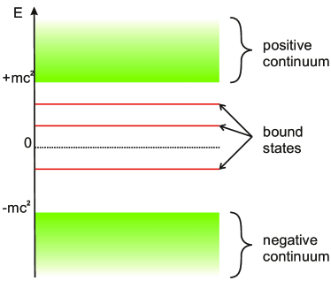
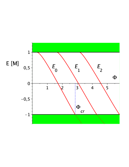
Figure 1: Typical spectrum of a Dirac Hamiltonian (left) and its dependence on the strength of an attractive potential $\Phi$ (right). At the critical value $\Phi=\Phi_{\rm{cr}}$ the lowest bound-state $E_{0}$ (red solid line) turns to a resonance in the negative continuum (red dotted line). Next bound states $E_{1},E_{2},...$ follow for larger values of $\Phi$.

The bound-state energies $E_{n}$ depend continuously on the parameters of the potential. In particular, as the strength of the negative potential $|\Phi|$ increases each $E_{n}\searrow-M$. Already at a finite value $\Phi_{\rm{cr}}$, called critical, the lowest lying bound state $E_{0}$ reaches the negative continuous spectrum associated with the interpretation of antiparticles, i.e. $E_{0}|_{\Phi=\Phi_{\rm{cr}}}=-M$. For supercritical strength of the potential $|\Phi|>|\Phi_{\rm{cr}}|$ the bound state – corresponding to a real pole in the resolvent of $\mathcal{H}$ (or in the scattering operator) – turns to a resonance (complex pole) with $\mbox{Re}(E_{0})<-M$ (see Fig. 1).

Imagine now a time-dependent process in which $\Phi(t)$ is slowly varied between the sub- and supercritical regimes as in Fig. 2.

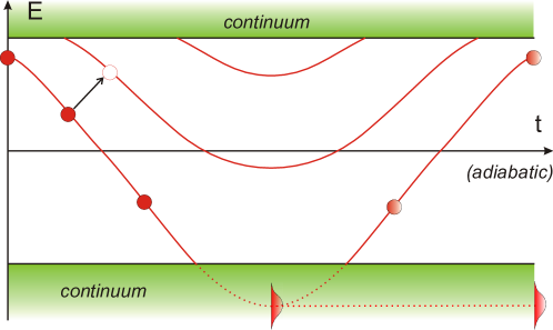
Figure 2: Spectrum of the Dirac Hamiltonian ${\cal H}(t)$ in presence of a slowly varying potential $\Phi(t)$. In the middle, a supercritical phase: the lowest bound-state (red solid line) enters the negative continuum and turns to a resonance (red dotted line).

In agreement with the adiabatic theorem, in the subcritical phase, the quantum state of the system follows the eigenstate in which it is initially prepared. As the supercritical phase begins the gap closes and the adiabatic theorem breaks down [26, 27]. The system follows then a resonance which is spectrally represented by a wave packet with position and width varying in time. Such wave packets inevitably decay in the lower continuum, trapping a big part of the wave function. Therefore, during the switch-off phase, when the potential $\Phi(t)$ becomes subcritical again, only a small part of the wave function follows the re-appearing eigenstate. Mathematically, there exists a non-vanishing matrix element of the scattering operator between the positive ($+$) and negative ($-$) continuum, $S^{+-}\neq 0$, which tends to one in the “adiabatic limit”. In order to avoid interpretational problems we need to leave the one-particle picture at this stage and switch to the many-particle description. In the language of second quantization, the discussed process is described by the scattering operator $\hat{S}$ acting in a Fock space and it can be determined from the one-particle counterpart [28]. It involves dynamical and spontaneous creation of pairs as well as annihilation and scattering of already present particles and antiparticles. In the “adiabatic limit”, the dynamical pair production goes to zero such that only the spontaneous process remains. Therefore, for processes (as described above) starting from a vacuum state $|\Omega\rangle$ and running through a supercritical phase we obtain [26, 29]

$$|\Omega\rangle\quad\longrightarrow\quad\hat{S}|\Omega\rangle=\hat{a}{}^{\dagger}\hat{b}{}^{\dagger}|\Omega\rangle$$ (4)

while for subcritical processes $|\Omega\rangle\rightarrow|\Omega\rangle$, in agreement with the adiabatic theorem. This phenomenon is called spontaneous pair creation, as opposed to the dynamical pair creation, since it is related to the spontaneous decay of a time-dependent ground state $|\Omega(t)\rangle$ (in the so called Furry picture) during the supercritical phase [30, 29].

3 Discretized quantum Dirac field

In this section we make the first step towards the quantum simulator of a quantum Dirac field in optical lattices and discretize the theory by introducing a regular lattice in space. We will argue that the phenomena of strong external fields like the supercriticality and spontaneous pair creation discussed above will survive this operation.

The Hamiltonian for the classical Dirac field reads

$$H=\int dx\,{\Psi}{}^{\dagger}(-i\sigma_{2}\partial_{x}+M\sigma_{3}+\Phi)\Psi\,.$$ (5)

We introduce a regular grid (lattice) $x_{n}=n\cdot\ell$ with a positive grid (lattice) constant $\ell$ and integers $n\in\mathbb{Z}$. The discretization of the wave function $\Psi_{n}(t):=\sqrt{\ell}\,\Psi(t,x_{n})$, defined now at the grid points $x_{n}$, gives rise to a discretized derivative $\sqrt{\ell}\,\partial_{x}\Psi(t,x_{n})\to[\Psi_{n+1}(t)-\Psi_{n-1}(t)]/(2\ell)$ and to a discretized potential $\Phi_{n}:=\Phi(x_{n})$. Finally, replacing the $x$-integral by a sum, we obtain

$$H_{d}=\sum_{n}\Psi{}^{\dagger}_{n}\left[-\frac{i\sigma_{2}}{2\ell}(\Psi_{n+1}-\Psi_{n-1})+M\sigma_{3}\Psi_{n}+\Phi_{n}\Psi_{n}\right].$$ (6)

In order to obtain the quantum many-body Hamiltonian, we quantize the discretized Dirac field operators via the fermionic anti-commutation relations

$$\{\hat{\Psi}_{n}^{\alpha}(t),[\hat{\Psi}_{m}^{\beta}(t)]{}^{\dagger}\}=\delta_{nm}\delta^{\alpha\beta}\,,\qquad\{\hat{\Psi}_{n}^{\alpha}(t),\hat{\Psi}_{m}^{\beta}(t)\}=0\;.$$ (7)

Substituting $\hat{\Psi}_{n}^{1}=\hat{a}_{n}$ and $\hat{\Psi}_{n}^{2}=\hat{b}_{n}$ the discretized many-particle Hamiltonian obtains the form

$$\hat{H} = \frac{1}{2\ell}\sum_{n}\left[\hat{b}^{\dagger}_{n+1}\hat{a}_{n}-\hat{b}^{\dagger}_{n}\hat{a}_{n+1}+{\rm{h.c.}}\right]+\sum_{n}\left[(\Phi_{n}+M)\hat{a}{}^{\dagger}_{n}\hat{a}_{n}+(\Phi_{n}-M)\hat{b}{}^{\dagger}_{n}\hat{b}_{n}\right]\,.$$ (8)

The first term describes jumping between the neighboring grid points while the remaining two terms can be treated as a combination of external potentials. Due to the specific form of the jumping, the lattice splits into two disconnected sub-lattices: (A) containing $\hat{a}_{2n}$ and $\hat{b}_{2n+1}$ and (B) containing $\hat{a}_{2n+1}$ and $\hat{b}_{2n}$ with integers $n$. Since the two sub-lattices behave basically in the same way, it is sufficient to consider only one of them, say A. With a re-definition of the local phases via $\hat{a}_{2n}\to(-1)^{n}\hat{a}_{2n}$ and $\hat{b}_{2n+1}\to(-1)^{n+1}\hat{b}_{2n+1}$, we obtain (for sub-lattice A)

$$\hat{H} = -\frac{1}{2\ell}\sum_{n}\left[\hat{b}{}^{\dagger}_{2n+1}\hat{a}_{2n}+\hat{b}{}^{\dagger}_{2n-1}\hat{a}_{2n}+{\rm{h.c.}}\right]+$$

$$+\sum_{n}\left[(\Phi_{n}+M)\hat{a}{}^{\dagger}_{2n}\hat{a}_{2n}+(\Phi_{n}-M)\hat{b}{}^{\dagger}_{2n+1}\hat{b}_{2n+1}\right]\,.$$

Identifying $\hat{c}_{2n}=\hat{a}_{2n}$ and $\hat{c}_{2n+1}=\hat{b}_{2n+1}$, this takes the form of the well known Fermi-Hubbard Hamiltonian for a one-dimensional lattice

$$\hat{H}=-\frac{J}{2}\sum_{n}\left[\hat{c}{}^{\dagger}_{n+1}\hat{c}_{n}+\hat{c}{}^{\dagger}_{n}\hat{c}_{n+1}\right]+\sum_{n}V_{n}\hat{c}{}^{\dagger}_{n}\hat{c}_{n}\,,$$ (10)

with hopping rate $J=1/\ell$ and on-site potentials $V_{n}=\Phi_{n}+(-1)^{n}M$. This Hamiltonian will be the starting point for the design of the optical lattice analogy.

Alternatively, using a more abstract language of modern quantum field theory, the Hamiltonian $\hat{H}$, being an operator acting on the Fock space ${\cal F}$, can be directly obtained by implementation of the discretized single-particle Hamiltonian

$$\mathcal{H}_{d}\Psi_{n}=-\frac{i}{2\ell}\sigma_{2}(\Psi_{n+1}-\Psi_{n-1})+M\sigma_{3}\Psi_{n}+\Phi_{n}\Psi_{n}$$ (11)

acting in the discretized Hilbert space $\mathfrak{H}_{d}=(L^{2}(\mathbb{Z}))^{2}$ (which is the discretization of $\mathfrak{H}=L^{2}(\mathbb{R})^{2}$) as a self-adjoint operator in the Fock space ${\cal F}$ according to

$$\eqalign{\hat{H}&=\sum_{n}\hat{\Psi}^{*}(\mathcal{H}f_{n})\hat{\Psi}(f_{n})=\frac{1}{2\ell}\sum_{n}\left[\hat{\Psi}^{2\,\dagger}_{n+1}\hat{\Psi}^{1}_{n}-\hat{\Psi}^{2}_{n}{}^{\dagger}\hat{\Psi}^{1}_{n+1}+{\rm{h.c.}}\right]\\ &+\sum_{n}\left[(\Phi_{n}+M)\hat{\Psi}_{n}^{1}{}^{\dagger}\hat{\Psi}_{n}^{1}+(\Phi_{n}-M)\hat{\Psi}_{n}^{2}{}^{\dagger}\hat{\Psi}_{n}^{2}\right].}$$ (14)

where the second quantized discretized Dirac field operator

$$\hat{\Psi}^{\alpha}_{n}:=\hat{\Psi}^{\alpha}(f_{n})=\int dx\,\hat{\Psi}^{\alpha}(x)f_{n}^{*}(x)$$ (15)

satisfies the above anti-commutation relations and the orthonormal set of basis functions $f_{n}$ spans the discretized Hilbert space $\mathfrak{H}_{d}$. (Here, no charge conjugation or renormalization is needed as we will physically deal with finite systems only.)

3.1 Spectrum

The free part $\hat{H}_{0}$ of this Hamiltonian, i.e., without the external potential $\Phi_{n}=0$, can be explicitly diagonalized. Performing a discrete Fourier transform on the lattice

$$\hat{a}(p):=\sum_{n}e^{-i2n\ell p}\hat{a}_{2n},\quad\hat{b}(p):=\sum_{n}e^{-i(2n+1)\ell p}\hat{b}_{2n+1},$$ (16)

for $p\in\left[-\pi/2\ell,+\pi/2\ell\right)$, where the anti-commutation relations (7) imply

$$\{\hat{a}(p),\hat{a}(q){}^{\dagger}\}=\frac{\pi}{\ell}\delta(p-q),\qquad\{\hat{a}(p){}^{\dagger},\hat{a}(q){}^{\dagger}\}=\{\hat{a}(p),\hat{a}(q)\}=0,$$ (17)

we obtain

$$\hat{H}_{0}=\frac{\ell}{\pi}\int_{-\pi/2\ell}^{\pi/2\ell}dp\left[M\left(\hat{a}(p){}^{\dagger}\hat{a}(p)-\hat{b}(p){}^{\dagger}\hat{b}(p)\right)+\frac{1}{\ell}\cos(\ell p)\left(\hat{a}(p){}^{\dagger}\hat{b}(p)+\hat{b}(p){}^{\dagger}\hat{a}(p)\right)\right]\,.$$ (18)

This Hamiltonian can be diagonalized via a unitary transformation mixing the two types of operators

$$\left(\begin{array}[]{l}\hat{A}(p)\\ \hat{B}(p)\end{array}\right)=U(p)\left(\begin{array}[]{c}\hat{a}(p)\\ \hat{b}(p)\end{array}\right)$$ (19)

with the explicit form

$$U(p)=\frac{1}{\sqrt{2E}}\left(\begin{array}[]{cc}\sqrt{E+M}&\sqrt{E-M}\\ -\sqrt{E-M}&\sqrt{E+M}\end{array}\right)$$ (20)

what leads to

$$\hat{H}_{0}=\frac{\ell}{\pi}\int_{-\pi/2\ell}^{\pi/2\ell}dp\,E(p)\left[\hat{A}(p){}^{\dagger}\hat{A}(p)-\hat{B}(p){}^{\dagger}\hat{B}(p)\right]$$ (21)

with the energy-momentum relation

$$E(p)=\sqrt{M^{2}+\frac{1}{\ell^{2}}\cos^{2}(\ell p)}\,.$$ (22)

Due to two effective types of fermionic excitations, $\hat{A}(p)$ and $\hat{B}(p)$, which enter the Hamiltonian with opposite energy signs, we obtain two symmetric energy bands separated by a gap of $2M$. Each approximates the relativistic energy-momentum relation at the edge of the Brillouin zone, for $p\approx\pm\pi/(2\ell)$. In order to obtain a positive Hamiltonian, we can perform the usual re-definition $\hat{B}(p)^{\dagger}\leftrightarrow\hat{B}(p)$ which corresponds to changing the vacuum state by filling all $\hat{B}(p)$ states with fermions. This is analogous to the Dirac sea picture in full quantum electrodynamics. In terms of this analogy, $\hat{A}(p)^{\dagger}$ or $\hat{A}(p)$ create or annihilate an electron whereas $\hat{B}(p)$ or $\hat{B}(p)^{\dagger}$ create or annihilate a positron. An additional potential $\Phi_{n}$, if sufficiently localized in space, will not modify this spectrum but may introduce bound states (isolated eigenvalues) with energies lying in the gap [31].

3.2 Supercritical potential

As an example for demonstration of supercriticality in the discretized system we consider the attractive Woods-Saxon potential

$$\Phi(x)=-\frac{W}{1+e^{a(|x|-L)}},\qquad W,a,L>0,$$ (23)

for which the one-dimensional Dirac equation is analytically solvable in terms of hypergeometric functions. The bound-state energies $E_{n}$ are determined by the equation

$$\frac{B(-2g,g+s-\lambda)^{2}}{B(2g,-g+s+\lambda)^{2}}=e^{4gaL}\frac{(s-g)^{2}-\lambda^{2}}{(s+g)^{2}-\lambda^{2}},\qquad B(x,y):=\frac{\Gamma(x)\Gamma(y)}{\Gamma(x+y)}$$ (24)

with $s:=\sqrt{M^{2}-E^{2}}/a,g:=i\sqrt{(E+W)^{2}-M^{2}}/a,\lambda:=iW/a$ and depend continuously on the parameters of the potential [32].

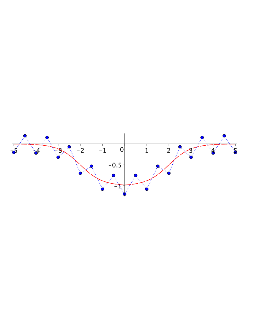
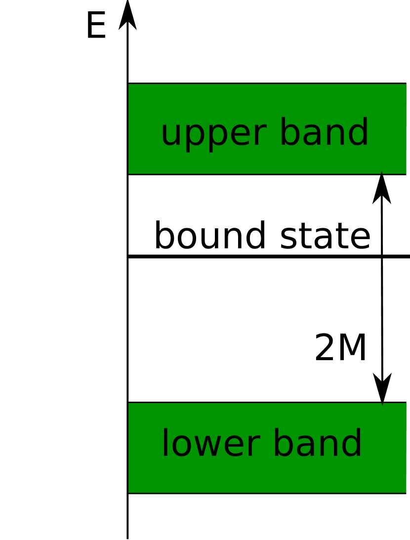
Figure 3: Left: The continuous Woods-Saxon potential $\Phi(x)$ (red dashed line) and the discretized effective potential $\Phi_{n}+(-1)^{n}M$ (blue dots, connected with dotted line for visualization only). Right: The corresponding energy spectrum. (Not to scale.)

Below, we compare the spectra of the continuous and the discretized Dirac equations with the Woods-Saxon potential. In the latter case, the discretized Woods-Saxon potential is defined by $\Phi_{n}:=\Phi(x_{n})$ with $x_{n}=\ell\cdot n$ (see Fig. 3). For both cases we calculate numerically the lowest-lying bound state $E_{0}$ as a function of the parameter $W$ ($a$ and $L$ fixed) which is a monotone function with $dE_{0}/dW<0$ as long as $-M<E_{0}<M$. The dependence of the bound state energies $\tilde{E}_{0}(W)$ for the Hubbard Hamiltonian (10) on the parameter $W$ is qualitatively the same and quantitatively in very good agreement with the curve $E_{0}(W)$ obtained as solution of (24) in the continuous case. At almost the same critical value $W_{\rm{cr}}\approx 2.878$ both bound states disappear from the spectrum and turn into complex resonances. The curves are compared in Fig. 4.

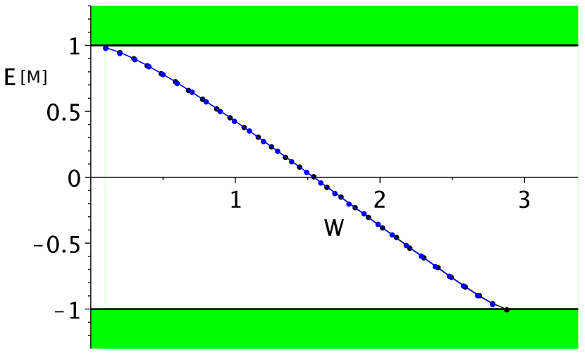
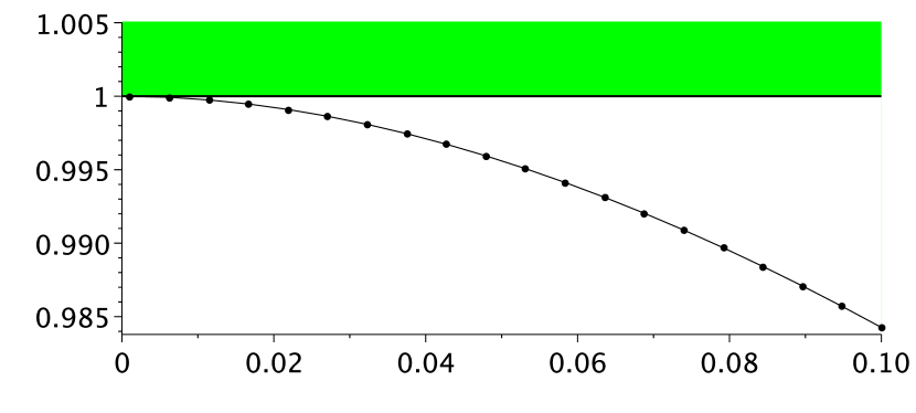
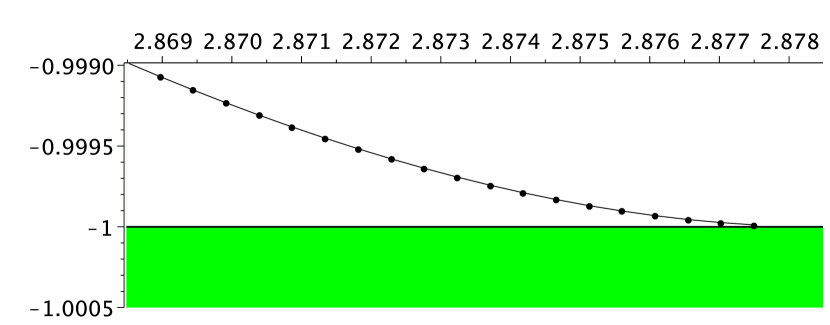
Figure 4: Comparison of the bound state energy $E$ as a function of the potential strength $W$ for the continuous (black dots and line) and discretized (blue dots and line) Dirac equation with Woods-Saxon potential (23) ($a=10,L=1$). On the right, the parabolic approach, $E(W)\approx\pm M+C_{\pm}(W-W_{\pm})^{2}$, to the upper and lower continuum.

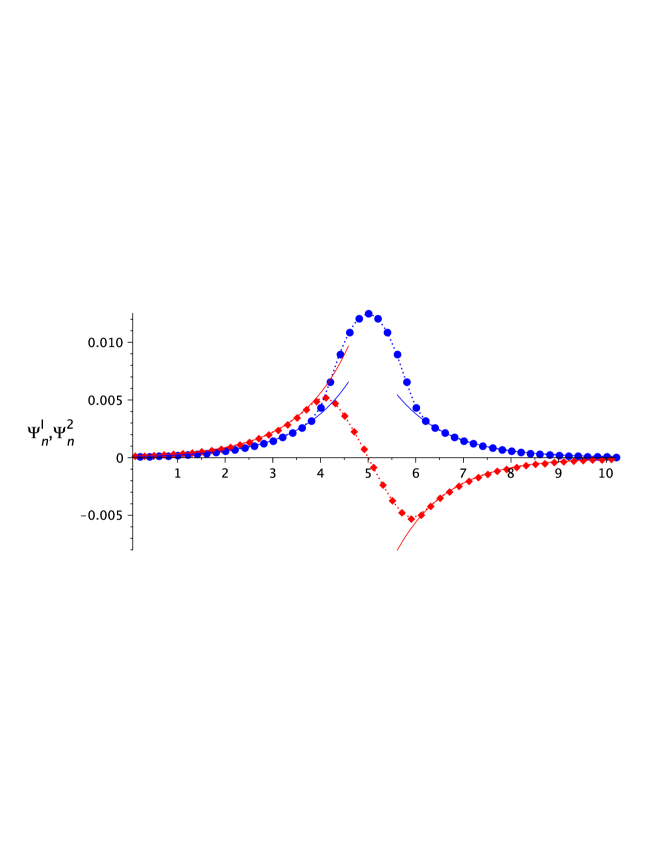
Figure 5: Typical profile of a bound state (here $E=-0.37M$). Plotted are two components of the wave function $\Psi^{1}_{n},\Psi^{2}_{n}$ (blue dots and red diamonds) against $x=n\cdot d$, supplemented by exponential asymptotes (blue and red solid lines). One function has always one zero and the other has no zeros like in the continuous Dirac equation.

4 Quantum simulator

4.1 Ultra-cold atoms in optical lattices

The main goal of this work is to propose a physical quantum system, composed of ultra-cold atoms moving in a specially designed periodic potential, which can effectively be described with a Fermi-Hubbard-type Hamiltonian of the form (10) and pseudo-relativistic dispersion relation (22) approximating the relativistic formula $E^{2}=M^{2}+p^{2}$ for energies around the Fermi-level. Moreover, excitations of the ground state should behave like particles and antiparticles and obey the Fermi statistics.

Ultra-cold atoms loaded into optical lattices are conveniently described by effective discrete Hubbard-type Hamiltonians [34]. That kind of approximation is based on a construction of a set of orthonormal wave functions $\psi_{n}$ (Wannier functions) localized around the local minima of the potential $W(x)$, giving rise to a regular grid of sites, and on the assumption that the single-particle Hamiltonian ${\cal H}$ is approximately tri-diagonal in that basis, i.e. $\left<\psi_{n}|{\cal H}|\psi_{m}\right>\approx 0$ for $|n-m|>1$. In consequence, the many-body Hamiltonian can be written in the form (10) with $J_{n}=\left<\psi_{n}|{\cal H}|\psi_{n+1}\right>$ and $V_{n}=\left<\psi_{n}|{\cal H}|\psi_{n}\right>$. There is a deeper connection between that approximation, in which only the lowest energy band is taken into account in the construction of the Wannier functions, and a spatial discretization of the theory in which the discretization step (equal to the period of the potential) introduces a natural cut-off in energies. In the latter approximation, the coefficients $J_{n}$ and $V_{n}$ correspond to the discretized kinetic (Laplacian) and potential terms in the Hamiltonian. In both approaches the energy spectrum is reduced to a single band.

4.2 Bi-chromatic optical lattice

It turns out that the emergence of a pseudo-relativistic dispersion relation, as in Eq. (22), is a quite universal phenomenon, see also [35, 36]. Imagine, we start with a periodic potential in one spatial dimension and introduce a small perturbation which breaks the original periodicity and is only periodic with the double period. This implies that the Brillouin zone $[-\pi/(2\ell),\pi/(2\ell)]$ shrinks by a factor of two and that the lowest band splits into two sub-bands. Since, at the same time, the perturbation is small the energy-momentum relation $E(p)$ at any given momentum $p$ can only change by a small amount. In consequence, the perturbation will induce significant changes only in the vicinity of the momenta $p_{0}=\pm\pi/(2\ell)$, i.e. edges of the shrinked Brillouin zone, at which it generates a small gap in the spectrum which separates the two branches of $E(p)$, see Figure 6. For small perturbations, this gap will be proportional to the amplitude of the perturbation [35, 36]. Altogether, we reproduce the pseudo-relativistic dispersion relation in the vicinity of those points $p_{0}$.

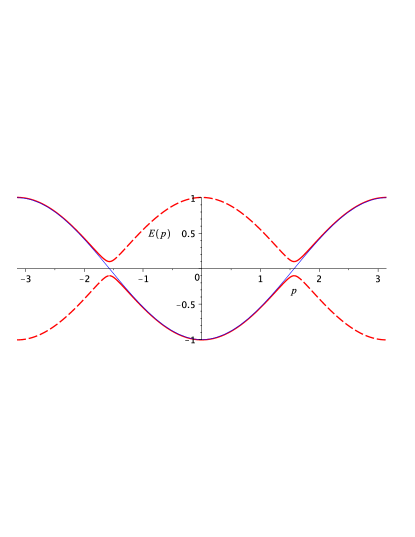
Figure 6: Sketch of the typical dispersion relation for a periodic potential (solid blue line) and perturbed doubly-periodic one (dashed red curves).

The conditions for a quantum simulator formulated above can be satisfied, in a good approximation, with ultra-cold fermionic atoms loaded into a one-dimensional optical lattice with the doubly-periodic potential

$$W(x)=W_{0}\sin^{2}(2kx)+\Delta W\sin^{2}(kx)\,,$$ (25)

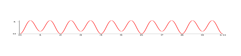
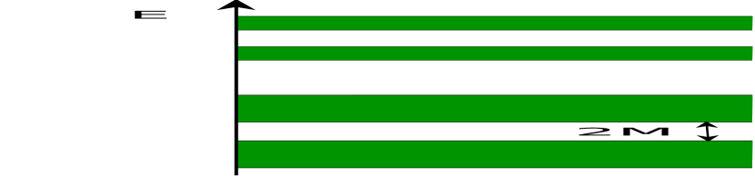
Figure 7: Left: Doubly-periodic potential $W(x)$. Right: The corresponding energy spectrum with the gap $2M\approx\Delta W$ between the lowest two bands. (Not to scale.)

where $k=\pi/(2\ell)$, by taking $W_{0}\gg\Delta W$ (see Fig. 7). Potentials of that form can be obtained by superposition of two lattice-generating standing laser waves with different frequencies. Similar settings have already been obtained experimentally [37].

Unfortunately, it is not possible to find a closed analytic formula for the energy-momentum dependence in that potential. However, by applying a version of the WKB method for periodic potentials [38] to the doubly-periodic case we were able to derive [36] a spectral condition from which an approximate dispersion relation can be calculated analytically. That condition reads

$$\cos^{2}(\Phi/2)=(1-T)\,\sin^{2}(\Delta\Phi)+T\,\cos^{2}(\ell p).$$ (26)

where $T(E)$ is the WKB-transmission coefficient through a single potential barrier [around a maximum of $W(x)$], $\Phi:=\Phi_{1}+\Phi_{2}$ and $\Delta\Phi=\Phi_{1}-\Phi_{2}$ with the WKB phases

$$\Phi_{i}(E):=\int_{y_{i}}^{z_{i}}\sqrt{E-W(x)}\,dx$$ (27)

calculated between two consecutive turning points $y_{i},z_{i}$ corresponding to the same potential minimum for which $W(y_{i})=W(z_{i})=E$ and $W(x)<E$ for $y_{i}<x<z_{i}$. The index $i=1,2$ refers to two different types of the potential minima (lower and upper).

For large $W_{0}\gg\Delta W$, the lowest energy band is narrow and lies well below the potential maximum $W_{0}$. It implies small tunneling probability $T(E)$ and small $\Delta\Phi(E)$ which are both relatively insensitive to $E$. The average phase can be approximated by a linear function $\Phi(E)\approx\alpha(E-E_{0})$ around the value $\pi$ [first minimum of $\cos^{2}(\Phi/2)$] which leads to the effective universal relation

$$E(p)-E_{0}\approx\pm\sqrt{M^{2}+J^{2}\cos^{2}(\ell p)}$$ (28)

where $M:=(1-T)\,\sin^{2}(\Delta\Phi)/\alpha^{2}$ and $J^{2}:=T/\alpha^{2}$. The approximation holds uniformly for all $p\in(-\pi/2\ell,\pi/2\ell)$ as long as $\Delta W\ll W_{0}$ (for more details, see [36]). Using again the WKB approximation, we can estimate the parameters

$$J\approx\frac{4}{\pi}\,\sqrt{W_{0}E_{R}}\,\exp\left\{-\frac{\pi}{4}\sqrt{\frac{W_{0}}{E_{R}}}\right\},\qquad M\approx\frac{\Delta W}{2}$$ (29)

where $E_{R}=k^{2}/(2M_{\rm{atom}})=\pi^{2}/(8M_{\rm{atom}}a^{2})$ is the recoil energy and $M_{\rm{atom}}$ the mass of the atoms moving in the doubly-periodic potential $W(x)$.

4.3 Wannier functions and sites

Let us discuss the transition from the simply periodic potential to the doubly periodic one on the level of the associated Hamiltonian. Starting with the single-particle Schrödinger Hamiltonian describing atoms in an external potential

$$\hat{H}=-\frac{1}{2M_{{\rm{atom}}}}\nabla^{2}+W(x)$$ (30)

and performing the standard steps we obtain, for the original periodic potential $W(x)=W_{0}\sin^{2}(2kx)$, the usual second-quantized Hamiltonian in momentum space

$$\hat{H}_{\rm original}=\frac{\ell}{2\pi}\int_{-\pi/\ell}^{\pi/\ell}dp\,E_{\rm original}(p)\,\hat{\psi}{}^{\dagger}(p)\hat{\psi}(p)\,,$$ (31)

where we consider the lowest band only with $E_{\rm original}(p)\approx-J\cos(\ell p)$ (for convenience we shifted the energy scale by the constant $E_{0}$ what has no physical consequences). After switching on the doubly-periodic perturbation $\Delta W\sin^{2}(kx)$, the energy spectrum undergoes a transition $E_{\rm original}(p)\rightarrow E(p)\approx\pm\sqrt{M^{2}+J^{2}\cos^{2}(\ell p)}$ and the Hamiltonian becomes

$$\hat{H}=\frac{\ell}{\pi}\int_{-\pi/2\ell}^{\pi/2\ell}dp\,\left(\begin{array}[]{c}\hat{\chi}(p)\\ \hat{\psi}(p)\end{array}\right)^{\dagger}{\cal M}\left(\begin{array}[]{c}\hat{\chi}(p)\\ \hat{\psi}(p)\end{array}\right)$$ (32)

with $\hat{\chi}(p):=\hat{\psi}(p+\pi)$ [assuming periodicity $\hat{\psi}(p+2\pi)=\hat{\psi}(p)$] and

$${\cal M}=\left(\begin{array}[]{cc}\sqrt{M^{2}+J^{2}\cos^{2}(\ell p)}&0\\ 0&-\sqrt{M^{2}+J^{2}\cos^{2}(\ell p)}\end{array}\right).$$ (33)

This Hamiltonian has the same form as the one for the discretized Dirac equation (21) when we set $J=1/\ell$.

For the two separated energy bands there exist two separate sets of Wannier functions on the lattice: the “lower” and the “upper” centered at even and odd sites, respectively. But these Wannier functions turn out to be poorly localized on the lattice (somewhat analogously to continuous quantum field theory where free particles with fixed energy are not localized in space). In order to achieve optimal localization it is preferred to switch to the set of operators introduced already in (19)-(20)

$$\left(\begin{array}[]{c}\hat{a}(p)\\ \hat{b}(p)\end{array}\right)=U(p){}^{\dagger}\left(\begin{array}[]{c}\hat{\chi}(p)\\ \hat{\psi}(p)\end{array}\right)$$ (34)

what transforms the matrix ${\cal M}$ via the similarity transformation ${\cal M}^{\prime}=U{}^{\dagger}{\cal M}U$ to

$${\cal M}^{\prime}=\left(\begin{array}[]{cc}M&J\cos(\ell p)\\ J\cos(\ell p)&-M\end{array}\right).$$ (35)

Now, going from the momentum to the site representation by inverting the Fourier transformation (16)

$$\hat{a}_{2n}=\frac{\ell}{\pi}\int_{-\pi/2\ell}^{\pi/2\ell}dp\,e^{2in\ell p}\hat{a}(p)\,,\qquad\hat{b}_{2n+1}=\frac{\ell}{\pi}\int_{-\pi/2\ell}^{\pi/2\ell}dp\,e^{i(2n+1)\ell p}\hat{b}(p)\,,$$ (36)

we obtain the free Hubbard Hamiltonian (3) with $J=1/(2\ell)$. By this construction $\hat{a}{}^{\dagger}_{2n}$ and $\hat{b}{}^{\dagger}_{2n+1}$ create two types of particles in two types of Wannier states exponentially localized at even and odd sites, respectively. However, they do not give rise to “positive” and “negative energy sites” as they mix energies from both bands. This can be best seen in the limiting case $M\ll J$ where the Wannier functions [up to terms ${\mathcal{O}}\left(M/J\right)$]

$$a_{2n}\cong\frac{1}{\sqrt{2}}(\chi_{2n}-\psi_{2n}),\qquad b_{2n+1}\cong\frac{1}{\sqrt{2}}(\chi_{2n+1}+\psi_{2n+1})$$ (37)

are build from the difference and sum of the single-band Wannier functions for the lower and upper bands defined as

$$\psi_{n}:=\frac{\ell}{\pi}\int_{-\pi/2\ell}^{\pi/2\ell}dp\,e^{in\ell p}\psi(p)\,,\qquad\chi_{n}:=\frac{\ell}{\pi}\int_{-\pi/2\ell}^{\pi/2\ell}dp\,e^{in\ell p}\chi(p)\,.$$ (38)

4.4 Physical parameters

In order to discuss the experimental realizability of our quantum simulator, let us summarize the conditions on the involved parameters. Strictly speaking, the WKB approximation used above requires $W_{0}\gg E_{R}$ which then implies $E_{R}\gg J$ via Eq. (29). However, even if we relax these conditions to

$$W_{0}>E_{R}>J\,,$$ (39)

we still get qualitatively the same picture. What is crucial, however, is the applicability of the single-band Fermi-Hubbard Hamiltonian  (10). To ensure this, we demand that the local oscillator frequency $\omega_{{\rm{o}}sc}$ in the potential minima be much smaller than $J$. In addition, the continuum limit – i.e., that the discretized expression (6) provides a good approximation – requires $J\gg M$, i.e., $1/\ell\gg M$. For the same reason, the change $\Delta\Phi_{n}=\Phi_{n+1}-\Phi_{n}$ of the analogue of the electrostatic potential $\Phi_{n}$ from one site to the next should be smaller than $M$. Over many sites, however, this change can well exceed the mass gap $2M$, which is basically one of the conditions for the Sauter-Schwinger effect to occur. Finally, the effective temperature $T$ should be well below the mass gap $2M$ in order to avoid thermal excitations. In summary, the analogue of the $e^{+}e^{-}$ pair creation can be simulated if the involved scales obey the hierarchy

$$\omega_{{\rm{o}}sc}\gg J\gg M\gg T\,.$$ (40)

Let us insert some example parameters. The recoil energy $E_{R}$ of ⁶Li atoms in an optical lattice made of light with a wavelength of 500 nm is around $E_{R}\approx 7\,\mu{\rm{K}}$. Thus, if we adjust the potential strength to be $W_{0}=10\,\mu{\rm{K}}$, the hopping rate $J$ would be around $5\,\mu{\rm{K}}$ which is still sufficiently below the local oscillator frequency $\omega_{{\rm{o}}sc}$ of around $34\,\mu{\rm{K}}$. Then a perturbation of $\Delta W=1\,\mu{\rm{K}}$ created by light with a wavelength of 1000 nm would induce an effective mass $M$ of 500 nK and thus the effective temperature should be below that value – which is not beyond present experimental capabilities.

5 Spontaneous pair creation on the lattice

The above established analogy between the (discretized) second quantized Dirac field describing electrons and positrons in an electric field, on the one hand, and the (Fermi or Bose, see Sec. 5.2) Hubbard model describing ultra-cold atoms in an optical lattice, on the other hand, enables laboratory simulations of some of the relativistic phenomena of strong-field QED. The original Sauter-Schwinger effect [6] with a constant electric field $E$ would correspond to a static tilted optical lattice with $\Phi(x)=Ex$ (the so called Wannier-Stark ladder, see e.g. [39]). For nonzero values of $E>0$ one would expect a constant rate of spontaneously generated particles and holes (cf. formula (1)), depending non-perturbatively on $E$. However, a constant electric field $E$ is unrealistic from an experimental point of view. An electric field which is localized in space and time is simpler to handle both, experimentally and conceptually (see e.g. [7, 40]). Therefore, in the following we discuss the process of analogue spontaneous pair creation in presence of an external localized potential which will be slowly switched on to a supercritical value – admitting one bound state to dive into the negative continuum – and then switched off, as discussed in Sec 2. In presence of the attractive potential a bound state will form in the gap $2M$ between the two lowest bands (formed from the lowest band splitted due to the doubly-periodic perturbation). During the time-dependent process, the bound state will slowly reach the lower band and then turn into a resonance lying within this band (see Fig. 8). The resonance will then decay causing an instability of the Fermi state (our analogue vacuum state) which will spontaneously decay to an energetically more favorable state with a particle-hole pair present. The “particle” (an atom excited above the Fermi level) will stay bound by the attractive potential while the “antiparticle” (hole in the Fermi sea) will be in a scattering state.

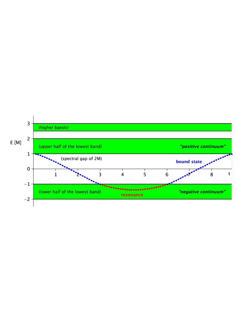
Figure 8: Time-dependent bound state/resonance interpolating between two halves of the lowest energy band after splitting it by a doubly-periodic perturbation of the optical potential. (Bands and gap not to scale.)

5.1 Experimental procedure

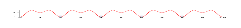
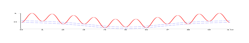
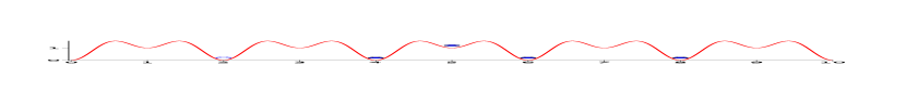
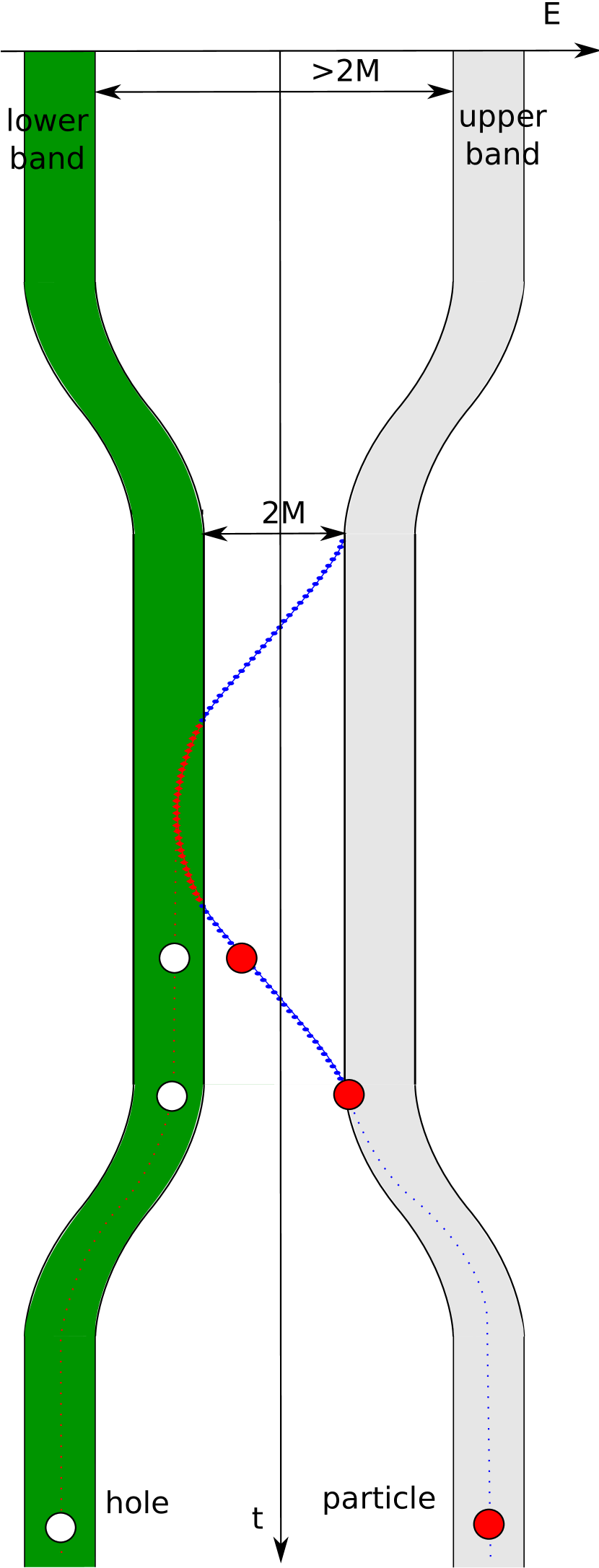
Figure 9: Sketch (not to scale) of the stages of the simulation (from top to bottom). Left: The solid red curves represent the sum of the optical lattice potential $W(x)$ and the dynamically switched supercritical potential $\Phi(x)$ as a function of position $x$ while the dashed blue curves correspond to the effective electric potential $\Phi$. The blue solid dots are particles and the empty circle is a hole. Right: Band structure and a bound state changing in time.

Simulation of the “pair production” in the optical lattice requires preparation of the initial quantum state of the atoms corresponding to the Dirac sea in QED. This can be achieved by keeping a large value of $\Delta W$ (separation of two bands by a large gap) during the cooling phase and generating a clear Fermi level at half filling of the lattice (all particles in the lower sites, see Fig. 9, top). Next, the value of $\Delta W$ should be adiabatically decreased to values well below $W_{0}$ to achieve $M\ll J$ and allow the atoms for dispersion across the lattice. The atoms become delocalized but still the lower band is fully filled while the upper band remains empty (second picture in Fig. 9). Then the “external” potential $\Phi$ (which mimics the electric potential) can be slowly switched on to reach a supercritical value. In that phase, the ground state (“vacuum”) will get rearranged via tunneling from the lower band to the upper band (analogue of the Sauter-Schwinger effect, third picture in Fig. 9). Such an created particle-hole pair will tend to separate on the lattice so that when the potential is slowly switched off after some delay the pair will not be able to annihilate any more (fourth picture in Fig. 9). That mimics the well known spontaneous pair creation known from QED. Finally, in order to detect the “pair” in experiment, the value of $\Delta W$ can be adiabatically increased again thus leading to energetic separation of the created particle and hole represented by an atom in one of the upper minima and a missing atom in one of the lower minima (fifth picture in Fig. 9). The atom in one of the upper sites and the hole (missing atom) in one of the lower minima could be detected via site-resolved imaging [41]. Another option could be blue-sideband-detuned optical transitions which are resonant to the oscillation frequency $\omega_{osc}$ of the upper minima but not to those in the lower sites.

5.2 Bose-Fermi mapping

Since it is typically easier to cool down bosonic than fermionic atoms, let us discuss an alternative realization based on bosons in an optical lattice. To this end, we start with the Bose-Hubbard Hamiltonian

$$\hat{H}=-J\sum_{n}\left[\hat{d}{}^{\dagger}_{n+1}\hat{d}_{n}+\hat{d}{}^{\dagger}_{n}\hat{d}_{n+1}\right]+\sum_{n}V_{n}\hat{d}{}^{\dagger}_{n}\hat{d}_{n}+\frac{U}{2}\sum_{n}(\hat{d}^{\dagger}_{n})^{2}\,\hat{d}_{n}^{2}\,,$$ (41)

which has the same form as the Fermi-Hubbard Hamiltonian (3) after replacing the fermionic $\hat{c}_{n}$ by bosonic $\hat{d}_{n}$ operators, but with an additional on-site repulsion term $U$. For large $U\gg J$ (which can be controlled by an external magnetic field via a Feshbach resonance, for example), we obtain the bosonic analogue of “Pauli blocking”, i.e., at most one particle can occupy each site $\hat{d}_{n}^{2}\left|\Psi\right>\approx 0$. Neglecting all states with double or higher occupancy, we can map these bosons exactly onto fermions in one spatial dimension via

$$\hat{d}_{n}=\exp\left(-i\pi\sum_{m<n}\hat{c}{}^{\dagger}_{m}\hat{c}_{m}\right)\hat{c}_{n}\,.$$ (42)

Via this transformation, the bosonic commutation relations $[\hat{d}_{n},\hat{d}^{\dagger}_{m}]=\delta_{nm}$ and $[\hat{d}^{\dagger}_{n},\hat{d}^{\dagger}_{m}]=[\hat{d}_{n},\hat{d}_{m}]=0$ are exactly mapped onto the fermionic anti-commutation relations $\{\hat{c}_{n},\hat{c}^{\dagger}_{m}\}=\delta_{nm}$ and $\{\hat{c}_{n},\hat{c}_{m}\}=\{\hat{c}^{\dagger}_{n},\hat{c}^{\dagger}_{m}\}=0$. As a result, we obtain the same physics as described by the Fermi-Hubbard Hamiltonian (3).

5.3 Interactions

Apart from investigating the pair creation probability for space-time dependent electric fields $E(t,x)$, this quantum simulator for the Sauter-Schwinger effect could provide some insight into the impact of interactions. For example, including dipolar interactions of the atoms, we would get the coupling Hamiltonian $D_{nm}\hat{c}{}^{\dagger}_{n}\hat{c}{}^{\dagger}_{m}\hat{c}_{n}\hat{c}_{m}$ with $D_{nm}\propto|n-m|^{-3}$. As an example for permanent dipole moments, we may consider ⁵²Cr atoms possessing a rather large magnetic moment. However, the associated interaction energy $D_{nm}$ would be below one nano-Kelvin and thus probably too small to generate significant effects. Therefore, let us consider externally induced dipole moments. For example, ⁶Li atoms can be electrically polarized by an external electric field of order $10^{8}~{}{\rm{V}}/m$ (which can be realized experimentally) such that the induced electric dipole moments generate interaction energies up to a few $\mu$K. By aligning the atomic dipole moments parallel or perpendicular to the lattice, we may even switch between attractive $D_{nm}<0$ and repulsive $D_{nm}>0$ interactions. Note that this goes far beyond the simulation of the classical Dirac equation and requires the full quantum many-particle Hamiltonian.

Appendix A Potential localized at one site (delta-like)

In order to compare the discretized Dirac Hamiltonian with its continuum version, we consider an example where both can be solved analytically. This is possible for a Dirac delta like potential localized at one lattice site

$$\phi_{n}=\phi\,\frac{\delta_{0,n}}{\ell}\qquad{\rm{with}}\qquad\phi(p)=\phi$$ (43)

which corresponds to $\phi(x)=\phi\,\delta(x)$ in the continuous case $\ell\rightarrow 0$. It has the advantage that a closed formula for the bound-state energy can be found analytically. The Hubbard Hamiltonian (18) with added potential reads then

$$\hat{H} = \frac{\ell}{\pi}\int_{-\pi/2\ell}^{\pi/2\ell}dp\,\left[M\left(\hat{a}(p){}^{\dagger}\hat{a}(p)-\hat{b}(p){}^{\dagger}\hat{b}(p)\right)+J\cos(\ell p)\left(\hat{a}(p){}^{\dagger}\hat{b}(p)+\hat{b}(p){}^{\dagger}\hat{a}(p)\right)\right]+$$ (44)

$$+\frac{\phi\,\ell^{2}}{\pi^{2}}\left[\int_{-\pi/2\ell}^{\pi/2\ell}dp_{1}\,\hat{a}^{\dagger}(p_{1})\;\int_{-\pi/2\ell}^{\pi/2\ell}dp_{2}\,\hat{a}(p_{2})+\int_{-\pi/2\ell}^{\pi/2\ell}dp_{1}\,\hat{b}^{\dagger}(p_{1})\;\int_{-\pi/2\ell}^{\pi/2\ell}dp_{2}\,\hat{b}(p_{2})\right]\,,$$

where we set $J=1/\ell$. Obviously, it satisfies $\hat{H}|0\rangle=0$ for the vacuum vector $|0\rangle$ such that $\hat{a}(p)|0\rangle=\hat{b}(p)|0\rangle=0$. However, we want to find a one-particle eigenstate $|\chi\rangle$ of the Hamiltonian $\hat{H}$ with eigenvalue $\lambda$ lying in the gap $-M<\lambda<M$ (which corresponds to a bound state for the discretized Dirac equation). Then we want to study the dependence of the eigenvalue $\lambda$ on the strength of the potential $\phi$. The general one-particle state can be written as

$$|\chi\rangle=\left[\frac{\ell}{\pi}\int_{-\pi/2\ell}^{\pi/2\ell}dp\,A(p)\hat{a}{}^{\dagger}(p)+\frac{\ell}{\pi}\int_{-\pi/2\ell}^{\pi/2\ell}dp\,B(p)\hat{b}{}^{\dagger}(p)dp\right]|0\rangle$$ (45)

with two complex functions $A(p)$ and $B(p)$. By projecting the eigenvalue equation $\hat{H}|\chi\rangle=\lambda|\chi\rangle$ on the states $\langle 0|\hat{a}(p)$ and $\langle 0|\hat{b}(p)$ we arrive at a system of equations

$$\underbrace{\left(\begin{array}[]{cc}M-\lambda,&J\cos(\ell p)\\ J\cos(\ell p),&-M-\lambda\end{array}\right)}_{=:{\cal M}}\left(\begin{array}[]{c}A(p)\\ B(p)\end{array}\right)=-\phi\,\frac{\ell}{\pi}\int_{-\pi/2\ell}^{\pi/2\ell}dp\left(\begin{array}[]{c}A(p)\\ B(p)\end{array}\right).$$ (46)

Integration of both sides over $p$ leads to the relations

$$\bar{A} :=\frac{\ell}{\pi}\int_{-\pi/2\ell}^{\pi/2\ell}A(p)dp=\frac{\frac{\ell}{\pi}\int_{-\pi/2\ell}^{\pi/2\ell}dp\,J\cos(\ell p)B(p)}{\lambda-M-\phi}\,,$$

$$\bar{B} :=\frac{\ell}{\pi}\int_{-\pi/2\ell}^{\pi/2\ell}B(p)dp=\frac{\frac{\ell}{\pi}\int_{-\pi/2\ell}^{\pi/2\ell}dp\,J\cos(\ell p)A(p)}{\lambda-M-\phi}\,.$$ (47)

Observe that the right-hand side of (46) is equal to $-\phi(\bar{A},\bar{B})^{T}$. We can invert the matrix ${\cal M}$, whose determinant $\det{\cal M}=\lambda^{2}-M^{2}-J\cos^{2}(\ell p)<0$ never vanishes, to obtain

$$\left(\begin{array}[]{c}A(p)\\ B(p)\end{array}\right)=\frac{\phi}{\lambda^{2}-M^{2}-J\cos^{2}(\ell p)}\left(\begin{array}[]{cc}\lambda+M,&J\cos(\ell p)\\ J\cos(\ell p),&\lambda-M\end{array}\right)\left(\begin{array}[]{c}\bar{A}\\ \bar{B}\end{array}\right).$$ (48)

Integrating both sides over $p$ again and using

$$\frac{\ell}{\pi}\int_{-\pi/2\ell}^{\pi/2\ell}\frac{dp}{\lambda^{2}-M^{2}-J\cos^{2}(\ell p)} =-\frac{1}{\sqrt{M^{2}-\lambda^{2}}\sqrt{M^{2}+J^{2}-\lambda^{2}}}\,,$$

$$\frac{\ell}{\pi}\int_{-\pi/2\ell}^{\pi/2\ell}\frac{J\cos(\ell p)\ dp}{\lambda^{2}-M^{2}-J\cos^{2}(\ell p)} =0\,,$$ (49)

we obtain consistency conditions

$$\left(\begin{array}[]{c}\bar{A}\\ \bar{B}\end{array}\right)=\frac{-\phi}{\sqrt{M^{2}-\lambda^{2}}\sqrt{M^{2}+J^{2}-\lambda^{2}}}\left(\begin{array}[]{c}(\lambda+M)\bar{A}\\ (\lambda-M)\bar{B}\end{array}\right)$$ (54)

which cannot be satisfied at the same time except when (at least) one of the constants $\bar{A},\bar{B}$ vanishes. Assume first, it is $\bar{B}=0$ (the case $\bar{A}=0$ will be discussed below). Then we need to solve the algebraic equation

$$-\phi\frac{\lambda+M}{\sqrt{M^{2}-\lambda^{2}}\sqrt{M^{2}+J^{2}-\lambda^{2}}}=1$$ (55)

for the function $\lambda(\phi)$. It has, in general, three solutions what can be better seen from

$$(M-\lambda)(M^{2}+J^{2}-\lambda^{2})=\phi^{2}(M+\lambda)\,.$$ (56)

For $\phi=0$, these three solutions start from the points $M,\pm\sqrt{M^{2}+J^{2}}$, i.e., the edges of the continuous spectrum. We are interested in the perturbations of the eigenvalue $\lambda=M$ for negative values of $\phi$, i.e. for a bound state separating from the bottom of the upper band. For small $\phi$, $\lambda(\phi)$ behaves like $\lambda(\phi)\cong M(1-2\phi^{2})$. For increasing values of $|\phi|$ it monotonically decreases to $-M$ but never reaches this value (more precisely, $\lambda(\phi)\cong-M+2M/\phi^{2}$ for $|\phi|\gg 1$) – see Fig. 10.

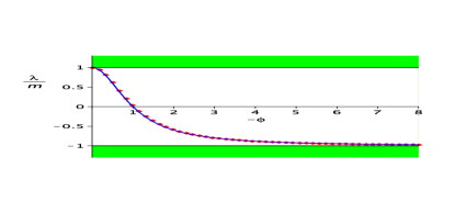
Figure 10: Left: The eigenvalue $\lambda/M$ as a function of the potential’s strength $\phi$ for the discretized Dirac equation (red solid line) compared to the continuous Dirac equation with the delta potential (blue dashed line).
Right: The momentum distribution $A(p),B(p)$ for a bound state with $\lambda=0.8M$.

It shows that there is no supercriticality in this potential, i.e., crossing of the value $\lambda(\phi)=-M$ at finite $\phi$, what is analogous to the continuous case $\phi(x)=\phi\,\delta(x)$ in which $\lambda(\phi)=M(1-\phi^{2})/(1+\phi^{2})$ [42].

From equation (48) we can also find the eigenvector to the eigenvalue $\lambda$

$$\left(\begin{array}[]{c}A(p)\\ B(p)\end{array}\right)=\frac{\phi\ \bar{A}}{\lambda^{2}-M^{2}-J\cos^{2}(\ell p)}\left(\begin{array}[]{c}\lambda+M\\ J\cos(\ell p)\end{array}\right)$$ (57)

where the value of $\bar{A}$ is to be determined from the normalization condition

$$\frac{1}{2\pi}\int_{0}^{2\pi}dp\,\left(|A(p)|^{2}+|B(p)|^{2}\right)=1\,.$$ (58)

Since both $|A(p)|^{2}$ and $|B(p)|^{2}$ are even functions of $p$, we have

$$\frac{1}{2\pi}\int_{0}^{2\pi}dp\,\left(|A(p)|^{2}+|B(p)|^{2}\right)J\cos(\ell p)=0\,,$$ (59)

which reflects the fact that the (discretized) momentum $id/dx\rightarrow J\cos(\ell p)$ vanishes in the bound state. Note also that the condition $\bar{B}=0$ implies $B_{0}=0$ what means that the “antiparticles” are repelled from the site at which the potential is localized.

The case $\bar{A}=0$ is fully analogous and the solutions can be obtained by a symmetry transformation: $\lambda\rightarrow-\lambda$ and $\phi\rightarrow-\phi$. The bound state emerges then from the lower band (negative“continuum”) at $\lambda=-M$ and goes up for positive potentials $\phi$.

Remark 1.

The considered potential is localized at one site $n=0$ in that sense that it interacts with both types of particles via $a_{0}$ and $b_{0}$. But in fact, $a_{0}$ and $b_{0}$ are two different (neighbouring) sites brought to $k=0$ by a convenient renumbering. It is also possible to consider the potential to be localized in such a way that it interacts with only one type of particles, say via $a_{0}$. Then the equations get slightly modified (the term $\bar{B}$ disappears at some places) and we obtain $\bar{B}=0$ as consequence of (48) and (A). From that point on, the solution is identically the same to the previous case. It means that it plays no role whether we consider potentials localized at one site interacting with only one or with both types of particles because, in the latter case, the solutions split into two symmetric cases of the former type.

Remark 2.

The above method of calculating $\lambda(\phi)$ works only for potentials for which $\frac{1}{2\pi}\int_{0}^{2\pi}dp\,\phi(p-q)\det{\cal M}(p)^{-1}$ is independent of $q$, i.e. for $\phi(p)=const$ which corresponds to $\phi_{n}\sim\delta_{n,0}$. Unfortunately, it cannot be generalized to more complex potentials in a simple way.

References

References

- [1]
- [2] P. A. M. Dirac Proc. Roy. Soc. (London) A 117, 610 (1928); ibid. 118, 351 (1928); ibid. 126, 360 (1930).
- [3] I. Pomeranchuk and J. Smorodinsky, J. Phys. USSR 9, 97 (1945); W. Pieper and W. Greiner, Z. Physik 218, 327–340 (1969); V. D. Mur and V. S. Popov, Theor. Math. Phys. 27, 429–438 (1976).
- [4] APEX, EPOS and ORANGE Collaborations (GSI, Frankfurt, Heidelberg, Mainz, BNL, Yale); P. Kienle, Annual Review of Nuclear and Particle Science 36, 605-648 (1986); J. S. Greenberg and W. Greiner, Physics Today, August 1982, p. 24.
- [5] See, e.g., the European ELI programme: http://www.extreme-light-infrastructure.eu/
- [6] J. Schwinger, Phys. Rev. 82, 664 (1951).
- [7] F. Sauter, Z. Phys. 69, 742 (1931); ibid. 73, 547 (1932).
- [8] W. Heisenberg and H. Euler, Z. Phys. 98, 714 (1936). V. Weisskopf, Kong. Dans. Vid. Selsk., Mat.-fys. Medd. XIV, 6 (1936).
- [9] See, e.g., A. I. Nikishov and V. I. Ritus, Sov. Phys. JETP 25, 1135 (1967); E. Brezin and C. Itzykson, Phys. Rev. D 2, 1191 (1970); F. V. Bunkin and I. I. Tugov, Sov. Phys. Dokl. 14, 678 (1970); N. B. Narozhnyi and A. I. Nikishov, Sov. J. Nucl. Phys. 11, 596 (1970); V. S. Popov, JETP Lett. 13, 185 (1971); ibid. 18, 255 (1973); S. P. Kim and D. N. Page, Phys. Rev. D 65, 105002 (2002); ibid. 75, 045013 (2007); N. B. Narozhny, S. S. Bulanov, V. D. Mur, and V. S. Popov, Phys. Lett. A 330, 1 (2004); JETP Lett. 80, 382 (2004); H. Gies and K. Klingmuller, Phys. Rev. D 72, 065001 (2005). G. V. Dunne and C. Schubert, ibid. 72, 105004 (2005); H. K. Avetissian, A. K. Avetissian, G. F. Mkrtchian, and Kh. V. Sedrakian, Phys. Rev. E 66, 016502 (2002); H. K. Avetissian, Relativistic Nonlinear Electrodynamics (Springer, New York, 2006).
- [10] R. Schützhold, H. Gies, and G. Dunne, Phys. Rev. Lett. 101, 130404 (2008); G. V. Dunne, H. Gies, and R. Schützhold, Phys. Rev. D80, 111301 (2009).
- [11] C. K. Dumlu and G. V. Dunne, Phys. Rev. Lett. 104, 250402 (2010).
- [12] Witthaut et al., ArXiv e-prints (2011), 1102.4047.
- [13] W. G. Unruh and R. Schützhold, Phys. Rev. D 68, 024008 (2003).
- [14] S. Longhi, Phys. Rev. A 81, 022118 (2010).
- [15] Dreisow et al., Phys. Rev. Lett. 105, 143902 (2010).
- [16] Gerritsma et al., Phys. Rev. Lett. 106, 060503 (2011).
- [17] Gerritsma et al., Nature 463, 68 (2010).
- [18] L. Lamata, J. León, T. Schätz, and E. Solano, Phys. Rev. Lett. 98, 253005 (2007).
- [19] S.-L. Zhu, B. Wang, and L.-M. Duan, Phys. Rev. Lett. 98, 260402 (2007).
- [20] J. I. Cirac, P. Maraner, and J. K. Pachos, Phys. Rev. Lett. 105, 190403 (2010).
- [21] J.-M. Hou, W.-X. Yang, and X.-J. Liu, Phys. Rev. A 79, 043621 (2009).
- [22] L.-K. Lim, C. M. Smith, and A. Hemmerich, Phys. Rev. Lett. 100, 130402 (2008).
- [23] Goldman et al., Phys. Rev. Lett. 103, 035301 (2009).
- [24] O. Boada, A. Celi, J. I. Latorre, and M. Lewenstein, ArXiv e-prints (2010), 1010.1716.
- [25] Novoselov et al., Nature 438, 197 (2005); M. I. Katsnelson, K. S. Novoselov, and A. K. Geim, Nature Physics 2, 620 (2006); D. Allor, T. D. Cohen and D. A. McGady, Phys. Rev. D 78, 096009 (2008); B. Dora and R. Moessner, Phys. Rev. B 81, 165431 (2010); B. Rosenstein, M. Lewkowicz, H. C. Kao and Y. Korniyenko, Phys. Rev. B 81, 041416(R) (2010); H. C. Kao, M. Lewkowicz and B. Rosenstein, Phys. Rev. B 82, 035406 (2010).
- [26] G. Nenciu. Comm. Math. Phys., 76:117–128, 1980.
- [27] G. Nenciu. Comm. Math. Phys., 109:303–312, 1987.
- [28] G. Scharf. Finite Quantum Electrodynamics - The Causal Approach, 2nd Edition. Springer Verlag Berlin Heidelberg New York, 1995.
- [29] N. Szpak, J. Phys. A: Math. Theor. 41, 164059 (2008); N. Szpak, Spontaneous particle creation in time-dependent overcritical fields of QED (PhD Thesis, University Frankfurt am Main, 2006); P. Pickl and D. Dürr, EPL 81, 40001 (2008).
- [30] J. Rafelski, B. Müller and W. Greiner, Nucl. Phys. B 68, 585–604 (1974); W. Greiner, B. Müller, and J. Rafelski, Quantum Electrodynamics of Strong Fields. Texts and Monographs in Physics. Springer-Verlag, 1985.
- [31] G. F. Koster and J. C. Slater, Phys. Rev. 95, 1167 (1954); ibid. 96, 1208 (1954); F. Bassani, G. Iadonisi and B. Preziosi, ibid. 186, 735 (1969).
- [32] P. Kennedy, J. Phys. A: Math. Gen. 35 (2002) 689-698
- [33] T. J. Maier and R. M. Dreizler, Phys. Rev. A 45, 2974 (1992).
- [34] I. Bloch, J. Dalibard and W. Zwerger, Rev. Mod. Phys. 80, 885 (2008); V.I. Yukalov, Laser Physics 19, 1–110 (2009); M. Lewenstein et al., Advances in Physics 56, 243–379 (2007); T. Esslinger, Annual Review of Condensed Matter Physics 1, 129–152 (2010).
- [35] R. Schützhold, N. Szpak, e-print arXiv:1103.0541, submitted.
- [36] N. Szpak, to appear.
- [37] T. Salger, C. Geckeler, S. Kling, and M. Weitz, Phys. Rev. Lett. 99, 190405 (2007).
- [38] N. L. Balazs, Annals of Physics 53, 421 (1969).
- [39] Q. Thommen, J. C. Garreau and V. Zehnlé, J. Opt. B: Quantum Semiclass. Opt. 6, 301–308 (2004).
- [40] P. J. M. Bongaarts and S. N. M. Ruijsenaars, Ann. Phys. 101, 289–318 (1976).
- [41] Sherson et al., Nature 467, 68 (2010).
- [42] F. Dominguez-Adame and E. Macia, J. Phys. A: Math. Gen. 22, L419 (1989); M. Loewe and M. Sanhueza, J. Phys. A: Math. Gen. 23, 553-561 (1990).