Query processing in distributed, taxonomy-based information sources

Abstract

We address the problem of answering queries over a distributed information system, storing objects indexed by terms organized in a taxonomy. The taxonomy consists of subsumption relationships between negation-free DNF formulas on terms and negation-free conjunctions of terms. In the first part of the paper, we consider the centralized case, deriving a hypergraph-based algorithm that is efficient in data complexity. In the second part of the paper, we consider the distributed case, presenting alternative ways implementing the centralized algorithm. These ways descend from two basic criteria: direct vs. query re-writing evaluation, and centralized vs. distributed data or taxonomy allocation. Combinations of these criteria allow to cover a wide spectrum of architectures, ranging from client-server to peer-to-peer. We evaluate the performance of the various architectures by simulation on a network with $O(10^{4})$ nodes, and derive final results. An extensive review of the relevant literature is finally included.

1 Introduction

Consider an information source $\mathcal{S}$ structured as a tetrad $\mathcal{S}=(T,\preceq,\mathit{Obj},I),$ where $T$ is a set of terms, $\preceq$ is a taxonomy over concepts expressed using $T$ (e.g. $\mathtt{(Animal\wedge FlyingObject})\vee\mathtt{Penguin}\preceq\mathtt{Bird}$), $\mathit{Obj}$ is a set of objects and $I$ is the interpretation, that is a function from $T$ to $\mathcal{P}(\mathit{Obj})$, assigning an extension (i.e., a set of objects) to each term. Now assume that there is a set $\mathcal{N}$ of such sources $\mathcal{N}=\{\mathcal{S}_{1},\ldots,\mathcal{S}_{n}\},$ all sharing the same set of objects $\mathit{Obj}$ and related by taxonomic relationships amongst concepts of different sources. These relationships are called articulations and aim at bridging the inevitable naming, granularity and contextual heterogeneities that may exist between the taxonomies of the sources (for some examples see [36]). For example, the taxonomy of a source $\mathcal{S}_{1}$ could be the following: $\{~{}\mathtt{Penguin}\preceq\mathtt{Animal}$, $\mathtt{Pelican}\preceq\mathtt{Animal}$, $\mathtt{Ostrich}\preceq\mathtt{Animal}$, $\mathtt{(Animal\wedge FlyingObject})\vee\mathtt{Penguin}\vee\mathtt{Ostrich}\preceq\mathtt{Bird}~{}\}$. $\mathcal{S}_{1}$ could have an articulation to a source $\mathcal{S}_{2}$ like $\{~{}\Pi\iota\nu\gamma\kappa o\upsilon\acute{\iota}\nu o\varsigma\preceq\mathtt{Penguin}$, $\Pi\epsilon\lambda\epsilon\kappa\acute{\alpha}\nu o\varsigma\preceq\mathtt{Pelican}~{}\}$, an articulation to a source $\mathcal{S}_{3}$ like $\{~{}\mathtt{Animale}\wedge\mathtt{Alato}\preceq\mathtt{Birds}~{}\}$, and an articulation to two sources $\mathcal{S}_{4},\mathcal{S}_{5}$ of the form: $\{~{}(\mathtt{Fliegentier})\vee(\mathtt{Animal}\wedge\mathtt{Volant})\preceq(\mathtt{Animal}\wedge\mathtt{FlyingObject})~{}\}$.

Network of sources of this kind are nowadays commonplace. For instance, the objects may be web pages, and a source may be a portal serving a specific community endowed with a vocabulary used for indexing web pages. The objects may be library resources such as books, serials, or reports, and a source may be a library describing the content of the resources according to a local vocabulary. The objects may be a category of commercial items, such as cars, and a source may be an e-commerce site which sells the items. And so on. Articulations may be drawn from language dictionaries, or may be the result of cooperation agreements, such as in the case of sources belonging to the same organization. In certain cases, articulations can be constructed automatically, for instance using the data-driven method proposed in [34]. Moreover, sources and articulations expressed in a syntactically richer language, such as a Semantic web language, are typically mapped down to the sources and articulations we assume, for computational reasons [7].

In this paper we address the problem of answering Boolean queries over networks of this kind of sources. The work is carried out in three stages.

First, the theoretical aspects of query evaluation against a source are analyzed, and an algorithm is derived which extends a hypergraph-based method for satisfiability of propositional Horn clauses. The algorithm is conceptually very simple and has polynomial time complexity with respect to the size of $\mathit{Obj}.$ This is in fact the theoretical lower bound.

Secondly, we derive different implementations of the query evaluation algorithm, all of them exploiting the use of a cache for optimization reasons. The different implementations stem from the considerations of two orthogonal criteria: evaluation mode and data allocation. The first criterion leads to two alternative approaches: direct query evaluation vs. query re-writing. The second criterion leads to four possibilities, corresponding to the centralized vs. the distributed allocation of the taxonomy or of the interpretation. When considered in combinations, these two criteria give rise to five interesting distributed architectures, ranging from the well-known client/server architecture to the recently proposed peer-to-peer (P2P) systems.

In considering the data allocation criterion, we have made the assumption that the sources are willing to make (some of) their data available for storing in a centralized way. This may not always be the case. If it is not the case, then only one implementation is possible, namely the one based on the P2P architecture, which reflects the model of a source at the physical level.

Thirdly, the derived implementations are evaluated from a performance point of view, in terms of response time. The performance evaluation has been carried out by simulating the implementations on a network of 11400 sources. The network has been configured based on the parameters derived in a study on the Gnutella network. The results of the simulations show that the client-server implementation is, perhaps not surprisingly, the one offering the shortest response time. Amongst the other architectures, the best performance is attained, perhaps surprisingly, by centralizing the taxonomy while keeping the interpretations distributed and executing query evaluation in two stages. This is due to the fact that re-writing the query avoids multiple accesses to the same source, but this gain can be appreciated only if the taxonomy is centralized, so that a single access (to the taxonomy server) is necessary to perform the query re-writing.

In sum, the three main results of the paper are: (i) a query evaluation procedure for a source; (ii) five different optimized implementations of the query evaluation procedure, corresponding to the considered architectures; all implementations are optimized, in that they make use of a cache; and (iii) a ranking of these algorithms, based on their performance.

The paper is structured as follows: Section 2 introduces the model of information system studied in the paper, formulates the query evaluation problem, and derives a sound and complete query evaluation procedure for the centralized case. Section 3 illustrates a basic method for carrying out query evaluation, putting the theoretical notions developed in the previous Section into a concrete software perspective. Section 4 discusses possible ways of implementing the basic method in a distributed setting, deriving five significant architectures. For each architecture, a description of the behaviour of the involved components is provided. Section 5 presents an evaluation of the performance of the five architectures in terms of response time for query evaluation. Section 6 compares our work with related work and Section 7 concludes the paper.

Finally, we would like to mention that initial ideas of this work have appeared in our conference paper [26]. This work extends [26] by providing (i) the query evaluation principles in Section 3, (ii) the algorithms and architectures for network query evaluation in Section 4, and (iii) the performance evaluation in Section 5.

2 Foundations

This Section defines information sources and the query evaluation problem. The algorithmic foundations of this problem are given and an efficient query evaluation method is provided. These results will be applied later, upon studying networks of sources.

2.1 The model

The basic notion of the model is that of terminology: a terminology $T$ is a non-empty set of terms. From a terminology, queries can be defined.

Definition 1 (Query)

The query language associated to a terminology $T,$ $\mathcal{L}_{T},$ is the language defined by the following grammar, where $t$ is a term of $T:$

$q$	::=	$d~{}|~{}q\vee d$
$d$	::=	$t~{}|~{}t\wedge d.$

An instance of $q$ is called a query, while an instance of $d$ is called a conjunctive query and a disjunct of $q$ whenever $d$ occurs in $q.$ $\Box$

Terms and conjunctive queries can be used for defining taxonomies.

Definition 2 (Taxonomy)

A taxonomy over a terminology $T$ is a pair $(T,\preceq)$ where $\preceq$ is any set of pairs $(q,d)$ where $q$ is any query and $d$ is a conjunctive query. $\Box$

For example, if $T=\{a1,a2,b1,b2,b3,c1\}$ then a taxonomy over $T$ could be $(T,\preceq)$ where (using an infix notation) $\{(b1\wedge b2)\vee b3~{}\preceq~{}a1\wedge a2,~{}a1\wedge a2~{}\preceq~{}c1\}$.

If $(q,q^{\prime})\in\;\preceq,$ we say that $q$ is subsumed by $q^{\prime}$ and we write $q\preceq q^{\prime}.$

Definition 3 (Interpretation)

An interpretation for a terminology $T$ is a pair $(\mathit{Obj},I)$, where $\mathit{Obj}$ is a finite, non-empty set of objects and $I$ is a total function assigning a possibly empty set of objects to each term in $T,$ i.e. $I:T\rightarrow\mathcal{P}(\mathit{Obj}).$ $\Box$

Interpretations are used to define the semantics of the query language:

Definition 4 (Query extension)

Given an interpretation $I$ of a terminology $T$ and a query $q\in\mathcal{L}_{T},$ the extension of q in I, $q^{I},$ is defined as follows:

1. $(q\vee d)^{I}=~{}q^{I}\cup~{}d^{I}$

2. $(d\wedge t)^{I}=~{}d^{I}\cap~{}t^{I}$

3. $t^{I}=I(t).$ $\Box$

Since $\cdot^{I}$ is an extension of the interpretation function $I,$ we will simplify notation and will write $I(q)$ in place of $q^{I}.$ We can now define an information source (or simply source).

Definition 5 (Information source)

An information source $S$ is a 4-tuple $S=(T_{S},\preceq_{S},\mathit{Obj}_{S},I_{S})$, where $(T_{S},\preceq_{S})$ is a taxonomy and $(\mathit{Obj}_{S},I_{S})$ is an interpretation for $T_{S}.$ $\Box$

When no ambiguity will arise, we will omit the subscript in the components of sources and equate $I$ with $(\mathit{Obj},I),$ for simplicity. Moreover, given a source $S=(T,\preceq,\mathit{Obj},I)$ and an object $o\in\mathit{Obj},$ the index of o in S, $\mathit{ind_{S}(o)},$ is given by the terms in whose interpretation $o$ belongs, i.e.:

$$\mathit{ind_{S}(o)}=\{t\in T~{}|~{}o\in I(t)\}.$$

The interpretations that reflect the semantics of subsumption are as customary called models, defined next.

Definition 6 (Models of a source)

Given two interpretations $I$, $I^{\prime}$ of the same terminology $T,$

1. $I$ is a model of the taxonomy $(T,\preceq)$ if $q\preceq q^{\prime}$ implies $I(q)\subseteq I(q^{\prime});$

2. $I$ is smaller than $I^{\prime},$ $I\leq I^{\prime}$, if $I(t)\subseteq I^{\prime}(t)$ for each term $t\in T;$

3. $I$ is a model of a source $S=(T,\preceq,\mathit{Obj},I^{\prime})$ if it is a model of $(T,\preceq)$ and $I^{\prime}\leq I.$ $\Box$

Based on the notion of model, the answer to a query is finally defined.

Definition 7 (Answer)

Given a source $S=(T,\preceq,\mathit{Obj},I)$ and a query $q\in\mathcal{L}_{T},$ the answer of q in S, $\mathit{ans}(q,S),$ is given by $\mathit{ans}(q,S)=\{o\in\mathit{Obj}~{}|~{}o\in J(q)\mbox{ for all models $J$ of $S$}\}.$ $\Box$

Since we are exclusively interested in query evaluation, we can restrict ourselves to simpler notions of sources and queries, which are equivalent to those defined so far from the answer point of view. To begin with, we observe that a pair $(q,q^{\prime})$ in a taxonomy is interpreted (in Definition 6 point 1) as an implication $q\rightarrow q^{\prime}.$ Now, by a simple truth table argument, it can be easily verified that the propositional formula:

$$(C_{1}\vee\ldots\vee C_{n})\rightarrow(t_{1}\wedge\ldots\wedge t_{m})$$

where each $C_{i}$ is any propositional formula, is logically equivalent to the formula:

$$(C_{1}\rightarrow t_{1})\wedge(C_{1}\rightarrow t_{2})\wedge\ldots\wedge(C_{1}\rightarrow t_{m})\wedge\ldots\wedge(C_{n}\rightarrow t_{1})\wedge(C_{n}\rightarrow t_{2})\wedge\ldots\wedge(C_{n}\rightarrow t_{m}),$$

in that the two formulae have the same models. Based on this equivalence, the simplification of a taxonomy $(T,\preceq)$ is defined as the taxonomy $(T,\preceq^{s}),$ where:

$$\preceq^{s}=\{(C,t)~{}|~{}(C_{1}\vee\ldots\vee C_{n})~{}\preceq~{}(t_{1}\wedge\ldots\wedge t_{m}),~{}C\in\{C_{1},\ldots,C_{n}\},~{}t\in\{t_{1},\ldots,t_{m}\}\}.$$

Correspondingly, the simplification of a source $S=(T,\preceq,\mathit{Obj},I)$ is defined to be the source $S^{s}=(T,\preceq^{s},\mathit{Obj},I).$ It is not difficult to see that:

Proposition 1

$J$ is a model of a source $S$ if and only if it is a model of $S^{s}.$ $\Box$

The simplification of the taxonomy in the previous example is given by:
$\{(b1\wedge b2)~{}\preceq^{s}~{}a1,~{}(b1\wedge b2)~{}\preceq^{s}~{}a2,~{}b3~{}\preceq^{s}~{}a1,~{}b3~{}\preceq^{s}~{}a2,~{}b3~{}\preceq^{s}~{}a2,~{}a1\wedge a2~{}\preceq^{s}~{}c1\}.$

For simplicity, from now on $\preceq$ and $S$ will stand for $\preceq^{s}$ and $S^{s},$ respectively.

Finally, non-term queries can be replaced by term queries by inserting appropriate relationships into the taxonomy. Specifically:

Proposition 2

For all sources $S=(T,\preceq,\mathit{Obj},I)$ and non-term queries $q\in\mathcal{L}_{T},$ let $t_{q}$ be any term not in $T$ and moreover

$$T^{q} = T\cup\{t_{q}\}$$

$$\preceq^{q} = \preceq\cup~{}\{(t_{1}\wedge\ldots\wedge t_{m},t_{q})|~{}t_{1}\wedge\ldots\wedge t_{m}\mbox{ is a disjunct of }q\}$$

$$I^{q} = I\cup\{(t_{q},\emptyset)\}.$$

Then, $\mathit{ans}(q,S)=\mathit{ans}(t_{q},S^{q})$ where $S^{q}=(T^{q},\preceq^{q},\mathit{Obj},I^{q}).$ $\Box$

In practice, the terminology $T^{q}$ includes one additional term $t_{q},$ which has an empty interpretation and subsumes each query disjunct $t_{1}\wedge\ldots\wedge t_{m}.$ The size of $S^{q}$ is clearly polynomial in the size of $S$ and $q.$

In light of the last Proposition, the problem of query evaluation amounts to determine $\mathit{ans}(t,S)$ for given term $t$ and source $S,$ while the corresponding decision problem consists in checking whether $o\in\mathit{ans}(t,S),$ for a given object $o.$

2.2 The decision problem

Given a source $S=(T,\preceq,\mathit{Obj},I)$, $o\in\mathit{Obj}$, and $t\in T$, the decision problem $o\in\mathit{ans}(t,S)$ has an equivalent formulation in propositional datalog. We define the propositional datalog program $P_{S}$ as follows:

$$P_{S}=C_{S}\cup I_{S}\cup Q_{S}$$

where

$$C_{S} = \{t^{\prime}\leftarrow t_{1},\ldots,t_{m}~{}|~{}(t_{1}\wedge\ldots\wedge t_{m},t^{\prime})\in\preceq^{r}\}$$

$$I_{S} = \{u\leftarrow~{}|~{}u\in\mathit{ind_{S}(o)}\}$$

$$Q_{S} = \{\leftarrow t\}$$

It is easy to see that:

Lemma 1

For all sources $S=(T,\preceq,\mathit{Obj},I),$ $o\in\mathit{Obj}$ and $t\in T,$ $o\in\mathit{ans}(t,S)$ iff $P_{S}$ is unsatisfiable. $\Box$

Based on Lemma 1, the decision problem $o\in\mathit{ans}(t,S)$ is connected to directed B-hypergraphs, which are introduced next. We will mainly use definitions and results from [18].

A directed hypergraph is a pair $\mathcal{H}=(\mathcal{V},\mathcal{E}),$ where $\mathcal{V}=\{v_{1},v_{2},\ldots,v_{n}\}$ is the set of vertexes and $\mathcal{E}=\{E_{1},E_{2},\ldots,E_{m}\}$ is the set of directed hyperedges, where $E_{i}=(\tau(E_{i}),\chi(E_{i}))$ with $\tau(E_{i}),\chi(E_{i})\subseteq\mathcal{V}$ for $1\leq i\leq m.$ $\tau(E_{i})$ is said to be the tail of $E_{i},$ while $\chi(E_{i})$ is said to be the head of $E_{i}.$ A directed B-hypergraph (or simply B-graph) is a directed hypergraph, where the head of each hyperedge $E_{i},$ denoted as $h(E_{i}),$ is a single vertex.

A taxonomy can naturally be represented as a B-graph whose hyperedges represent one-to-one the subsumption relationships of the transitive reduction of the taxonomy. In particular, the taxonomy B-graph of a taxonomy $(T,\preceq)$ is the B-graph $\mathcal{H}=(T,\mathcal{E}_{\preceq}),$ where

$$\mathcal{E}_{\preceq}=\{(\{t_{1},\ldots,t_{m}\},u)~{}|~{}(t_{1}\wedge\ldots\wedge t_{m},u)\in\preceq^{r}\}.$$

Figure 1 left presents a taxonomy, whose B-graph is shown in the same Figure right.

Figure 1: A taxonomy and its B-graph

A path $P_{st}$ of length $q$ in a B-graph $\mathcal{H}=(\mathcal{V},\mathcal{E})$ is a sequence of nodes and hyperedges

$$P_{st}=(s=v_{1},E_{i_{1}},v_{2},E_{i_{2}},\ldots,E_{i_{q}},v_{q+1}=t),$$

where: $s\in\tau(E_{i_{1}}),$ $h(E_{i_{q}})=t$ and $h(E_{i_{j-1}})=v_{j}\in\tau(E_{i_{j}})$ for $2\leq j\leq q.$ If $P_{st}$ exists, $t$ is said to be connected to $s.$ If $t\in\tau(E_{i_{1}}),$ $P_{st}$ is said to be a cycle; if all hyperedges in $P_{st}$ are distinct, $P_{st}$ is said to be simple. A simple path is elementary if all its vertexes are distinct.

A B-path $\pi_{st}$ in a B-graph $\mathcal{H}=(\mathcal{V},\mathcal{E})$ is a minimal (with respect to deletion of vertexes and hyperedges) hypergraph $\mathcal{H}_{\pi}=(\mathcal{V}_{\pi},\mathcal{E}_{\pi}),$ such that:

1. $\mathcal{E}_{\pi}\subseteq\mathcal{E}$

2. $\{s,t\}\subseteq\mathcal{V}_{\pi}$

3. $x\in\mathcal{V}_{\pi}$ and $x\neq s$ imply that $x$ is connected to $s$ in $\mathcal{H}_{\pi}$ by means of a cycle-free simple path.

Vertex $y$ is said to be B-connected to vertex $x$ if a B-path $\pi_{xy}$ exists in $\mathcal{H}.$

B-graphs and satisfiability of propositional Horn clauses are strictly related. The B-graph associated to a set of Horn clauses has 3 types of directed hyperedges to represent each clause:

• the clause $p\leftarrow q_{1}\wedge q_{2}\wedge\ldots\wedge q_{s}$ is represented by the hyperedge $(\{q_{1},q_{2},\ldots,q_{s}\},p);$

• the clause $\leftarrow q_{1}\wedge q_{2}\wedge\ldots\wedge q_{s}$ is represented by the hyperedge $(\{q_{1},q_{2},\ldots,q_{s}\},\mathit{false});$

• the clause $p\leftarrow$ is represented by the hyperedge $(\{\mathit{true}\},p).$

The following result is well-known:

Proposition 3 ([18])

A set of propositional Horn clauses is satisfiable if and only if in the associated B-graph, false is not B-connected to true. $\Box$

We now proceed to show the role played by B-connection in query evaluation. For a source $S=(T,\preceq,\mathit{Obj},I)$ and an object $o\in\mathit{Obj},$ the object decision graph (simply the object graph) is the B-graph $\mathcal{H}_{o}=(T,\mathcal{E}_{o}),$ where

$$\mathcal{E}_{o}=\mathcal{E}_{\preceq}\cup\bigcup\{(\{\mathit{true}\},u)~{}|~{}u\in\mathit{ind_{S}(o)}\}.$$

Figure 2 presents the object graph for the taxonomy shown in Figure 1 and an object $o$ such that $\mathit{ind_{S}(o)}=\{c1,c2,c3\}.$

Figure 2: An object graph

We can now prove:

Proposition 4

For all sources $S=(T,\preceq,\mathit{Obj},I),$ terms $t\in T,$ and objects $o\in\mathit{Obj},$ $o\in\mathit{ans}(t,S)$ iff t is B-connected to true in the object graph $\mathcal{H}_{o}.$
Proof: From Lemma 1, $o\in\mathit{ans}(t,S)$ iff $P_{S}$ is unsatisfiable iff (by Proposition 3) false is B-connected to true in the associated B-graph. By construction, $\mathcal{H}_{o}$ is the B-graph associated to $P_{S},$ where t plays the role of false. $\Box$

2.3 An algorithm for query evaluation

A typical approach for query evaluation is resolution, recently studied for peer-to-peer networks [6, 7, 5]. Here, we propose a simpler method to perform query evaluation, based on B-graphs. Our method relies on the following result, which is just a re-phrasing of Proposition 4:

Corollary 1

For all sources $S=(T,\preceq,\mathit{Obj},I),$ $o\in\mathit{Obj}$ and term queries $t\in T,$ $o\in\mathit{ans}(t,S)$ if and only if either $o\in I(t)$ or there exists a hyperedge $(\{u_{1},\ldots,u_{r}\},t)\in\mathcal{E}_{\preceq}$ such that $o\in\bigcap\{\mathit{ans}(u_{i},S)~{}|~{}1\leq i\leq r\}.$ $\Box$

This corollary simply “breaks down” Proposition 4 based on the distance between $t$ and true in the object graph $\mathcal{H}_{o}.$ If $o\in I(t),$ then $t\in\mathit{ind_{S}(o)},$ hence there is a hyperedge (in fact, a simple arc) from true to $t$ in $\mathcal{H}_{o},$ which are 1 hyperedge distant from each other. If $o\not\in I(t),$ then there are at least two hyperedges in between true and $t.$ Let us assume that $h$ is the one whose head is $t.$ Since $t$ is B-connected to true, each term $u_{i}$ in the tail of $h$ is B-connected to true. But this simply means, again by Proposition 4, that $o\in\mathit{ans}(u_{i},S)$ for all the terms $u_{i},$ and so we have the forward direction of the Corollary. The backward direction of the Corollary is straightforward. Notice that, by point 3 in the definition of B-path, $t$ is connected to each $u_{i}$ by a cycle-free simple path; this fact is used by the procedure Qe in order to correctly terminate in presence of loops in the taxonomy B-graph $\mathcal{H}.$

Qe($x:$ term ; $A:$ set of terms);
1.	$R$ $\leftarrow$ $I(x)$
2.	for each hyperedge $\langle\{u_{1},\ldots,u_{r}\},x\rangle$ in $\mathcal{H}$ do
3.		if $\{u_{1},\ldots,u_{r}\}\cap A=\emptyset$ then $R$ $\leftarrow$ $R$ $\cup$ (Qe$(u_{1},A\cup\{u_{1}\})$ $\cap$ $\ldots$ $\cap$ Qe$(u_{r},A\cup\{u_{r}\}))$
4.	return($R$)

Figure 3: The procedure Qe

Table 1: Evaluation of Qe$(a2,\{a2\})$

Call	Result
Qe$(a2,\{a2\})$	$I(a2)~{}\cup$ Qe$(b3,\{a2,b3\})~{}\cup$ (Qe$(b1,\{a2,b1\})~{}\cap$ Qe$(b2,\{a2,b2\}))$
Qe$(b3,\{a2,b3\})$	$I(b3)$
Qe$(b1,\{a2,b1\})$	$I(b1)~{}\cup$ Qe$(c1,\{a2,b1,c1\})~{}\cup$ Qe$(c2,\{a2,b1,c2\})$
Qe$(b2,\{a2,b2\})$	$I(b2)~{}\cup$ (Qe$(c2,\{a2,b2,c2\})~{}\cap$ Qe$(c3,\{a2,b2,c3\}))$
Qe$(c1,\{a2,b1,c1\})$	$I(c1)$
Qe$(c2,\{a2,b1,c2\})$	$I(c2)$ $\star$
Qe$(c2,\{a2,b2,c2\})$	$I(c2)~{}\cup$ (Qe$(b1,\{a2,b2,c2,b1\})~{}\cap$ Qe$(b3,\{a2,b2,c2,b3\}))$
Qe$(c3,\{a2,b2,c3\}))$	$I(c3)$
Qe$(b1,\{a2,b2,c2,b1\})$	$I(b1)~{}\cup$ Qe$(c1,\{a2,b2,c2,b1,c1\})$ $\star$
Qe$(b3,\{a2,b2,c2,b3\}))$	$I(b3)$
Qe$(c1,\{a2,b2,c2,b1,c1\})$	$I(c1)$

The procedure Qe, presented in Figure 3, computes $\mathit{ans}(t,S)$ for a given term $t$ (and an implicitly given source $S$) by applying in a straightforward way Corollary 1. To this end, Qe must be invoked as Qe$(t,\{t\}).$ The second input parameter of Qe is the set of terms on the path from $t$ to the currently considered term $x.$ This set is used to guarantee that $t$ is connected to all terms considered in the recursion by a cycle-free simple path. Qe accumulates in $R$ the result. The correctness of Qe can be established by just observing that, for all objects $o\in\mathit{Obj},$ $o$ is in the set $R$ returned by Qe$(t,\{t\})$ if and only if $o$ satisfies the two conditions expressed by Corollary 1.

As an example, let us consider the sequence of calls made by the procedure Qe in evaluating the query $a2$ in the example source of Figure 1, as shown in Table 1. The calls marked with a $\star$ are those in which the test in line 3 gives a negative result. Upon evaluating Qe$(c2,\{a2,b1,c2\})$ the procedure realizes that the only incoming hyperedge in $c2$ is $\langle\{b1,b3\},c2\rangle,$ whose tail $\{b1,b3\}$ has a non-empty intersection with the current path $\{a2,b1,c2\};$ so the hyperedge is ignored. In this case, the cycle $(b1,c2,b1)$ is detected and properly handled. Analogously, upon evaluating Qe$(b1,\{a2,b2,c2,b1\}),$ the cycle $(c2,b1,c2)$ is detected and properly handled. Also notice the difference between the calls Qe$(c2,\{a2,b1,c2\})$ and Qe$(c2,\{a2,b2,c2\}).$ They both concern $c2,$ but in the former case, $c2$ is encountered upon descending along the path $(a2,b1,c2)$ whose next hyperedge is $\langle\{b1,b3\},c2\rangle;$ following that hyperedge, would lead the computation back to the node $b1,$ which has already been met, thus the result of the call is just $I(c2).$ In the latter case, $c2$ is encountered upon descending along the path $(a2,b2,c2),$ thus the hyperedge leading to $b1$ and $b3$ must be followed, since none of the terms in its tail have been touched upon so far.

From a complexity point of view, Qe visits all terms that lie on cycle-free simple paths ending at the query term $t$ in the taxonomy B-graph $\mathcal{H}.$ Now, it is not difficult to see that these paths may be exponentially many in the size of the taxonomy. As an illustration, let us consider the taxonomy whose B-graph contains the following hyperedges:

$h_{1}:(\{u_{1},v_{1}\},u_{2})$	$h_{2}:(\{u_{2},v_{2}\},u_{3})$	$\ldots$	$h_{n-1}:(\{u_{n-1},v_{n-1}\},u_{n})$	$h_{n}:(\{u_{n},v_{n}\},t)$
$g_{1}:(\{u_{1},v_{1}\},v_{2})$	$g_{2}:(\{u_{2},v_{2}\},v_{3})$	$\ldots$	$g_{n-1}:(\{u_{n-1},v_{n-1}\},v_{n})$

Let us assume $t$ is the query term. It is easy to verify that there are $2^{n-1}$ cycle-free simple paths connecting $u_{1}$ to $t,$ one for each sequence of the form

$(u_{1}~{}f_{1}~{}x_{2}~{}f_{2}~{}\ldots~{}x_{n-1}~{}f_{n-1}~{}x_{n}~{}h_{n}~{}t)$

where $f_{i}$ can be either $h_{i}$ (in which case $x_{i+1}$ is $u_{i+1}$) or $g_{i}$ (in which case $x_{i+1}$ is $v_{i+1}$) for $1\leq i\leq n-1.$

On the other hand, for each query term, Qe performs set-theoretic operations on sets of objects, which initially are interpretations of terms. Thus, we conclude that Qe has polynomial time complexity w.r.t. the size of $\mathit{Obj}$.

2.4 Networks of Information Sources

In this Section we complete the definition of our model by introducing networks of information sources. In order to be a component of a networked information system, a source is endowed with additional subsumption relations, called articulations, which relate the source terminology to the terminologies of other sources of the same kind.

Definition 8 (Articulation)

Given two terminologies $T$ and $U,$ an articulation from $T$ to $U,$ is a pair $(q,t)$ where $q\in\mathcal{L}_{U}$ is a conjunctive query and $t\in T.$ $\Box$

An articulation is not syntactically different from a subsumption relationship, except that its head may be a term of a different terminology than the one where the terms making up its tail come from.

Definition 9 (Articulated source)

An articulated source $\mathcal{S}$ over $k\geq 0$ disjoint terminologies $T_{1},\ldots,T_{k},$ is a 5-tuple $\mathcal{S}=(T_{\mathcal{S}},\preceq_{\mathcal{S}},\mathit{Obj},I_{\mathcal{S}},R_{\mathcal{S}}),$ where:

• $(T_{\mathcal{S}},\preceq_{\mathcal{S}},\mathit{Obj},I_{\mathcal{S}})$ is a source;

• $R_{\mathcal{S}}$ is a set of articulations $(q,t)$ where $t\in T_{\mathcal{S}},$ $q$ is a conjunctive query in $\mathcal{L}_{T}$ and $T=\cup_{i=1}^{k}T_{i}.$ $\Box$

Articulations are used to connect an articulated source to other articulated sources, so creating a networked information system. An articulated source $\mathcal{S}$ with an empty interpretation, i.e. $I_{\mathcal{S}}(t)=\emptyset$ for all $t\in T_{\mathcal{S}},$ is called a mediator in the literature.

Definition 10 (Network)

A network of articulated sources, or simply a network, $\mathcal{N}$ is a non-empty set of articulated sources $\mathcal{N}=\{\mathcal{S}_{1},\ldots,\mathcal{S}_{n}\},$ where each $\mathcal{S}_{i}$ is articulated over the terminologies of some of the other sources in $\mathcal{N}$ and all terminologies $T_{\mathcal{S}_{1}},\ldots,T_{\mathcal{S}_{n}}$ of the sources in $\mathcal{N}$ are disjoint. $\Box$

Notice that the domain of the interpretation of an articulated source is independent from the source, thus the same for any articulated source. This is not necessary for our model to work, just reflects a typical situation of networked resources such as URLs. Relaxing this constrain would have no impact on the results reported in the present study.

An intuitive way of interpreting a network is to view it as a single source which is distributed along the nodes of a network, each node dealing with a specific vocabulary. The global source can be logically constructed by removing the barriers which separate local sources, as if (virtually) collecting all the network information in a single repository. The notion of network source captures this interpretation of a network.

Definition 11 (Network source, network query)

The network source $S_{\mathcal{N}}$ of a network of articulated sources $\mathcal{N}=\{\mathcal{S}_{1},\ldots,\mathcal{S}_{n}\},$ is the source $S_{\mathcal{N}}=(T_{\mathcal{N}},\sqsubseteq_{\mathcal{N}},\mathit{Obj},I_{\mathcal{N}}),$ where:

• $T_{\mathcal{N}}=\bigcup_{i=1}^{n}T_{\mathcal{S}_{i}};$

• $I_{\mathcal{N}}=\bigcup_{i=1}^{n}I_{\mathcal{S}_{i}}$

• $\sqsubseteq_{\mathcal{N}}=\bigcup_{i=1}^{n}(\preceq_{\mathcal{S}_{i}}\cup\;R_{\mathcal{S}_{i}})$

A network query is a query over $T_{\mathcal{N}}.$ $\Box$

The source $S_{\mathcal{N}}$ emerges in a bottom-up manner from the articulations of the sources, as postulated in [4]. Note that Definition 9 does not necessarily imply that $\preceq_{\mathcal{S}},$ $R_{\mathcal{S}},$ and $I_{\mathcal{S}}$ are stored in the articulated source $\mathcal{S}.$ In fact, given a network of articulated sources $\mathcal{N},$ in Section 4, several architectures will be considered for storing $\sqsubseteq_{\mathcal{N}}$ and $I_{\mathcal{N}}.$ A network query is a query in anyone of the languages of the sources making up the network. As it will be evident, our query evaluation method only requires minor modifications to be able to evaluate also queries in the language $\mathcal{L}_{T_{\mathcal{N}}},$ that is queries that mix terms from different terminologies.

The answer to a network query $q,$ or network answer, is given by $\mathit{ans}(q,S_{\mathcal{N}}).$

Figure 4 presents the taxonomy of a network source $S_{\mathcal{N}},$ where $\mathcal{N}$ consists of 3 sources $\mathcal{N}=\{P_{a},P_{b},P_{c}\}.$ As it can be verified, this is the same taxonomy as the one shown in Figure 1, except that now some of its subsumption relationships are elements of articulations.

Figure 4: A network taxonomy

3 Query Evaluation Principles

Before delving into distributed and optimized architectures, we now put the query evaluation problem in a software perspective, illustrating the basic principles that will be followed in subsequent developments.

We begin by distinguishing between two basic approaches for carrying out query evaluation:

• The Direct approach, in which the answer is computed in one stage.

• The Rewriting (or two-stage) approach, in which query evaluation is performed in two stages: a re-write of the query is computed in the first stage and evaluated in the second stage.

Each one of these approached will be illustrated in the rest of this Section in a general way. The implementation details will be specified in the next Section. In both cases, the processes performing the query evaluation task will communicate in an asynchronous way, by exchanging messages through the appropriate queues. In this way, no process is blocked waiting for some other process to finish and the number of servers can be expanded at will. The former fact favours efficiency, while the latter favours scalability.

3.1 Direct query evaluation

The main processes involved in direct query evaluation are:

• Query,

• Ask, and

• Tell.

3.1.1 Query

Query has two main tasks: to handle the communication with applications and to initiate query evaluation. Following the syntax for queries given in Definition 1, Query receives in input queries $q$ of the form:

$$q=\bigvee C_{i}$$

where each $C_{i}$ is a conjunctive query. As a first step, Query reduces $q$ to a term query $t$ by (a) generating a new term $t$ not in $T,$ and (b) inserting a new hyperedge $(C_{i},t)$ into the taxonomy B-graph for each conjunctive query $C_{i}$ (see Proposition 2). A new query id ID for $t$ is subsequently obtained, and an ask message is sent (see below) for evaluating $t,$ including ID, $t,$ and the set of already visited terms, that is just $t.$ Finally, ID is returned, to allow the requesting application to retrieve the query result as soon as it is available.

As an example, let us consider the network shown in Figure 4, whose B-graph is given in Figure 1 left, and the query $a2\wedge a3$. When given as input to Query, a new term $t$ is generated and the hyperedge $(\{a2,a3\},t)$ is added to the taxonomy B-graph. The id of the new query is also generated, let it be $q1.$ Then Query sends the message ask($q1$,$t$,$\{t\}$) and returns $q1.$

3.1.2 Ask

An ask message represents the request of evaluating a term query and consists of 3 fields:

• the id of the term query;

• the term constituting the query;

• the set of already visited terms (as requested by Qe).

The basic task of Ask is to analyze an ask message in order to ascertain whether there are hyperedges to consider for evaluating the given term query, i.e. any hyperedge that passes the test on line 3 of Qe. If yes, Ask breaks down the query into sub-queries as established by Qe, and launches the evaluation of these sub-queries by issuing the corresponding ask messages. If not, it just returns the interpretation of the given term.

In our running example, upon processing the message ($q1$, $t$, $\{t\}$), Ask finds that the hyperedge $(\{a2,a3\},t)$ needs to be considered. This hyperedge requires breaking the term query $q1$ into two sub-queries, one for the term $a2$ and one for the term $a3.$ The intersection of the results of these sub-queries will have to be computed in order to have the final result. Now each sub-query needs a unique identifier; let us assume that $q2$ is the identifier of the sub-query relative to term $a2,$ and $q3$ is that relative to $a3.$ Then Ask issues the following ask messages:

• ($q2,$ $a2,$ $\{t,a2\}$), and

• ($q3,$ $a3,$ $\{t,a3\}$).

Notice that in each message the set of visited terms is expanded as established by $\textsc{Qe}.$

In order to keep track of the evaluation of a query ID, a query program is associated to ID, given by a set of sub-programs $\{\mathit{SP}_{1},\ldots,\mathit{SP}_{k}\}$ where each sub-program $\mathit{SP}_{j}$ is relative to a hyperedge to be considered in the evaluation of ID, and is given by a set of calls. A call represents a sub-query of ID, and can be:

• open, meaning that the sub-query is being evaluated, in which case the call is the sub-query id;

• closed, meaning the sub-query has been evaluated, in which case the call is the resulting set of objects.

A query program is closed if all calls in it are closed. In the above example, the program associated to $q1$ consists of just one sub-program (since there is only one relevant hyperedge) given by $\{q2,q3\}.$

Upon processing the message ($q3,$ $a3,$ $\{t,a3\}$), Ask finds that there are no hyperedges incoming into term $a3.$ Thus the query can be evaluated immediately, which Ask does by issuing the tell message ($q3,$ $I(a3)$), which just tells that the result of $q3$ is $I(a3).$

Table 2: Messages generated in the direct evaluation of the query $a2$

Incoming message	Generated messages	Q. Program
ask$(1,a2,\{a2\})$	ask$(2,b3,\{a2,b3\}),$ ask$(3,b1,\{a2,b1\}),$
	ask$(4,b2,\{a2,b2\}))$	$\{\{2\},\{3,4\}\}$
ask$(2,b3,\{a2,b3\})$	tell$(2,I(b3))$
ask$(3,b1,\{a2,b1\})$	ask$(5,c1,\{a2,b1,c1\}),$ ask$(6,c2,\{a2,b1,c2\})$	$\{\{5\},\{6\}\}$
ask$(4,b2,\{a2,b2\})$	ask$(7,c2,\{a2,b2,c2\}),$ ask$(8,c3,\{a2,b2,c3\}))$	$\{\{7,8\}\}$
ask$(5,c1,\{a2,b1,c1\})$	tell$(5,I(c1))$
ask$(6,c2,\{a2,b1,c2\})$	tell$(6,I(c2))$
ask$(7,c2,\{a2,b2,c2\})$	ask$(9,b1,\{a2,b2,c2,b1\}),$ ask$(10,b3,\{a2,b2,c2,b3\})$	$\{\{9,10\}\}$
ask$(8,c3,\{a2,b2,c3\}))$	tell$(8,I(c3))$
ask$(9,b1,\{a2,b2,c2,b1\})$	ask$(11,c1,\{a2,b2,c2,b1,c1\})$	$\{\{11\}\}$
ask$(10,b3,\{a2,b2,c2,b3\}))$	tell$(10,I(b3))$
ask$(11,c1,\{a2,b2,c2,b1,c1\})$	tell$(11,I(c1))$
tell$(11,I(c1))$	tell$(9,I(b1)\cup R(11))$
tell$(10,I(b3))$	the query program of 7 becomes $\{\{9,R(10)\}\}$
tell$(9,I(b1)\cup R(11))$	tell$(7,I(c2)\cup(R(9)\cap R(10)))$
tell$(8,I(c3))$	the query program of 4 becomes $\{\{7,R(8)\}\}$
tell$(7,I(c2)\cup(R(9)\cap R(10)))$	tell$(4,I(b2)\cup(R(7)\cap R(8)))$
tell$(6,I(c2))$	the query program of 3 becomes $\{\{5\},\{R(6)\}\}$
tell$(5,I(c1))$	tell$(3,I(b1)\cup R(5)\cup R(6))$
tell$(4,I(b2)\cup(R(7)\cap R(8)))$	the query program of 1 becomes $\{\{2\},\{3,R(4)\}\}$
tell$(3,I(b1)\cup R(5)\cup R(6))$	the query program of 1 becomes $\{\{2\},\{R(3),R(4)\}\}$
tell$(2,I(b3))$	tell$(1,I(a2)\cup R(2)\cup(R(3)\cap R(4)))$

3.1.3 Tell

When a tell message (QID, $R$) is processed, QID is a sub-query of some other query QID₁, that is an open call in the query program associated to QID₁. The basic task of Tell is to ascertain whether the result of QID is the last one needed for computing the result of QID₁. If not, Tell just records the result of QID by replacing QID by $R$ in the query program of QID₁. In our example, upon processing the message ($q3,$ $I(a3)$), Tell updates $q1$’s program which becomes $\{q2,I(a3)\}.$

If QID is the last open call, then the query program of QID₁ is closed, in which case Tell computes the result of QID₁ and communicates it by issuing a corresponding tell message. The result of a closed program $\{\mathit{SP}_{1},\ldots,\mathit{SP}_{m}\},$ where each sub-program $\mathit{SP}_{i}$ is a collection of object sets $\mathit{SP}_{i}=\{R_{1}^{i},\dots,R_{m_{i}}^{i}\},$ is the set of objects given by:

$$\bigcup_{i=1}^{m}\;\bigcap_{j=1}^{m_{i}}\;R_{j}^{i}.$$ (1)

Notice that the processing of a tell message may cause the issue of another tell message, and so on, until eventually all the sub-query’s programs of a query are closed and the final answer is obtained.

The complete series of ask and tell messages produced during the evaluation of the query $a2$ in the example source of Figure 1 is given in Table 2, whose columns show: the incoming message, the generated messages (when no message is generated, the changes to the relevant query program are reported), and the query program generated in ask messages. Queries are identified by non-negative integers, while $R(n)$ stands for the result of query $n.$ This Table should be compared with Table 1, showing the sequence of Qe calls for the same query evaluation.

3.2 Correctness and complexity

The combined action of Ask and Tell is equivalent to the behavior of the procedure Qe. To see why, it suffices to consider the following facts:

1. An ask message is generated for each recursive call performed by Qe and vice-versa, that is whenever Qe would perform a recursive call, an ask message is generated. Therefore, the number of ask messages is the same as the number of terms that can be found on all B-paths from $t.$

2. For each ask message, exactly one tell message results. This can be observed by considering that, for each processed ask message, there can be two cases:

   1. there is no hyperedge to consider: in this case, no subsequent ask message is generated, and a tell message is generated;

   2. there is at least one hyperedge to consider: in this case a number of sub-queries is generated and evaluated by issuing the corresponding ask messages; each such message has a larger set of visited terms. Since the B-graph is finite, eventually each sub-query will lead to a term falling in the previous case (this is how Qe terminates). When the program of all sub-queries of a given term query $t$ is closed, Tell issues a tell message on $t.$ This will propagate the closure upwards, until all open calls are closed.

3. Finally, a closed query program is interpreted by computing (see expression (1)) the same operation on the result of sub-queries as Qe does on the results of its recursive calls.

As a consequence of these facts, we have the correctness of the above described network query evaluation procedure, and also its polynomial time complexity with respect to the size of $\mathit{Obj}.$ Note that the total number of messages generated is twice the number of terms visited by Qe, and the number of query programs is no larger than that.

3.3 Re-writing based query evaluation

A query re-write represents in a symbolic way the computation of a query result according to the procedure Qe. Specifically, a query re-write is a syntax tree with 3 types of nodes: union nodes, intersection nodes and terms. The first two types of nodes are non-terminal, whereas all terminal nodes are terms. To evaluate a query re-write means to replace the terms by their interpretation and then to execute the unions and the intersections as they appear in the syntax tree, finally obtaining a set of objects. The re-write of the query whose Qe calls are presented in Table 1, is given in Figure 5.

Figure 5: A re-write of the query shown in Table 1

Query evaluation based on re-writing is a slight variation of the method presented in Section 3, in which ask messages and query programs are exactly the same, while tell messages return linearizations of sub-trees of the re-write; the last tell message returns the whole re-write in a linear form.

To exemplify, Table 3 shows the tell messages produced in the re-writing of the query $a2,$ whose direct evaluation is reported in Table 2.

Table 3: Messages generated in the re-writing of the query $a2$

Incoming message	Generated messages
ask$(2,b3,\{a2,b3\})$	tell(2,“$b3$”)
ask$(5,c1,\{a2,b1,c1\})$	tell(5,“$c1$”)
ask$(6,c2,\{a2,b1,c2\})$	tell(6,“$c2$”)
ask$(8,c3,\{a2,b2,c3\}))$	tell(8,“$c3$”)
ask$(10,b3,\{a2,b2,c2,b3\}))$	tell(10,“$b3$”)
ask$(11,c1,\{a2,b2,c2,b1,c1\})$	tell(11,“$c1$”)
tell(11,“$c1$”)	tell(9, “$b1\cup R(11)$”)
tell(10,“$b3$”)	the query program of 7 becomes $\{\{9,R(10)\}\}$
tell(9, “$b1\cup R(11)$”)	tell(7,“$c2\cup(R(9)\cap R(10))$”)
tell(8,“$c3$”)	the query program of 4 becomes $\{\{7,R(8)\}\}$
tell(7,“$c2\cup(R(9)\cap R(10))$”)	tell(4,“$b2\cup(R(7)\cap R(8))$”)
tell(6,“$c2$”)	the query program of 3 becomes $\{\{5\},\{R(6)\}\}$
tell(5,“$c1$”)	tell(3,“$b1\cup R(5)\cup R(6)$”)
tell(4,“$b2\cup(R(7)\cap R(8))$”)	the query program of 1 becomes $\{\{2\},\{3,R(4)\}\}$
tell(3,“$b1\cup R(5)\cup R(6)$”)	the query program of 1 becomes $\{\{2\},\{R(3),R(4)\}\}$
tell(2,“$b3$”)	tell(1,“$a2\cup R(2)\cup(R(3)\cap R(4))$”)

4 Algorithms and Architectures for Network Query Evaluation

We now consider distributed architectures for network query evaluation, based on the approaches outlined in the previous Section. In order to identify all significant architectures, it is important to consider how taxonomies and interpretations are allocated on the network. In this respect, there are four possibilities:

• Both the network taxonomy and interpretation are centralized, that is allocated on one source, which is termed global server.

• The network taxonomy is centralized in the taxonomy server, while each source holds its own interpretation.

• Each source holds its taxonomy (including articulations), while the network interpretation is allocated to a single source, the interpretation server.

• Both the network taxonomy and interpretation are distributed to the sources, in a pure peer-to-peer model.

Considered in conjunction with the two evaluation approaches identified in the previous Section, i.e. direct and re-writing, these possibilities give rise to 8 different architectures. In order to indicate any one of them, we will use 3-letter names, as follows: the first and second letters denote, respectively the allocation of taxonomy and interpretation (C standing for centralized and D for distributed), while the third letter indicates the type of evaluation (D for direct, R for rewriting). Thus, CDR denotes the approach in which the taxonomy is centralized, the interpretations are distributed and the query is first re-written and then evaluated. The rest of this study is devoted to rank these methods with respect to their performance in terms of response time. In this respect, some approaches stand out immediately as not particularly promising. Namely,

• When there is a global server source, query re-writing (CCR) is clearly a looser with respect to the direct approach (CCD): if everything is in one place, there is no gain to be made in following a two-stage approach; as a consequence, the approach CCR will no longer be considered.

• For the opposite reason, CDD is a clear looser with respect to CDR: if the taxonomy is centralized, in CDR the taxonomy server is contacted only once to re-write the query, while in CDD is invoked at every sub-query evaluation.

• For the same reason, also DCD is a clear looser with respect to DCR: if the interpretation is centralized, it is more convenient to re-write the query and consult the interpretation server only once for the final evaluation, rather than invoking it repeatedly.

Before delving into the analysis of the remaining 5 methods, we present the model of a source, which is common to all methods.

4.1 Model of a source

A source (Figure 6) consists of three main architectural elements:

• Applications, which formulate queries and wait to receive the corresponding answers.

• Source Component, which is a set of processes, exposed via an API, implementing query evaluation according to the principles outlined in the previous Section. As we will see, the methods exposed by a Source Component, as well as their semantics, may vary depending on the approach.

• Communication Components, consisting of the data structures and the processes which manage the interaction between the Source Component from one hand, and the network and the Applications from the other. Inter-process communication is implemented by means of queues, as anticipated. The following queues are part of the architecture of every type of source: Input Request Queue (IRQ), Output Request Queue (ORQ) and Answer Queue (AQ). Query evaluation requests (whether from local applications or from other sources) are handled by the Query Receiver, which places them on the IRQ, from where the IRQ Server dequeues them for processing by the Source Component. Once a query is evaluated, the answer is placed on the AQ or on the ORQ, depending whether the request comes from a local application or another source, respectively. Messages posted on the ORQ of a source are directed to the IRQ of the receiving source. Due to the optimization techniques used for representing object identifiers and to the assumptions in query evaluation, messages are one-to-one with network packets, thus messages are the units of communication.

Figure 6: Architecture of a Source

Every source uses a data structure, called Query Cache (QC for short). QC stores partial results and additionally works as a Cache, storing final results for re-use. Two different time-outs are therefore used: the answer time-out ($t_{a}$), that is the amount of time until an answer is waited for; and the cache time-out ($t_{c}$), that is the amount of time an answer is cached for re-use. At any time, an object in the QC is associated only with one time-out, depending on its state.

A QC object corresponds to a query or a sub-query and has the following attributes:

Query-ID

the identifier of the object; we do not make any assumption on the structure of the identifier, except that the source where it has been created must be recoverable for it (for instance as an IP number);

exp

the query expression; this may be the original query or a single term;

state

the state of the object (see below);

dependency

(dep, for short) the Query-ID of the oldest query $q$ into the QC having the same expression as the present query, if such a query exists; null otherwise; this attribute is kept for re-using the result of $q$ also for the present query, thus optimizing performance;

answer

the answer of the query, if it has been computed; null otherwise;

time-out

the expiration time of the object; after that point the object will eventually be deleted;

QP

the query program associated to the object;

n

the number of open calls in QP;

rewriting

a Boolean value set to true if the first stage of the re-writing approach has been completed, to false otherwise.

During its life inside the QC of a source, an object may be in one of the following states (in what follows we will use “query” to mean the (sub)query associated to the QC object):

free

the query is being evaluated, no answer has arrived for it so far, and no other query depends on it;

principal

the query is being evaluated, no answer has arrived for it so far, and there exists at least one other query that depends on it;

dependent

the query has been received but no evaluation for it has been launched, since there exists a free, principal or declined query with the same expression, which is being evaluated;

declined

the query has expired before an answer for it was received, but it has not been deleted because other queries are dependent on it;

closed

the answer for the query has been computed, and the query is kept in the Cache in order to re-use the answer, until it expires;

total

the query is a term of an original query, it has to be evaluated, and the answer can be used to answer queries given by the same term.

partial

the query is a term that has been encountered during the evaluation of a total term, thus its answer cannot be re-used to answer queries with the same expression.

In the re-writing approaches, two more states are defined:

free-rw

the query has been re-written and is being evaluated, no answer has arrived for it so far, and no other query depends on it;

principal-rw

the query has been re-written and is being evaluated, no answer has arrived for it so far, and there exists at least one other query that depends on it.

4.2 Query evaluation in the CCD Approach

In the CCD approach, the network taxonomy and interpretation are centralized (in Server Sources, see below), while the answer in computed in one stage. This approach provides us with the basic concepts for describing the rest of the architectures. Additionally, it provides us with the lowest bounds in our performance evaluation of the different architectures.

In this approach, we can distinguish two different types of sources: Client Source and Server Source, named after the fact that this is indeed the classical client-server architecture.

4.2.1 Client Source

A Client Source (CS, for short) does not perform any one of the operations involved in query evaluation. It receives queries from local applications and simply sends them (via the ORQ) to a Server Source for evaluation; when the corresponding answers arrive (in the IRQ), the CS makes them available to the applications (in the AQ).

The state machine presented in Figure 7 models the life-cycle of a QC object in a Client Source. The QC of a CS only contains objects corresponding to full queries, hence no total or partial objects. We can distinguish three types of events: a new query arrives; an answer arrives; and a time-out expires. The arrival of a query starts the life-cycle of a query. There may be three cases:

• No object exists having as expression the incoming query; in this case, a new object is created and its state is set to free.

• A closed object $o$ having as expression the incoming query exists; in this case, the answer of $o$ is used for answering immediately the incoming query, and no new object is created.

• A free, principal or declined object $o$ exists having as expression the incoming query; in this case, no evaluation needs to be launched for the incoming query, because a query with the same expression is being currently evaluated. Consequently, a new object is created, its state is set to dependent and its dependency is set to $o.$

A free object is deleted when its answer time-out expires; in this case, the requesting application is notified that no answer for the query could be computed. Otherwise, a free object becomes:

• closed when the corresponding answer arrives; or

• principal if a dependency to it is created before the answer arrives.

A principal object, corresponding to a query not yet answered but with other queries depending on it, becomes:

• closed when the corresponding answer arrives;

• declined when the answer time-out expires. In this case, the requesting application is notified that no answer for the query could be computed but the object is not destroyed because the answer to the corresponding query is required to answer the queries of the dependent objects.

When the answer to a declined object arrives, the object becomes closed, and the just arrived answer is used for answering all queries dependent on it. The object is destroyed if all dependent objects expire (and are destroyed) before the answer arrives; this is the only way such an object dies; in other words, a declined object stays in the Cache until there is a query dependent on it.

Figure 7: Life-cycle of a QC object for the Client Source in the CCD Approach

A dependent object can transition only into the final state, i.e. be destroyed. This can happen in two different ways:

• if the answer time-out expires, the object is destroyed and a null answer is generated for it;

• if the answer to the object on which it depends arrives, then that answer is used for it too.

Figure 8: Client and Server Source Components for the CCD approach

Finally, a closed object stays in the QC until its cache time-out expires. After that, it is destroyed (by the Cache Manager, see below).

The Source Component of a CS (Figure 8 left) includes three main processes:

• Client Query Processor, invoked by the IRQ Server upon arrival of a new query on the IRQ. It handles this event as described above.

• Client Answer Processor, invoked by the IRQ Server upon arrival of an answer message on the IRQ.

• Client Cache Manager, which periodically inspects the QC in order to manage the expired objects. Depending on the state of these objects, appropriate action is taken, as established by the query life-cycle.

4.2.2 Server Source

A Server Source (SS, Figure 8 right) receives queries either from the served Client Sources or from local applications (see Section 3); it evaluates these queries and sends the answers to the appropriate requesters by placing them on either on the ORQ or on the AQ.

Four types of events can occur on a SS:

• A new query arrives.

• A time-out expires.

• An ask message arrives.

• A tell message arrives.

The state machine modeling the life-cycle of a QC object in a SS is a simple extension of that for a CS, and is not reported for brevity. The transitions generated by the arrival of a new query are the same as those seen for a CS. When the SS receives an ask message, a new object is generated, having as state:

• total, if the involved term is a term in an original query; this can be ascertained by checking whether the set of the already visited terms has 2 elements;

• partial, if the query is not total; this can be obviously ascertained by checking whether the set of already visited terms contains more than two terms.

If the answer time-out of a total or of a partial object expires before the answer is received, a tell message with the special symbol $\epsilon$ is generated; $\epsilon$ is interpreted as an empty answer not to be cached. Notice that this preserves soundness of the query evaluation, while giving up completeness.

Finally, when a non-$\epsilon$ tell message arrives for a total object, the object becomes closed and the answer is stored to be used to answer future queries, until it expires. On the other hand, when the tell message relative to a partial object arrives, the object is destroyed.

The Server Query Processor performs the operations of the Query procedure presented in the previous Section, reducing a full query to a term query, and launching the execution of the latter via an ask message.

ask and tell messages are handled by the servers of the Ask and Tell Queues, respectively, as shown in Figure 8 right. The Ask Queue Server (AQS) is presented in Figure 9.

Ask-Queue-Server
1.	until Ask-Queue $\neq\emptyset$ do
2.		(ID, $t$, $A$) $\leftarrow$ Dequeue(Ask-Queue);
3.		if exists $l\in\textsc{Query-Cache}$ such that exp$[l]=t$ $\wedge$ state$[l]$=closed then
4.			Enqueue(Tell-Queue,(ID, answer$[l]$));
5.		else if exists $l\in\textsc{Query-Cache}$ such that Query-ID$[l]=ID$ then
6.			$n$ $\leftarrow$ $0;$  QP, $Q$ $\leftarrow$ $\emptyset$;
7.			for each hyperedge $h=\langle\{u_{1},\ldots,u_{r}\},t\rangle$ such that $\{u_{1},\ldots,u_{r}\}\cap A=\emptyset$ do
8.				$C$ $\leftarrow$ $\emptyset$;
9.				for each $u_{i}$ do
10.					$ID_{i}$ $\leftarrow$ (ID,New-Num);
11.					$C$ $\leftarrow$ $C$ $\cup$ {$ID_{i}$};
12.					$n$ $\leftarrow$ $n+1$;
13.					Enqueue($Q,$ ($ID_{i}$, $u_{i},$ $A\cup\{u_{i}\}))$;
14.				QP $\leftarrow$ QP$\cup$ $\{C\}$;
15.			if $n>0$ then
16.				n$[l]$ $\leftarrow$ $n$; QP$[l]$ $\leftarrow$ QP;
17.				until $Q$ $\neq\emptyset$ do
18.					($I$, $u$, $B$) $\leftarrow$ Dequeue($Q$);
19.					$m$ $\leftarrow$ new-query-cache;
20.					Query-ID$[m]$ $\leftarrow$ $I$; exp$[m]$ $\leftarrow$ $u$;
21.					n$[m]$ $\leftarrow$ $0$; QP$[m]$, answer$[m]$ $\leftarrow$ $\emptyset$; dep$[m]$ $\leftarrow$ null;
22.					time-out$[m]$ $\leftarrow$ now+$t_{a}$;
23.					if $|A|=2$ then state$[m]$ $\leftarrow$ total else state$[m]$ $\leftarrow$ partial;
24.					Enqueue(Ask-Queue,($I$, $u$, $B$));
25.			else Enqueue(Tell-Queue,(ID, $I(t)$));

Figure 9: Ask Queue Server in CCD approach

AQS implements the Ask procedure of the previous Section. It dequeues the first message from the Ask-Queue. Notice that at this point an object with Query-ID attribute equal to ID has already been created, either by the Server Query Processor or by the AQS itself, but this object misses the proper values of the n and QP attributes, which can be computed only after analyzing the corresponding query. This analysis is carried out now. AQS then checks (line 3) whether the Cache contains a closed object $l$ whose query expression is the same term $t$ as the request being processed. If such an object exists, its answer is used to answer the current ask message, by creating a corresponding tell message and enqueuing it on the Tell-Queue (line 4). If such an object does not exist, AQS checks (line 5) whether the object corresponding to the query ID still exists. If not, this object has been destroyed because the answer time-out has expired, and in this case AQS does nothing. If the object is found (in the variable $l$), AQS examines the B-graph in order to find the hyperedges to be considered, i.e. those which pass the test performed by Qe. If no hyperedge is found, then $n$ remains 0, the test on line 15 fails, and a tell message with $I(t)$ is put (line 25) on the Tell-Queue. Otherwise (lines 7 to 14), each hyperedge is processed by generating a new sub-query for each term $u_{i}$ in its tail. The information required to launch the execution of the sub-query (namely, its id, its term, and the set of visited terms) is temporarily stored on a local queue $Q.$ The sub-program corresponding to the hyperedge is accumulated on the variable $C,$ while $QP$ and $n$ store all generated sub-programs and the total number of open calls, respectively. These values are assigned to the QP and n attributes of $l$ thus completing the initialization of this object (line 16). Finally, AQS launches the evaluation of the generated sub-queries, in the loop on lines 17-24. Until $Q$ is empty, it dequeues the information for constructing an ask message for each sub-query, creating in the Cache a log object $m$ representing the sub-query. $m$ is initialized in the lines 20-23 and finally the corresponding sub-query is asked by putting an ask message on the Ask-Queue.

Tell-Queue-Server
1. until Tell-Queue $\neq\emptyset$ do
2.	(ID, $R$) $\leftarrow$ Dequeue(Tell-Queue);
3.	if exists $l\in\textsc{Query-Cache}$ such that Query-ID$[l]=ID$ then
4.		if state$[l]$=total and $R\neq\epsilon$ then do state$[l]$ $\leftarrow$ closed; answer$[l]$ $\leftarrow$ $R$; time-out$[l]$ $\leftarrow$ now+$t_{c}$;
5.		else delete(Query-Cache, $l$);
6.		if $R=\epsilon$ then $R\leftarrow\emptyset$;
7.		let $l_{1}\in\textsc{Query-Cache}$ such that ID occurs in QP$[l_{1}]$;
8.		QP1$\leftarrow$ Close(QP$[l_{1}]$, Query-ID$[l_{1}]$, $R$);
9.		if n$[l_{1}]>1$ then do n$[l_{1}]$ $\leftarrow$ n$[l_{1}]-1$; QP$[l_{1}]$ $\leftarrow$ QP1;
10.		else do
11.			$S$ $\leftarrow$ Compute-answer(QP1);
12.			if exp$[l_{1}]$ $\in$ $T_{\mathit{self}}$ then Enqueue(Tell-Queue, (Query-ID$[l_{1}]$, $S\cup I(\mathbf{exp}[l_{1}])$);
13.			else do
14.				if state$[l_{1}]\neq\texttt{declined}$ then
15.					if extract-pid(ID)=self then Enqueue(Answer-Queue,(Query-ID$[l_{1}]$, $S$));
16.					else Enqueue(Output-Request-Queue,(Query-ID$[l_{1}]$, $S$));
17.				if state$[l_{1}]=\texttt{principal}$ or if state$[l_{1}]=\texttt{declined}$ then
					for each $l^{\prime}$ $\in$ Query-Cache such that dep$[l^{\prime}]=ID$ do
18.						if extract-pid(Query-ID$[l^{\prime}]$)=self then Enqueue(Answer-Queue,(Query-ID$[l^{\prime}]$, $S$));
19.						else Enqueue(Output-Request-Queue,(Query-ID$[l^{\prime}]$, $S$));
20.						delete(Query-Cache, $l^{\prime}$)
21.				state$[l_{1}]$ $\leftarrow$ closed; answer$[l_{1}]$ $\leftarrow$ $S$; time-out$[l_{1}]$ $\leftarrow$ now+$t_{c}$.

Figure 10: Tell Queue Server in CCD approach

The Tell-Queue-Server (TQS) procedure is presented in Figure 10. First, a tell message is dequeued. At this stage, an object $l$ with Query-ID equal to ID has been created in the QC (by AQS) and ID is also an open call in the query program of some other object $l_{1}.$ TQS manages both $l$ and $l_{1}.$ In particular, TQS has to check whether the tell message being processed completes $l_{1}$’s evaluation, in which case TQS must issue the relative tell message. Moreover, if $l_{1}$ is associated to an original query, TQS must properly handle the answer and the state of $l_{1}.$

TQS first checks whether $l$ still exists in the QC. If it does not, then nothing is done. Otherwise, TQS checks whether the current answer can be re-used, which means that $l$’s state is total and $R$ is not the special symbol $\epsilon.$ If this is indeed the case, $l$ becomes closed and is properly updated (line 4); if not, $l$ is destroyed (line 5). On line 6, the meaning of $\epsilon$ as the empty answer in installed in $R.$ Then, TQS retrieves $l_{1}$ (line 7) and uses Close to modify the query program QP in it, by closing the open call QID: this means to replace QID by $R,$ obtaining a new query program QP₁ (line 8). Then, the number of open calls of $l_{1}$ is tested: if there are still open calls, $l_{1}$ evaluation is not complete, thus its n and QP attributes are updated and the procedure terminates. If the test on line 9 fails, i.e. $n=1,$ then the evaluation of the query corresponding to $l_{1}$ is completed, therefore the result is computed in $S$ and it is tested whether the query term is in the terminology of the source (line 12). If yes, the ID is a sub-query, therefore the obtained result is stored on a tell message which is enqueued on the Tell Queue. If the query term of $l_{1}$ is not in the terminology of the source, then it is a dummy term hence QID₁ is the id of an original query $q$ whose evaluation has been just completed. In this case TQS must also manage the object $l_{1}.$ If the state of $l_{1}$ is declined then the answer time-out of this object has expired, thus the just computed answer is no longer usable for its query. In all the other cases, the answer must be returned, either locally (if PID is the id of the present source, line 15) or remotely (line 16). If the state of $l_{1}$ is principal or declined, then other queries are depending on $l_{1}.$ Each object $l^{\prime}$ relative to one dependent query is identified (line 17) and deleted (line 20) after the corresponding answer is output either in the AQ (if local, line 18) or in the ORQ (if remote, line 19). Finally, $l_{1}$ is updated (line 21) to be subsequently re-used, until it expires.

4.3 Query evaluation in the DDD Approach

From an architectural point of view, DDD is the pure P2P approach, in which all sources are of the same kind, each one storing its own taxonomy and associated interpretation.

A DDD Source receives queries on its terminology from local applications, or ask messages from other sources which, due to articulations, need to evaluate some sub-query on the local terminology. The Source Component carries out the evaluation of these queries or ask messages by relying on its taxonomy and interpretation. Whenever it requires an answer to a sub-query outside its terminology, it asks the appropriate source, from which it receives the corresponding answer in a tell message.

The life-cycle of a query in a DDD Source is identical to that in a CCD Server Source.

A DDD Source Component includes 4 main processes: Query Processor, Ask Processor, Tell Processor, and Cache Manager.

Query Processor

Query Processor (QP for short) is invoked by the Input Request Queue Server whenever a Query message is dequeued having as fields (ID, q). It performs the following operations:

• If no query exists in the Cache with expression equal to $q,$ then QP behaves like a CCD Server: reduces $q$ to a term query $t,$ creates a new free query in the Cache and puts an ask message into the Input Request Queue, in order to launch the evaluation of $t.$

• If there exists a closed query in the Cache with expression equal to $q,$ then QP uses the answer to that query to create an answer message for the input query, which it then puts in the Answer Queue.

• If there exists a query $q^{\prime}$ with expression equal to the input query and its state is neither dependent nor closed, then QP behaves like a CCD Client: creates a new dependent (from $q^{\prime}$) query into the Cache and if $q^{\prime}$ is free, QP sets it to principal.

Ask Processor

The DDD Ask Processor (AP) behaves like the CCD Ask Queue Server, except that the ask messages regarding terms belonging to other sources’ terminologies are inserted into the Output Request Queue (hence into the network) rather than into the Ask Queue. As already pointed out, the ask messages posted on the ORQ will end up in the IRQ of the receiving source, from where the IRQ Server dequeues them, and uses their content to invoke the local AP.

Tell Processor

The DDD Tell Processor (TP) behaves like the CCD Tell Queue Server, except that the messages regarding the evaluation of sub-queries requested by other sources are inserted into the Output Request Queue (hence into the network). Through the previously described path, these messages will be processed by the TP of the receiving Source.

4.4 Query evaluation in the CDR Approach

In a CDR architecture, the taxonomy is centralized but every source has its own interpretation concerning the local terminology. This is a hybrid P2P approach, which applies, for instance, when a central authority controls the vocabulary used by a community of speakers for indexing their objects. As a consequence, there exist two types of sources: Source and Server Taxonomy Source.

4.4.1 CDR Source

The CDR Source component consists of 5 main processes: Query Processor, Query Program Processor, Answer Processor, Local Interpretation Processor, and Cache Manager.

The Query Processor receives queries from local applications. It sends each query to a server taxonomy source to obtain the re-write of the query. When the re-written query arrives, it is handled by the Query Program Processor, which evaluates it by retrieving the interpretation for local terms, while asking the appropriate sources for the interpretation of the foreign terms. These requests are handled by the Local Interpretation Server of the involved Sources. The answers to these requests are handled by the Answer Processor, which eventually computes the query answer and makes it available to the requesting application.

The life-cycle of a QC object in a CDR Source extends that of a CCD Client Source, in order to manage the event of the arrival of a query re-write, performed by the Query Program Processor as described below.

Query Program Processor

When a message containing a query re-write (ID, rw) arrives, the Query Program Processor (QPP) checks whether the Cache contains an object $l$ whose Query-ID attribute value is ID. If not, the object has expired and has been destroyed, so nothing is done. If yes, QPP performs the following operations:

• if the state of $l$ is free or principal, it changes it to free-rw or principal-rw, respectively; if the state of $l$ is declined, the object remains in the same state. In all these cases, the QP attribute is updated with the re-write, thereby caching the re-write for re-use.

• it launches the evaluation of rw as follows:

  • it groups the terms in rw by the source they belong;

  • it retrieves the interpretations of the local terms and inserts them into an answer message;

  • it requests interpretations of the foreign terms by sending a message to the appropriate sources.

  The grouping is very important, because it avoids requesting the same source more than once.

Query Processor

The Query Processor behaves like the Query Processor in the CCD Client Source, except that when the Cache contains an object $l$ with the same expression as the received one and whose state is not closed or dependent, QP creates a new dependent query object that depends on $l$ and if the state of $l$ is free or free-rw, QP changes it to principal or principal-rw, respectively.

Answer Processor

When an answer message (ID, A) arrives containing the previously requested interpretation(s) of foreign term(s), the Answer Processor (AP) checks whether the QC contains an object $l$ whose Query-ID attribute value is ID. If not, the object has expired and has been destroyed; in this case, AP does nothing. If $l$ is found in the QC, then the sets of objects contained in the answer message are used to replace the corresponding terms in the QP of $l;$ if every term in QP has been replaced, then the answer to the query is computed; moreover, the time-out attribute of $l$ is updated to cache time-out and the query object is closed. In addition:

• if the query is free-rw, the answer is output by putting a message in the Answer Queue;

• if the query is principal-rw, the answer is output for the present and for all the depending queries;

• if the query is declined, an answer is output only for all depending queries.

Local Interpretation Server

The Local Interpretation Server is invoked when a message requesting the interpretation of a set of terms belonging to the local terminology, arrives. It retrieves the interpretation of every requested term, puts the result in an answer message, and places the message into the Output Request Queue.

4.4.2 Server Taxonomy Source

A Server Taxonomy Source (STS) carries out three basic tasks: the re-write of all queries that it receives; the evaluation of the queries that it receives from local applications; and the evaluation of the terms in its terminology requested by remote sources. The re-writing stage is carried out locally as described in Section 3.3, which means that all ask and tell messages are local. Instead, the second stage of query evaluation implies the exchange of ask and tell messages with the sources holding the foreign terms, and this time ask and tell messages are as described in Section 3.1.

The life-cycle of a QC object in a Server Taxonomy Source extends that of the CCD Server Source with the management of the event concerning the arrival of a re-write request for a query. During this stage, partial or total QC objects are generated and evolved accordingly. When the final tell message arrives for a total query object, the object becomes free-rw and its QP value is saved to be re-used for re-writing queries with the same expression. On the other hand, when the final tell message to a partial query object arrives, the object is destroyed.

Server Taxonomy Query Processor

The Server Taxonomy Query Processor (STQP) is invoked when a message requesting to re-write a query $q$ arrives from a local application or from a remote source. STQP initiates the query re-write by placing an appropriate ask message onto the Ask Queue, similarly to the Query Processor in the DDD approach, with the following difference: when it creates a new dependent object in the Cache, if the state of the referred object is free or free-rw, STQP changes it to principal or principal-rw, respectively.

Ask Queue Server and Tell Queue Server

These Servers behave in the same way as in the CCD architecture, except that tell messages contain linearizations of a re-write, as explained in Section 3.3.

Answer Processor

The Answer Processor (AP) in a STS performs the job of the Answer Processor and the Query Program Processor in a CDR Source. Thus, an AP receives either a query re-write to evaluate, or the interpretation of a set of foreign terms.

4.5 Query evaluation in the DCR Approach

This approach is dual to CDR. It includes two types of sources: Source and Server Interpretation Source. The life-cycle of a query in both types of sources is identical to that of the CDR Server Taxonomy Source.

DCR Source

A DCR Source does not have any interpretation, it only has the taxonomy of the terms in its own terminology and articulations. When it receives queries from local applications, it cooperates with other sources in order to carry out the re-writing stage. In particular, it sends ask messages for the re-writing of foreign terms, and receives ask messages for the re-writing of its own terms. tell messages flow correspondingly. When the re-writing stage is completed, the source sends the obtained query re-write to a Server Interpretation Source for evaluation.

Server Interpretation Source

A Server Interpretation Source (SIS) has its own taxonomy and the whole network interpretation. It carries out the re-writing of queries in cooperation with the other sources, and in addition evaluates query re-writes.

4.6 Query evaluation in the DDR Approach

Similarly to the DDD approach, there is only one type of Source in DDR. A DDR Source receives queries from local applications, and answer, ask, tell, and interpretation request messages from other sources. The Source carries out both the first and the second stage of re-write based query evaluation method in cooperation with the other sources.

5 Performance Evaluation

In order to evaluate and compare the algorithms described in the previous Section from a performance point of view, a simulation experiment has been run for each of the 5 methods, using the same underlying network and under the same query flow. The results of this experiment are summarized in Table 4, which also indicates how long it took to obtain a stable average response time in each case. The rest of this Section is devoted to a description of the way these results have been obtained, and a discussion on their meaning.

Method	Time to stabilize (minutes)	Avg response time per retrieved object (milliseconds)	St. dev. response time per retrieved object (milliseconds)
CCD	515	21.512	1.472
CDR	445	25.301	0.139
DCR	660	32.799	0.313
DDR	650	34.336	0.251
DDD	660	42.423	1.132

Table 4: Performance evaluation of the 5 methods

5.1 The Network Model

The models of Source used for the simulation are exactly the same as those presented in the previous Section. Thus, all types of Sources are structured as illustrated in Figure 6, and differ from one another in the Source Component, which consists of the specific processes that have been illustrated in the previous Section, for each approach.

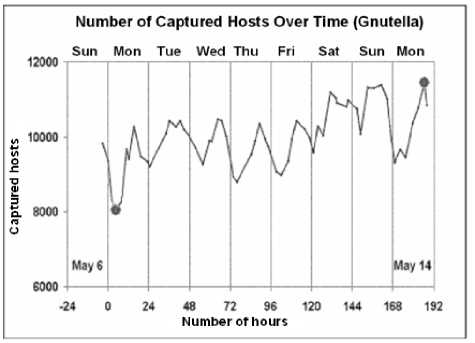
Figure 11: Statistical distribution of captured Gnutella peers

The data for configuring the underlying communication network, as well as other important parameters, have been taken from statistical investigations on the Internet, carried out at the University of Washington in the context of studies on peer-to-peer file sharing [30, 29] (see Figure 11). This information has been used to estimate the delay of operations performed by the TCP protocol and also the statistical distribution of queries over time. The total delay is structured as follows:

• Queue Delay, depending on the degree of congestion of the network and the size of the involved Queue;

• Processing Delay, given by the time required for: creating messages and decomposing/recomposing them into/from packets, and local query execution. It has been assumed that it takes $10^{-6}$ seconds to process one packet, and that a disk access takes 6 milliseconds (ms).

• Packet Transmission Delay, proportional to the size of the packet and the bandwidth;

• Propagation Delay, this is the network latency.

In order to measure the network latency we have used the estimations done on the Gnutella network, given by the RTT (round-trip time) of a 40-byte TCP packet exchanged between a peer and the measurement host. In particular, we have used the following distribution:

• 20% of peers have a latency smaller than 70 ms;

• 20% of peers have a latency higher than 280 ms;

• the remaining 60% of peers have latency uniformly distributed in between 70 and 280 ms.

Also to estimate the network bandwidth we have relied on the measurements done on Gnutella, according to which 78% of the users are connected on a large bandwidth (Cable, DSL, T1 or T3); according to the same estimation, about 30% of the users have a connection bandwidth higher than 3Mbps.

The size of the network was chosen to be 11400 sources, which is the maximum number of simultaneously connected peers in Gnutella over a continuous period of 192 hours.

The number of servers utilized for CCD, CDR and DCR approaches is 57, that is 0.5% of the total number of sources. Clearly, all the servers store the same network taxonomy or interpretation (or both).

In order to obtain the taxonomy, interpretation, and articulations of each source, the following parameters have been used, all with a uniform distribution:

• the size of the terminology is between 1 and 500 terms;

• the size of the interpretation of any term is between 1 and 100 objects;

• every source is articulated with 1 to 4 other sources;

• the size of a local taxonomy is 25% the size of the corresponding terminology;

• the total number of articulations is 6% of the size of the network terminology.

We have assumed that objects are URLs. This is typical in P2P networks. Following [20], the average size of a URL is 63.4 bytes. The size of the internal representation of a term is assumed to be the minimum amount of space required to uniquely identify an object within a set (the terminology where the term belongs) on a network of sources, each identified by an IP number. Finally, the values of the time-out are as follows: answer time-out (the time a source waits for an answer to arrive) is 60 seconds, while the cache time-out (the time a source keeps an answer in the Cache for re-use) is 600 seconds.

Most of these parameters are configurable.

5.2 The simulation experiments

In each experiment, the following variables have been measured:

• the time required to evaluate a query;

• the number of evaluated queries, required to compute the average response time;

• the size of the query result;

• the number of packets transmitted, including the packets exchanged for the ping-pong protocol, which has been used for inter-source communication;

• the number of visited sources.

For every approach, we have run a simulation experiment for the amount of time required to obtain a stable value for the response time. Each query is characterized by the following attributes:

• an integer number that identifies the query;

• the id of the source that formulates the query, randomly chosen in the interval [1, 11400];

• a set of terms randomly chosen from the terminology of the selected source, to be understood as a conjunction;

• the time at which the query is issued.

The query distribution is obtained from the statistical distribution of connected peers reported in Figure 11. In particular, the number of queries per unit of time is directly proportional to the number of connected peers. Since the same random generators have been used in all experiments for generating the query parameters, the same query distribution is used in each experiment.

In order to reduce the size of the required storage, we have gathered statistics for periods of 5 minutes. The average response time was divided by the size of the result; it was considered to be stable when the difference between the values for 3 consecutive periods of 5 minutes, equivalent to 15 minutes of simulated time, was less that $10^{-2}$ milliseconds. The goodness of this choice is confirmed by the low value of the standard deviation for all evaluated methods.

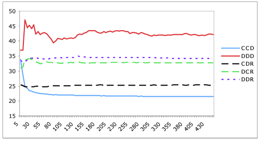
Figure 12: Average response time (milliseconds) per simulated time (minutes)

5.3 Results and discussion

Figure 12 details the distribution of the average response time in time for each method. As this Figure and Table 4 show, the fastest method is not surprisingly CCD, that is direct evaluation when both taxonomy and interpretation are centralized. Perhaps more surprisingly, the next best method is CDR, for reasons that will be analyzed below. As expected, the worst method is DDD, which does not allow any type of optimization, and at each step of the execution algorithm sends all collected terms and objects. The performance of the DCR and DDR methods tend to be the same, the former being slightly better because it can count on a centralized interpretation.

Needless to say, the actual values of the measured variables are determined also by the parameters chosen to configure the simulator, detailed above. What really matters are the relative values between the 5 compared methods, or in other words, the ranking of the methods produced by the experiment.

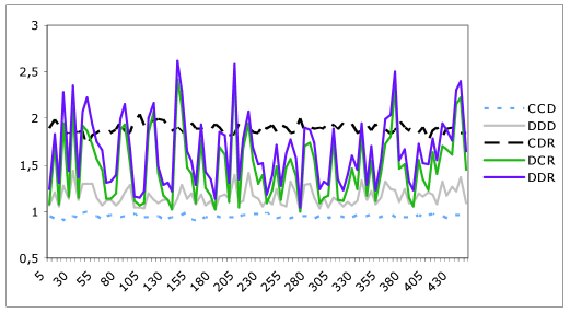
Figure 13: Average number of visited sources per simulated time (minutes)

In order to verify the correctness of the results, for every pair of measured variables the correlation coefficient has been computed. Correlation has been confirmed between:

• number of generated sub-queries and the number of exchanged messages,

• number of exchanged messages and number of visited sources.

In contrast, the number of exchanged messages and the size of the answer are independent.

The average number of sources visited for evaluating one query is reported in Figure 13. The queries that either addressed the terminologies of sources with no articulations or could be answered using the Cache, were evaluated locally, and therefore considered to visit no sources. This explains why the numbers in Figure 13 are so low, CCD being almost everywhere below 1. As it can be seen, re-writing methods are those involving a higher number of visits, with DDR having the highest for obvious reasons. Not surprisingly, CCD is the method requiring the least number of visits of all. However, the graphic suggests another clustering: the methods in which the taxonomy is distributed have similar, very irregular curves, whilst those in which the taxonomy is centralized have similar, much more regular curves. This explains why CDR is the second best method after CCD: the centralization of the taxonomy allows to re-write the query by contacting at most one source, the taxonomy server; if instead the taxonomy is distributed, several sources may need to be contacted in the re-writing stage, with the possibility that the same source be contacted more than once, if articulations require so. The distribution of the interpretation may require to contact several sources for the second stage, but the fact that this second stage is optimized implies that every involved source is contacted exactly once, and this makes this step affordable, so that on average 2 sources need to be visited, with a very small standard deviation (in fact, for CDR the average number of visited source is 1.887, and the standard deviation is 0.053).

This is confirmed by the number of exchanged messages (Figure 14). As expected the methods in which the taxonomy is distributed are those which require more message exchanges, with DDR being the worse due to the fact that also interpretations are distributed and the re-writing approach is followed. Also in this case CDR, although very similar to DDR, does much better, up to being not significantly different from the best method CCD.

Thus we can conclude that CDR is superior to all other distributed approaches because the optimization taking place between the 2 stages of the re-writing compensates the fact that more than one source needs to be contacted due to the distribution of the interpretations. In other words, distributing the taxonomy affects the performance of the method in a significant way, whilst optimization can compensate the distribution of the interpretations.

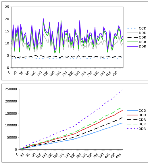
Figure 14: Average (top) and total (bottom) number of exchanged messages per simulated time (minutes)

6 Related work

In this Section we relate our work with the literature on peer-to-peer systems and data integration, with emphasis on the former. Some parts of the work reported in this paper have been already published. Namely, [36] presents a first model of a network of articulated sources, while [35] studies query evaluation on taxonomies including only term-to-term subsumption relationships. Finally, [26] introduced Qe(without proving its soundness and completeness), and gives hardness results for language extensions.

Description of our work in relation with P2P systems

A peer-to-peer (P2P) system is a distributed system in which participants (the peers) rely on one another for service, rather than solely relying on dedicated and often centralized servers. The most popular P2P systems have focused on specific application domains like music file sharing [3, 1, 2]) or on providing file-system-like capabilities [9]. In most of the cases, these systems do not provide semantic-based retrieval services as the name of an object (e.g. the title of a music file) is the only means for describing the object contents.

In our work, we make a distinction between the logical model of a network (presented in Section 2) and the architecture for implementing this model, which may be considered as a physical model of the network. Typically, this distinction is not made in the literature on P2P systems, thus we can compare only our pure P2P architecture, i.e. DDD, with the P2P literature.

In the DDD approach, in order to evaluate a query $q$ posed to a peer $\mathcal{S}$, the incoming query (which is always expressed over its own taxonomy) is propagated only to those peers to which $\mathcal{S}$ has an articulation, and which can therefore contribute to the answer of the query (the latter is determined by the taxonomy and the articulations of $\mathcal{S}$). Specifically, it is not the original query to be propagated, but a set of term sub-queries, each one belonging to the terminology of the recipient peer. Note that in DDD there is not any form of centralized index (like in Napster [3]), nor any flooding of queries (like in Gnutella [1]), nor any form of partitioned global index (like in Chord [33] and CAN [28]). Instead, we have a query propagation mechanism that is query- and articulation-dependent (note that Semantic Overlay Networks [13] is a very simplistic approach to this). Moreover note that the peers of our DDD model are quite autonomous in the sense that they do not have to share or publish their stored objects, taxonomies or mappings with the rest of the peers (neither to one central server, nor to the on-line peers). To participate in the network, a peer just has to answer the incoming queries by using its local base, and to propagate queries to those peers that according to its “knowledge” (i.e. taxonomy + articulations) may contribute to the evaluation of the query. However both of the above tasks are optional and at the “will” of the peer.

From a data modeling point of view several approaches for P2P systems have been proposed recently, including relational-based approaches [8], XML-based approaches [22] and RDF-based [27]. In this paper we consider the fully heterogeneous conceptual model approach (where each peer can have its own schema), with the only restriction that each conceptual model is represented as a taxonomy. A taxonomy can range from a simple tree-structured hierarchy of terms, to the concept lattice derived by Formal Concept Analysis [19], or to the concept lattice of a Description Logics theory. This taxonomy-based conceptual modeling approach has three main advantages (for more see [36]): (a) it is very easy to create the conceptual model of a source, (b) the integration of information from multiple sources can be done easily, and (c) automatic articulation using data-driven methods (like the one presented in [34]) are possible.

Recently, there have been several works on P2P systems endowed with logic-based models of the peers’ information bases and of the mappings relating them (called P2P mappings). These works can be classified in 2 broad categories: (1) those assuming propositional or Horn clauses as representation language or as a computational framework, and (2) those based on more powerful formalisms. With respect to the former category (e.g., see [6, 7, 5]), our work makes an important contribution, by providing a much simpler algorithm for performing query answering than those based on resolution. Indeed, we do rely on the theory of propositional Horn clauses, but only for proving the correctness of our algorithm. For implementing query evaluation, we devise an algorithm that avoids the (unnecessary) algorithmic complications that plague the methods based on resolution. As an example, after appropriate transformations our framework can be seen as a special case of that in [7]. Then, query evaluation can be performed by first computing the prime implicates of the negation of each term in the query, using the resolution-based algorithms presented in [7]. As the complexity of this problem is exponential w.r.t the size of the taxonomy and polynomial w.r.t. the size of $\mathit{Obj},$ there is no computational gain in using this approach. Instead, there is an algorithmic loss, since the method is much more complicated than ours.

As for the second category above, works in this area have focused on providing highly expressive knowledge representation languages in order to capture at once the widest range of applications. Notably, [12] proposes a model allowing, among other things, for existential quantification both in the bodies and in the heads of the mapping rules. Inevitably, such languages pose computational problems: deciding membership of a tuple in the answer of a query is undecidable in the framework proposed by [12], while disjunction in the rules’ heads makes the same problem coNP-hard already for datalog with unary predicate (i.e. terms). These problems are circumvented in both approaches by changing the semantics of a P2P network, in particular by adopting an epistemic reading of mappings. As a result, the inferential relation of the resulting logic is weakened up to the point of making the above mentioned decision problem solvable in polynomial time. In contrast, our approach aims at reaching the same goal (efficient support for P2P information access), but from a different standpoint: in particular, we achieve efficiency of the network query evaluation by limiting the expressiveness of the language for representing mappings (articulations, in our terminology), while retaining a classical Tarskian semantics of these mappings (seen as logical formulae). In other words, we aim at a smaller class of applications, but for this we offer a framework resting on the classical logical foundations. The complementarity of the two approaches is therefore evident. Since we have also shown [26], [35] that classical semantics leads to intractability as soon as the expressiveness of the mapping language is increased, we can say that we have covered a large part of our side of the trade-off.

In [10], a query answering algorithm for simple P2P systems is presented where each peer $\mathcal{S}$ is associated with a local database, an (exported) peer schema, and a set of local mapping rules from the schema of the local database to the peer schema. P2P mapping rules are of the form $cq_{1}\leadsto cq_{2}$, where $cq_{1},cq_{2}$ are conjunctive queries of the same arity $n\geq 1$ (possibly involving existential variables), expressed over the union of the schemata of the peers, and over the schema of a single peer, respectively. Note that this representation framework partially subsumes our network source framework, since in our case $cq_{1},cq_{2}$ are of arity 1, $cq_{1}$ is a conjunctive query of the form $u_{1}(x)\wedge\ldots\wedge u_{r}(x)$ over the terminology of a single peer and $q_{2}$ is a single atom query $t(x)$ over the terminology of the peer that the mapping (articulation) belongs to. However, simple P2P systems cannot express the local to a peer $\mathcal{S}$ taxonomy $\preceq_{\mathcal{S}}$ of our framework. Query answering in simple P2P systems according to the first-order logic (FOL) semantics is in general undecidable. Therefore, the authors adopt a new semantics based on epistemic logic in order to get decidability for query answering. Notably, the FOL semantics and epistemic logic semantics for our framework coincide. In particular, in [10], a centralized bottom-up algorithm is presented which essentially constructs a finite database $RDB$ which constitutes a “representative” of all the epistemic models of the P2P system. The answers to a conjunctive query $q$ are the answers of $q$ w.r.t. $RDB$. However, though this algorithm has polynomial time complexity, it is centralized and it suffers from the drawbacks of bottom-up computation that does not take into account the structure of the query.

The work in [10] is extended in [12], where a more general framework for P2P systems is considered, which fully subsumes our framework and whose semantics is based on epistemic logic. In particular, in [12], a peer is also associated with a set of (function-free) FOL formulas over the schema of the peer. A top-down distributed query answering algorithm is presented which is based on synchronous messaging. Essentially, the algorithm returns to the peer where the original query is posed, a datalog program by transferring the full extensions of the relevant to the query, peer source predicates along the paths of peers involved in query processing. The returned datalog program is used for providing the answers to the query. Obviously, our algorithm has computational advantages w.r.t. the algorithm in [12], since during query evaluation only the full or partial answer to a term (sub)query is transferred to the peer that posed the (sub)query, and not the full extensions of all terms involved in its evaluation.

The framework in [31], extends our framework by considering (i) $n$-ary (instead of unary) predicates (i.e. P2P mappings are general datalog rules) and (ii) a set of domain relations (also suggested in [32]), mapping the objects of one peer to the objects of another peer. A distributed query answering algorithm is presented based on synchronous messaging. However, the algorithm will perform poorly in our restricted framework, since when a peer receives a (sub)query, it iterates through the relevant P2P mappings and for each one of them, sends a (sub)query to the appropriate peer (waiting for its answer), until fix-point is reached. In our case, when a peer receives a (sub)query, each relevant P2P mapping is considered just once and no iteration until fix-point is required.

A P2P framework similar to [10] is presented in [23], where query answering according to FOL semantics is investigated. Since in general, query answering is undecidable, the authors present a centralized algorithm (employed in the Piazza system [21]), which however is complete (the algorithm is always sound), only for the case that polynomial time complexity in query answering can be achieved. This includes the condition that inclusion P2P mappings are acyclic. However, such a condition severely restricts the modularity of the system. Note that our algorithm is sound and complete even in the case that there are cycles in the term dependency path and it always terminates. Thus, our framework allows placing articulations between peers without further checks. This is quite important, because the actual interconnections are not under the control of any actor in the system.

In [17, 16], the authors consider a framework where each peer is associated with a relational database, and P2P mapping rules contain conjunctive queries in both the head and the body of the rule (possibly with existential variables), each expressed over the alphabet of a single peer. Again the semantics of the system is defined based on epistemic logic [15]. In these papers, a peer database update algorithm is provided allowing for subsequent peer queries to be answered locally without fetching data from other nodes at query time. The algorithm (which is based on asynchronous messaging) starts at the peer which sends queries to all neighbour peers according to the involved mapping rules. When a peer receives a query, the query is processed locally by the peer itself using its own data. This first answer is immediately replied back to the node which issued the query and sub-queries are propagated similarly to all neighbour peers. When a peer receives an answer, (i) it stores the answer locally, (ii) it materializes the view represented in the head on the involved mapping rule, and (ii) it propagates the result to the peer that issued the (sub)query. Answer propagation stops when no new answer tuples are coming to the peer through any dependency path, that is until fix-point is reached. In our case, the database update problem for a peer $\mathcal{S}$ amounts to invoking $\mathcal{S}^{\prime}:\textsc{Query}(q)$ for each articulation $q\preceq t$ from $\mathcal{S}$ to another peer $\mathcal{S}^{\prime}$ and storing the answer locally to $\mathcal{S}$. Note that our query answering algorithm is also based on asynchronous messaging. However, since it considers a limited framework, it is much simpler and no computation until fix-point is required. In particular, for each term (sub)query issued to a peer through ask, only one answer is returned through tell.

Relation with information integration

The literature about information integration distinguishes two main approaches: the local-as-view (LAV) and the global-as-view (GAV) approach (see [11, 25] for a comparison). In the LAV approach the contents of the sources are defined as views over the mediator’s schema, while in the GAV approach the mediator’s virtual contents are defined as views of the contents of the sources. The former approach offers flexibility in representing the contents of the sources, but query answering is “hard” because this requires answering queries using views ([14, 24, 37]). On the other hand, the GAV approach offers easy query answering (expansion of queries until getting to source relations), but the addition/deletion of a source implies updating the mediator view, i.e. the definition of the mediator relations. In our case, and if the articulations contain relationships between single terms, then we have the benefits of both GAV and LAV approaches, i.e. (a) the query processing simplicity of the GAV approach, as query processing basically reduces to unfolding the query using the definitions specified in the mapping, so as to translate the query in terms of accesses (i.e. queries) to the sources, and (b) the modeling scalability of the LAV approach, i.e. the addition of a new underlying source does not require changing the previous mappings. On the other hand, term-to-query articulations resemble the GAV approach.

7 Conclusions

In this paper, we have presented a model of networked information sources, each based on a different terminology and endowed with a taxonomy over that terminology, and logically connected to the other sources via articulations between respective concepts. The model is very flexible, in that it allows an articulation to connect a source to several other sources, by letting the terms in the tail of an articulation to be drawn from several terminologies.

For this kind of systems, we have presented a query evaluation procedure, rooted on an algorithm for testing the satisfiability of a set of propositional Horn clauses. Five architectures for implementing this procedure in a distributed setting have been considered, stemming from two orthogonal criteria: direct evaluation vs. query re-writing, and data allocation. For each of the resulting five interesting architectures, an implementation has been described, in terms of processes, communicating asynchronously through several queues. The design of the architectures and of the underlying communication scheme has emphasized efficiency and scalability.

The five implementations have been evaluated from a performance point of view, via simulations. A ranking has resulted from this evaluation, in which the direct evaluation over a client-server architecture (named CCD) overdoes the other ones, followed by the architecture in which the taxonomy is centralized and the queries are re-written before evaluation (named CDR).

Each implementation consists of several processes, each one implementing a complex algorithm. All these algorithms have been specified as UML state machines, in order to be simulated. For reasons of space, it has not been possible to give a complete account of all this work. In particular, more emphasis has been given to the implementations that perform best, CCD and CDR. However, upon request the complete set of UML state machines is available. Also the code of the simulator is available upon request.

We believe that the work presented in the paper provides conclusive knowledge on the addressed problem, and can be used to derive an engineered system to be put at work on real-word applications.

References

- [1] Gnutella(http://gnutella.wego.com).
- [2] Kazaa (http://www.kazaa.com/).
- [3] Napster (www.naptster.com), 2001.
- [4] K. Aberer, T. Catarci, P. Cudré-Mauroux, T. S. Dillon, S. Grimm, M. Hacid, A. Illarramendi, M. Jarrar, V. Kashyap, M. Mecella, E. Mena, E. J. Neuhold, A. M. Ouksel, T. Risse, M. Scannapieco, F. Saltor, L. De Santis, S. Spaccapietra, S. Staab, R. Studer, and O. De Troyer. “Emergent Semantics Systems”. In Procs. of the 1st Intern. IFIP Conference on Semantics of a Networked World (ICSNW 2004), pages 14–43, 2004.
- [5] P. Adjiman. Peer-to-Peer reasoning in propositional logic: algorithms, scalability, study and applications. PhD thesis, University of Paris South, 2006.
- [6] P. Adjiman, P. Chatalic, F. Goasdoué, M.-C. Rousset, and L. Simon. Distributed reasoning in a peer-to-peer setting. In R. L. de M ntaras and L. Saitta, editors, Proceedings of ECAI 2004, the European Conference on Artificial Intelligence, pages 945–946, Valencia, Spain, 2004. Short paper.
- [7] P. Adjiman, P. Chatalic, F. Goasdoué, M.-C. Rousset, and L. Simon. Distributed reasoning in a peer-to-peer setting: Application to the semantic web. Journal of Artificial Intelligence Research, 25:269–314, 2006.
- [8] Philip A. Bernstein, F. Giunchiglia, A. Kementsietsidis, J. Mylopoulos, L. Serafini, and I. Zaihrayeu. “Data Management for Peer-to-Peer Computing: A Vision”. In Proceedings of WebDB02, Madison, Wisconsin, June 2002.
- [9] W. J. Bolosky, J. R. Douceur, D. Ely, and M. Theimer. “Feasibility of a Serveless Distributed File System Deployed on an Existing Set of Desktop PCs”. In Proceedings of Measurement and Modeling of Computer Systems, June 2000.
- [10] Diego Calvanese, Elio Damaggio, Giuseppe De Giacomo, Maurizio Lenzerini, and Riccardo Rosati. “Semantic Data Integration in P2P Systems”. In Procs. of the First International Workshop on Databases, Information Systems and Peer-to-Peer Computing (DBISP2P 2003), pages 79–90, 2003.
- [11] Diego Calvanese, Giuseppe De Giacomo, and Maurizio Lenzerini. “A Framework for Ontology Integration”. In Proc. of the 2001 Int. Semantic Web Working Symposium (SWWS 2001), pages 303–316, Stanford University, California, USA, July 30 - August 1 2001.
- [12] Diego Calvanese, Giuseppe De Giacomo, Maurizio Lenzerini, and Riccardo Rosati. “Logical foundations of peer-to-peer data integration”. In Procs. of the 23rd ACM symposium on Principles of database systems, PODS’2004, pages 241–251, New York, NY, USA, 2004. ACM Press.
- [13] Arturo Crespo and Hector Garcia-Molina. “Semantic Overlay Networks for P2P Systems”. Technical report, Computer Science Department, Stanford University, October 2002.
- [14] Oliver M. Duschka and Michael R. Genesereth. Answering recursive queries using views. In Procs. of the 16th ACM SIGACT-SIGMOD-SIGART Symposium on Principles of Database Systems (PODS’97), pages 109–116, Tucson, Arizona, 12-14 May 1997.
- [15] E. Franconi, G. M. Kuper, A. Lopatenko, and L. Serafini. “A Robust Logical and Computational Characterisation of Peer-to-Peer Database Systems”. In Procs. of the First International Workshop on Databases, Information Systems, and Peer-to-Peer Computing (DBISP2P 2003), pages 64–76, 2003.
- [16] E. Franconi, G. M. Kuper, A. Lopatenko, and I. Zaihrayeu. “A Distributed Algorithm for Robust Data Sharing and Updates in P2P Database Networks”. In Procs. of the EDBT’04 Intern. Workshop on Peer-to-Peer Computing and Databases (P2P&DB 2004), pages 446–455, 2004.
- [17] E. Franconi, G. M. Kuper, A. Lopatenko, and I. Zaihrayeu. “Queries and Updates in the coDB Peer to Peer Database System”. In Procs. of the 30th International Conference on Very Large Data Bases (VLDB 2004), pages 1277–1280, 2004.
- [18] Giorgio Gallo, Giustino Longo, and Stefano Pallottino. “Directed Hypergraphs and Applications”. Discrete Applied Mathematics, 42(2):177–201, 1993.
- [19] Bernhard Ganter and Rudolf Wille. “Formal Concept Analysis: Mathematical Foundations”. Springer-Verlag, Heidelberg, 1999.
- [20] J. L. Giulleume, M. Latapy, and L. Viennot. Efficient and simple encodings for the web graph. In Proceedings of WAIM’02, the 3rd International Conference on Web-Age Information Management, 2002.
- [21] A. Y. Halevy, Z. G. Ives, J. Madhavan, P. Mork, D. Suciu, and I. Tatarinov. “The Piazza Peer Data Management System”. IEEE Transactions on Knowledge and Data Engineering, 16(7):787–798, 2004.
- [22] Alon Halevy, Zachary Ives, Peter Mork, and Igor Tatarinov. “Piazza: Data Management Infrastructure for Semantic Web Applications”. In Procs. of the 12th International Conference on World Wide Web (WWW 2003), pages 556 – 567, May 2003.
- [23] Alon Halevy, Zachary Ives, Dan Suciu, and Igor Tatarinov. “Schema Mediation in Peer Data Management Systems”. In Procs. of the 19th International Conference on Data Engineering (ICDE’03), pages 505–518, March 2003.
- [24] Alon Y. Halevy. “Answering Queries Using Views: A Survey”. VLDB Journal, 10(4):270–294, 2001.
- [25] Maurizio Lenzerini. “Data Integration: A Theoretical Perspective”. In Proc. of the 21st ACM SIGMOD-SIGACT-SIGART Symposium on Principles of Database Systems (PODS 2002), pages 233–246, Madison, Wisconsin, USA, June 2002.
- [26] Carlo Meghini and Yannis Tzitzikas. “Querying Articulated Sources”. In Procs. of the 3rd Intern. Conference on Ontologies, Databases and Applications of Semantics for Large Scale Information Systems, ODBASE’2004, pages 945–962, Larnaca, Cyprus, October 2004.
- [27] W. Nejdl, B. Wolf, C. Qu, S. Decker, M. Sintek, A. Naeve, M. Nilsson, M. Palmer, and T. Risch. ”EDUTELLA: A P2P networking infrastructure based on RDF”. In Procs. of the 11th International Conference on World Wide Web (WWW’02), pages 604 – 615, 2002.
- [28] Sylvia Ratnasamy, Paul Francis, Mark Handley, Richard Karp, and Scott Shenker. A scalable content addressable network. In Proceedings of the 2001 ACM SIGCOMM Conference, pages 161–172, 2001.
- [29] S. Saroiu, P. K. Gummadi, and S. D. Gribble. Estimating latency between arbitrary internet end hosts. In Proceedings of IMW 2002, the Second SIGCOMM Internet Measurement Workshop, Marseille, France, November 2002.
- [30] S. Saroiu, P. K. Gummadi, and S. D. Gribble. A measurement study of peer-to-peer file sharing systems. In Proceedings of MMCN 2002 Multimedia Computing and Networking, January 2002.
- [31] L. Serafini and C. Ghidini. “Using Wrapper Agents to Answer Queries in Distributed Information Systems”. In Procs. of the First International Conference on Advances in Information Systems (ADVIS ’00), pages 331–340. Springer-Verlag, 2000.
- [32] L. Serafini, F. Giunchiglia, J. Mylopoulos, and P. A. Bernstein. “Local Relational Model: A Logical Formalization of Database Coordination”. In Procs. of the 4th International and Interdisciplinary Conference on Modeling and Using Context(CONTEXT 2003), pages 286–299, 2003.
- [33] Ion Stoica, Robert Morris, David Karger, M. Frans Kaashoek, and Hari Balakrishnan. “Chord: A Scalable Peer-to-peer Lookup Service for Internet Applications”. In Proceedings of the 2001 ACM SIGCOMM Conference, 2001.
- [34] Yannis Tzitzikas and Carlo Meghini. “Ostensive Automatic Schema Mapping for Taxonomy-based Peer-to-Peer Systems”. In Seventh International Workshop on Cooperative Information Agents, CIA-2003, pages 78–92, Helsinki, Finland, August 2003. (Best Paper Award).
- [35] Yannis Tzitzikas and Carlo Meghini. “Query Evaluation in Peer-to-Peer Networks of Taxonomy-based Sources”. In Procs. of 19th Int. Conf. on Cooperative Information Systems, CoopIS’2003, pages 263–281, Catania, Sicily, Italy, November 2003.
- [36] Yannis Tzitzikas, Carlo Meghini, and Nicolas Spyratos. “Taxonomy-based Conceptual Modeling for Peer-to-Peer Networks”. In Procs. of 22th Int. Conf. on Conceptual Modeling, ER’2003, pages 446–460, Chicago, Illinois, October 2003.
- [37] Jeffrey D. Ullman. “Information integration using logical views”. In Procs. of the 6th Int. Conf. on Database Theory (ICDT-97), pages 19–40, Delphi, Greece, 8-10 January 1997.