On the formal statement of the special principle of relativity

Abstract

The aim of the paper is to develop a proper mathematical formalism which can help to clarify the necessary conceptual plugins to the special principle of relativity and leads to a deeper understanding of the principle in its widest generality.

1 Introduction

The aim of this paper is to spell out the (special) relativity principle (RP) in a precise mathematical form. There are various verbal formulations of the principle. In its shortest form it says that “All the laws of physics take the same form in any inertial frame of reference.” The laws of physics in a reference frame $K$ are meant to be the laws of physics as they are ascertained by an observer being at rest relative to the reference frame $K$; less anthropomorphically, as they appear in the results of the measurements, such that both the measuring equipments and the objects to be measured are co-moving with $K$.

For example, consider the following simple application of the principle in Einstein’s 1905 paper:

Let there be given a stationary rigid rod; and let its length be $l$ as measured by a measuring-rod which is also stationary. We now imagine the axis of the rod lying along the axis of $x$ of the stationary system of co-ordinates, and that a uniform motion of parallel translation with velocity $v$ along the axis of $x$ in the direction of increasing $x$ is then imparted to the rod. We now inquire as to the length of the moving rod, and imagine its length to be ascertained by the following two operations:

• The observer moves together with the given measuring-rod and the rod to be measured, and measures the length of the rod directly by superposing the measuring-rod, in just the same way as if all three were at rest.

• By means of stationary clocks set up in the stationary system and synchronizing in accordance with [the light-signal synchronization], the observer ascertains at what points of the stationary system the two ends of the rod to be measured are located at a definite time. The distance between these two points, measured by the measuring-rod already employed, which in this case is at rest, is also a length which may be designated “the length of the rod.”

In accordance with the principle of relativity the length to be discovered by the operation (a)—we will call it “the length of the rod in the moving system”—must be equal to the length $l$ of the stationary rod.

The length to be discovered by the operation (b) we will call “the length of the (moving) rod in the stationary system.” This we shall determine on the basis of our two principles, and we shall find that it differs from $l$. [all italics added]

Thus, with the following formulation (Szabó 2004) one can express in more detail how the principle is actually understood:

• The physical description of the behavior of a system co-moving as a whole with an inertial frame $K$, expressed in terms of the results of measurements obtainable by means of measuring equipments co-moving with $K$, takes the same form as the description of the similar behavior of the same system when it is co-moving with another inertial frame $K^{\prime}$, expressed in terms of the measurements with the same equipments when they are co-moving with $K^{\prime}$.

Our main concern in this paper is to unpack the verbal statement (RP) and to provide its general mathematical formulation. We are hopeful that the formalism we develop here helps to clarify the required conceptual plugins to the RP and leads to a deeper understanding of the principle in its widest generality.

2 The statement of the RP

Consider an arbitrary collection of physical quantities $\xi_{1},\xi_{2},\ldots\xi_{n}$ in $K$, operationally defined by means of some operations with some equipments being at rest in $K$. Let $\xi^{\prime}_{1},\xi^{\prime}_{2},\ldots\xi^{\prime}_{n}$ denote another collection of physical quantities that are defined by the same operations with the same equipments, but in different state of motion, namely, in which they are all moving with constant velocity $\mathbf{V}$ relative to $K$, co-moving with $K^{\prime}$. Since, for all $i=1,2,\ldots n$, both $\xi_{i}$ and $\xi^{\prime}_{i}$ are measured by the same equipment—although in different physical conditions—with the same pointer scale, it is plausible to assume that the possible values of $\xi_{i}$ and $\xi^{\prime}_{i}$ range over the same $\sigma_{i}\subseteq\mathbb{R}$. We introduce the following notation: $\Sigma={\displaystyle\times_{i=1}^{n}\sigma_{i}}\subseteq\mathbb{R}^{n}$.

It must be emphasized that quantities $\xi_{1},\xi_{2},\ldots\xi_{n}$ and $\xi^{\prime}_{1},\xi^{\prime}_{2},\ldots\xi^{\prime}_{n}$ are, a priori, different physical quantities, due to the fact that the operations by which the quantities are defined are performed under different physical conditions; with measuring equipments of different states of motion. Any objective (non-conventional) relationship between them must be a contingent law of nature. Thus, the same numeric values, say, $(5,12,\ldots 61)\in\mathbb{R}^{n}$ correspond to different states of affairs when $\xi_{1}=5,\xi_{2}=12,\ldots\xi_{n}=61$ versus $\xi^{\prime}_{1}=5,\xi^{\prime}_{2}=12,\ldots\xi^{\prime}_{n}=61$. Consequently, $\left(\xi_{1},\xi_{2},\ldots\xi_{n}\right)$ and $\left(\xi^{\prime}_{1},\xi^{\prime}_{2},\ldots\xi^{\prime}_{n}\right)$ are not elements of the same “space of physical quantities”; although the numeric values of the physical quantities, in both cases, can be represented in $\Sigma={\displaystyle\times_{i=1}^{n}\sigma_{i}}\subseteq\mathbb{R}^{n}$.

Mathematically, one can express this fact by means of two different $n$-dimensional manifolds, $\Omega$ and $\Omega^{\prime}$, each covered by one global coordinate system, $\phi$ and $\phi^{\prime}$ respectively, such that $\phi:\Omega\rightarrow\Sigma$ assigns to every point of $\Omega$ one of the possible $n$-tuples of numerical values of physical quantities $\xi_{1},\xi_{2},\ldots\xi_{n}$ and $\phi^{\prime}:\Omega^{\prime}\rightarrow\Sigma$ assigns to every point of $\Omega^{\prime}$ one of the possible $n$-tuples of numerical values of physical quantities $\xi^{\prime}_{1},\xi^{\prime}_{2},\ldots\xi^{\prime}_{n}$

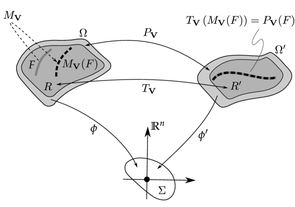
Figure 1: The relativity principle

(Fig. 1). In this way, a point $\omega\in\Omega$ represents the class of physical constellations in which the quantities $\xi_{1},\xi_{2},\ldots\xi_{n}$ take the values $\xi_{1}=\phi_{1}(\omega),\xi_{2}=\phi_{2}(\omega),\ldots\xi_{n}=\phi_{n}(\omega)$; similarly, a point $\omega^{\prime}\in\Omega^{\prime}$ represents the physical constellation characterized by $\xi^{\prime}_{1}=\phi^{\prime}_{1}(\omega^{\prime}),\xi^{\prime}_{2}=\phi^{\prime}_{2}(\omega^{\prime}),\ldots\xi^{\prime}_{n}=\phi^{\prime}_{n}(\omega^{\prime})$. Again, these physical constellations are generally different, even in case of $\phi(\omega)=\phi^{\prime}(\omega^{\prime})\in\mathbb{R}^{n}$.

In the above sense, the points of $\Omega$ and the points of $\Omega^{\prime}$ range over all possible value combinations of physical quantities $\xi_{1},\xi_{2},\ldots\xi_{n}$ and $\xi^{\prime}_{1},\xi^{\prime}_{2},\ldots\xi^{\prime}_{n}$. It might be the case however that some combinations are impossible, in the sense that they never come to existence in the physical world. Let us denote by $R\subseteq\Omega$ and $R^{\prime}\subseteq\Omega^{\prime}$ the physically admissible parts of $\Omega$ and $\Omega^{\prime}$. Note that $\phi(R)$ is not necessarily identical with $\phi^{\prime}(R^{\prime})$.

We shall use a bijection $P_{\mathbf{V}}:\Omega\rightarrow\Omega^{\prime}$ (“putting primes”; Bell 1987, p. 73) defined by means of the two coordinate maps $\phi$ and $\phi^{\prime}$:

$$P_{\mathbf{V}}\overset{{}^{def}}{=}\left(\phi^{\prime}\right)^{-1}\circ\phi$$ (1)

In contrast with $P_{\mathbf{V}}$, we now introduce the concept of what we call the “transformation” of physical quantities. It is conceived as a bijection

$$T_{\mathbf{V}}:\Omega\supseteq R\rightarrow R^{\prime}\subseteq\Omega^{\prime}$$ (2)

determined by the contingent fact that whenever a physical constellation belongs to the class represented by some $\omega\in R$ then it also belongs to the class represented by $T_{\mathbf{V}}(\omega)\in R^{\prime}$, and vice versa. Since $\xi_{1},\xi_{2},\ldots\xi_{n}$ can be various physical quantities in the various contexts, nothing guarantees that such a bijection exists. We assume however the existence of $T_{\mathbf{V}}$.

Remark 1.   It is worthwhile to consider several examples.

• Let $\left(\xi_{1},\xi_{2}\right)$ be $\left(p,T\right)$, the pressure and the temperature of a given (equilibrium) gas; and let $\left(\xi^{\prime}_{1},\xi^{\prime}_{2}\right)$ be $\left(p^{\prime},T^{\prime}\right)$, the pressure and the temperature of the same gas, measured by the moving observer in $K^{\prime}$. In this case, there exists a one-to-one $T_{\mathbf{V}}$:

  $$p^{\prime} = p$$ (3)

  $$T^{\prime} = T\gamma^{-1}$$ (4)

  where $\gamma=\left(1-\frac{V^{2}}{c^{2}}\right)^{-\frac{1}{2}}$ (Tolman 1949, pp. 158–159). A point $\omega\in\Omega$ of coordinates, say, $p=101325$ and $T=300$ (in units $Pa$ and ${}^{\circ}K$) represents the class of physical constellations—the class of possible worlds—in which the gas in question has pressure of $101325\,Pa$ and temperature of $300\,{}^{\circ}K$. Due to (4), this class of physical constellations is different from the one represented by $P_{\mathbf{V}}\left(\omega\right)\in\Omega^{\prime}$ of coordinates $p^{\prime}=101325$ and $T^{\prime}=300$; but it is identical to the class of constellations represented by $T_{\mathbf{V}}\left(\omega\right)\in\Omega^{\prime}$ of coordinates $p^{\prime}=101325$ and $T^{\prime}=300\gamma^{-1}$.

• Let $\left(\xi_{1},\xi_{2},\ldots\xi_{10}\right)$ be $\left(t,x,y,z,E_{x},E_{y},E_{z},r_{x},r_{y},r_{z}\right)$, the time, the space coordinates where the electric field strength is taken, the three components of the field strength, and the space coordinates of a particle. And let $\left(\xi^{\prime}_{1},\xi^{\prime}_{2},\ldots\xi^{\prime}_{10}\right)$ be $\left(t^{\prime},x^{\prime},y^{\prime},z^{\prime},E^{\prime}_{x},E^{\prime}_{y},E^{\prime}_{z},r^{\prime}_{x},r^{\prime}_{y},r^{\prime}_{z}\right)$, the similar quantities obtainable by means of measuring equipments co-moving with $K^{\prime}$. In this case, there is no suitable one-to-one $T_{\mathbf{V}}$, as the electric field strength in $K$ does not determine the electric field strength in $K^{\prime}$, and vice versa.

• Let $\left(\xi_{1},\xi_{2},\ldots\xi_{13}\right)$ be $\left(t,x,y,z,E_{x},E_{y},E_{z},B_{x},B_{y},B_{z},r_{x},r_{y},r_{z}\right)$ and let $\left(\xi^{\prime}_{1},\xi^{\prime}_{2},\ldots\xi^{\prime}_{13}\right)$ be $\left(t^{\prime},x^{\prime},y^{\prime},z^{\prime},E^{\prime}_{x},E^{\prime}_{y},E^{\prime}_{z},B^{\prime}_{x},B^{\prime}_{y},B^{\prime}_{z},r^{\prime}_{x},r^{\prime}_{y},r^{\prime}_{z}\right)$, where $B_{x},B_{y},B_{z}$ and $B^{\prime}_{x},B^{\prime}_{y},B^{\prime}_{z}$ are the magnetic field strengths in $K$ and $K^{\prime}$. In this case, in contrast with (b), the well known Lorentz transformations of the spatio-temporal coordinates and the electric and magnetic field strengths constitute a proper one-to-one $T_{\mathbf{V}}$. $\lrcorner$

Next we turn to the general formulation of the concept of the description of a particular behavior of a physical system, say, in $K$. We are probably not far from the truth if we assume that such a description is, in its most abstract sense, a relation between physical quantities $\xi_{1},\xi_{2},\ldots\xi_{n}$; in other words, it can be given as a subset $F\subset R$.

Remark 2.   Consider the above example (a) in Remark 2. An isochoric process of the gas can be described by the subset $F$ that is, in coordinates, determined by the following single equation:

$$F\,\,\,\left\{p=\kappa T\right.$$ (5)

with a certain constant $\kappa$.

To give another example, consider the case (b). The relation $F$ given by equations

$$F\,\,\,\left\{\begin{aligned} E_{x}&=E_{0}\\ E_{y}&=0\\ E_{z}&=0\\ r_{x}&=x_{0}+v_{0}t\\ r_{y}&=0\\ r_{z}&=0\end{aligned}\right.$$ (6)

with some specific values of $E_{0},x_{0},v_{0}$ describes a neutral particle moving with constant velocity in a static homogeneous electric field. $\lrcorner$

Of course, one may not assume that an arbitrary relation $F\subset R$ has physical meaning. Let $\mathcal{E}\subset 2^{R}$ be the set of those $F\subset R$ which describe a particular behavior of the system. We shall call $\mathcal{E}$ the set of equations describing the physical system in question. The term is entirely justified. In practical calculations, two systems of equations are regarded to be equivalent if and only if they have the same solutions. Therefore, a system of equations can be identified with the set of its solutions. In general, the equations can be algebraic equations, ordinary and partial integro-differential equations, linear and nonlinear, whatever. So, in its most abstract sense, a system of equations is a set of subsets of $R$.

Now, consider the following subsets of $\Omega^{\prime}$, determined by an $F\in\mathcal{E}$:

• which formally is the “primed $F$”, that is a relation of exactly the same “form” as $F$, but in the primed variables $\xi^{\prime}_{1},\xi^{\prime}_{2},\ldots\xi^{\prime}_{n}$. Note that relation $P_{\mathbf{V}}(F)$ does not necessarily describe a true physical situation, as it can be not realized in nature.

• which is the same description of the same physical situation as $F$, but expressed in the primed variables.

We need one more concept. The RP is about the connection between two situations: one is in which the system, as a whole, is at rest relative to inertial frame $K$, the other is in which the system shows the similar behavior, but being in a collective motion relative to $K$, co-moving with $K^{\prime}$. In other words, we assume the existence of a map $M_{\mathbf{V}}:\,\mathcal{E}\rightarrow\mathcal{E}$, assigning to each $F\in\mathcal{E}$, stipulated to describe the situation in which the system is co-moving as a whole with inertial frame $K$, another relation $M_{\mathbf{V}}(F)\in\mathcal{E}$, describing the similar behavior of the same system when it is, as a whole, co-moving with inertial frame $K^{\prime}$, that is, when it is in a collective motion with velocity $\mathbf{V}$ relative to $K$.

Now, applying all these concepts, what the RP states is the following:

$$T_{\mathbf{V}}\left(M_{\mathbf{V}}(F)\right)=P_{\mathbf{V}}(F)\,\,\,\,\mbox{ for all }F\in\mathcal{E}$$ (7)

or equivalently,

$$P_{\mathbf{V}}(F)\subset R^{\prime}\mbox{ and }M_{\mathbf{V}}(F)=T_{\mathbf{V}}^{-1}\left(P_{\mathbf{V}}(F)\right)\,\,\,\,\mbox{ for all }F\in\mathcal{E}$$ (8)

Remark 3.   Notice that, for a given fixed $F$, everything on the right hand side of the equation in (8), $P_{\mathbf{V}}$ and $T_{\mathbf{V}}$, are determined only by the physical behaviors of the measuring equipments when they are in various states of motion. In contrast, the meaning of the left hand side, $M_{\mathbf{V}}(F)$, depends on the physical behavior of the object physical system described by $F$ and $M_{\mathbf{V}}(F)$, when it is in various states of motion. That is to say, the two sides of the equation reflect the behaviors of different parts of the physical reality; and the RP expresses a law-like regularity between the behaviors of these different parts. $\lrcorner$

Remark 4.   Let us illustrate these concepts with a well-known textbook example of a static versus uniformly moving charged particle. The static field of a charge $q$ being at rest at point $(x_{0},y_{0},z_{0})$ in $K$ is the following:

$$F\,\,\,\left\{\begin{aligned} E_{x}&=\frac{q\left(x-x_{0}\right)}{\left(\left(x-x_{0}\right)^{2}+\left(y-y_{0}\right)^{2}+\left(z-z_{0}\right)^{2}\right)^{\nicefrac{{3}}{{2}}}}\\ E_{y}&=\frac{q\left(y-y_{0}\right)}{\left(\left(x-x_{0}\right)^{2}+\left(y-y_{0}\right)^{2}+\left(z-z_{0}\right)^{2}\right)^{\nicefrac{{3}}{{2}}}}\\ E_{z}&=\frac{q\left(z-z_{0}\right)}{\left(\left(x-x_{0}\right)^{2}+\left(y-y_{0}\right)^{2}+\left(z-z_{0}\right)^{2}\right)^{\nicefrac{{3}}{{2}}}}\\ B_{x}&=0\\ B_{y}&=0\\ B_{z}&=0\end{aligned}\right.$$ (9)

The stationary field of a charge $q$ moving at constant velocity $\mathbf{V}=\left(V,0,0\right)$ relative to $K$ can be obtained by solving the equations of electrodynamics (in $K$) with the time-depending source (for example, Jackson 1999, pp. 661–665):

$$M_{\mathbf{V}}(F)\,\,\,\left\{\begin{aligned} E_{x}&=\frac{qX_{0}}{\left(X_{0}^{2}+\left(y-y_{0}\right)^{2}+\left(z-z_{0}\right)^{2}\right)^{\nicefrac{{3}}{{2}}}}\\ E_{y}&=\frac{\gamma q\left(y-y_{0}\right)}{\left(X_{0}^{2}+\left(y-y_{0}\right)^{2}+\left(z-z_{0}\right)^{2}\right)^{\nicefrac{{3}}{{2}}}}\\ E_{z}&=\frac{\gamma q\left(z-z_{0}\right)}{\left(X_{0}^{2}+\left(y-y_{0}\right)^{2}+\left(z-z_{0}\right)^{2}\right)^{\nicefrac{{3}}{{2}}}}\\ B_{x}&=0\\ B_{y}&=-c^{-2}VE_{z}\\ B_{z}&=c^{-2}VE_{y}\end{aligned}\right.$$ (10)

where where $(x_{0},y_{0},z_{0})$ is the initial position of the particle at $t=0$, $X_{0}=\gamma\left(x-\left(x_{0}+Vt\right)\right)$.

Now, we form the same expressions as (9) but in the primed variables of the co-moving reference frame $K^{\prime}$:

$$P_{\mathbf{V}}\left(F\right)\,\,\,\left\{\begin{aligned} E^{\prime}_{x}&=\frac{q^{\prime}\left(x^{\prime}-x^{\prime}_{0}\right)}{\left(\left(x^{\prime}-x^{\prime}_{0}\right)^{2}+\left(y^{\prime}-y^{\prime}_{0}\right)^{2}+\left(z^{\prime}-z^{\prime}_{0}\right)^{2}\right)^{\nicefrac{{3}}{{2}}}}\\ E^{\prime}_{y}&=\frac{q^{\prime}\left(y^{\prime}-y^{\prime}_{0}\right)}{\left(\left(x^{\prime}-x^{\prime}_{0}\right)^{2}+\left(y^{\prime}-y^{\prime}_{0}\right)^{2}+\left(z^{\prime}-z^{\prime}_{0}\right)^{2}\right)^{\nicefrac{{3}}{{2}}}}\\ E^{\prime}_{z}&=\frac{q^{\prime}\left(z^{\prime}-z^{\prime}_{0}\right)}{\left(\left(x^{\prime}-x^{\prime}_{0}\right)^{2}+\left(y^{\prime}-y^{\prime}_{0}\right)^{2}+\left(z^{\prime}-z^{\prime}_{0}\right)^{2}\right)^{\nicefrac{{3}}{{2}}}}\\ B^{\prime}_{x}&=0\\ B^{\prime}_{y}&=0\\ B^{\prime}_{z}&=0\end{aligned}\right.$$ (11)

By means of the Lorentz transformation rules of the space-time coordinates, the field strengths and the electric charge (e.g. Tolman 1949), one can express (11) in terms of the original variables of $K$:

$$T_{\mathbf{V}}^{-1}\left(P_{\mathbf{V}}(F)\right)\,\,\,\left\{\begin{aligned} E_{x}&=\frac{qX_{0}}{\left(X_{0}^{2}+\left(y-y_{0}\right)^{2}+\left(z-z_{0}\right)^{2}\right)^{\nicefrac{{3}}{{2}}}}\\ E_{y}&=\frac{\gamma q\left(y-y_{0}\right)}{\left(X_{0}^{2}+\left(y-y_{0}\right)^{2}+\left(z-z_{0}\right)^{2}\right)^{\nicefrac{{3}}{{2}}}}\\ E_{z}&=\frac{\gamma q\left(z-z_{0}\right)}{\left(X_{0}^{2}+\left(y-y_{0}\right)^{2}+\left(z-z_{0}\right)^{2}\right)^{\nicefrac{{3}}{{2}}}}\\ B_{x}&=0\\ B_{y}&=-c^{-2}VE_{z}\\ B_{z}&=c^{-2}VE_{y}\end{aligned}\right.$$ (12)

We find that the result is indeed the same as (10) describing the field of the moving charge: $M_{\mathbf{V}}(F)=T_{\mathbf{V}}^{-1}\left(P_{\mathbf{V}}(F)\right)$. That is to say, the RP seems to be true in this particular case.

Reversely, assuming that the particle + electromagnetic field system satisfies the RP, that is, (8) holds for the equations of electrodynamics, one can derive the stationary field of a uniformly moving point charge (10) from the static field (9). $\lrcorner$

3 Covariance

Now we have a strict mathematical formulation of the RP for a physical system described by a system of equations $\mathcal{E}$. Remarkably, however, we still have not encountered the concept of “covariance” of equations $\mathcal{E}$. The reason is that the RP and the covariance of equations $\mathcal{E}$ are not equivalent—in contrast to what many believe. In fact, the logical relationship between the two conditions is much more complex. To see this relationship in more detail, we previously need to clarify a few things.

Consider the following two sets: $P_{\mathbf{V}}(\mathcal{E})=\{P_{\mathbf{V}}(F)|F\in\mathcal{E}\}$ and $T_{\mathbf{V}}(\mathcal{E})=\{T_{\mathbf{V}}(F)|F\in\mathcal{E}\}$. Since a system of equations can be identified with its set of solutions, $P_{\mathbf{V}}(\mathcal{E})\subset 2^{\Omega^{\prime}}$ and $T_{\mathbf{V}}(\mathcal{E})\subset 2^{R^{\prime}}$ can be regarded as two systems of equations for functional relations between $\xi^{\prime}_{1},\xi^{\prime}_{2},\ldots\xi^{\prime}_{n}$. In the primed variables, $P_{\mathbf{V}}(\mathcal{E})$ has “the same form” as $\mathcal{E}$. Nevertheless, it can be the case that $P_{\mathbf{V}}(\mathcal{E})$ does not express a true physical law, in the sense that its solutions do not necessarily describe true physical situations. In contrast, $T_{\mathbf{V}}(\mathcal{E})$ is nothing but $\mathcal{E}$ expressed in variables $\xi^{\prime}_{1},\xi^{\prime}_{2},\ldots\xi^{\prime}_{n}$.

Now, covariance intuitively means that equations $\mathcal{E}$ “preserve their forms against the transformation $T_{\mathbf{V}}$”. That is, in terms of the formalism we developed:

$$T_{\mathbf{V}}(\mathcal{E})=P_{\mathbf{V}}(\mathcal{E})$$ (13)

or, equivalently,

$$P_{\mathbf{V}}(\mathcal{E})\subset 2^{R^{\prime}}\,\mbox{ and }\,\mathcal{E}=T_{\mathbf{V}}^{-1}\left(P_{\mathbf{V}}(\mathcal{E})\right)$$ (14)

The first thing we have to make clear is that—even if we know or presume that it holds—covariance (14) is obviously not sufficient for the RP (8). For, (14) only guarantees the invariance of the set of solutions, $\mathcal{E}$, against $T_{\mathbf{V}}^{-1}\circ P_{\mathbf{V}}$ , but it says nothing about which solution of $\mathcal{E}$ corresponds to which solution. In Bell’s words:

Lorentz invariance alone shows that for any state of a system at rest there is a corresponding ‘primed’ state of that system in motion. But it does not tell us that if the system is set anyhow in motion, it will actually go into the ’primed’ of the original state, rather than into the ‘prime’ of some other state of the original system. (Bell 1987, p. 75)

While it is the very essence of the RP that the solution $M_{\mathbf{V}}(F)$, describing the system in motion relative to $K$, corresponds to solution $T_{\mathbf{V}}^{-1}\circ P_{\mathbf{V}}(F)$. For example, what we use in the above mentioned textbook derivation of the stationary electromagnetic field of a uniformly moving point charge (end of Remark 2) is not the covariance of the equations—that would be not enough—but statement (8), that is, what the RP claims about the solutions of the equations in detail.

In a precise sense, covariance is not only not sufficient for the RP, but it is not even necessary

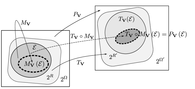
Figure 2: The RP only implies that $T_{\mathbf{V}}(\mathcal{E})\supseteq T_{\mathbf{V}}\circ M_{\mathbf{V}}\left(\mathcal{E}\right)=P_{\mathbf{V}}\left(\mathcal{E}\right)$. Covariance of $\mathcal{E}$ would require that $T_{\mathbf{V}}(\mathcal{E})=P_{\mathbf{V}}(\mathcal{E})$, which is generally not the case

(Fig. 2). The RP only implies that

$$T_{\mathbf{V}}(\mathcal{E})\supseteq T_{\mathbf{V}}\left(M_{\mathbf{V}}\left(\mathcal{E}\right)\right)=P_{\mathbf{V}}\left(\mathcal{E}\right)$$ (15)

(7) implies (13) only if we have the following extra condition:

$$M_{\mathbf{V}}\left(\mathcal{E}\right)=\mathcal{E}$$ (16)

4 Initial and boundary conditions

Let us finally consider the situation when the solutions of a system of equations $\mathcal{E}$ are specified by some extra conditions—initial and/or boundary value conditions, for example. In our general formalism, an extra condition for $\mathcal{E}$ is a system of equations $\psi\subset 2^{\Omega}$ such that there exists exactly one solution $\left[\psi\right]_{\mathcal{E}}$ satisfying both $\mathcal{E}$ and $\psi$. That is, $\mathcal{E}\cap\psi=\left\{\left[\psi\right]_{\mathcal{E}}\right\}$, where $\left\{\left[\psi\right]_{\mathcal{E}}\right\}$ is a singleton set. Since $\mathcal{E}\subset 2^{R}$, without loss of generality we may assume that $\psi\subset 2^{R}$.

Since $P_{\mathbf{V}}$ and $T_{\mathbf{V}}$ are injective, $P_{\mathbf{V}}\left(\psi\right)$ and $T_{\mathbf{V}}\left(\psi\right)$ are extra conditions for equations $P_{\mathbf{V}}\left(\mathcal{E}\right)$ and $T_{\mathbf{V}}\left(\mathcal{E}\right)$ respectively, and we have

$$P_{\mathbf{V}}\left(\left[\psi\right]_{\mathcal{E}}\right) = \left[P_{\mathbf{V}}\left(\psi\right)\right]_{P_{\mathbf{V}}\left(\mathcal{E}\right)}$$ (17)

$$T_{\mathbf{V}}\left(\left[\psi\right]_{\mathcal{E}}\right) = \left[T_{\mathbf{V}}\left(\psi\right)\right]_{T_{\mathbf{V}}\left(\mathcal{E}\right)}$$ (18)

for all extra conditions $\psi$ for $\mathcal{E}$. Similarly, if $P_{\mathbf{V}}(\mathcal{E}),P_{\mathbf{V}}\left(\psi\right)\subset 2^{R^{\prime}}$ then $T_{\mathbf{V}}^{-1}\left(P_{\mathbf{V}}\left(\psi\right)\right)$ is an extra condition for $T_{\mathbf{V}}^{-1}\left(P_{\mathbf{V}}\left(\mathcal{E}\right)\right)$, and

$$\left[T_{\mathbf{V}}^{-1}\left(P_{\mathbf{V}}\left(\psi\right)\right)\right]_{T_{\mathbf{V}}^{-1}\left(P_{\mathbf{V}}\left(\mathcal{E}\right)\right)}=T_{\mathbf{V}}^{-1}\left(\left[P_{\mathbf{V}}(\psi)\right]_{P_{\mathbf{V}}(\mathcal{E})}\right)$$ (19)

Consider now a set of extra conditions $\mathcal{C}\subset 2^{2^{R}}$. Assume that $\mathcal{C}$ is a parametrizing set of extra conditions for $\mathcal{E}$; by which we mean that for all $F\in\mathcal{E}$ there exists exactly one $\psi\in\mathcal{C}$ such that $F=\left[\psi\right]_{\mathcal{E}}$; in other words,

$$\mathcal{C}\ni\psi\mapsto\left[\psi\right]_{\mathcal{E}}\in\mathcal{E}$$ (20)

is a bijection.

$M_{\mathbf{V}}:\mathcal{E}\rightarrow\mathcal{E}$ was introduced as a map between solutions of $\mathcal{E}$. Now, as there is a one-to-one correspondence between the elements of $\mathcal{C}$ and $\mathcal{E}$, it generates a map $M_{\mathbf{V}}:\mathcal{C}\rightarrow\mathcal{C}$, such that

$$\left[M_{\mathbf{V}}(\psi)\right]_{\mathcal{E}}=M_{\mathbf{V}}\left(\left[\psi\right]_{\mathcal{E}}\right)$$ (21)

Thus, from (17) and (21), the RP, that is (7), has the following form:

$$T_{\mathbf{V}}\left(\left[M_{\mathbf{V}}(\psi)\right]_{\mathcal{E}}\right)=\left[P_{\mathbf{V}}(\psi)\right]_{P_{\mathbf{V}}(\mathcal{E})}\,\,\,\,\,\,\,\mbox{for all}\,\psi\in\mathcal{C}$$ (22)

or, equivalently, (8) reads

$$\left[P_{\mathbf{V}}(\psi)\right]_{P_{\mathbf{V}}(\mathcal{E})}\subset R^{\prime}\,\mbox{ and }\,\left[M_{\mathbf{V}}(\psi)\right]_{\mathcal{E}}=T_{\mathbf{V}}^{-1}\left(\left[P_{\mathbf{V}}(\psi)\right]_{P_{\mathbf{V}}(\mathcal{E})}\right)$$ (23)

One might make use of the following theorem:

Theorem 1.

Assume that the system of equations $\mathcal{E}\subset 2^{R}$ is covariant, that is, (13) is satisfied. Then,

• for all $\psi\in\mathcal{C}$, $T_{\mathbf{V}}\left(M_{\mathbf{V}}\left(\psi\right)\right)$ is an extra condition for the system of equations $P_{\mathbf{V}}\left(\mathcal{E}\right)$, and, (22) is equivalent to the following condition:

  $$\left[T_{\mathbf{V}}\left(M_{\mathbf{V}}(\psi)\right)\right]_{P_{\mathbf{V}}(\mathcal{E})}=\left[P_{\mathbf{V}}(\psi)\right]_{P_{\mathbf{V}}(\mathcal{E})}$$ (24)

• for all $\psi\in\mathcal{C},P_{\mathbf{V}}\left(\psi\right)\subset 2^{R^{\prime}}$, $T_{\mathbf{V}}^{-1}\left(P_{\mathbf{V}}\left(\psi\right)\right)$ is an extra condition for the system of equations $\mathcal{E}$ and (23) is equivalent to the following condition:

  $$\left[M_{\mathbf{V}}(\psi)\right]_{\mathcal{E}}=\left[T_{\mathbf{V}}^{-1}\left(P_{\mathbf{V}}\left(\psi\right)\right)\right]_{\mathcal{E}}$$ (25)

Proof.

(i)   Obviously, $T_{\mathbf{V}}\left(\mathcal{E}\right)\cap T_{\mathbf{V}}\left(M_{\mathbf{V}}\left(\psi\right)\right)$ exists and is a singleton; and, due to (13), it is equal to $P_{\mathbf{V}}\left(\mathcal{E}\right)\cap T_{\mathbf{V}}\left(M_{\mathbf{V}}\left(\psi\right)\right)$; therefore this latter is a singleton, too. Applying (18) and (13), we have

$$T_{\mathbf{V}}\left(\left[M_{\mathbf{V}}(\psi)\right]_{\mathcal{E}}\right)=\left[T_{\mathbf{V}}\left(M_{\mathbf{V}}\left(\psi\right)\right)\right]_{T_{\mathbf{V}}\left(\mathcal{E}\right)}=\left[T_{\mathbf{V}}\left(M_{\mathbf{V}}\left(\psi\right)\right)\right]_{P_{\mathbf{V}}\left(\mathcal{E}\right)}$$ (26)

therefore, (24) implies (23).

(ii)   Similarly, due to $P_{\mathbf{V}}\left(\psi\right)\subset 2^{R^{\prime}}$ and (14), $\mathcal{E}\cap T_{\mathbf{V}}^{-1}\left(P_{\mathbf{V}}\left(\psi\right)\right)$ exists and is a singleton. Applying (19) and (14), we have

$$T_{\mathbf{V}}^{-1}\left(\left[P_{\mathbf{V}}(\psi)\right]_{P_{\mathbf{V}}(\mathcal{E})}\right)=\left[T_{\mathbf{V}}^{-1}\left(P_{\mathbf{V}}\left(\psi\right)\right)\right]_{T_{\mathbf{V}}^{-1}\left(P_{\mathbf{V}}\left(\mathcal{E}\right)\right)}=\left[T_{\mathbf{V}}^{-1}\left(P_{\mathbf{V}}\left(\psi\right)\right)\right]_{\mathcal{E}}$$ (27)

that is, (25) implies (23). ∎

Remark 5.   Let us note a few important facts which can easily be seen in the formalism we developed:

• The covariance of a set of equations $\mathcal{E}$ does not imply the covariance of a subset of equations separately. It is because a smaller set of equations corresponds to an $\mathcal{E}^{*}\subset 2^{R}$ such that $\mathcal{E}\subset\mathcal{E}^{*}$; and it does not follow from (13) that $T_{\mathbf{V}}(\mathcal{E}^{*})=P_{\mathbf{V}}(\mathcal{E}^{*})$.

• Similarly, the covariance of a set of equations $\mathcal{E}$ does not guarantee the covariance of an arbitrary set of equations which is only satisfactory to $\mathcal{E}$; for example, when the solutions of $\mathcal{E}$ are restricted by some extra conditions. Because from (13) it does not follow that $T_{\mathbf{V}}(\mathcal{E}^{*})=P_{\mathbf{V}}(\mathcal{E}^{*})$ for an arbitrary $\mathcal{E}^{*}\subset\mathcal{E}$.

• The same holds, of course, for the combination of cases (a) and (b); for example, when we have a smaller set of equations $\mathcal{E}^{*}\supset\mathcal{E}$ together with some extra conditions $\psi\subset 2^{R}$. For, (13) does not imply that $T_{\mathbf{V}}(\mathcal{E}^{*}\cap\psi)=P_{\mathbf{V}}(\mathcal{E}^{*}\cap\psi)$.

• However, covariance is guaranteed if a covariant set of equations is restricted with a covariant set of extra conditions; because $T_{\mathbf{V}}(\mathcal{E})=P_{\mathbf{V}}(\mathcal{E})$ and $T_{\mathbf{V}}(\psi)=P_{\mathbf{V}}(\psi)$ trivially imply that $T_{\mathbf{V}}(\mathcal{E}\cap\psi)=P_{\mathbf{V}}(\mathcal{E}\cap\psi)$. $\lrcorner$

5 Concluding discussions and open problems

As we have seen, the notion of $M_{\mathbf{V}}$ plays a crucial role. Formally, one could say, the RP is relative to the definition of $M_{\mathbf{V}}$; the physical content of the RP depends on how this concept is physically understood. But, what does it mean to say that a physical system is the same and of the same behavior as the one described by $F$, except that it is, as a whole, in a collective motion with velocity $\mathbf{V}$ relative to $K$? Without answering this crucial question the RP is meaningless.

In fact, the same question can be asked with respect to the definitions of quantities $\xi^{\prime}_{1},\xi^{\prime}_{2},\ldots\xi^{\prime}_{n}$—and, therefore, with respect to the meanings of $T_{\mathbf{V}}$ and $P_{\mathbf{V}}$. For, $\xi^{\prime}_{1},\xi^{\prime}_{2},\ldots\xi^{\prime}_{n}$ are not simply arbitrary variables assigned to reference frame $K^{\prime}$, in one-to-one relations with $\xi_{1},\xi_{2},\ldots\xi_{n}$, but the physical quantities obtainable by means of the same operations with the same measuring equipments as in the operational definitions of $\xi_{1},\xi_{2},\ldots\xi_{n}$, except that everything is in a collective motion with velocity $\mathbf{V}$. Therefore, we should know what we mean by “the same measuring equipment but in collective motion”. From this point of view, it does not matter whether the system in question is the object to be observed or a measuring equipment involved in the observation.

These questions can be answered only within the given physical context; and, one must admit, in some situations the answers are non trivial and ambiguous (cf. Szabó 2004). At this level of generality we only want to point out two things.

First, whatever is the definition of $M_{\mathbf{V}}:\,\mathcal{E}\rightarrow\mathcal{E}$ in the given context, the following is a minimal requirement for it to have the assumed physical meaning:

• Relations $F\in\mathcal{E}$ must describe situations which can be meaningfully characterized as such in which the system as a whole is at rest or in motion with some velocity relative to a frame of reference.

For example, in Remark 2, solutions (9) and (10) satisfy this condition, as in both cases the system of the charged particle + electromagnetic field qualifies as a system in collective rest or motion. The electromagnetic field is in collective motion with the point charge of velocity $\mathbf{V}$ (Fig. 3) in the following sense:

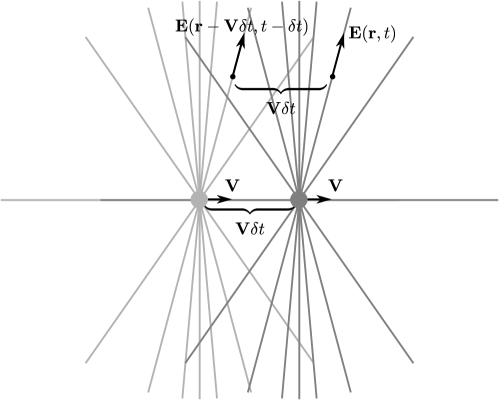
Figure 3: The stationary field of a uniformly moving point charge is in collective motion together with the point charge

$$\mathbf{E}(\mathbf{r},t) = \mathbf{E}(\mathbf{r}-\mathbf{V}\delta t,t-\delta t)$$ (28)

$$\mathbf{B}(\mathbf{r},t) = \mathbf{B}(\mathbf{r}-\mathbf{V}\delta t,t-\delta t)$$ (29)

Notice that requirement (M) says nothing about whether and how the fact that the system as a whole is at rest or in motion with some velocity is reflected in the solutions $F\in\mathcal{E}$. It does not even require that this fact can be expressed in terms of $\xi_{1},\xi_{2},\ldots\xi_{n}$. It only requires that each $F\in\mathcal{E}$ belong to a physical situation in which it is meaningful to say—perhaps in terms of quantities different from $\xi_{1},\xi_{2},\ldots\xi_{n}$—that the system is at rest or in motion relative to a reference frame. How a concrete physical situation can be characterized as such in which the system is at rest or in motion is a separate problem, which can be discussed in the particular contexts.

The second thing to be said about $M_{\mathbf{V}}(F)$ is that it is a notion determined by the concrete physical context; but it is not equal to the “Lorentz boosted solution” $T_{\mathbf{V}}^{-1}\left(P_{\mathbf{V}}(F)\right)$ by definition —as a little reflection shows:

• In this case, (8) would read

  $$T_{\mathbf{V}}^{-1}\left(P_{\mathbf{V}}(F)\right)=T_{\mathbf{V}}^{-1}\left(P_{\mathbf{V}}(F)\right)$$ (30)

  That is, the RP would become a tautology; a statement which is always true, independently of any contingent fact of nature; independently of the actual behavior of moving physical objects; and independently of the actual empirical meanings of physical quantities $\xi^{\prime}_{1},\xi^{\prime}_{2},\ldots\xi^{\prime}_{n}$. But, the RP is supposed to be a fundamental law of nature. Note that a tautology is entirely different from a fundamental principle, even if the principle is used as a fundamental hypothesis or fundamental premise of a theory, from which one derives further physical statements. For, a fundamental premise, as expressing a contingent fact of nature, is potentially falsifiable by testing its consequences; a tautology is not.

• Even if accepted, $M_{\mathbf{V}}(F)\overset{{}^{def}}{=}T_{\mathbf{V}}^{-1}\left(P_{\mathbf{V}}(F)\right)$ can provide physical meaning to $M_{\mathbf{V}}(F)$ only if we know the meanings of $T_{\mathbf{V}}$ and $P_{\mathbf{V}}$, that is, if we know the empirical meanings of the quantities denoted by $\xi^{\prime}_{1},\xi^{\prime}_{2},\ldots\xi^{\prime}_{n}$. But, the physical meaning of $\xi^{\prime}_{1},\xi^{\prime}_{2},\ldots\xi^{\prime}_{n}$ are obtained from the operational definitions: they are the quantities obtained by “the same measurements with the same equipments when they are, as a whole, co-moving with $K^{\prime}$ with velocity $\mathbf{V}$ relative to $K$”. Symbolically, we need, priory, the concepts of $M_{\mathbf{V}}(\xi_{i}\mbox{-}equipment\,at\,rest)$. And this is a conceptual circularity: in order to have the concept of what it is to be an $M_{\mathbf{V}}(brick\,at\,rest)$ the (size)’ of which we would like to ascertain, we need to have the concept of what it is to be an $M_{\mathbf{V}}(measuring\,rod\,at\,rest)$—which is exactly the same conceptual problem.

• One might claim that we do not need to specify the concepts of $M_{\mathbf{V}}(\xi_{i}\mbox{-}equipment\,at\,rest)$ in order to know the values of quantities $\xi^{\prime}_{1},\xi^{\prime}_{2},\ldots\xi^{\prime}_{n}$ we obtain by the measurements with the moving equipments, given that we can know the transformation rule $T_{\mathbf{V}}$ independently of knowing the operational definitions of $\xi^{\prime}_{1},\xi^{\prime}_{2},\ldots\xi^{\prime}_{n}$. Typically, $T_{\mathbf{V}}$ is thought to be derived from the assumption that the RP (8) holds. If however $M_{\mathbf{V}}$ is, by definition, equal to $T_{\mathbf{V}}^{-1}\circ P_{\mathbf{V}}$, then in place of (8) we have the tautology (30), which does not determine $T_{\mathbf{V}}$.

• Therefore, unsurprisingly, it is not the RP from which the transformation rules are routinely deduced, but the covariance (14). As we have seen, however, covariance is, in general, neither sufficient nor necessary for the RP. Whether (8) implies (14) hinges on the physical fact whether (16) is satisfied. But, if $M_{\mathbf{V}}$ is taken to be $T_{\mathbf{V}}^{-1}\circ P_{\mathbf{V}}$ by definition, the RP becomes true—in the form of tautology (30)—but does not imply covariance $T_{\mathbf{V}}^{-1}\circ P_{\mathbf{V}}(\mathcal{E})=\mathcal{E}$.

• Even if we assume that a “transformation rule” function $\phi^{\prime}\circ T_{\mathbf{V}}\circ\phi^{-1}$ were derived from some independent premises—from the independent assumption of covariance, for example—how do we know that the $T_{\mathbf{V}}$ we obtained and the quantities of values $\phi^{\prime}\circ T_{\mathbf{V}}\circ\phi^{-1}\left(\xi_{1},\xi_{2},\ldots\xi_{n}\right)$ are correct plugins for the RP? How could we verify that $\phi^{\prime}\circ T_{\mathbf{V}}\circ\phi^{-1}\left(\xi_{1},\xi_{2},\ldots\xi_{n}\right)$ are indeed the values measured by a moving observer applying the same operations with the same measuring equipments, etc.?—without having an independent concept of $M_{\mathbf{V}}$, at least for the measuring equipments?

• One could argue that we do not need such a verification; $\phi^{\prime}\circ T_{\mathbf{V}}\circ\phi^{-1}\left(\xi_{1},\xi_{2},\ldots\xi_{n}\right)$ can be regarded as the empirical definition of the primed quantities:

  $$\left(\xi^{\prime}_{1},\xi^{\prime}_{2},\ldots\xi^{\prime}_{n}\right)\overset{{}^{def}}{=}\phi^{\prime}\circ T_{\mathbf{V}}\circ\phi^{-1}\left(\xi_{1},\xi_{2},\ldots\xi_{n}\right)$$ (31)

  This is of course logically possible. The operational definition of the primed quantities would say: ask the observer at rest in $K$ to measure $\xi_{1},\xi_{2},\ldots\xi_{n}$ with the measuring equipments at rest in $K$, and then perform the mathematical operation (31). In this way, however, even the transformation rules would become tautologies; they would be true, no matter how the things are in the physical world.

• Someone might claim that the identity of $M_{\mathbf{V}}$ with $T_{\mathbf{V}}^{-1}\circ P_{\mathbf{V}}$ is not a simple stipulation but rather an analytic truth which follows from the identity of the two concepts. Still, if that were the case, RP would be a statement which is true in all possible worlds; independently of any contingent fact of nature; independently of the actual behavior of moving physical objects.

• On the contrary, as we have already pointed out in Remark 2, $M_{\mathbf{V}}(F)$ and $T_{\mathbf{V}}^{-1}\left(P_{\mathbf{V}}(F)\right)$ are different concepts, referring to different features of different parts of the physical reality. Any connection between the two things must be a contingent fact of the world.

• $T_{\mathbf{V}}^{-1}\circ P_{\mathbf{V}}$ is a $2^{R}\rightarrow 2^{R}$ map which is completely determined by the physical behaviors of the measuring equipments. On the other hand, whether the elements of $\mathcal{E}\subset 2^{R}$ satisfy condition (M) and whether $T_{\mathbf{V}}^{-1}\circ P_{\mathbf{V}}(\mathcal{E})\subseteq\mathcal{E}$ depend on the actual physical properties of the object physical system.

• Let us note that in the standard textbook applications of the RP $M_{\mathbf{V}}$ is used as an independent concept, without any prior reference to the Lorentz boost $T_{\mathbf{V}}^{-1}\circ P_{\mathbf{V}}$. For example, we do not need to refer to the Lorentz transformations in order to understand the concept of ‘the stationary electromagnetic field of a uniformly moving point charge’; as we are capable to solve the electrodynamical equations for such a situation, within one single frame of reference, without even knowing of the Lorentz transformation rules. $\lrcorner$

References

• How to teach special relativity, in Speakable and unspeakable in quantum mechanics. Cambridge, Cambridge University Press.

• Zur Elektrodynamik bewegter Körper, Annalen der Physik 17, 891. (On the Electrodynamics of Moving Bodies, in H. A. Lorentz et al., The principle of relativity: a collection of original memoirs on the special and general theory of relativity. London, Methuen and Company 1923)

• Special relativity and thermodynamics, Proc. Comb. Phil. Soc. 66, 423.

• Classical Electrodynamics (Third edition). Hoboken (NJ), John Wiley & Sons.

• On the meaning of Lorentz covariance, Foundations of Physics Letters 17, pp. 479–496.

• Relativity, Thermodynamics and Cosmology. Oxford, Clarendon Press.