Hermitian scattering behavior for the non-Hermitian scattering center

Abstract

We study the scattering problem for the non-Hermitian scattering center, which consists of two Hermitian clusters with anti-Hermitian couplings between them. Counterintuitively, it is shown that it acts as a Hermitian scattering center, satisfying $\left|r\right|^{2}+\left|t\right|^{2}=1,$ i.e., the Dirac probability current is conserved, when one of two clusters is embedded in the waveguides. This conclusion can be applied to an arbitrary parity-symmetric real Hermitian graph with additional $\mathcal{PT}$-symmetric potentials, which is more feasible in experiment. Exactly solvable model is presented to illustrate the theory. Bethe ansatz solution indicates that the transmission spectrum of such a cluster displays peculiar feature arising from the non-Hermiticity of the scattering center.

I Introduction

A non-Hermitian Hamiltonian is usually endowed with the physical meaning when it possesses entirely real quantum mechanical energy spectrum and the complex extension of the conventional quantum mechanics, a parity-time ($\mathcal{PT}$) symmetric quantum theory, has been well developed Bender 98 ; Bender 99 ; Dorey 01 ; Bender 02 ; A.M43 ; A.M ; A.M36 ; Jones since the seminal discovery by Bender Bender 98 . Such a theory gives the pseudo-Hermitian Hamiltonian a physical meaning via its corresponding Hermitian counterparts A.M38 ; A.M391 ; A.M392 , which has an identical spectrum. The metric-operator theory outlined in Ref. A.M provides a mapping of such a pseudo-Hermitian Hamiltonian to an equivalent Hermitian Hamiltonian. Thus, most of the studies focused on the quasi-Hermitian system, or unbroken $\mathcal{PT}$-symmetric region Joglekar82 ; Joglekar83 . However, the obtained equivalent Hermitian Hamiltonian is usually quite complicated A.M ; JLPT , involving long-range or nonlocal interactions, which is hardly realized in practice.

Experimentally, the $\mathcal{PT}$ symmetry is of great relevance to the technological applications based on the fact that the imaginary potential could be realized by complex index in optics Bendix ; Keya ; YDChong ; LonghiLaser . Furthermore, the $\mathcal{PT}$ optical potentials can be realized through a judicious inclusion of index guiding and gain/loss regions. Such non-Hermitian systems are not isolated but usually embedded in the large Hermitian waveguides. Pure imaginary potential as a scattering center breaks the conservation of the flow of probability JLCTP . Thus, it is interesting to investigate what happens when the non-Hermitian system is with balanced gain and loss as a scattering center, and much effort devoted to such a topic is based on the framework of $\eta$-metric ZAhmed ; MZnojil ; HJones ; Kivshar .

In this paper, we study the scattering problem for the non-Hermitian scattering center based on the configurations involving two arbitrary Hermitian networks coupled with anti-Hermitian interaction. It is shown that for any scattering state of such a non-Hermitian system, the Dirac probability current is always conserved at any degree of the non-Hermiticity. We apply such a rigorous result to the system with $\mathcal{PT}$-symmetric potentials, which is more feasible in experiment.

This paper is organized as follows. Section II presents the exact analytical solution of the scattering problem for the concerned non-Hermitian scattering center. Section III is the application of the rigorous result to the system with $\mathcal{PT}$-symmetric potentials. Section IV consists of an exactly solvable example to illustrate our main idea. Section V is the summary and discussion.

II Model and formalism

In general, a non-Hermitian Hamiltonian $H$ is related by a similarity transformation to an equivalent Hermitian Hamiltonian $h$. Such a connection is valid within the so called unbroken symmetric region. However, when a non-Hermitian system interacts with other Hermitian system, such a region loses its physical meaning: On the one hand, the unbroken symmetric region is shifted in the whole non-Hermitian system. On the other hand, it may act as a Hermitian system in the scattering problem without the restriction on the degree of the non-Hermiticity. In this section, we will investigate the latter situation.

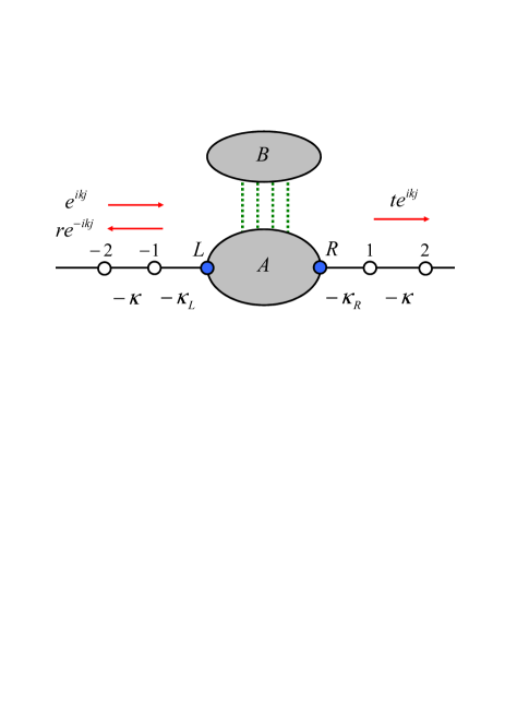
Figure 1: ((Color online) Schematic illustration of the configuration of the concerned network. It consists of two arbitrary graphs of the Hermitian tight-binding networks $A$ and $B$ (shadow) with one of them connecting to two semi-infinite chains as the waveguides at the joint sites $L$ and $R$. The non-Hermiticity of the whole scattering center $A+B$ arises from the anti-Hermitian interaction (dished lines) between them. It is shown that the non-Hermitian scattering center acts as a Hermitian one, preserving the Dirac probability current.

The Hamiltonian of the concerned scattering tight-binding network has the form

$$H=H_{L}+H_{R}+H_{C},$$ (1)

where

$$H_{L} = -\kappa\sum_{j=-1}^{-\infty}\left|j\right\rangle_{L}\left\langle j-1\right|-g_{L}\left|L\right\rangle_{L}\left\langle-1\right|+\text{H.c.},$$ (2)

$$H_{R} = -\kappa\sum_{j=1}^{+\infty}\left|j\right\rangle_{R}\left\langle j+1\right|-g_{R}\left|R\right\rangle_{R}\left\langle 1\right|+\text{H.c.},$$ (3)

represent the left ($H_{L}$) and right ($H_{R}$) waveguides with real $\kappa$ and

$$H_{C}=H_{A}+H_{B}+H_{AB}+H_{BA},$$ (4)

describes a non-Hermitian network as a scattering center. Here $\left|L\right\rangle$ and $\left|R\right\rangle$ denote the sites state on the joint sites on the network $A$, which are simply taken as $\left|L\right\rangle=\left|1\right\rangle_{A}$ and $\left|R\right\rangle=\left|N_{A}\right\rangle_{A}$ without losing the generality. The subgraphs

$$H_{A} = \sum_{i,j=1}^{N_{A}}\left(H_{A}\right)_{ij}\left|i\right\rangle_{A}\left\langle j\right|,$$ (5)

$$H_{B} = \sum_{i,j=1}^{N_{B}}\left(H_{B}\right)_{ij}\left|i\right\rangle_{B}\left\langle j\right|,$$ (6)

are arbitrary Hermitian networks, i.e., $H_{A}^{{\dagger}}=H_{A}$, and $H_{B}^{{\dagger}}=H_{B}$, while the coupling between them is anti-Hermitian, i.e., $H_{AB}^{\dagger}=-H_{BA}$.

$$H_{AB}=\sum_{i=1}^{N_{A}}\sum_{j=1}^{N_{B}}\left(H_{AB}\right)_{ij}\left|i\right\rangle_{AB}\left\langle j\right|,$$ (7)

then the scattering center with respect to the basis $\left\{\left|i\right\rangle_{A},\left|i\right\rangle_{B}\right\}$ is in the form of

$$H_{C}=\left(\begin{array}[]{cc}H_{A}&H_{AB}\\ -H_{AB}^{{\dagger}}&H_{B}\end{array}\right).$$ (8)

The non-Hermiticity of $H_{C}$ arises from this anti-Hermitian term. The non-Hermitian Hamiltonian $H_{C}$ may have fully real spectrum or not. In the following, we will show that it always acts as a Hermitian scattering center no matter the reality of the spectrum.

For an incident plane wave with momentum $k$ incoming from the left waveguide $L$ with energy $E=-2\kappa\cos k$, the scattering wave function $\left|\psi_{k}\right\rangle$ can be obtained by the Bethe ansatz method. The wave function has the form

$$\left|\psi_{k}\right\rangle=\sum_{j=-1}^{-\infty}f_{j}\left|j\right\rangle_{L}+\sum_{j=1}^{N_{A}}\alpha_{j}\left|j\right\rangle_{A}+\sum_{j=1}^{N_{B}}\beta_{j}\left|j\right\rangle_{B}+\sum_{j=1}^{+\infty}f_{j}\left|j\right\rangle_{R},$$ (9)

where the scattering wavefunction $f_{j}$ is in form of

$$f_{j}=\left\{\begin{array}[]{c}e^{ikj}+re^{-ikj},\left(j\leqslant-1\right)\\ te^{ikj},\left(j\geqslant 1\right)\end{array}\right..$$ (10)

Here $r$, $t$ are the reflection and transmission coefficients of the incident wave, which is what we concern only in this paper. Substituting the wavefunction $\left|\psi_{k}\right\rangle$ into the Schrödinger equation

$$H\left|\psi_{k}\right\rangle=E\left|\psi_{k}\right\rangle,$$ (11)

the explicit form of the Schrödinger equations in the truncated Hilbert space spanned by the basis $\left\{\left|j,j\in\left[1,N_{A}\right]\right\rangle_{A},\left|j,j\in\left[1,N_{B}\right]\right\rangle_{B}\right\}$ can be expressed in the following matrix equation form

$$\Delta\left(\begin{array}[]{c}\alpha_{1}\\ \vdots\\ \alpha_{j}\\ \vdots\\ \alpha_{N_{A}}\\ \beta_{1}\\ \vdots\\ \beta_{j}\\ \vdots\\ \beta_{N_{B}}\end{array}\right)=\left(\begin{array}[]{c}g_{L}f_{-1}\\ 0\\ \vdots\\ 0\\ g_{R}f_{1}\\ 0\\ \vdots\\ 0\\ \vdots\\ 0\end{array}\right),$$ (12)

where $\Delta$ is an $\left(N_{A}+N_{B}\right)\times$ $\left(N_{A}+N_{B}\right)$ matrix defined by

$$\Delta=\left(\begin{array}[]{cc}H_{A}-E&H_{AB}\\ -H_{AB}^{{\dagger}}&H_{B}-E\end{array}\right),$$ (13)

From the reduced Schrödinger equation of Eq. (12), we obtain

$$\alpha_{1} = \left(\Delta^{-1}\right)_{11}g_{L}f_{-1}+\left(\Delta^{-1}\right)_{1N_{A}}g_{R}f_{1},$$ (14)

$$\alpha_{N_{A}} = \left(\Delta^{-1}\right)_{N_{A}1}g_{L}f_{-1}+\left(\Delta^{-1}\right)_{N_{A}N_{A}}g_{R}f_{1},$$

Here $\Delta^{-1}$ is the inverse of matrix $\Delta$, with the element being expressed as

$$\left(\Delta^{-1}\right)_{ij}=\frac{C_{ji}}{\det\left(\Delta\right)}=\frac{\left(-1\right)^{i+j}\det\left(M_{ji}\right)}{\det\left(\Delta\right)},$$ (15)

in term of the matrix of cofactors $C_{ij}$. Here $M_{ij}$ is the matrix obtained by deleting the $i$th row and $j$th column from the matrix $\Delta$. On the other hand, the Schrödinger equations for the sites of the waveguides connecting to the joints of the scattering center are

$$-\kappa f_{-2}-g_{L}^{\ast}\alpha_{1} = Ef_{-1},$$ (16)

$$-\kappa f_{2}-g_{R}^{\ast}\alpha_{N_{A}} = Ef_{1},$$

which lead to

$$\alpha_{1}=\frac{\kappa}{g_{L}^{\ast}}\left(1+r\right)\text{, }\alpha_{N_{A}}=\frac{\kappa}{g_{R}^{\ast}}t.$$ (17)

Then associating with Eqs. (14), we have

$$r = (-b\widetilde{b}+ac-ae^{-ik}-ce^{ik}+1)/\eta,$$ (18)

$$t = i2\widetilde{b}\sin k/\eta,$$ (19)

where

$$\eta = (b\widetilde{b}-ac)e^{i2k}+\left(a+c\right)e^{ik}-1,$$

$$a = \left(\Delta^{-1}\right)_{11}\left|g_{L}\right|^{2}/\kappa\text{, }c=\left(\Delta^{-1}\right)_{N_{A}N_{A}}\left|g_{R}\right|^{2}/\kappa,$$ (20)

$$b = \left(\Delta^{-1}\right)_{1N_{A}}g_{L}^{\ast}g_{R}/\kappa\text{, }\widetilde{b}=\left(\Delta^{-1}\right)_{N_{A}1}g_{L}g_{R}^{\ast}/\kappa.$$

One can determine the unknown coefficients $a$, $b$, $\widetilde{b}$, $c$ and $\eta$ through the matrix $\Delta$ by requiring that invertible matrix $\left(H_{A}-E\right)$ or $\left(H_{B}-E\right)$ exists.

In the Appendix, we will show that

$$\left(\Delta^{-1}\right)_{ij}=\left(\Delta^{-1}\right)_{ji}^{\ast}$$ (21)

for $i,j\in[1,N_{A}]$, or more explicitly for special cases

$$\left(\Delta^{-1}\right)_{11} = \left(\Delta^{-1}\right)_{11}^{\ast},$$ (22a)

$$\left(\Delta^{-1}\right)_{N_{A}N_{A}} = \left(\Delta^{-1}\right)_{N_{A}N_{A}}^{\ast},$$ (22b)

$$\left(\Delta^{-1}\right)_{1N_{A}} = \left(\Delta^{-1}\right)_{N_{A}1}^{\ast},$$ (22c)

which indicate that both $$a c \widetilde{b}=b^{\ast}$$ and are real, and . It is somewhat surprising that we get the conclusion from Eqs. (18), (19), (20) and (22) that

$$\left|r\right|^{2}+\left|t\right|^{2}=1,$$ (23)

which is common phenomenon in a Hermitian system but surprising in a non-Hermitian system.

III $\mathcal{PT}$-symmetric potentials

The accessible setup of non-Hermitian system in the lab is the $\mathcal{PT}$-symmetric potentials, which can be realized through a judicious inclusion of index guiding and gain/loss regions. In the following, we will apply the obtained result to the system with the $\mathcal{PT}$-symmetric potentials, in which the $\mathcal{PT}$-symmetrical axis is along the waveguides.

The geometry of the scattering center contains $N_{1}+2N_{2}$ sites and possesses the following symmetry,

$$\begin{array}[]{l}\mathcal{P}:\left|j\right\rangle_{c}\longrightarrow\left|j\right\rangle_{c},\text{ }\left(j\in\left[1,N_{1}\right]\right)\\ \mathcal{P}:\left|j\right\rangle_{c}\longrightarrow\overline{\left|j\right\rangle}_{c}=\left|N_{2}+j\right\rangle_{c},\text{ }\left(j-N_{1}\in\left[1,N_{2}\right]\right)\end{array}$$ (24)

with the joint points $L,$ $R$ $\in\left[1,N_{1}\right]$, where $\overline{\left|j\right\rangle}_{c}$ is the mirror symmetric counterpart of state $\left|j\right\rangle_{c}$. We define the Hamiltonian of the center has the form

$$H_{\mathcal{PT}}=\sum_{i,j=1,\left(i<j\right)}^{N_{1}+2N_{2}}\kappa_{ij}\left|i\right\rangle_{c}\left\langle j\right|+\text{H.c.}$$ (25)

$$+\sum_{j=1}^{N_{1}}U_{j}\left|j\right\rangle_{c}\left\langle j\right|+\sum_{j=N_{1}+1}^{N_{1}+N_{2}}(V_{j}\left|j\right\rangle_{c}\left\langle j\right|+V_{j}^{\ast}\overline{\left|j\right\rangle}_{c}\overline{\left\langle j\right|}),$$

where $\kappa_{ij}$ and $U_{j}$ are real. In the Hilbert space spanned by basis $\left\{\left|j\right\rangle_{c}\right\}$ $\left(j\in\left[1,N_{1}+2N_{2}\right]\right)$, the matrix of the Hamiltonian $H_{\mathcal{PT}}$ has the form

$$H_{\mathcal{PT}}=\left(\begin{array}[]{ccc}H_{\gamma}&H_{\gamma\alpha}&H_{\gamma\alpha}\\ H_{\gamma\alpha}^{\dagger}&H_{\alpha}+H_{\delta}&H_{\alpha\beta}\\ H_{\gamma\alpha}^{\dagger}&H_{\alpha\beta}&H_{\alpha}-H_{\delta}\end{array}\right),$$ (26)

where

$$\left(H_{\delta}\right)_{ij}=\delta_{ij}(V_{j}-V_{j}^{\ast})/2=i\text{Im}\left(V_{j}\right)\delta_{ij}$$ (27)

and $H_{\gamma}$ ($H_{\alpha}$) is an $N_{1}$ ($N_{2}$) dimension square matrix. The matrices $H_{\gamma}$, $H_{\alpha}$, and $H_{\alpha\beta}$ are all real Hermitian while $H_{\gamma\alpha}$ is real. We can see that Hamiltonian $H_{\mathcal{PT}}$ describes an arbitrary real Hermitian graph with parity-symmetry as defined in Eq. (24) combining with the on-site $\mathcal{PT}$-symmetric potentials $H_{\delta}$. Thus $H_{\mathcal{PT}}$ satisfies $\left[\mathcal{PT}\text{, }H_{\mathcal{PT}}\right]=0$.

Introducing the linear transformation

$$\left|j\right\rangle_{A} = \left\{\begin{array}[]{cc}\left|j\right\rangle_{c},&\left(j\in\left[1,N_{1}\right]\right)\\ (\left|j\right\rangle_{c}+\overline{\left|j\right\rangle}_{c})/\sqrt{2},&\left(j-N_{1}\in\left[1,N_{2}\right]\right)\end{array}\right.$$ (28c)

$$\left|j\right\rangle_{B} = (\left|j\right\rangle_{c}-\overline{\left|j\right\rangle}_{c})/\sqrt{2},\text{ }\left(j-N_{1}\in\left[1,N_{2}\right]\right)$$ (28d)

one can rewrite the matrix of Eq. (26) in the basis $$\left\{\left|j\text{, }j\in\left[1,N_{1}+N_{2}\right]\right\rangle_{A}\right. \left.\left|j\text{, }j\in\left[N_{1}+1,N_{1}+N_{2}\right]\right\rangle_{B}\right\}$$, as the form

$$H_{\mathcal{PT}}=\left(\begin{array}[]{ccc}H_{\gamma}&\sqrt{2}H_{\gamma\alpha}&0\\ \sqrt{2}H_{\gamma\alpha}^{\dagger}&H_{\alpha}+H_{\alpha\beta}&H_{\delta}\\ 0&H_{\delta}&H_{\alpha}-H_{\alpha\beta}\end{array}\right)$$ (29)

Obviously, it is the special case of Eq. (8), where

$$H_{A} = \left(\begin{array}[]{cc}H_{\gamma}&\sqrt{2}H_{\gamma\alpha}\\ \sqrt{2}H_{\gamma\alpha}^{\dagger}&H_{\alpha}+H_{\alpha\beta}\end{array}\right),$$ (32)

$$H_{B} = H_{\alpha}-H_{\alpha\beta},$$ (33)

$$H_{AB} = \left(\begin{array}[]{c}0\\ H_{\delta}\end{array}\right),H_{BA}=\left(\begin{array}[]{cc}0&H_{\delta}\end{array}\right),$$ (37)

or equivalently in the explicit form as

$$\left(H_{A}\right)_{mn}\left.=\right._{A}\left\langle m\right|H_{\mathcal{PT}}\left|n\right\rangle_{A} = \left(H_{A}\right)_{nm}^{\ast},$$ (38)

$$\left(H_{B}\right)_{mn}\left.=\right._{B}\left\langle m\right|H_{\mathcal{PT}}\left|n\right\rangle_{B} = \left(H_{B}\right)_{nm}^{\ast},$$ (39)

$$\left(H_{AB}\right)_{mn}\left.=\right._{A}\left\langle m\right|H_{\mathcal{PT}}\left|n\right\rangle_{B} = i\text{Im}\left(V_{m}\right)\delta_{m-N_{1},n},$$ (40)

$$\left(H_{BA}\right)_{mn}\left.=\right._{B}\left\langle m\right|H_{\mathcal{PT}}\left|n\right\rangle_{A} = i\text{Im}\left(V_{n}\right)\delta_{m,n-N_{1}}.$$ (41)

Therefore, the cluster $H_{\mathcal{PT}}$ acts as a Hermitian scattering center. This result is independent of the magnitudes of the hopping integrals and the potentials, also the reality of the spectrum of $H_{\mathcal{PT}}$.

IV Illustration

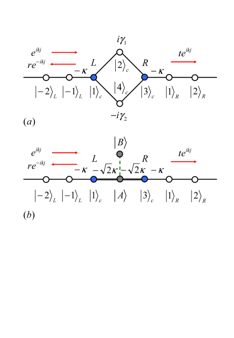
Figure 2: (Color online) Schematic illustration for the exemplified system. (a) $4$-site non-Hermitian scattering center configuration, which consists of two on-site imaginary potentials $i\gamma_{1}$ and $-i\gamma_{2}$ connecting to two semi-infinite chains as the waveguides at the joint sites $\left|1\right\rangle_{c}$ and $\left|3\right\rangle_{c}$, with the hopping strength $-\kappa$. (b) The equivalent Hamiltonian of $H_{C}$ [Eq. (IV)], which is obtained under the linear transformation of Eq. (52). The hopping strengths between the site $\left|A\right\rangle$ and $\left|1\right\rangle_{c}$, $\left|3\right\rangle_{c}$ are both $-\sqrt{2}\kappa$. The dashed (green) line represents the effective hopping between sites $\left|A\right\rangle$ and $\left|B\right\rangle\$which is pure imaginary $i\left(\gamma_{1}+\gamma_{2}\right)/2$, with both potentials on $\left|A\right\rangle$ and $\left|B\right\rangle$ being $i\left(\gamma_{1}-\gamma_{2}\right)/2$. In the case of $\gamma_{1}=\gamma_{2}$, it is shown that the non-Hermitian scattering center acts as a Hermitian one, preserving the Dirac probability current.

We consider a simple $4$-site non-Hermitian scattering center which is illustrated schematically in Fig. 2(a). The Hamiltonian of the whole system of Eq. (1) can be written as

$$H_{L} = -\kappa\sum_{j=-1}^{-\infty}\left|j\right\rangle_{L}\left\langle j-1\right|-\kappa\left|-1\right\rangle_{Lc}\left\langle 1\right|+\text{H.c.},$$ (42)

$$H_{R} = -\kappa\sum_{j=1}^{+\infty}\left|j\right\rangle_{R}\left\langle j+1\right|-\kappa\left|1\right\rangle_{Rc}\left\langle 3\right|+\text{H.c.},$$ (43)

where the joints of the scattering center are $L=1$, $R=3$ and

$$H_{C} = -\kappa\left(\left|1\right\rangle_{c}\left\langle 2\right|+\left|2\right\rangle_{c}\left\langle 3\right|+\left|3\right\rangle_{c}\left\langle 4\right|+\left|4\right\rangle_{c}\left\langle 1\right|+\text{H.c.}\right)$$ (44)

$$+i\gamma_{1}\left|2\right\rangle_{c}\left\langle 2\right|-i\gamma_{2}\left|4\right\rangle_{c}\left\langle 4\right|.$$

Note that here we consider a non-$\mathcal{PT}$-symmetric model without losing the generality. The Bethe ansatz wavefunction has the form

$$\left|\phi_{k}\right\rangle=\sum_{j=-1}^{-\infty}f_{j}\left|j\right\rangle_{L}+\sum_{j=1}^{4}h_{j}\left|j\right\rangle_{c}+\sum_{j=1}^{+\infty}f_{j}\left|j\right\rangle_{R},$$ (45)

where $f_{j}$ is in form of Eq. (10). Taking $\kappa=1$, the explicit form of Schrödinger equations are

$$-f_{-1}-h_{2}-h_{4} = Eh_{1},$$

$$-f_{1}-h_{2}-h_{4} = Eh_{3},$$

$$-h_{1}-h_{3} = \left(E-i\gamma_{1}\right)h_{2},$$ (46)

$$-h_{1}-h_{3} = \left(E+i\gamma_{2}\right)h_{4},$$

$$E = -2\cos k.$$

the continuity of the wavefunctions demands

$$h_{1}=1+r,h_{3}=t,$$ (47)

The corresponding transmission and reflection coefficients have the form

$$r = \frac{\zeta\cos k-1}{e^{-ik}-\zeta}e^{ik},$$ (48)

$$t = -\frac{i\zeta\sin k}{e^{-ik}-\zeta}e^{ik},$$ (49)

where

$$\zeta=\frac{1}{\cos k+i\gamma_{1}/2}+\frac{1}{\cos k-i\gamma_{2}/2}.$$ (50)

Straightforward algebra shows that

$$\left|r\right|^{2}+\left|t\right|^{2}=1-\frac{2\text{Im}\left(\zeta\right)\sin k}{1+\left|\zeta\right|^{2}-2\text{Re}\left(\zeta\right)\cos k+2\text{Im}\left(\zeta\right)\sin k},$$ (51)

which indicates the current is conserved when $\zeta$ is real, i.e., $\gamma_{1}=\gamma_{2}$.

Alternatively, taking the linear transformation

$$\left|A\right\rangle = \left(\left|2\right\rangle_{c}+\left|4\right\rangle_{c}\right)/\sqrt{2},$$ (52a)

$$\left|B\right\rangle = \left(\left|2\right\rangle_{c}-\left|4\right\rangle_{c}\right)/\sqrt{2},$$ (52b)

the Hamiltonian $$H_{C}$$ can be rewritten as

$$H_{C} = -\sqrt{2}\kappa\left(\left|A\right\rangle_{c}\left\langle 1\right|+\left|A\right\rangle_{c}\left\langle 3\right|+\text{H.c.}\right)$$

$$+i\frac{\left(\gamma_{1}-\gamma_{2}\right)}{2}\left(\left|A\right\rangle\left\langle A\right|+\left|B\right\rangle\left\langle B\right|\right)$$

$$+i\frac{\left(\gamma_{1}+\gamma_{2}\right)}{2}\left(\left|A\right\rangle\left\langle B\right|+\left|B\right\rangle\left\langle A\right|\right),$$

as illustrated schematically in Fig. 2(b). It depicts a scattering configuration with single side coupling site which has been systematically studied in the Hermitian regime JLtrap . Obviously, when $\gamma_{1}=\gamma_{2}=\gamma$, it is a simple example of a real Hermitian graph with parity-symmetry combining with the on-site $\mathcal{PT}$-symmetric potentials and admits the current preserving.

Accordingly, the transmission probability (coefficient) has the form

$$T\left(k\right)=\frac{\sin^{2}\left(2k\right)}{\sin^{2}\left(2k\right)+\left(\cos^{2}\left(k\right)-\gamma^{2}/4\right)^{2}},$$ (54)

which has peculiar feature in contrast to that of Hermitian scattering center. As a comparison, we write the transmission probability for the real side coupling by substituting $\gamma$ with $i\gamma$, i.e.,

$$T^{\prime}\left(k\right)=\frac{\sin^{2}\left(2k\right)}{\sin^{2}\left(2k\right)+\left(\cos^{2}\left(k\right)+\gamma^{2}/4\right)^{2}}.$$ (55)

It can be observed that, (i) both of them have the common total reflection points, $T\left(\pi/2\right)=T^{\prime}\left(\pi/2\right)=0$; (ii) $T\left(k\right)=1$ at the resonance condition $\gamma=2\left|\cos k\right|$, while $T^{\prime}\left(k\right)$ is always less than $1$ within the whole range of $\gamma$.

V Summary and discussion

We have proposed an anti-Hermitian coupled two Hermitian graphs as the scattering center, which has been shown to act as a Hermitian graph, preserving the traditional probability. This conclusion can be applied to the non-Hermitian scattering center which consists of pairs of $\mathcal{PT}$-symmetric on-site potentials. This fact indicates the balanced gain and loss can result in the Hermiticity of the scattering center. Our results can give a good prediction for the transmission and reflection coefficients of linear waves scattered at the $\mathcal{PT}$-symmetric defects in the experiment. The recent observation of breaking of $\mathcal{PT}$ symmetry in coupled optical waveguides AGuo ; TK ; CERuter may pave the way to demonstrate the result presented in this paper.

Finally, we would like to point that our conclusion can also apply to other type of non-Hermitian scattering center. For instance, we can select $H_{\gamma}$, $H_{\alpha}$, $H_{\gamma\alpha}$ and $H_{\alpha\beta}$ being all Hermitian instead of real Hermitian in Eq. (26), and we note that $H_{\mathcal{PT}}$ is no longer $\mathcal{PT}$-symmetric if the hoppings are not all real, with $H_{\gamma}$, $H_{\alpha}$, $H_{\gamma\alpha}$ and $H_{\alpha\beta}$ being Hermitian, we could also select $H_{\mathcal{PT}}$ as

$$H_{\mathcal{PT}}=\left(\begin{array}[]{ccc}H_{\gamma}&H_{\gamma\alpha}&H_{\gamma\alpha}\\ H_{\gamma\alpha}^{\dagger}&H_{\alpha}+H_{\delta}&H_{\alpha\beta}\\ H_{\gamma\alpha}^{\dagger}&H_{\alpha\beta}^{\ast}&H_{\alpha}-H_{\delta}\end{array}\right).$$ (56)

which is also in form of Eq. (8) after the transformation of Eq. (28) and exhibits the Hermitian behavior.

VI Appendix

In this Appendix, we will prove the relation of Eq. (21). For an incident plane wave with real energy $E$, we obtain from Eq. (13) and $H_{A}=H_{A}^{\dagger}$, $H_{B}=H_{B}^{\dagger}$ that

$$\Delta^{\dagger}=\left(\begin{array}[]{cc}H_{A}-E&-H_{AB}\\ H_{AB}^{{\dagger}}&H_{B}-E\end{array}\right)$$ (57)

Considering the block matrix $\Delta$ and $\Delta^{\dagger}$, when $\left(H_{B}-E\right)$ is invertible, employing the Leibniz formula, we have

$$\det\left(\Delta\right) = \det\left(H_{B}-E\right)\det[\left(H_{A}-E\right)$$

$$-H_{AB}\left(H_{B}-E\right)^{-1}\left(-H_{AB}\right)^{{\dagger}}],$$

and also

$$\det\left(\Delta^{\dagger}\right) = \det\left(H_{B}-E\right)\det[\left(H_{A}-E\right)$$

$$-\left(-H_{AB}\right)\left(H_{B}-E\right)^{-1}H_{AB}^{{\dagger}}].$$

Then we have

$$\det\left(\Delta\right)=\det\left(\Delta^{\dagger}\right)=\left[\det\left(\Delta^{T}\right)\right]^{\ast}=\left[\det\left(\Delta\right)\right]^{\ast},$$ (60)

i.e., $\det\left(\Delta\right)$ is real. Such feature arises from the special structure of the matrix $\Delta$ in the form

$$\left(\begin{array}[]{cc}\mathcal{A}&\mathcal{C}\\ -\mathcal{C}^{{\dagger}}&\mathcal{B}\end{array}\right),$$ (61)

with $\mathcal{A}$ and $\mathcal{B}$ being Hermitian matrices.

Matrix $M_{ij}$ ($i,j\in\left[1,N_{A}\right]$) is obtained from $\Delta$ by eliminating its $i$th row and $j$th column, which has the form

$$\left(\begin{array}[]{cc}\mathcal{A}^{\prime}&\mathcal{C}^{\prime}\\ \mathcal{D}^{\prime}&\mathcal{B}\end{array}\right),$$ (62)

and accordingly $\left(M_{ji}\right)^{{\dagger}}$ has the form

$$\left(\begin{array}[]{cc}\mathcal{A}^{\prime}&-\mathcal{C}^{\prime}\\ -\mathcal{D}^{\prime}&\mathcal{B}\end{array}\right).$$ (63)

Here, $\mathcal{A}^{\prime}$ is the matrix by eliminating the $i$th row and $j$th column from $\mathcal{A}$, while $\mathcal{C}^{\prime}$ ($\mathcal{D}^{\prime}$) is the matrix by eliminating the $i$th row ($j$th column) from $\mathcal{C}$ ($\mathcal{D}$). By similar procedure in obtaining Eqs. (VI) and (VI), we have

$$\det\left(M_{ij}\right)=\det[\left(M_{ji}\right)^{{\dagger}}],$$ (64)

and then

$$\det\left(M_{ij}\right)=\left[\det\left(M_{ji}\right)\right]^{\ast}.$$ (65)

Together with Eq. (15), we have $\left(\Delta^{-1}\right)_{ij}=\left(\Delta^{-1}\right)_{ji}^{\ast}$, and yield Eq. (22).

References

• (1) C. M. Bender, and S. Boettcher, Phys. Rev. Lett. 80, 5243 (1998).
• (2) C. M. Bender, S. Boettcher, and P. N. Meisinger, J. Math. Phys. 40, 2201 (1999).
• (3) P. Dorey, C. Dunning, and R. Tateo, J. Phys. A: Math. Gen. 34, L391 (2001); P. Dorey, C. Dunning, and R. Tateo, J. Phys. A: Math. Gen. 34, 5679 (2001).
• (4) C. M. Bender, D. C. Brody, and H. F. Jones, Phys. Rev. Lett. 89, 270401 (2002).
• (5) A. Mostafazadeh, J. Math. Phys. 43, 3944 (2002).
• (6) A. Mostafazadeh and A. Batal, J. Phys. A: Math. Gen. 37, 11645 (2004).
• (7) A. Mostafazadeh, J. Phys. A: Math. Gen. 36, 7081 (2003).
• (8) H. F. Jones, J. Phys. A: Math. Gen. 38, 1741 (2005).
• (9) A. Mostafazadeh, J. Phys. A: Math. Gen. 38, 6557 (2005).
• (10) A. Mostafazadeh, J. Phys. A: Math. Gen. 39, 10171 (2006).
• (11) A. Mostafazadeh, J. Phys. A: Math. Gen. 39, 13495 (2006).
• (12) Y. N. Joglekar, D. Scott, M. Babbey, and A. Saxena, Phys. Rev. A 82, 030103(R) (2010).
• (13) D. D. Scott and Y. N. Joglekar, Phys. Rev. A 83, 050102(R) (2011).
• (14) L. Jin and Z. Song, Phys. Rev. A 80, 052107 (2009).
• (15) O. Bendix, R. Fleischmann, T. Kottos and B. Shapiro, Phys. Rev. Lett. 103, 030402 (2009).
• (16) K. Zhou, Z. Guo, J. Wang and S. Liu Opt. Lett. 35, 2928 (2010).
• (17) Y. D. Chong, Li Ge, Hui Cao and A. D. Stone, Phys. Rev. Lett. 105, 053901 (2010).
• (18) S. Longhi, Phys. Rev. A 82, 031801(R) (2010); Phys. Rev. Lett. 105, 013903 (2010).
• (19) L. Jin and Z. Song, Phys. Rev. A 81, 032109 (2010); Commun. Theor. Phys. 54, 73 (2010).
• (20) Z. Ahmed, Phys. Lett. A 324, 152 (2004).
• (21) M. Znojil, J. Phys. A: Math. Gen. 39, 13325 (2006); Phys. Rev. D 78, 025026 (2008); Phys. Rev. D 80, 045009 (2009).
• (22) H. F. Jones, Phys. Rev. D 76, 125003 (2007); Phys. Rev. D 78, 065032 (2008).
• (23) S. V. Dmitriev, S. V. Suchkov, A. A. Sukhorukov, and Y. S. Kivshar Phys. Rev. A 84, 013833 (2011).
• (24) L. Jin and Z. Song, Phys. Rev. A 81, 022107 (2010).
• (25) A. Guo, G. J. Salamo, D. Duchesne, R.Morandotti, M. Volatier-Ravat, V. Aimez, G. A. Siviloglou, and D. N. Christodoulides, Phys. Rev. Lett. 103, 093902 (2009).
• (26) T. Kottos, Nature Phys. 6, 166 (2010).
• (27) C. E. Rüter, K. G. Makris, R. El-Ganainy, D. N. Christodoulides, M. Segev, and D. Kip, Nature Phys. 6, 192 (2010).