The Polarization Properties of Inverse Compton Emission and Implications for Blazar Observations with the GEMS X-Ray Polarimeter

Abstract

NASA’s Small Explorer Mission GEMS (Gravity and Extreme Magnetism SMEX), scheduled for launch in 2014, will have the sensitivity to detect and measure the linear polarization properties of the 0.5 keV and 2-10 keV X-ray emission of a considerable number of galactic and extragalactic sources. The prospect of sensitive X-ray polarimetry justifies a closer look at the polarization properties of the basic emission mechanisms. In this paper, we present analytical and numerical calculations of the linear polarization properties of inverse Compton scattered radiation. We describe a generally applicable formalism that can be used to numerically compute the polarization properties in the Thomson and Klein-Nishina regimes. We use the code to perform for the first time a detailed comparison of numerical results and the earlier analytical results derived by Bonometto et al. (1970) for scatterings in the Thomson regime. Furthermore, we use the numerical formalism to scrutinize the polarization properties of synchrotron self-Compton emission, and of inverse Compton radiation emitted in the Klein-Nishina regime. We conclude with a discussion of the scientific potential of future GEMS observations of blazars. The GEMS mission will be able to confirm the synchrotron origin of the low-energy emission component from high frequency peaked BL Lac objects. Furthermore, the observations have the potential to decide between a synchrotron self-Compton and external-Compton origin of the high-energy emission component from flat spectrum radio quasars and low frequency peaked BL Lac objects.

1 Introduction

Although the scientific potential of X-ray polarimetry observations has long been appreciated (e.g. Rees, 1975; Lightman & Shapiro, 1975, 1976; Meszaros et al., 1988), only a single dedicated X-ray polarimeter mission has been flown so far: the OSO-8 mission launched in 1975 (Novick et al., 1977). The mission was able to detect polarization degrees of a few percent for X-ray bright sources with Crab-like fluxes. This sensitivity was sufficient to detect the polarization of one cosmic source. The observations of the Crab nebula revealed evidence for linear polarization at 2.6 keV and 5.2 keV at a level of $\sim$20% (Weisskopf et al., 1978). More recently, the INTEGRAL satellite was used to study the polarization of the Crab Nebula and Cyg X-1 (Dean et al., 2008; Forot et al., 2008; Laurent et al., 2011). Even though the observations suggest polarization degrees of $\stackrel{{\scriptstyle>}}{{\scriptstyle\sim}}$40% in the hard X-ray/$\gamma$-ray regime, the systematic uncertainties on these results are large. NASA plans to launch the Small Explorer Mission GEMS (Gravity and Extreme Magnetism SMEX) in 2014, a dedicated mission for X-ray polarimetry in the 2-10 keV energy range, with the sensitivity to detect polarization degrees down to $\sim 1$% even for weak sources with a flux of a few mCrab (Black et al., 2010). A student experiment will extend the polarimetric measurement capabilities into sub-keV energy range (Kaaret et al., 2009). GEMS will be able to measure the polarization properties of dozens of galactic and extragalactic sources and to establish X-ray polarimetry as an observational discipline. The main science drivers of GEMS are the measurement of the orientation and inclination of the inner accretion disks and the masses and spins of Binary Black Hole systems (BBHs), the detection of plasma physics effects in neutron star magnetospheres, the study of the locale and properties of the particle acceleration regions in pulsars and pulsar wind nebulae, and the study of the coronae and jets of Active Galactic Nuclei (AGNs) (see Lei, Dean, Hills et al., 1997; Weisskopf et al., 2006; Bellazini et al., 2010; Krawczynski, 2011).
The upcoming launch of the GEMS mission motivates a close look at the polarization properties of the most common X-ray emission processes. Whereas the polarization properties of synchrotron emission, Bremsstrahlungs emission, and Thomson scattered emission are well studied (e.g. Ginzburg & Syrovatskii, 1965; Dolan, 1967; Laing, 1980; Bjornsson & Blumenthal, 1982; Bjornsson, 1985; Rybicki & Lightman, 1986; Begelman, 1993; Ruszkowski & Begelman, 2002, and references therein), a similar in-depth understanding of the polarization properties of inverse Compton emission is still lacking. In the following, “Inverse Compton” denotes the emission from a single up-scattering of low-frequency target photons by relativistic electrons. Prime examples of inverse Compton emission include the high-energy component of AGNs and possibly $\gamma$-ray emission from Gamma-Ray Bursts. This paper focuses on the polarization of inverse Compton emission and the application of the results to AGN jets. We will not discuss the polarization of “Comptonized” emission (e. g. from AGN coronae), which underwent many Compton and inverse Compton scatterings before leaving the source. Inverse Compton scatterings tend to reduce the polarization degree of emission; multiple Compton scatterings do so even more.

The polarization of inverse Compton emission usually arises from averaging the results from elemental scattering processes over a range of electron energies and propagation directions. Highly relativistic electrons with Lorentz factors $\gamma\gg 1$ scatter photons into a narrow cone centered on their propagation direction with an opening angle of $2/\gamma$. The inverse Compton emission from a relativistic electron plasma thus comes from electrons with velocities aligned to within $\sim\gamma^{-1}$ with the line of sight. In this paper, we discuss the case that the angular distribution of the electrons contributing to the observed emission does not deviate appreciably from isotropy in the rest frame of the emitting plasma, called the plasma frame (PF) in the following. For large $\gamma$-values most electron populations will satisfy this criterium.

The paper of Bonometto, Cazzola, & Saggion (1970) (called BCS in the following) reports on the polarization of the inverse Compton emission on the basis of a quantum mechanical scattering calculation. The study makes a series of approximations and is limited to highly relativistic electrons ($\gamma\gg 1$) and scatterings in the Thomson regime $\gamma(\hbar\omega/m_{\rm e}c^{2})\ll 1$ where $\omega$ denotes the frequency of the target photons. The paper presents equations to compute the polarization degree of the inverse Compton emission from isotropic electrons with arbitrary energy spectra scattering monoenergetic unidirectional photons. The authors note that the results imply a vanishing polarization degree for the inverse Compton emission from unpolarized target photon beams. In a follow-up paper, Bonometto & Saggion (1973) (referred to as BS in the following) describe a study of the polarization of the synchrotron self-Compton (SSC) emission from electrons in a magnetic field inverse Compton scattering their synchrotron emission. The calculation involves the numerical integration of the BCS equations. Nagirner & Poutanen (1993) confirm the analytical results of BCS and cast the results into the form of a scattering matrix which operates on the Stokes vector of the target beam. The authors evaluate the scattering matrix for power law and Maxwellian electron distributions, and Poutanen (1994) uses these results to discuss some aspects of the polarization of SSC emission.

The shortcoming of all the analytical calculations is that it is not clear at which Lorentz factors the results start to be valid, and how accurate the predicted polarization degrees are in any specific case. Various authors have thus developed codes to numerically evaluate the polarization degrees. Begelman & Sikora (1987) describe a formalism to numerically compute the polarization of inverse Compton scattered unpolarized target beams in the Thomson regime. They use this formalism to study the polarization of electron beams (“AGN jets”) with finite opening angles and with different internal structures (e. g. filled and hollow cones). Most of their discussion focuses on situations in which the observer is either not looking directly into a modestly relativistic electron beam, or that the intensity of the electron beam varies strongly over angular scales of $\gamma^{-1}$.

Celotti & Matt (1994) (called CM in the following) extend the formalism of Begelman & Sikora (1987) to treat partially polarized beams and present numerical results concerning the polarization of SSC emission from power law electron populations. They find that SSC emission is highly polarized - although somewhat less than the synchrotron emission. The polarization direction of the SSC emission aligns with that of the synchrotron emission, i. e. the electric field vectors of the synchrotron and SSC emission are perpendicular to the projection of the magnetic field lines in the PF onto the plane of the sky. While the results depend somewhat on the electron Lorentz factors in the mildly relativistic regime, they are largely independent of $\gamma$ for $\gamma\raisebox{-2.15277pt}{\mbox{$\stackrel{{\scriptstyle>}}{{\scriptstyle\sim}}$}}10$. Their calculations also show that unpolarized synchrotron photons give rise to SSC emission with vanishing or very small ($<5\%$) polarization degrees for all but very low Lorentz factors. Although the results of CM deviate by $\sim 15\%$ from those of BS, the authors do not investigate the origin of this discrepancy.

More recently, McNamara et al. (2009) (see McNamara et al., 2008, for additional information on the numerical algorithm) report on simulations of the emission from AGNs for specific geometries and for various unpolarized (accretion disk emission, cosmic microwave background (CMB)) and polarized (SSC emission) target photon fields. Among other cases, they compute the polarization of inverse Compton scattered unpolarized CMB emission. They report a polarization of $\sim$20% in contradiction to the predictions of BCS of a vanishingly small net-polarization.

In this paper, we re-evaluate the polarization properties of inverse Compton and SSC emission based on both analytical and numerical calculations. We describe for the first time detailed comparisons of analytical and numerical results. The comparisons show in which regimes the analytical approximations can be used. Our discussion focuses on establishing the general properties of inverse Compton scattered emission. In this spirit, we discuss SSC emission as a special case of inverse Compton emission. Although we show some results for mildly relativistic electrons ($\gamma$-values of 2 and 5), we focus the discussion on the regime $\gamma\raisebox{-2.15277pt}{\mbox{$\stackrel{{\scriptstyle>}}{{\scriptstyle\sim}}$}}10$, where the polarization degree and direction have simple dependencies on the relative orientation of the electron momentum, target photon momentum, and target photon polarization vectors. We use the numerical simulations to investigate the discrepancies between the analytical and semi-analytical results of BCS and BS on the one hand, and the numerical results of CM and McNamara et al. (2009) on the other hand. Furthermore, we present for the first time calculations of the polarization degree of inverse Compton radiation emitted by isotropic electrons in the Klein-Nishina regime.

In Section 2 we describe a generally applicable formalism that can be used to simulate inverse Compton emission from arbitrary electron and target photon distributions. The formalism can be used for arbitrary electron Lorentz factors and for scatterings in the Thomson and in the Klein-Nishina regimes, and permits the simulation of SSC processes. In Sections 3.1 and 3.2 we review the results from BCS and BS for the Thomson regime, and use them to derive analytical expressions for the intensity and polarization of the inverse Compton emission from monoenergetic electrons incident on monoenergetic unidirectional target photons. In Section 3.3 we perform detailed comparisons of the analytical and numerical results. The discussion covers the emission from monoenergetic electron and photon beams, from isotropic power law electrons scattering monoenergetic unidirectional photons, and from isotropic power law electrons scattering power law synchrotron emission. We scrutinize the polarization properties of inverse Compton scattered unpolarized CMB photons in Section 3.4, and study the polarization properties of inverse Compton radiation emitted in the Klein-Nishina regime in Section 3.5. Section 4 ends the paper with a summary and a discussion of the scientific potential of AGN observations with GEMS.

2 Monte Carlo simulations of inverse Compton processes in the Thomson and Klein-Nishina regimes

2.1 General approach, Stokes vectors, and useful functions

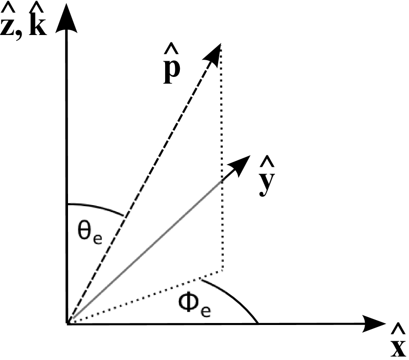
Figure 1: Sketch of the simulation set-up in the plasma frame. An unidirectional beam of electrons propagating along the direction ${\bf\hat{p}}$ with polar coordinates $(\theta_{\rm e},\phi_{\rm e})$ scatters an unidirectional photon beam propagating along the ${\bf\hat{k}}={\bf\hat{z}}$.

The numerical calculation uses a Monte Carlo approach that avoids some of the problems of earlier calculations based on integration over the entire phase space. Celotti & Matt (1994) use the latter approach and describe its difficulties: “For high values of the Lorentz factor $\gamma$, the functions in the integrals are strongly peaked in the electron direction. This requires the adoption of a carefully sampled angular grid over which to perform the angular grid…”. In contrast, the Monte Carlo approach generates events with a relative frequency matching their natural occurrence and thus makes good use of the computational resources, even in the extremely relativistic regime. The simulation of inverse Compton processes resembles in some aspects the simulation of Compton scatterings (e.g. Matt et al., 1996; Depaola, 2003) with the added complication of a Dopper boost from the PF to the electron rest frame (EF) and back. The calculation begins and ends in the PF. We use a right-handed set of unit vectors $C\equiv\{{\bf\hat{x},\,\hat{y},\,\hat{z}}\}$ to define a reference coordinate system in the PF. Initially, we consider monoenergetic unidirectional electrons with an energy-momentum four-vector $p=(\gamma m_{\rm e}c,{\bf p})$ scattering a monoenergetic unidirectional beam of photons with the four-vector $k=(\omega/c,{\bf k})$ with ${\bf\hat{k}}={\bf\hat{z}}$ (see Figure 1).
We use unit-less Stokes vectors ${\bf s}=(i,q,u)$ to track information about the statistical weight ($i$) and the linear polarization properties (via $q/i$ and $u/i$) of the simulated photons. Conceptually, we adopt the quantum mechanical treatment of the Stokes parameters described by McMaster (1961). Accordingly, the Stokes parameters are expectation values of measurement results on statistical ensembles of incoherent photons. The additive property of the Stokes parameters makes them the tool of choice for the numerical treatment, as the results from many scattering processes can be combined by adding the Stokes vectors.
In the following, we will define Stokes vectors ${\bf s}_{\rm a}$ relative to various coordinate systems $C_{\rm a}\,\equiv\{{\bf\hat{x}_{\rm a}},{\bf\hat{y}_{\rm a}},{\bf\hat{z}}_{\rm a}\}$ with the $z$-axes always aligned with the photon propagation direction. When defining new coordinate systems below, we will only give the $y$ and $z$ unit vectors, as ${\bf\hat{x}}_{\rm a}$ can always be computed from ${\bf\hat{x}}_{\rm a}={\bf\hat{y}}_{\rm a}\times{\bf\hat{z}}_{\rm a}$. We use the convention that a Stokes vector ${\bf s}_{\rm a}=(1,1,0)$ refers to a 100% linearly polarized photon beam with the electric field vector ${\hat{\boldsymbol{\varepsilon}}}$ parallel to ${\bf\hat{q}_{+}}\,\equiv{\bf\hat{y}_{\rm a}}$. The Stokes vector ${\bf s}_{\rm a}=(1,-1,0)$ refers to linearly polarization along ${\bf\hat{q}_{-}}\,\equiv{\bf\hat{x}_{\rm a}}$ (see Figure 2). Correspondingly, ${\bf s}_{\rm a}=(1,0,1)$ and ${\bf s}_{\rm a}=(1,0,-1)$ refer to the electric field vector parallel to ${\bf\hat{u}_{+}}\,\equiv({\bf\hat{y}_{\rm a}}-{\bf\hat{x}_{\rm a}})/\sqrt{2}$ and ${\bf\hat{u}_{-}}\,\equiv({\bf\hat{y}_{\rm a}}+{\bf\hat{x}_{\rm a}})/\sqrt{2}$, respectively. Following the notation of McMaster (1961), the rotation of the Stokes vector ${\bf s_{0}}=(1,1,0)$ by an angle $\chi$ clockwise looking along ${\bf-\hat{k}}$ gives

$${\bf s}_{1}\,=\,{\rm\bf M}[\chi]\,\left(\begin{array}[]{c}1\\ 1\\ 0\end{array}\right)\,=\,\left(\begin{array}[]{c}1\\ \cos{2\chi}\\ -\sin{2\chi}\end{array}\right)$$ (1)

where we introduced the matrix

$${\rm\bf M}[\chi]\,=\,\left(\begin{array}[]{ccc}1&0&0\\ 0&\cos{2\chi}&\sin{2\chi}\\ 0&-\sin{2\chi}&\cos{2\chi}\\ \end{array}\right).$$ (2)

Equation (1) shows that the angle $\chi$ between the ${\bf\hat{q}_{+}}$-direction and the polarization vector is given by the expression

$$\chi\,=\,\arctan{\frac{-u}{q}}$$ (3)

where some care has to be taken to select the right branches of the arctan-function to avoid jumps of the inferred $\chi$-values. The equation for the polarization degree $\Pi$ reads

$$\Pi\,=\,\frac{\sqrt{q^{2}+u^{2}}}{i}.$$ (4)

From the above definitions, it follows that a Stokes vector ${\bf s}_{0}$ transforms as

$${\bf s}_{1}\,=\,{\rm\bf M}[\chi]\,\,{\bf s}_{0}$$ (5)

for a coordinate transformation from $C_{0}$ to $C_{1}$ resulting from a counterclockwise rotation around the $z$-axis of $C_{0}$ (looking along -${\bf\hat{z_{0}}}$).
For convenience, we introduce three functions. The first function operates on a vector and gives the normalized version of its argument

$${\bf\hat{n}}[{\bf a}]\,=\,\frac{\bf a}{\sqrt{\bf a\cdot a}};$$ (6)

the second gives the component of one vector perpendicular to a second vector normalized to unit length

$${\bf\hat{P}}[{\bf}a,{\bf b}]\,={\bf\hat{n}}[{\bf a}-({\bf a}\cdot{\bf\hat{b}})\,{\bf\hat{b}}];$$ (7)

the third function gives the angle between the $y$-axes of two coordinate systems which share a common $z$-axis:

$$\Delta[C_{\rm a},C_{\rm b}]\,=\,-{\rm sign}({\bf\hat{x}}_{\rm a}\cdot{\bf\hat{y}}_{\rm b})\,\arccos{({\bf\hat{y}}_{\rm a}\cdot{\bf\hat{y}}_{\rm b})}.$$ (8)

A positive value indicates that $C_{\rm b}$ results from a counterclockwise rotation around ${\bf\hat{z}}_{\rm a}$.

2.2 Simulation of one inverse Compton process

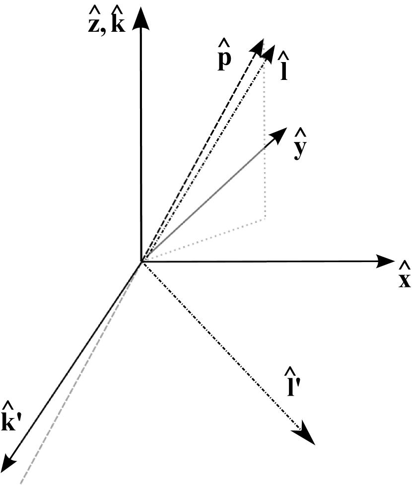
Figure 3: The Compton scattering process as seen in the plasma frame (PF) and in the electron (EF) frame. The PF electron and photon directions before scattering are ${\bf\hat{p}}$ and ${\bf\hat{k}}$, respectively. The EF photon directions of the target and scattered photons are ${\bf\hat{k}}^{\prime}$ and ${\bf\hat{l}}^{\prime}$, respectively. The direction of the scattered photon in the PF is denoted with ${\bf\hat{l}}$.

For each photon, an inverse Compton scattering process is simulated with the following procedure. See Figure 3 for sketches of the scattering process in the plasma and electron frames. We dash all quantities in the EF.
(1) A random number generator is used to draw the direction ${\bf\hat{p}}$ ($\theta_{\rm e},\phi_{\rm e})$ of the scattering electron in the PF. We track the likelihood of an electron-photon interaction by multiplying the Stokes vector of the photon by the factor (1-$\beta\mu_{\rm kp}$). Here, $\beta$ is the velocity of the electron in units of the speed of light and $\mu_{\rm kp}={\bf\hat{k}}\cdot{\bf\hat{p}}$ is the cosine of the angle between the propagation directions of the target photon and the electron.
(2) In the second step, we Lorentz transform the photon’s wave vector and Stokes vector into the EF using

$$\mu_{\rm k^{\prime}p^{\prime}}^{\prime}\,=\,\frac{\mu_{\rm kp}-\beta}{1-\mu_{\rm kp}\beta}$$ (9)

and

$${\bf\hat{k}}^{\prime}\,=\,\mu_{\rm k^{\prime}p^{\prime}}^{\prime}{\bf\hat{p}}+\sqrt{1-\mu_{\rm k^{\prime}p^{\prime}}^{\prime}{}^{2}}\,{\bf\hat{P}}[{\bf\hat{k}},{\bf\hat{p}}].$$ (10)

The photon frequency transforms as

$$\omega^{\prime}\,=\,\gamma(1-\beta\mu_{\rm kp})\omega$$ (11)

with $\gamma=\sqrt{1/(1-\beta^{2})}$ being the Lorentz factor of the electron.

De Young showed that Lorentz boosts do not change the linear and circular polarization properties of a statistical ensemble of photons including the linear and circular polarization degrees (De Young, 1966). As we use a Stokes vector to track the statistical weight of a scattering process and information about the polarization direction, but not to track a beam intensity (radiation power per solid angle, area, and time), the transformed Stokes parameter $i$ is not affected by the Lorentz boosts. We transform the Stokes vector into the coordinate system $C_{\rm kp}\,=\{{\bf\hat{n}}[{\bf\hat{k}}\times{\bf\hat{p}}],{\bf\hat{k}}\}$ with the $y$-axis perpendicular to the (k-p)-plane:

$${\bf s}_{\rm kp}={\rm\bf M}[\phi_{\rm e}]\,\,{\bf s}.$$ (12)

The Stokes vector ${\bf s}_{\rm kp}$ in the PF is identical to the Stokes vector ${\bf s}_{\rm k^{\prime}p}$ defined in the EF with regards to the coordinate system $C_{\rm k^{\prime}p}\,=\{{\bf\hat{n}}[{\bf\hat{k}}^{\prime}\times{\bf\hat{p}}],{\bf\hat{k^{\prime}}}\}$:

$${\bf s}^{\prime}_{\rm k^{\prime}p}\,=\,{\bf s}_{\rm kp}.$$ (13)

This important result follows from the Lorentz invariance of the polarization degree and from symmetry considerations alone. The latter imply that a beam polarized in the (k-p)-plane in the PF will be polarized in the same plane in the EF, because there is no preferred polarization direction perpendicular to the plane. Thus, the invariance of the polarization degree implies that a beam with $q=-x$ and $u=0$ in the PF will have $q=-x$ and $u=0$ in the EF, i.e. that $q$ is Lorentz invariant. The Lorentz invariance of $\Pi$ and $q$ implies the Lorentz invariance of $u$. Equations (6a-c) of (Begelman & Sikora, 1987) imply the same result, but were given without justification.
(3) The third step implements the Compton scattering process in the EF. We denote the wave vector of the scattered photon with $l^{\prime}$, and use a random number generator to draw a random direction for the spatial part of $l^{\prime}$ assuming a constant probability per solid angle. With $\mu_{\rm k^{\prime}l^{\prime}}^{\prime}=$ ${\bf\hat{k}}^{\prime}\cdot{\bf\hat{l}}^{\prime}$, the scattering angle is $\theta_{\rm s}^{\prime}=$ $\arccos{\mu_{\rm k^{\prime}l^{\prime}}^{\prime}}$. We use Compton’s scattering formula $\Delta\lambda=\frac{h}{m_{\rm e}\,c}(1-\mu_{\rm k^{\prime}l^{\prime}}^{\prime})$ to calculate the frequency of the scattered photon:

$$\omega_{\rm s}^{\prime}\,=\,\frac{1}{1+\epsilon^{\prime}\,(1-\mu_{\rm k^{\prime}l^{\prime}}^{\prime})}\omega^{\prime}$$ (14)

where $\epsilon^{\prime}=\hbar\omega^{\prime}/m_{\rm e}c^{2}$ is the target photon energy in the EF in units of the electron rest mass. We can now use the part of Fano’s Compton scattering matrix relevant for linear polarization to calculate the Stokes vector of the scattered photon (McMaster, 1961; Fano, 1949, 1957):

$${\bf s}_{\rm l^{\prime}k^{\prime}}^{\prime}\,=\,{\rm\bf F}[\theta_{\rm s}^{\prime},\epsilon^{\prime},\epsilon_{\rm s}^{\prime}]\,\,{\rm\bf M}[\Delta[C_{\rm k^{\prime}p},C_{\rm l^{\prime}k^{\prime}}]]\,\,{\bf s}_{\rm k^{\prime}p}^{\prime}.$$ (15)

The matrix M transforms the Stokes vector ${\bf s}_{\rm k^{\prime}p}^{\prime}$ into the coordinate frame $C_{\rm l^{\prime}k^{\prime}}=\{{\bf\hat{n}}[{\bf\hat{l}}^{\prime}\times{\bf\hat{k}}^{\prime}],{\bf\hat{l}}^{\prime}\}$ with the $y$-axis perpendicular to the (k^′-l^′)-plane – a prerequisite for using Fano’s matrix. Fano’s matrix F describes Thomson scattering in the Thomson and Klein-Nishina regimes and reads:

$${\rm\bf F}[\theta_{\rm s}^{\prime},\epsilon^{\prime},\epsilon_{\rm s}^{\prime}]\,=\,\left(\frac{\epsilon_{\rm s}^{\prime}}{\epsilon^{\prime}}\right)^{2}\left(\begin{array}[]{ccc}1+{\rm cos}^{2}\theta_{\rm s}^{\prime}+(\epsilon^{\prime}-\epsilon_{\rm s}^{\prime})(1-\cos{\theta_{\rm s}^{\prime}})&{\rm sin}^{2}\theta_{\rm s}^{\prime}&0\\ {\rm sin}^{2}\theta_{\rm s}^{\prime}&1+{\rm cos}^{2}\theta_{\rm s}^{\prime}&0\\ 0&0&2\cos{\theta_{\rm s}^{\prime}}\end{array}\right)$$ (16)

with $\epsilon_{\rm s}^{\prime}=\hbar\omega_{\rm s}^{\prime}/m_{\rm e}c^{2}$ being the energy of the scattered photon in the EF in units of the electron rest mass. We did not include here the numerical factor $r_{0}{}^{2}/2$ (with $r_{0}$ being the classical electron radius) in the definition of F, as we are not interested in absolute fluxes in the following. Note that Fano’s matrix accounts for the statistical weight of the scattering process by modifying the $i$-component of the Stokes vector; the resulting Stokes vector is defined relative to $C_{\rm l^{\prime}k^{\prime}}$.
(4) The final step consists in back-transforming the results into the PF. The cosine of the angle between the scattered photon direction and the electron direction $\mu_{\rm l^{\prime}p^{\prime}}^{\prime}=$${\bf\hat{l}}^{\prime}\cdot{\bf\hat{p}}^{\prime}$ transforms as follows into the PF:

$$\mu_{\rm lp}\,=\,\frac{\mu_{\rm l^{\prime}p^{\prime}}^{\prime}+\beta}{1+\mu_{\rm l^{\prime}p^{\prime}}^{\prime}\beta}.$$ (17)

The scattered photon direction in the PF is

$${\bf\hat{l}}\,=\,\mu_{\rm lp}{\bf\hat{p}}+\sqrt{1-\mu_{\rm lp}{}^{2}}\,{\bf\hat{P}}[{\bf\hat{l}}^{\prime},{\bf\hat{p}}].$$ (18)

The PF frequency of the scattered photon is

$$\omega_{\rm s}\,=\,\gamma(1+\beta\mu_{\rm l^{\prime}p^{\prime}}^{\prime})\omega_{\rm s}^{\prime}.$$ (19)

After inferring the Stokes vector of the scattered photon into the coordinate system $C_{\rm l^{\prime}p}=\{{\bf\hat{n}}[{\bf\hat{l}}^{\prime}\times{\bf\hat{p}}],{\bf\hat{l}}^{\prime}\}$ with the $y$-axis perpendicular to the (l^′-p)-plane:

$${\bf s}_{\rm l^{\prime}p}^{\prime}\,=\,{\rm\bf M}[\Delta[C_{\rm l^{\prime}k^{\prime}},C_{\rm l^{\prime}p}]]\,\,{\bf s}_{\rm l^{\prime}k^{\prime}}^{\prime},$$ (20)

we Lorentz transform the Stokes vector into the PF relative to $C_{\rm lp}=\{{\bf\hat{n}}[{\bf\hat{l}}\times{\bf\hat{p}}],{\bf\hat{l}}\}$

$${\bf s}_{\rm lp}\,=\,{\bf s}_{\rm l^{\prime}p}^{\prime}.$$ (21)

Finally, we compute the Stokes vector relative to the coordinate system $C_{\rm lk}=\{{\bf\hat{P}}[{\bf\hat{k}},{\bf\hat{l}}],{\bf\hat{l}}\}$ with the $y$-axis aligned with the projection of the target photon’s propagation direction in the sky:

$${\bf s}_{\rm lk}\,=\,{\rm\bf M}[\Delta[C_{\rm lp},C_{\rm lk}]]\,\,{\bf s}_{\rm lp}.$$ (22)

2.3 Simulation of SSC emission

The simulation of SSC emission from electron and photon powerlaw distributions proceeds along similar lines. The calculations assume a uniform magnetic field B oriented at an angle $\vartheta_{\rm B}$ to the line of sight. A random photon propagation direction ${\bf\hat{k}}$ is drawn assuming a constant probability per solid angle. Subsequently, we generate a random photon frequency between $\omega_{1}$ and $\omega_{2}$ from a power law distribution with $dN_{\gamma}/dE_{\gamma}\propto E_{\gamma}^{-(\alpha+1)}$. Similarly, an electron Lorentz factor is drawn from a power law distribution with $dN_{\rm e}/d_{\gamma}\propto\gamma^{-p}$. The initial Stokes vector is set to

$${\bf s}_{\rm kB}\,=\,(1-\beta\mu_{\rm kp})\,{\rm sin}^{\alpha+1}{\theta_{\rm B}}\,\left(\begin{array}[]{c}1\\ \Pi_{\rm S}\\ 0\end{array}\right)$$ (23)

with $\theta_{\rm B}$ being the angle between ${\bf\hat{k}}$ and the magnetic field B and $\mu_{\rm kp}={\bf\hat{k}}\cdot{\bf\hat{p}}$ as above. The two multiplicative factors account for the relative likelihood of a electron-photon interaction and for the scaling of the synchrotron emissivity with $\theta_{\rm B}$ (Ginzburg & Syrovatskii, 1965). We assume that the emission is linearly polarized along the ${\bf\hat{q}}_{+}$-direction and the value of the $q$-parameter gives the polarization degree of synchrotron emission with a power law index $\alpha$:

$$\Pi_{\rm S}\,=\,\frac{1+\alpha}{\alpha+5/3}.$$ (24)

As synchrotron emission is polarized perpendicular to the B-field, ${\bf s}_{\rm kB}$ is defined with regards to the coordinate system $C_{\rm kB}=\{{\bf\hat{n}}[{\bf\hat{k}}\times{\bf B}],{\bf\hat{k}}\}$. The rest of the procedure is now equivalent to the one described in Steps (2)-(4) above with the modification that the Stokes vector ${\bf s}_{\rm kp}$ is now given by

$${\bf s}_{\rm kp}\,=\,{\rm\bf M}[\Delta[C_{\rm kB},C_{\rm kp}]]\,\,{\bf s}_{\rm kB}.$$ (25)

At the very end of the calculation, we compute the Stokes vector relative to a coordinate system $C_{\rm lB}=\{{\bf\hat{P}}[{\bf B},{\bf\hat{l}}],{\bf\hat{l}}\}$ with the $y$-axis along the B-field direction in the PF projected onto the sky:

$${\bf s}_{\rm lB}\,=\,{\rm\bf M}[\Delta[C_{\rm lp},C_{\rm lB}]]\,\,{\bf s}_{\rm lp}.$$ (26)

3 Analytical and numerical results

3.1 Analytical results derived by BCS and BS

We continue to use the same naming conventions as in the previous section. The frequency of an inverse Compton scattered photon can be computed from Equations (11), (14), and (19). In the Thomson regime $\epsilon^{\prime}\rightarrow 0$ we get

$$\omega_{\rm s}\,=\gamma^{2}(1-\beta\mu_{\rm kp})(1+\beta\mu^{\prime}_{\rm l^{\prime}p^{\prime}})\omega.$$ (27)

This equation gives the following minimum and maximum scattered photon frequencies as function of $\gamma$, $\omega$, and $\mu_{\rm kp}$:

$$\omega_{\rm min}\,=\frac{1-\beta\mu_{\rm kp}}{2}\omega$$ (28)

and

$$\omega_{\rm max}\,=2\gamma^{2}(1-\beta\mu_{\rm kp})\omega,$$ (29)

respectively. We will see below, that $\omega_{\rm max}$ sets a useful scale to characterize the frequency dependence of the intensity and polarization degree of inverse Compton emission.

From the last equation we infer that the minimum Lorentz factor $\gamma_{\rm min}$ required to produce photons of frequency $\omega_{\rm s}$ is for $\gamma\gg 1$ and $\beta\approx 1$:

$$\gamma_{\rm min}\,=\,\sqrt{\frac{1}{2}\frac{\omega_{\rm s}}{\omega}\frac{1}{(1-\mu_{\rm kp})}}.$$ (30)

BCS and BS derived an expression for the intensity $J_{{\bf\hat{\boldsymbol{\varepsilon}}}_{\rm s}}$ (energy emitted per unit time, unit volume and unit frequency interval) of a unidirectional monoenergetic photon beam polarized along the vector ${\bf\hat{\boldsymbol{\varepsilon}}}$ scattered by an isotropic electron population in the direction ${\bf\hat{l}}$ into a state of linear polarization defined by the polarization vector ${\bf\hat{\boldsymbol{\varepsilon}}}_{\rm s}$:

$$J_{{\bf\hat{\boldsymbol{\varepsilon}}}_{\rm s}}\,=\,K\,\gamma_{\rm min}\frac{\omega}{\omega_{\rm s}}\left\{\left[{\bf\hat{\boldsymbol{\varepsilon}}}\cdot{\bf\hat{\boldsymbol{\varepsilon}}}_{\rm s}+\frac{({\bf\hat{k}}\cdot{\bf\hat{\boldsymbol{\varepsilon}}}_{\rm s})({\bf\hat{l}}\cdot{\bf\hat{\boldsymbol{\varepsilon}}})}{1-({\bf\hat{k}}\cdot{\bf\hat{l}})}\right]^{2}\,(\Sigma_{1}+\Sigma_{2})+\Sigma_{2}\right\}$$ (31)

with $K\equiv$ $\frac{1}{2}h\,c\,r_{0}{}^{2}\,\rm cm^{-3}$ and $\gamma_{\rm min}$ as defined above. The factors $\Sigma_{1}$ and $\Sigma_{2}$ depend on the electron energy spectrum:

$$\Sigma_{1}\,=\int_{0}^{1}\,m(\gamma)\,\left(x^{2}-\frac{1}{x^{2}}+2\right)dx$$ (32)

$$\Sigma_{2}\,=\int_{0}^{1}\,m(\gamma)\,\frac{(1-x)^{2}}{x^{2}}dx.$$ (33)

The function $m$ depends on $dn_{\rm e}/d\gamma$, the differential electron spectrum per unit volume, as:

$$m(\gamma)=\frac{dn_{\rm e}}{d\gamma}\gamma^{-2},$$ (34)

and $x$ is defined as

$$x=\frac{\gamma_{\rm min}}{\gamma}.$$ (35)

Summing Equation (31) over two orthogonal polarization directions gives the total intensity of the inverse Compton scattered radiation:

$$J_{{\bf\hat{\boldsymbol{\varepsilon}}}_{\rm s}}+J_{{\bf\hat{\boldsymbol{\varepsilon}}}_{\rm s,\perp}}\,=\,K\,\gamma_{\rm min}\,\frac{\omega}{\omega_{\rm s}}(\Sigma_{1}+3\,\Sigma_{2}).$$ (36)

BCS evaluated the linear polarization fraction for three exemplary cases with different initial polarization directions relative to the scattering plane (${\bf\hat{\boldsymbol{\varepsilon}}}_{\rm s}$ parallel, at 45^∘, and perpendicular to the scattering plane). The main results of the calculations are:
(i) The intensity of the inverse Compton radiation is independent of the polarization degree and direction of the target photon beam, and does not depend on the scattering direction.
(ii) The linear polarization degree of the inverse Compton radiation depends on the degree but not the direction of the polarization of the target photons, and does not depend on the scattering direction. For a 100% polarized target beam, the linear polarization degree of the inverse Compton scattered radiation is

$$\Pi_{\rm BCS}\,=\,\frac{\Sigma_{1}+\Sigma_{2}}{\Sigma_{1}+3\,\Sigma_{2}}.$$ (37)

Note that although $\Sigma_{1}<0$ is possible, the combinations $\Sigma_{1}+\Sigma_{2}$ and $\Sigma_{1}+3\Sigma_{2}$ are equal or larger than zero. BCS evaluated $\Pi_{\rm BCS}$ analytically for powerlaw electron distributions and numerically for the case of SSC emission.
(iii) In contrast to Thomson scattering by stationary electrons, Inverse Compton scattering by non-thermal electron plasmas does not create polarization, and an initially unpolarized beam stays unpolarized after scattering. This result implies that if inverse Compton scattering reduces the polarization degree of a 100% polarized target beam to $\Pi_{1}$, it will reduce the polarization degree of a target beam with a polarization degree of $\Pi_{2}$ to a net-polarization of $\Pi_{1}\,\Pi_{2}$.

3.2 Additional analytical results

Equation (31) allows us to derive a closed expression for the polarization direction of the inverse Compton scattered radiation. The latter is given by the unit vector ${\bf\hat{\boldsymbol{\varepsilon}}}_{\rm s}$ which maximizes the term in square brackets of Equation (31) with the constraining condition that ${\bf\hat{\boldsymbol{\varepsilon}}}_{\rm s}\perp{\bf\hat{l}}$. If we pull out the vector ${\bf\hat{\boldsymbol{\varepsilon}}}_{\rm s}$ from the term in Equation (31) in square brackets, we see that the condition is equivalent to minimizing the angular distance between ${\bf\hat{\boldsymbol{\varepsilon}}}_{\rm s}$ and the vector

$${\bf v}\,=\,{\bf\hat{\boldsymbol{\varepsilon}}}+\frac{{\bf\hat{l}}\cdot{\bf\hat{\boldsymbol{\varepsilon}}}}{1-({\bf\hat{k}}\cdot{\bf\hat{l}})}\,{\bf\hat{k}}.$$ (38)

The angular distance is minimized for the projection of ${\bf v}$ onto the plane perpendicular to ${\bf\hat{l}}$. The polarization vector is thus given by the expression

$${\bf\hat{\boldsymbol{\varepsilon}}}_{\rm s}\,=\,{\bf\hat{P}}[{\bf v},{\bf\hat{l}}].$$ (39)

Using this expression, it can be shown in a somewhat tedious calculation that the polarization angle $\chi=\arccos{({\bf\hat{\boldsymbol{\varepsilon}}}_{\rm s}\cdot{\bf\hat{P}}[{\bf\hat{k}},{\bf\hat{l}}])}$ equals the angle between the initial polarization direction and the projection of ${\bf\hat{l}}$ onto the plane perpendicular to ${\bf\hat{k}}$:

$$\chi\,=\,\arccos{({\bf\hat{\boldsymbol{\varepsilon}}}\cdot{\bf\hat{P}}[{\bf\hat{l}},{\bf\hat{k}}])}.$$ (40)

While Equation (39) gives the polarization direction, Equation (40) gives only the absolute value of $\chi$ but not the sign of $\chi$. With regards to Figure 1, the polarization angle $\chi$ is $\pi/2-\phi_{\rm e}$. Note that the polarization direction does not depend on the observed frequency.

The BCS equations allow us to derive the frequency dependence of the intensity and polarization degree of the inverse Compton emission from monoenergetic electrons. The differential energy spectrum of a monoenergetic electron beam normalized to one electron per cm³ is

$$\frac{dn_{\rm e}}{d\gamma}\,=\,\delta(\gamma-\gamma_{0})\,\rm cm^{-3}.$$ (41)

The integrands in Equations (32) and (33) only contribute for

$$x_{0}\,\equiv\,\frac{\gamma_{\rm min}}{\gamma_{0}}.$$ (42)

We get after some algebra

$$\Sigma_{1}\,=\,\frac{2-\frac{1}{x_{0}^{2}}+x_{0}^{2}}{\gamma_{0}{}^{3}}$$ (43)

and

$$\Sigma_{2}\,=\,\frac{(1-x_{0}{\,}^{2})^{2}}{x_{0}\,\gamma_{0}{}^{3}}.$$ (44)

Note that both parameters $\Sigma_{1}$ and $\Sigma_{2}$ depend through $x_{0}$ (and thus through $\gamma_{\rm min}$) on the observed frequency $\omega_{\rm s}$. We obtain the total intensity

$$J\,=\,K\,\frac{\omega_{\rm s}}{\omega}\,\frac{2\left(1-2x_{0}{}^{2}+2x_{0}{}^{4}\right)}{\gamma_{0}{}^{2}}$$ (45)

and the polarization degree

$$\Pi_{\rm BCS}\,=\,\frac{x_{0}{}^{4}}{1-2x_{0}{}^{2}+2x_{0}{}^{4}}.$$ (46)

We now introduce the dimensionless variable $y$ as the observed frequency in units of the maximum frequency $\omega_{\rm max}(\gamma_{0},\mu_{\rm kp})$ which electrons of Lorentz factor $\gamma_{0}$ emit in a certain direction:

$$y\,=\,\frac{\omega_{\rm s}}{\omega_{\rm max}}.$$ (47)

The intensity scales with $y$ as

$$J\,\propto\,y\frac{1-2y+2y^{2}}{\gamma_{0}{}^{2}}.$$ (48)

We infer a differential photon number per unit frequency interval of

$$\rho_{\gamma_{0}}\,\equiv\,\frac{dN_{\gamma}}{d\omega_{\rm s}}\,=\,\frac{dN_{\gamma}}{dy}\frac{dy}{d\omega_{\rm s}}\,\,=\,\frac{3(1-2y+2y^{2})}{2\,\omega_{\rm max}}$$ (49)

where we introduced the normalization factor $3/(2\,\omega_{\rm max})$ so that $\int_{\omega_{\rm min}}^{\omega_{\rm max}}\rho_{\gamma_{0}}d\omega_{\rm s}=1$ for $\omega_{\rm min}\approx 0$.

The polarization degree as function of $y$ is

$$\Pi_{\gamma_{0}}\,=\,\frac{y^{2}}{1-2y+2y^{2}}.$$ (50)

Equations (49) and (50) give the intensity and polarization fraction of the inverse Compton emission from monoenergetic electrons and can be used as integration kernel to predict the spectral shape and polarization properties of the inverse Compton emission from more complicated electron distributions.

3.3 Comparison of numerical and analytical results in the Thomson Regime

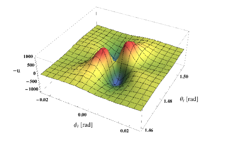
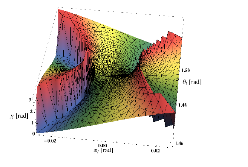
Figure 4: Distribution of the Stokes $i$, $q$ and $u$ parameters and the polarization direction $\chi$ of the inverse Compton emission from a monoenergetic unidirectional electron beam ($\gamma=100$, $(\theta_{\rm e},\phi_{\rm e})=$ $(85^{\circ},0)$) scattering a monoenergetic unidirectional target photon beam propagating along the $z$-axis and polarized along the $y$-axis ($\omega=10^{12}$ Hz, ${\bf\hat{k}}=(0,0,1)$, ${\bf s}=(1,1,0)$) as function of the polar coordinates of the scattered photon direction ${\bf\hat{l}}$. $\chi$ is measured relative to ${\bf\hat{q}}_{+}$ aligned with the projection of ${\bf\hat{k}}$ onto the sky.

It is instructive to look at the numerical results for a monoenergetic unidirectional photon beam scattering off a monoenergetic unidirectional electron beam. Figure 4 shows the Stokes parameters $i$, $q$, and $u$ and the polarization direction $\chi$ for an electron beam with $\theta_{\rm e}=85^{\circ}$, $\phi_{\rm e}=0^{\circ}$ and $\gamma=100$ impinging on a photon beam with frequency $\omega=10^{12}$ Hz incident along the $z$-axis (${\bf\hat{k}}={\bf\hat{z}}$), 100% polarized along the $y$-axis with an initial Stokes vector ${\bf s}=(1,1,0)$. As explained in the previous section, the polarization direction is measured clockwise from the direction of ${\bf\hat{k}}$ in the sky when looking into the inverse Compton scattered beam.

In the electron rest frame, the intensity of the Thomson scattered photons resembles the torus-shaped intensity emitted by a Hertzian dipole. After back-transformation into the PF, the intensity of the inverse Compton emission shows two poles with zero intensity at an angular distance of $2/\gamma$ from each other bracketing the high-intensity radiation emitted in the direction of the electron direction. The $q$ and $u$ distributions look complicated, but encode simple information: the inverse Compton emission from monoenergetic unidirectional electrons is everywhere polarized to 100%, and beyond the poles of the Hertzian dipole, the polarization direction exhibits a smooth rotation with a periodicity of $\pi/2$ around the maximum-intensity direction. The frequencies of the scattered photons (not shown here) are approximately evenly distributed between $\omega_{\rm min}$ and $\omega_{\rm max}$ ($dN_{\gamma}/d\omega_{\rm s}\approx const$).

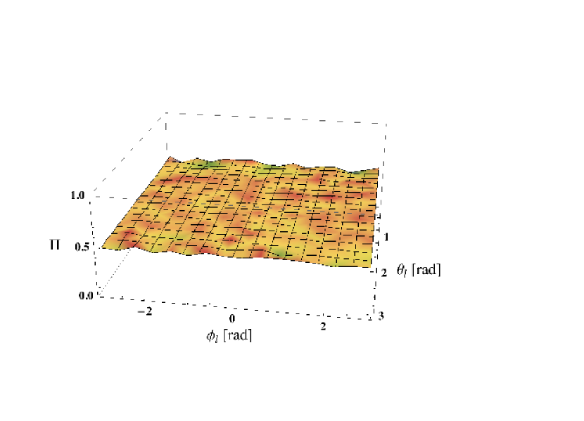
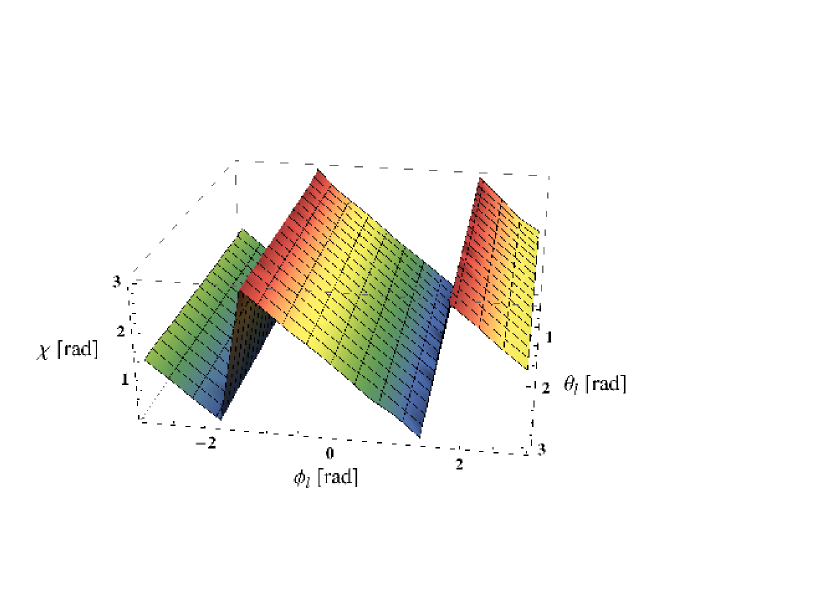
Figure 5: Polarization degree $\Pi$ and polarization direction $\chi$ of the inverse Compton emission from a monoenergetic isotropic electron distribution ($\gamma=100$) scattering a monoenergetic unidirectional target photon beam ($\omega=10^{12}$ Hz, ${\bf\hat{k}}=$(0,0,1), ${\bf s}=(1,1,0)$) as function of the polar coordinates of the scattered photon direction ${\bf\hat{l}}$. $\chi$ is measured relative to ${\bf\hat{q}}_{+}$ aligned with the projection of ${\bf\hat{k}}$ onto the sky.

For an isotropic electron configuration, electrons with initial directions within a few $\gamma^{-1}$ from the observed direction contribute $i$, $q$, and $u$-patterns as shown in Figure 4. It is clear that summing up positive $i$-values and positive and negative $q$ and $u$-values will result in an overall polarization degree smaller than unity. Figure 5 shows the intensity, polarization degree and polarization direction for an isotropic electron distribution with all other parameters being the same as in the previous example. The angular distribution of the inverse Compton emission (not shown here) is constant up to a dependence $\propto(1-\beta\mu_{\rm kl})$ (with $\mu_{\rm kl}={\bf\hat{k}}\cdot{\bf\hat{l}}$) owing to the relative motion of the electrons and photons. Figure 5 shows the polarization degree and polarization direction for all scattering directions. The simulations show that the polarization degree is $\Pi=0.5$ independent of the scattering direction and that the polarization direction depends on ${\bf\hat{k}}$, ${\bf\hat{\boldsymbol{\varepsilon}}}$, and ${\bf\hat{l}}$ as predicted by Equation (39).

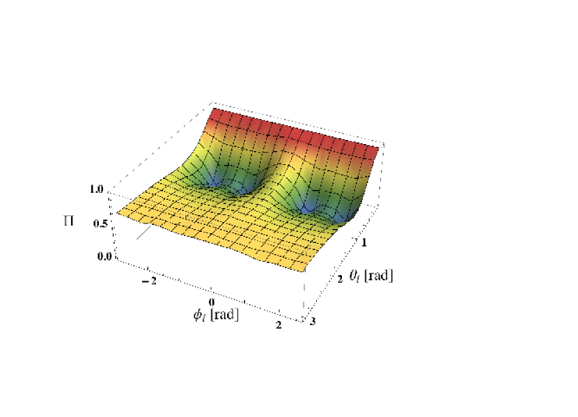
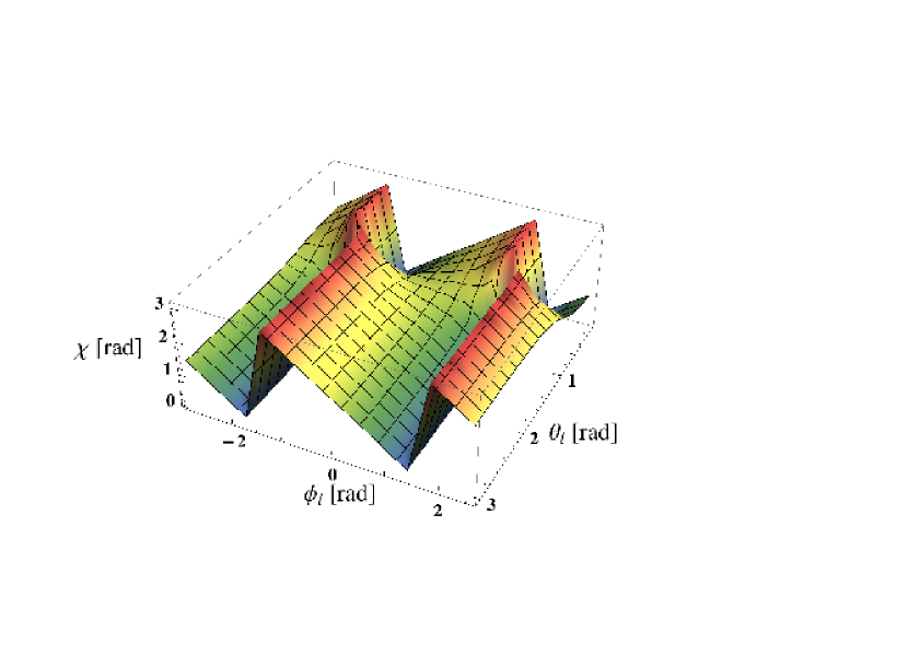
Figure 6: Same as Figure 5, but for electrons with Lorentz factor $\gamma=2$.

For mildly relativistic electrons, the polarization properties do depend on the scattering direction. As an example, Figure 6 shows the same as the previous figure, but for $\gamma=2$. At an angle $\theta_{\rm l}\approx$ 60^∘ to the target photon beam, the polarization degree dips and the dependence of $\chi$ on the azimuthal angle of ${\bf\hat{l}}$ reverses. The main difference between the mildly relativistic and highly relativistic cases is that in the latter ${\bf\hat{p}}$ and ${\bf\hat{k}}^{\prime}$ are almost always nearly antiparallel while in the former, the photons approach the electrons from a wide range of directions. In the mildly relativistic case, the polarization direction of the incident photon is thus not “rotated” around an axis perpendicular to the ${\bf\hat{p}}$-${\bf\hat{l}}$ plane.

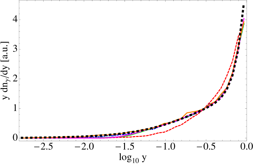
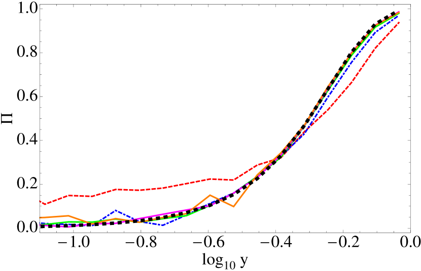
Figure 7: Frequency dependence of the intensity (left panel) and polarization degree (right panel) of the inverse Compton emission from a monoenergetic isotropic electron population scattering a monoenergetic unidirectional photon beam. All parameter values are the same as in Figure 4, except $\gamma=2$ (dashed red lines), $\gamma=5$ (dot-dashed blue lines), $\gamma=10$ (solid green lines), $\gamma=20$ (solid magenta lines), and $\gamma=100$ (solid orange lines). The dotted black lines display the analytical results from Equations (49) and (50). The frequencies are given as $y=\omega_{\rm s}/\omega_{\rm max}$ in units of the maximum frequency for Thomson processes. The results are shown for photons emitting along the direction $(\theta_{\rm l},\phi_{\rm l})=$ $(85^{\circ},0)$. The plotting range of the right panel is restricted to the range where the statistical errors on the polarization degree are sufficiently small (a color version of this figure is available in the online journal).

In the next step, we compare the frequency dependence of the intensity and polarization degree and direction with the theoretical predictions from Equations (49), (50), and (38-39), respectively. We consider the radiation scattered into the direction ${\bf\hat{l}}$ with the polar coordinates $(85^{\circ},0^{\circ})$ for $\gamma$-values of 2, 5, 10, 20, and 100. Figure 7 shows that Equation (49) describes the frequency dependence extremely well except for mildly relativistic electrons with $\gamma=2$. Furthermore, Equation (50) gives a good description of the polarization degree – again, except for $\gamma=2$. Additional simulations at higher $\gamma$-values ($\gamma=$ 2,500, 12,500, and 62,500) show intensity and polarization degree distributions identical to the one shown for $\gamma=$100. We also verified that the polarization direction (not shown here) is independent of frequency.

The case of a powerlaw distribution of electrons ($dN_{\rm e}/d\gamma\propto\gamma^{-p}$ from $\gamma_{1}$ to $\gamma_{2}$) scattering off monoenergetic unidirectional photons is discussed in the paper of BCS. In the region where the emitted energy spectrum is a power-law, the polarization degree is predicted to be

$$\Pi_{\rm pl}\,\approx\,\frac{(1+p)(3+p)}{11+4p+p^{2}}.$$ (51)

Equations (49) and (49) give a frequency dependent polarization degree of

$$\Pi_{\rm pl}\,=\,\frac{\int_{\gamma_{1}{}^{\prime}}^{\gamma_{2}}\,\frac{dN_{\rm e}}{d\gamma}\,\rho_{\gamma_{0}}\,\Pi_{\gamma_{0}}\,d\gamma_{0}}{\int_{\gamma_{1}{}^{\prime}}^{\gamma_{2}}\,\frac{dN_{\rm e}}{d\gamma}\,\rho_{\gamma_{0}}\,d\gamma_{0}}$$ (52)

with $\gamma_{1}{}^{\prime}={\rm Max}(\gamma_{1},\gamma_{\rm min})$. The equation is valid for $\gamma_{\rm min}<\gamma_{2}$; no emission is found at frequencies with $\gamma_{\rm min}>\gamma_{2}$. For $\gamma_{1}<\gamma_{\rm min}$ and $\gamma_{2}\rightarrow\infty$, we recover Equation (51).

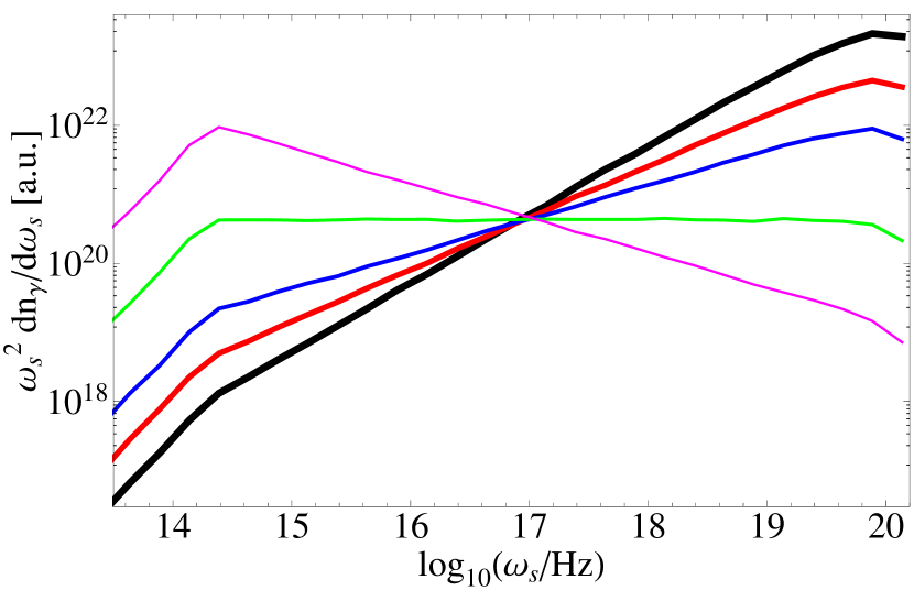
Figure 8: Intensity per logarithmic energy interval (left panel) and polarization degree (right panel) of the inverse Compton emission from isotropic power law electron populations ($dN_{\rm e}/d\gamma\propto\gamma^{-p}$ from $\gamma_{1}=10$ to $\gamma_{2}=10^{4}$) scattering a monoenergetic unidirectional target photon beam ($\omega=10^{12}$ Hz, ${\bf\hat{k}}=$(0,0,1), s=(1,1,0)) into the direction $(\theta_{\rm l},\phi_{\rm l})=$ $(85^{\circ},0)$. The thick to thin solid lines display the simulation results for electron spectral indices of $p=$ 1.01, 1.5, 2, 3, 4. In the right panel, the dotted lines show the semi-analytical results from Equation (52).

Figure 8 compares the prediction from Equation (52) with simulated results for $\gamma_{1}=10$, $\gamma_{2}=10,000$, and electron indices $p$ between 1.01 and 4. The energy spectra of the inverse Compton emission indicate three regimes: a low-frequency regime with $\gamma_{\rm min}<\gamma_{1}$, a power law regime starting at $\gamma_{\rm min}$ $\stackrel{{\scriptstyle>}}{{\scriptstyle\sim}}$$\gamma_{1}$, and a high-frequency regime with $\gamma_{\rm min}\rightarrow\gamma_{2}$. In the low-frequency regime the polarization degree is low as the emission is produced at low $y$-values. In the power-law regime, the polarization is independent of frequency and agrees well with Equations (51) and (52). The softer the energy spectrum, the higher is the polarization degree. In the high-frequency regime, the polarization increases towards $\Pi=1$ as $\omega_{\rm s}\rightarrow\omega_{\rm max}(\gamma_{2})$ because the emission is produced at $y$-values close to 1. The results validate the predictive power of Equation (51) for the power law regime, and of Equation (52) for all frequencies.

We now turn our attention to the polarization of SSC emission from an isotropic electron population emerged in an uniform magnetic field B. We assume that the electron and synchrotron number densities are well described by power law distributions $dN_{\rm e}/d\gamma\propto\gamma^{-p}$ and $dN_{\gamma}/d\omega\propto\omega^{-(\alpha+1)}$ over the relevant energy and frequency ranges. The main objective of our discussion is to explain the polarization degree of the SSC emission from the polarization properties of the synchrotron emission and the general results concerning the depolarization effect of inverse Compton processes described above.

As discussed in Section 2.3, the intensity of the synchrotron emission is proportional to $\sin^{\alpha+1}\,\theta_{\rm B}$, and its polarization degree is $\Pi_{\rm S}$. In the power-law regime of the SSC radiation, the inverse Compton scattering reduces the polarization degree of synchrotron photons of a certain fixed frequency and propagation direction by the factor $\Pi_{\rm pl}$. As the polarization direction of the inverse Compton emission depends on the propagation direction and polarization direction of the synchrotron photons, the net-polarization degree of the emerging SSC emission will be lower than $\Pi_{\rm pl}\Pi_{\rm S}$ and we write

$$\Pi_{\rm SSC}\,\approx\,\eta\,\Pi_{\rm pl}\,\Pi_{\rm S}.$$ (53)

The factor $\eta$ depends on the angle $\vartheta_{\rm B}$ between the magnetic field and the line of sight, because the magnetic field direction determines the intensity and polarization pattern of the synchrotron emission. Furthermore, $\eta$ depends on the spectral index $\alpha$ of the synchrotron emission because of Doppler boosting effects.

We can derive an estimate for $\eta$ in the following way. Relative to the coordinate system $C_{\rm lB}$ with the $y$-axis parallel to the B-field projected onto the plane of the sky and the $z$-axis pointing towards the observer, the $u$-parameter of the SSC radiation vanishes owing to the symmetry of the problem. The factor $\eta$ is then proportional to the absolute value of the $q$-parameter and can be computed by integrating the $q$-parameter over the angular distribution of the synchrotron emission. Note that ${\bf\hat{p}}$ is approximately parallel to ${\bf\hat{l}}$ for most of the contributing electrons. The expression for $\eta$ reads:

$$\eta\,=\,\frac{\left|\,\int\,d\Omega_{{\bf\hat{k}}}\,(1-\beta\mu_{\rm kp})^{\alpha+1}\,(\sin{\theta_{\rm B}})^{\alpha+1}\,\cos{2\,\chi}\,\right|}{\int\,d\Omega_{{\bf\hat{k}}}\,(1-\beta\mu_{\rm kp})^{\alpha+1}\,(\sin{\theta_{\rm B}})^{\alpha+1}}.$$ (54)

The integrals run over the directions ${\bf\hat{k}}$ of the synchrotron photons. The first two factors of the integrands are weighting factors. One power of $(1-\beta\mu_{\rm kp})$ accounts for the dependence of the Compton scattering probability on the relative velocities of the photons and electrons. The additional power $\alpha$ stems from the fact that the synchrotron photons have an EF frequency $\omega^{\prime}\propto$ $(1-\beta\mu_{\rm kp})$ according to Equation (11), and the number of target photons available at a certain $\omega^{\prime}$ in the EF scales proportional to $\frac{dN(\omega^{\prime})}{d\omega^{\prime}}=\frac{dN\left(\omega(\omega^{\prime})\right)}{d\omega}\frac{d\omega}{d\omega^{\prime}}$ $\propto$ $(1-\beta\mu_{\rm kp})^{\alpha}$. The factor $(\sin{\theta_{\rm B}})^{\alpha+1}$ accounts for the dependence of the synchrotron emissivity on the angle $\theta_{\rm B}$ between ${\bf\hat{k}}$ and B. $\chi$ is the polarization direction of the inverse Compton scattered emission computed with the help of Equation (38), and we made use of the identity $q=\cos{2\chi}$ from Equation (1). The denominator normalizes the expression. The numerical evaluation of the integral in the nominator gives negative values, corresponding to parallel synchrotron and SSC polarization directions – perpendicular to the projection of the magnetic field in the PF onto the sky.

A frequency dependent estimate of the polarization degree can be derived from Equations (49) and (50):

$$\Pi_{\rm SSC}(\omega_{\rm s})\,=\,\frac{|q|}{i}\,=\,\frac{\left|\,\int\,d\Omega_{{\bf\hat{k}}}\,\int_{\omega_{1}}^{\omega_{2}}\,d\omega\int_{\gamma^{\prime}_{1}}^{\gamma_{2}}\,d\gamma_{0}\,\frac{dN_{\rm e}}{d\gamma}\,\frac{dN_{\gamma}}{d\omega}\,(1-\beta\mu_{\rm kp})\,(\sin{\theta_{\rm B}})^{\alpha+1}\,\rho_{\gamma_{0}}\,\Pi_{\rm S}\,\Pi_{\gamma_{0}}\,\cos{2\,\chi}\,\right|}{\int\,d\Omega_{{\bf\hat{k}}}\,\int_{\omega_{1}}^{\omega_{2}}\,d\omega\int_{\gamma^{\prime}_{1}}^{\gamma_{2}}\,d\gamma_{0}\,\frac{dN_{\rm e}}{d\gamma}\,\frac{dN_{\gamma}}{d\omega}\,(1-\beta\mu_{\rm kp})\,(\sin{\theta_{\rm B}})^{\alpha+1}\,\rho_{\gamma_{0}}}$$ (55)

The integrals run over the directions of the synchrotron photons, the synchrotron photon frequencies and the electron Lorentz factors. Only electrons with Lorentz factors $\gamma\geq$ $\gamma^{\prime}_{1}\,=$ Max($\gamma_{1},\gamma_{\rm min}$) contribute and we set the value of the inner integral to zero if $\gamma^{\prime}_{1}\,>\gamma_{2}$. The first three factors of the integrand weight according to the electron and photon number densities and the interaction probability, the fourth factor is proportional to the synchrotron emissivity, and the fifth factor gives the photon density of the inverse Compton emission. In the integral of the nominator we multiply all these weighting factors with the fractional polarization of the synchrotron photons and the inverse Compton emission, and multiply with the contribution of the considered emission to the $q$-parameter at frequency $\omega_{\rm s}$.

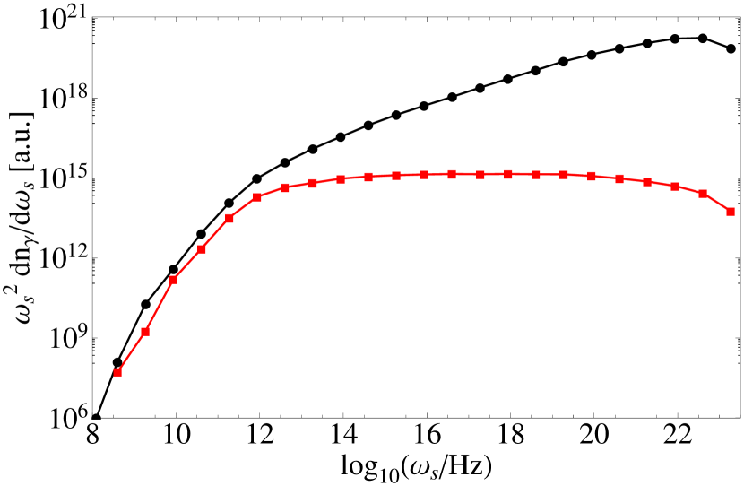
Figure 9: Intensity per logarithmic energy interval (left panel) and polarization degree (right panel) of the SSC emission from isotropic power law electron populations ($dN_{\rm e}/d\gamma\propto\gamma^{-p}$ from $\gamma_{1}=10$ to $\gamma_{2}=10^{5}$) scattering synchrotron emission ($dN_{\gamma}/d\omega\propto\omega^{-(\alpha+1)}$ from $\omega_{1}=10^{9}$ Hz to $\omega_{2}=10^{13}$ Hz) from a B-field at 85^∘ to the line of sight. Numerical results are reported for $\alpha=0.5$ and $p=2$ (circles), and $\alpha=1$ and $p=3$ (squares). The dotted lines in the right panel present the semi-analytical results from Equation (55). The dashed lines are the semi-analytical results from BS and the dashed-dotted lines report the numerical results from CM. Both papers do not give frequency resolved results.

The numerical evaluation of the SSC polarization follows the description in Section 2.3. Figure 9 presents the intensity and polarization degrees of the SSC emission for $\omega_{1}=10^{9}$ Hz, $\omega_{2}=10^{13}$ Hz, $\gamma_{1}=10$, $\gamma_{2}=10^{5}$, for ($\alpha=0.5,\,p=2$) and $(\alpha=1,\,p=3)$, and various $\vartheta_{\rm B}$-values. After low values at the lowest frequencies, the polarization degree of the SSC emission $\Pi_{\rm SSC}$ reaches a rather stable plateau with a gradual increase before an eventual peak at the highest frequencies. The polarization degrees calculated with Equation (55) (Figure 9, right panel, dotted lines) agree well with the results from the Monte Carlo simulations. The right panel also shows the SSC polarization degrees presented in BS and CM. Whereas the polarization degrees of BS agrees well with our calculations, those of CM deviate by up to $\sim$15%. We explain the disagreement with the fact that CM measure the polarization degrees at frequencies where electrons with $\gamma<10$ still play an important role.

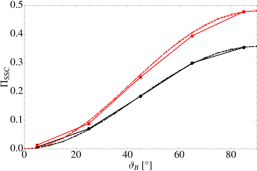
Figure 10: Polarization degree of the SSC emission as function of the angle $\vartheta_{\rm B}$ between the magnetic field and the line of sight for $\alpha=1$ and $p=3$ (squares) and $\alpha=0.5$ and $p=2$ (circles), evaluated between $10^{16}$ and $10^{18}$ Hz. The dashed line displays the expectation from Equation (55), and the dotted line shows the results from Equations (53) and (54).

Figure 10 compares the $\vartheta_{\rm B}$-dependence of the emitted radiation with the predictions of Equations (53-55). The Monte Carlo simulations and Equation (55) give frequency dependent polarization degrees, and we used here the polarization degrees averaged from 10¹⁶ to 10¹⁸ Hz. The Monte Carlo simulations and Equations (53-55) give very consistent results. Poutanen (1994, and private communication) suggested that $\eta$ in Equation (53) is given by $\eta\,=\,\sin^{2}\vartheta_{\rm B}$. Our calculations show that the polarization degrees indeed scale proportional to $\sin^{2}\vartheta_{\rm B}$, however even for $\vartheta_{\rm B}=\pi/2$ we find that $\eta<$1. The parameterization $\Pi_{\rm SSC}=\eta_{0}\,\sin^{2}\vartheta_{\rm B}\,\Pi_{\rm pl}\,\Pi_{\rm S}$ with $\eta_{0}=$ 0.79 for ($\alpha=0.5,\,p=2$) and $\eta_{0}=$ 0.85 for $(\alpha=1,\,p=3)$ gives a good description of the results shown in Figure 10.

3.4 The polarization degree of the inverse Compton emission from unpolarized target photons

One important implication of the analytical calculations of BCS and the numerical results shown in Figure 5, is that the polarization degree of inverse Compton emission off unpolarized radiation fields vanishes as long as the electron Lorentz factors are $\raisebox{-2.15277pt}{\mbox{$\stackrel{{\scriptstyle>}}{{\scriptstyle\sim}}$}}10$. The reason is that the scattering of two beams polarized perpendicular to each other will give two inverse Compton beams polarized perpendicular to each other, adding up to a beam with a vanishing net-polarization. We tested this prediction explicitly for a case similar to the one discussed by McNamara et al. (2009). We consider a jet of an AGN at redshift $z=2$, scattering unpolarized CMB photons into the X-ray band. The jet bulk Lorentz factor is $\Gamma_{\rm j}=5$ and the jet is oriented at an angle of $\vartheta_{\rm j}=80$^∘ towards the line of sight. The observed inverse Compton radiation leaves the jet at angle of 80^∘ in the AGN frame (AF), and an angle of 166^∘ in the PF.

We generate an isotropic distribution of CMB photons in the AF with a frequency of $(1+z)\,1.6\times 10^{11}$ Hz $=4.8\times 10^{11}$ Hz, and Lorentz transform the photon directions and photon frequencies into the PF. As the polarization degree is Lorentz invariant, the target photons are unpolarized in the PF, and we draw a random polarization direction in the PF. Subsequently, we simulate the Compton scattering taking into account the interaction probability as function of the electron and photon velocity vectors, and accumulate the Stokes parameters of the radiation emitted into the direction of the observer. In the last step, we Lorentz transform the frequency of the emerging radiation into the AF, and redshift it into the observer frame.

We simulated 10 million events with an electron Lorentz factor of $\gamma=10,000$. The choice of $\gamma$ produces inverse Compton emission with $F_{\nu}$ and $\nu F_{\nu}$-peaks in the 1-10 keV energy range. We calculate a net-polarization of the inverse Compton emission of 0.26%. Note that the polarization degree is positive definitive, so that even an arbitrary large number of simulations will always produce positive polarization degrees. We divided the simulated data set in 100 sub-sets, and verified that the $q$ and $u$ parameters of the sub-sets exhibited mean values statistically consistent with 0, as expected for zero net-polarization. These results do not confirm polarization degrees of $\sim$20% of inverse Compton scattered unpolarized photons as reported by McNamara et al. (2009).

3.5 Inverse Compton emission in the Klein-Nishina regime

The Klein-Nishina regime starts when the EF energy of the target photon is of the order or exceeds the electron rest mass energy: $\epsilon^{\prime}\raisebox{-2.15277pt}{\mbox{$\stackrel{{\scriptstyle>}}{{\scriptstyle\sim}}$}}1$. In the deep Klein-Nishina regime ($\epsilon^{\prime}\gg 1$), Equations (11), (14), and (19) imply that head to head collisions of electrons and photons are likely to produce photons with an energy close to that of the incoming electrons. If we use the Fano Matrix with a Stokes vector of (1,1,0), we see that the intensity of the emission scattered into the direction of the scattering electron scales with $\epsilon^{\prime}$ as $\left(\frac{\epsilon^{\prime}_{\rm s}}{\epsilon^{\prime}}\right)^{2}$ $(1+\epsilon^{\prime}-\epsilon^{\prime}_{\rm s})$ $\approx\epsilon^{\prime-1}$, and its fractional polarization scales as $(1+\epsilon^{\prime}-\epsilon^{\prime}_{\rm s})^{-1}$ $\approx\epsilon^{\prime-1}$. The third term of the $(1,1)$-element of the Fano matrix introduces unpolarized emission and an emission pattern which depends in the EF mainly on the polar scattering angle and not on the azimuthal scattering angle.

Figure 11 shows maps of the intensity distribution and the polarization degree of a monoenergetic unidirectional photon beam with initial Stokes vector (1,1,0) scattered by monoenergetic unidirectional electrons. We chose $\epsilon=1/100$ ($\sim$ 5.1 keV), ${\bf\hat{k}}$ $=(0,0,1)$, $\gamma=2,500$ and ${\bf\hat{p}}$ $=(\cos{85^{\circ}},0,\sin{85^{\circ}})$ which gives $\epsilon^{\prime}=22.8$. The intensity distribution is centrally peaked and decreases rather monotonically with the distance from the peak. The Hertzian dipole pattern is strongly suppressed. As discussed above, the polarization degree at the peak of the intensity distribution is approximately 1/$\epsilon^{\prime}$. The polarization degree shows two dips with vanishing polarization degrees. These dips correspond to scattering directions along the polarization direction of the target photon in the EF.

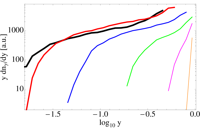
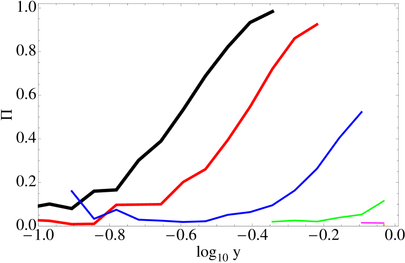
Figure 12: Intensity (left panel) and polarization degree (right panel) of the inverse Compton emission in the direction $(\theta_{\rm l},\phi_{\rm l})=$ $(85^{\circ},0)$ from monoenergetic isotropic electrons scattering monoenergetic unidirectional photons ($\epsilon=0.0025$, ${\bf\hat{k}}=$(0,0,1), ${\bf s}=(1,1,0)$). From left to right, the lines display the results for $\gamma$-values of 10, 100, 500, 2,500, 12,500, and 62,500. In the EF, the target photon energy in units of the electron mass is 0.02, 0.2, 1.1, 5.7, 29, 143 for the six simulated cases. In the right panel, the frequencies are given in units of the maximum kinematically allowed frequency $y=\omega_{\rm s}/\omega_{\rm max,KN}$, and the plotting ranges are restricted to the ranges where the statistical errors on the polarization degree are sufficiently small.

Figure 12 presents the intensity and polarization degree for a monoenergetic and unidirectional photon beam with an initial Stokes vector (1,1,0) scattering off monoenergetic isotropic electrons. We choose $\epsilon=1/400$ ($\sim$ 1.3 keV), ${\bf\hat{k}}$ $=(0,0,1)$, and an observer at ${\bf\hat{l}}$ $=(\cos{85^{\circ}},0,\sin{85^{\circ}})$. We simulate $\gamma$-values between 10 and 62,500 leading to $\epsilon^{\prime}$-values (computed with $\mu_{\rm kl}$ as proxi for $\mu_{\rm kp}$) between 0.02 and 143. All distributions are shown as function of the frequency $\omega_{\rm s}$ in units of the maximum frequency allowed kinematically

$$\omega_{\rm max,KN}=\frac{4\gamma^{2}\omega}{1+4\gamma\omega}.$$ (56)

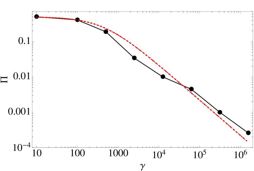
Figure 13: Net-polarization degree of all emitted photons as function of the electron Lorentz factor (solid line and circles) for the simulations of Figure 12 with additional simulations for $\gamma$-values of $3.125\times 10^{5}$ and $1.5625\times 10^{6}$. The dashed line displays the function $\Pi=0.5/(1+\epsilon^{\prime})$ showing that the net-polarization degree goes down approximately as the inverse of the EF target photon energy $\epsilon^{\prime}$.

Deeper into the Klein-Nishina regime (at larger $\epsilon^{\prime}$-values), the intensity distribution is more and more peaked towards $\omega_{\rm max,KN}$, and the polarization is strongly suppressed. Figure 13 displays the net-polarization degree as a function of $\gamma$. To guide the eye, the figure compares the numerical polarization degree results with the function $\Pi=0.5/(1+\epsilon^{\prime})$. The latter function agrees with the numerical results for scattering in the Thomson regime, but deviates considerably in the mild and deep Klein-Nishina regimes.

4 Discussion: Application to GEMS observations

In this paper, we describe a general formalism that can be used to study the polarization of inverse Compton emission, including SSC emission. The comparison of the numerical results with the analytical results of BCS and BS validate the analytical results for $\gamma$ $\stackrel{{\scriptstyle>}}{{\scriptstyle\sim}}$ 10. The numerical simulations show that Equations (49), (50), (55), and (38-39) can be used to predict the polarization properties of inverse Compton and SSC emission. An important qualitative result is that inverse Compton scattering of unpolarized target photons does not create a polarized signal as long as the electron distribution is isotropic over angular scales of $\gamma^{-1}$ and the electron Lorentz factors exceed minimum values of $\sim$10.

The GEMS X-ray polarimetry mission will have the opportunity to make major discoveries concerning AGNs, including constraints on the structure of accretion disk coronae (Schnittman & Krolik, 2010), the role and structure of the magnetic field in AGN jets, and the origin of the low-energy and high-energy components of the continuum emission from blazars (Krawczynski, 2011). Most relevant in the context of this paper are GEMS observations of the spatially unresolved continuum emission from blazar jets, because blazars are very bright X-ray sources. Two classes of objects are of particular interest. Flat spectrum radio quasars (FSRQs) and low frequency and intermediate frequency peaked BL Lac objects (LBLs and IBLs) with energy spectra with a $\nu F_{\nu}$-peak in the IR/optical/UV band and one in the MeV to GeV band, and high frequency peaked BL Lac objects (HBLs) with one $\nu F_{\nu}$-peak in the UV/X-ray band and one in the GeV/TeV band (see Abdo et al., 2010; Giommi et al., 2002, for compilations of spectral energy distributions).

In the case of HBLs (e.g. the X-ray bright sources Mrk 421, Mrk 501, 1ES1959+650, PKS 2155-314, and PKS 1218+304), GEMS will sample the low-energy emission component, presumably of synchrotron origin. Optical blazar observations exhibit rather high polarization degrees, often close to the theoretical maximum $\Pi_{\rm S}$ for synchrotron emission (e.g. Angel & Stockman, 1980; Scarpa & Falomo, 1997). If X-ray emission from HBLs is also synchrotron emission, a commonly made assumption, GEMS observations should reveal X-ray polarization degrees and directions similar to those observed in the optical band. Indeed, the polarization degrees could be even higher, as X-ray emitting electrons radiatively loose their energy on shorter time scales than optically emitting electrons. As the X-ray emitting electrons have thus less time to travel away from the acceleration sites, the X-ray bright regions are expected to be smaller than the optically bright regions. The more uniform magnetic field in the smaller X-ray bright regions should lead to a higher polarization degree of the synchrotron emission. The same reasoning suggests the possibility that continuous swings of the polarization direction as occasionally observed in the optical (e.g. Marscher et al., 2008), might be observed more often in the X-ray band. The polarization swings have been interpreted to arise from the movement of a helical magnetic field which threads the jet through stationary shocks (Marscher et al., 2008). Thus, GEMS has the potential to deliver observational evidence for a helical magnetic field at the bases of jets, a prediction of magnetic models of jet formation, acceleration, and collimation (e.g. Spruit, 2010, and references therein).

For FSRQs (e.g. the bright sources 3C 279, S 52116+81, and 1ES 0836+710), LBLs (e.g. the bright sources BL Lac, ON 231, and OJ 287), and some IBLs, GEMS will sample the high-energy $\nu F_{\nu}$-component, presumably of inverse Compton origin, and can be used to constrain the origin of this component. If the emission is of SSC origin, the inverse Compton emission should track the polarization degree and polarization direction of the synchrotron emission. Figures 9 and 10 show that the SSC emission can be highly polarized. In external-Compton (EC) models, the dominant target photons come from the accretion disk, from the corona, from the broad line region clouds (BLR), or the CMB. As discussed in Section 3.3, unpolarized target photons would result in very low ($\ll 1\%$) polarization degrees. Although reflection off the BLR clouds would polarize the target photons coming from a particular direction, averaging over an axisymmetric cloud configuration would lead to a low net-polarization of the target photons and thus to a rather low polarization degree of the EC emission. The detection of high polarization degrees would thus strongly favor a SSC origin of the X-ray emission. However, the detection of vanishing or low polarization degrees would not exclude the SSC scenario, as the SSC process can produce small polarization degrees if the magnetic field is aligned with the line of sight. The SSC hypothesis would even be consistent with low polarization degrees observed for many sources, as it cannot be excluded that the blazar-zone magnetic field is preferentially aligned with the line of sight. If the polarization degree is low but non-zero, simultaneous optical/X-ray measurements of the polarization degree and direction should be able to decide between an SSC and an EC origin, as the former predicts a good correlation while the latter does not.

In the discussion so far, we have assumed that the magnetic field, and the target photon and electron distributions do not change over the emission region. If information about the spatial (and/or temporal) distributions of these quantities is available, the polarization degree can be calculated with a calculation similar to Equation (55). In this case, one needs to integrate the expression in the nominator (inside the absolute-value brackets) and in the denominator over the emission volume. Inside the integrals, the magnetic field as well as the target photon and electron densities should be evaluated at the retarded times. As Equation (55) gives only $|q|/i$, one has to calculate also $|u|/i$ by replacing $\cos 2\chi$ in the nominator by $\sin 2\chi$. The polarization direction and degree can then be computed with Equations (3) and (4), respectively. In most cases, a spatial variation of the source properties will lead to a large number of free model parameters, and will render the unambiguous interpretation of observational data more difficult. Some of the most interesting GEMS results may come from observations of polarization degrees close to the maximum theoretically possible polarization degrees, which indicate a uniform emission region and make it possible to constrain models effectively. The reader interested in non-uniform emission regions should refer to the related discussions of the polarization of synchrotron emission from non-uniform emission regions (e.g. Begelman, 1993; Ruszkowski & Begelman, 2002, and references therein).

The Monte Carlo approach presented in Section 2 can also be used to explore the polarization properties of inverse Compton emission in the case that the electron phase space distribution is not isotropic in any frame of reference. Future research could combine the results of general relativistic or Newtonian magnetohydrodynamical simulations concerning the structure of blazar jets (see e.g. McKinney & Blandford, 2009; Meliani & Keppens, 2009, and references therein) with the results from particle-in-cell simulations of relativistic shocks (see e.g. Sironi & Spitkovsky, 2009, 2011, and references therein) to derive estimates of the electron phase space distribution. Monte Carlo simulations as described in this paper can then be used to derive observational signatures which can be compared to experimental data.

Figure 2: We define the polarization direction of a photon propagating along ${\bf\hat{k}}$ with reference to a right handed coordinate system $C=\{{\bf\hat{x}},{\bf\hat{y}},{\bf\hat{z}}\}$ with ${\bf\hat{z}}={\bf\hat{k}}$. The electric field vector of photons with a Stokes parameter $q/i=$1 is aligned with the $y$-axis, that of photons with $q/i=$-1 is aligned with $x$-axis. Looking along -${\bf\hat{k}}$, the directions with $u/i$=1 and $u/i$=-1 are rotated counterclockwise by $\pi/4$ relative to the $q/i=$1 and $q/i=$-1 directions, respectively. The polarization angle $\chi$ is measured clockwise from the direction with $q/i=$1.

Figure 11: Stokes $i$ parameter (left panel) and polarization degree $\Pi$ (right panel) of the inverse Compton emission from a monoenergetic unidirectional electron beam ($\gamma=2,500$, $(\theta_{\rm e},\phi_{\rm e})=$ $(85^{\circ},0)$) scattering a monoenergetic unidirectional photon beam ($\epsilon=0.01$, ${\bf\hat{k}}=$(0,0,1), ${\bf s}=(1,1,0)$) in the Klein-Nishina regime ($\epsilon^{\prime}=$22.8).

References

- Abdo et al. (2010) Abdo, A. A., et al. 2010, ApJ, 716, 30
- Angel & Stockman (1980) Angel, J. R. P., Stockman, H. S. 1980, ARA&A, 8, 321
- Begelman (1993) Begelman, M. C. 1993, Lect. Not.in Phys., 421, 145
- Begelman & Sikora (1987) Begelman, M. C., & Sikora, M. 1987, ApJ, 322, 650
- Bellazini et al. (2010) Bellazini, R., Costa, E., Matt, G., et al. 2010, ”X-ray Polarimetry: A New Window in Astrophysics”, Cambridge University Press.
- Bjornsson & Blumenthal (1982) Bjornsson, C.-I., & Blumenthal, G. R. 1982, ApJ, 259, 805
- Bjornsson (1985) Bjornsson, C.-I. 1985, MNRAS, 216, 241
- Black et al. (2010) Black, J. K., Deines-Jones, P., Hill, J. E., et al. 2010, ”The GEMS photoelectric x-ray polarimeters”, Space Telescopes and Instrumentation 2010: Ultraviolet to Gamma Ray. Edited by Arnaud, Monique; Murray, Stephen S.; Takahashi, Tadayuki. Proceedings of the SPIE, 7732, 77320X
- Blandford & Payne (1982) Blandford, R. D., Payne, D. G. 1982, MNRAS, 199, 883
- Bonometto, Cazzola, & Saggion (1970) Bonometto, S., Cazzola, P., & Saggion, A. (BCS) 1970, A&A, 7, 292
- Bonometto & Saggion (1973) Bonometto, S., & Saggion, A. (BS) 1973, A&A, 23, 9
- Celotti & Matt (1994) Celotti, A., & Matt, G. (CM) 1994, MNRAS, 268, 451
- De Young (1966) De Young, D. S. 1966, Journal of Mathematical Physics, 7, 1916
- Dean et al. (2008) Dean, A. J., Clark, D. J., Stephen, J. B., et al. 2008, Science, 321, 1183
- Depaola (2003) Depaola, G. O. 2003, NIMA, 512, 619
- Dolan (1967) Dolan, J. F. 1967, Space Sci. Rev., 6, 579
- Fano (1949) Fano, U. 1949, J. Opt. Soc. Am. 39, 859
- Fano (1957) Fano, U. 1957, Revs. Modern Phys. 29, 74
- Forot et al. (2008) Forot, M., Laurent, P., Grenier, I. A., et al. 2008, ApJ, 688, L29
- Ginzburg & Syrovatskii (1965) Ginzburg, V. L., Syrovatskii, S. I. 1965, ARA&A, 3, 297
- Giommi et al. (2002) Giommi,P.,Capalbi,M.,Fiocchi,M., Memola, E., Perri, M., Piranomonte, S., Rebecchi, S., Massaro, E. 2002, “A Catalog of 157 X-ray Spectra and 84 Spectral Energy Distributions of Blazars observed with BeppoSAX”, Procs.: “Blazar Astrophysics with BeppoSAX and other Observatories” (Frascati, December 2001), eds. Paolo Giommi, Enrico Massaro and Giorgio Palumbo [arXiv:astro-ph0209596], http: www.asdc.asi.itblazars
- Kaaret et al. (2009) Kaaret, P., Swank, J., Jahoda, K., et al. 2009, ”The Gravity and Extreme Magnetism Small Explorer (GEMS)”, Publication: Chandra’s First Decade of Discovery, Proceedings of the conference held 22-25 September, 2009 in Boston, MA. Edited by Scott Wolk, Antonella Fruscione, and Douglas Swartz, abstract #125
- Krawczynski (2011) Krawczynski, H. 2011, Astroparticle Physics, 34, 784
- Krawczynski (2011) Krawczynski, H., Garson, A., Guo, Q., Baring, M. G., Ghosh, P., Beilicke, M., & Lee, K. 2011, Astroparticle Physics, 34, 550
- Laing (1980) Laing, R. A., 1980, MNRAS, 193, 439
- Laurent et al. (2011) Laurent, P., Rodriguez, J., Wilms, J., Cadolle Bel, M., Pottschmidt, K., Grinberg, V. 2011, Science Express, Science DOI: 10.1126/science.1200848
- Lei, Dean, Hills et al. (1997) Lei, F., Dean, A. J., Hills, G. L. 1997, Space Sci. Rev., 82, 309
- Lightman & Shapiro (1975) Lightman, A. P., Shapiro, S. L. 1975, ApJ, 198, L73
- Lightman & Shapiro (1976) Lightman, A. P., Shapiro, S. L. 1976, ApJ, 203, 701
- Marscher et al. (2008) Marscher, A. P., et al. 2008, Nature, 452, 966
- Matt et al. (1996) Matt, G., Feroci, M., Rapisarda, M., & Costa, E. 1996, Radiation Physics and Chemistry, 48, 403
- McKinney & Blandford (2009) McKinney, J. C., & Blandford, R. D. 2009, MNRAS, 394, L126
- McMaster (1961) McMaster, W. H. 1961, Reviews of Modern Physics, 33, 8
- McNamara et al. (2008) McNamara, A. L., Kuncic, Z., & Wu, K. 2008, MNRAS, 386, 2167
- McNamara et al. (2009) McNamara, A. L., Kuncic, Z., & Wu, K. 2009, MNRAS, 395, 1507
- Meliani & Keppens (2009) Meliani, Z. and Keppens, R. 2009, ApJ, 705, 1594
- Meszaros et al. (1988) Meszaros, P., Novick, R., Szentgyorgyi, A., et al. 1988, ApJ, 324, 1056
- Nagirner & Poutanen (1993) Nagirner, D. I., & Poutanen, J. 1993, A&A, 275, 325
- Novick et al. (1977) Novick, R., Kestenbaum, H. L., Long, K. S., et al. 1977, ”OSO-8 X-ray polarimeter and Bragg crystal spectrometer observations”, In: Highlights of astronomy. Volume 4 - International Astronomical Union, General Assembly, 16th, Grenoble, France, August 24-September 2, 1976, Proceedings. Part 1. (A78-16417 04-88) Dordrecht, D. Reidel Publishing Co., 1977, 95
- Poutanen (1994) Poutanen, J. 1994, ApJS, 92, 607
- Rees (1975) Rees, M. J. 1975, MNRAS, 171, 457
- Rybicki & Lightman (1986) Rybicki, G. B., Lightman, A. P. 1986, “Radiative Processes in Astrophysics”, Wiley-VCH
- Ruszkowski & Begelman (2002) Ruszkowski, M., & Begelman, M. C. 2002, ApJ, 573, 485
- Scarpa & Falomo (1997) Scarpa, R., Falomo, R. 1997, A&A, 325, 109
- Schnittman & Krolik (2010) Schnittman, J. D., Krolik, J. H. 2010, ApJ, 712, 908
- Sironi & Spitkovsky (2009) Sironi, L., & Spitkovsky, A. 2009, ApJ, 698, 1523
- Sironi & Spitkovsky (2011) Sironi, L., & Spitkovsky, A. 2011, ApJ, 726, 75
- Spruit (2010) Spruit, H. C. 2010, “Lecture Notes in Physics”, Berlin Springer Verlag, 794, 233
- Vlahakis & Königl (2004) Vlahakis, N., Königl, A. 2004, ApJ, 605, 656
- Weisskopf et al. (1978) Weisskopf, M. C., Silver, E. H., Kestenbaum, H. L., et al. 1978, ApJ, 220, L117
- Weisskopf et al. (2006) Weisskopf, M. C., Elsner, R. F., Hanna, D., et al. 2006, ”The prospects for X-ray polarimetry and its potential use for understanding neutron stars”, Paper presented at the 363rd Heraeus Seminar in Bad Honnef, Germany, [arXiv:astro-ph/0611483]