Numerical Optimization of Eigenvalues of Hermitian Matrix Functions

Abstract

This work concerns the global minimization of a prescribed eigenvalue or a weighted sum of prescribed eigenvalues of a Hermitian matrix-valued function depending on its parameters analytically in a box. We describe how the analytical properties of eigenvalue functions can be put into use to derive piece-wise quadratic functions that underestimate the eigenvalue functions. These piece-wise quadratic under-estimators lead us to a global minimization algorithm, originally due to Breiman and Cutler. We prove the global convergence of the algorithm, and show that it can be effectively used for the minimization of extreme eigenvalues, e.g., the largest eigenvalue or the sum of the largest specified number of eigenvalues. This is particularly facilitated by the analytical formulas for the first derivatives of eigenvalues, as well as analytical lower bounds on the second derivatives that can be deduced for extreme eigenvalue functions. The applications that we have in mind also include the ${\rm H}_{\infty}$-norm of a linear dynamical system, numerical radius, distance to uncontrollability and various other non-convex eigenvalue optimization problems, for which, generically, the eigenvalue function involved is simple at all points.

Key words. Hermitian eigenvalues, analytic, global optimization, perturbation of eigenvalues, quadratic programming

AMS subject classifications. 65F15, 90C26

1 Introduction

The main object of this work is a matrix-valued function ${\mathcal{A}}(\omega):{\mathbb{R}}^{d}\rightarrow{\mathbb{C}}^{n\times n}$ that is analytic and Hermitian at all $\omega\in{\mathbb{R}}^{d}$. Here, we consider the numerical global minimization of a prescribed eigenvalue $\lambda(\omega)$ of ${\mathcal{A}}(\omega)$ over $\omega\in{\mathcal{B}}\subseteq{\mathbb{R}}^{d}$, where ${\mathcal{B}}$ denotes a box. From an application point of view, a prescribed eigenvalue typically refers to the $j$th largest eigenvalue, i.e., $\lambda(\omega):=\lambda_{j}({\mathcal{A}}(\omega))$, or a weighted sum of $j$ largest eigenvalues, i.e., $\lambda(\omega):=\sum_{k=1}^{j}d_{k}\lambda_{k}({\mathcal{A}}(\omega))$ for given real numbers $d_{1},\dots,d_{j}$. However, it may as well refer to a particular eigenvalue with respect to a different criterion as long as the (piece-wise) analyticity properties discussed below and in Section 3 are satisfied.

The literature from various engineering fields and applied sciences is rich with eigenvalue optimization problems that fits into the setting of the previous paragraph. There are problems arising in structural design and vibroacoustics, for which the minimization of the largest eigenvalue or maximization of the smallest eigenvalue of a matrix-valued function is essential, e.g., the problem of designing the strongest column which originated from Euler in the 18th century [30]. In control theory, various quantities regarding dynamical systems can be posed as eigenvalue optimization problems. For instance, the distance from a linear dynamical system to a nearest unstable system [47], and the ${\rm H}_{\infty}$-norm of a linear dynamical system have non-convex eigenvalue optimization characterizations [3]. In graph theory, relaxations of some NP-hard graph partitioning problems give rise to optimization problems in which the sum of the $j$ largest eigenvalues is to be minimized [10].

In this paper, we offer a generic algorithm based on the analytical properties of eigenvalues of an analytic and Hermitian matrix-valued function, that is applicable for any eigenvalue optimization problem whenever lower bounds on the second derivatives of the eigenvalue function can be calculated analytically or numerically. All of the existing global eigenvalue optimization algorithms in the non-convex setting are designed for specific problems, e.g., [3, 5, 6, 7, 15, 17, 19, 20, 21, 22, 32], while widely adopted techniques such as interior point methods [34] - when it is possible to pose an eigenvalue optimization problem as a semi-definite program - or a bundle method [31] are effective in the convex setting. We foresee non-convex eigenvalue optimization problems that depend on a few parameters as the typical setting for the use of the algorithm here.

For the optimization of non-convex eigenvalue functions, it appears essential to benefit from the global properties of eigenvalue functions, such as their global Lipschitzness or global bounds on their derivatives. Such global properties lead us to approximate $\lambda(\omega)$ globally with under-estimating functions, which we call support functions. Furthermore, the derivatives of the eigenvalue functions can be evaluated effectively at no cost once the eigenvalue function is evaluated (due to analytic expressions for the derivatives of eigenvalues in terms of eigenvectors as discussed in Section 3.2.1). Therefore, the incorporation of the derivatives into the support functions yields quadratic support functions on which our algorithm relies. The quadratic support functions for eigenvalue functions are derived exploiting the analytical properties of eigenvalues and presume the availability of a lower bound $\gamma$ on the second derivatives of the eigenvalue function that is obtained either analytically or numerically.

Example: Consider the minimization of the largest eigenvalue $\lambda_{1}(\omega)=\lambda_{1}\left({\mathcal{A}}(\omega)\right)$ of

$${\mathcal{A}}:{\mathbb{R}}\rightarrow{\mathbb{R}}^{n\times n},\;\;\;{\mathcal{A}}(\omega):=A_{0}+\omega A_{1}+\omega^{2}A_{2},$$

where $A_{0},A_{1},A_{2}\in{\mathbb{R}}^{n\times n}$ are given symmetric matrices. It can be deduced from the expressions in Section 3.2.2 that $\lambda_{1}^{\prime\prime}(\omega)\geq\gamma:=2\lambda_{\min}\left(A_{2}\right)$ for all $\omega$ such that $\lambda_{1}(\omega)$ is simple. Furthermore, due to expressions in Section 3.2.1, at all such $\omega$, we have $\lambda_{1}^{\prime}(\omega)=v_{1}(\omega)^{T}(A_{1}+2\omega A_{2})\;v_{1}(\omega),$ where $v_{1}(\omega)$ is a unit eigenvector associated with $\lambda_{1}(\omega)$. Consequently, it turns out that, about any $\omega_{k}\in{\mathbb{R}}$ where $\lambda_{1}(\omega_{k})$ is simple, there is a support function

$$q(\omega):=\lambda_{1}(\omega_{k})+\lambda_{1}^{\prime}(\omega_{k})(\omega-\omega_{k})+\frac{\gamma}{2}(\omega-\omega_{k})^{2}$$

satisfying $q(\omega)\leq\lambda_{1}(\omega)$ for all $\omega\in{\mathbb{R}}$; see Section 5.2 for the details.

Support functions have earlier been explored by the global optimization community. The Piyavskii-Shubert algorithm [40, 45] is derivative-free, and constructs conic support functions based on Lipschitz continuity with a known global Lipschitz constant. It converges sub-linearly in practice. Sophisticated variants that make use of several Lipschitz constants simultaneously appeared in the literature [24, 43]. The idea of using derivatives in the context of global optimization yields powerful algorithms. Breimann and Cutler [4] developed an algorithm that utilizes quadratic support functions depending on the derivatives. Some variants of the Breimann-Cutler algorithm are also suggested for functions with Lipschitz-continuous derivatives; for instance [18, 26, 27] benefit from multiple Lipschitz constants for the derivatives, [42] estimates Lipschitz constants for the derivatives locally, while [29] modifies the support functions of the Breimann-Cutler algorithm in the univariate case so that the subproblems become smooth; however, all these variants in the multivariate case end up working on a mesh as a downside. The quadratic support functions that we derive for $\lambda(\omega)$ coincide with the quadratic support functions on which the Breimann-Cutler algorithm is built on. Consequently, our approach is a variant of the algorithm due to Breimann and Cutler [4].

At every iteration of the algorithm, a global minimizer of a piece-wise quadratic model defined as the maximum of a set of quadratic support functions is determined. A new quadratic support function is constructed around this global minimizer, and the piece-wise quadratic model is refined with the addition of this new support function. In practice, we observe a linear rate of convergence to a global minimizer.

The algorithm appears applicable especially to extremal eigenvalue functions of the form

$$\lambda(\omega)=\sum_{k=1}^{j}d_{k}\lambda_{k}\left({\mathcal{A}}(\omega)\right),$$

where $d_{k}$ are given real numbers such that $d_{1}\geq d_{2}\geq\dots\geq d_{j}\geq 0$. This is facilitated by the simple quadratic support functions derived in Section 5.2, and expressions for the lower bound $\gamma$ on the second derivatives derived in Section 6. The algorithm is also applicable if the eigenvalue function $\lambda(\omega)$ is simple over all $\omega\in{\mathcal{B}}$, which holds for various eigenvalue optimization problems of interest.

Outline: We start in the next section with a list of eigenvalue optimization problems to which our proposed algorithm fits well. In Section 3, the basic results concerning the analyticity and derivatives of the eigenvalues of a Hermitian matrix-valued function ${\mathcal{A}}(\omega)$ that depends analytically on $\omega$ are reviewed. In Section 4, for a general eigenvalue function, the piece-wise quadratic support functions that are defined as the minimum of $n$ quadratic functions are derived. In Section 5, it is shown that these piece-wise quadratic support functions simplify to smooth quadratic support functions for the extremal eigenvalue functions, as well as for the eigenvalue functions that are simple for all $\omega\in{\mathcal{B}}$. Global lower bounds $\gamma$ on the second derivatives of an extremal eigenvalue function are deduced in Section 6. The algorithm based on the quadratic support functions is presented in Section 7. We establish the global convergence of the proposed algorithm in Section 8. Finally, comprehensive numerical experiments are provided in Section 9. The examples indicate the superiority of the algorithm over the Lipschitz continuity based algorithms, e.g., [24, 40, 45], as well as the level-set based approaches devised for particular non-convex eigenvalue optimization problems, e.g., [20, 32]. The reader who prefers to avoid technicalities at first could glance at the algorithm in Section 7, then go through Sections 3-6 for the theoretical foundation.

2 Applications

2.1 Quantities Related to Dynamical Systems

The numerical radius $r(A)$ of $A\in{\mathbb{C}}^{n\times n}$ is the modulus of the outer-most point in its field of values [23], and is defined by

$$r(A):=\max\{|z^{\ast}Az|\;|\;z\in{\mathbb{C}}^{n}\;\;{\rm s.t.}\;\;\|z\|_{2}=1\}.$$

This quantity gives information about the powers of $A$, e.g.,$\|A^{k}\|\leq 2r(A)^{k}$, and is used in the literature to analyze the convergence of iterative methods for the solution of linear systems [1, 11]. An eigenvalue optimization characterization is given by [23]:

$$r(A)=-\left[\min_{\theta\in[0,2\pi]}\;\lambda_{n}\left({\mathcal{A}}(\theta)\right)\right],\;\;\;\;{\mathcal{A}}(\theta):=-(Ae^{i\theta}+A^{\ast}e^{-i\theta})/2.$$

The ${\rm H}_{\infty}$-norm is one of the most widely used norms in practice for the descriptor system

$$Ex^{\prime}(t)=Ax(t)+Bu(t),\;\;{\rm and}\;\;y(t)=Cx(t)+Du(t),$$

where $u(t)$ and $y(t)$ are the input and output functions, respectively, and $E,A\in{\mathbb{C}}^{n\times n}$, $B\in{\mathbb{C}}^{n\times m},C\in{\mathbb{C}}^{p\times n},D\in{\mathbb{C}}^{p\times m}$ with $m,p\leq n$ are the system matrices. The ${\rm H}_{\infty}$-norm of the transfer function for this system is defined as

$$\|H\|_{\infty}:=\frac{1}{\inf_{\omega\in{\mathbb{R}}}\;\sigma_{n}\left[H(i\omega)^{\dagger}\right]},\;\;\;\;H(s):=\left[C(sE-A)^{-1}B+D\right].$$

Here and elsewhere, $\sigma_{j}(\cdot)$ represents the $j$th largest singular value, and $H(i\omega)^{\dagger}$ denotes the pseudoinverse of $H(i\omega)$. Also above, with zero initial conditions for the descriptor system, the transfer function $H(s)$ reveals the linear relation between the input and output, as $Y(s)=H(s)U(s),$ with $U(s)$ and $Y(s)$ denoting the Laplace transformations of $u(t)$ and $y(t)$, respectively. Note that the ${\rm H}_{\infty}$-norm above is ill-posed (i.e., the associated operator is unbounded) if the pencil $L(\lambda)=A-\lambda E$ has an eigenvalue on the imaginary axis or to the right of the imaginary axis. Therefore, when the ${\rm H}_{\infty}$-norm is well-posed, the matrix-valued function ${\mathcal{A}}(\omega):=H(i\omega)$ is analytic at all $\omega\in{\mathbb{R}}$. A relevant quantity is the (continuous) distance to instability from a matrix $A\in{\mathbb{C}}^{n\times n}$; the eigenvalue optimization characterization for the ${\rm H}_{\infty}$-norm with $E=B=C=I_{n}$ and $D=0$ reduces to that for the distance to instability [47] from $A$ with respect to the $\ell_{2}$-norm.

Paige [39] suggested the distance to uncontrollability, for a given $A\in{\mathbb{C}}^{n\times n}$ and $B\in{\mathbb{C}}^{n\times m}$ with $m\leq n$, defined by

$$\tau(A,B):=\inf\left\{\left\|\left[\begin{array}[]{cc}\Delta A&\Delta B\end{array}\right]\right\|_{2}\;|\;(A+\Delta A,B+\Delta B)\;\;{\rm is}\;\;{\rm uncontrollable}\right\},$$

as a robust measure of controllability. Here, the controllability of a linear control system $(A,B)$ of the form $x^{\prime}(t)=Ax(t)+Bu(t)$ means that the function $x(t)$ can be driven into any state at a particular time by some input $u(t)$, and could be equivalently characterized as ${\rm rank}\left(\left[\begin{array}[]{cc}A-zI&B\end{array}\right]\right)=n,\;\;\;\forall z\in{\mathbb{C}}.$ Therefore, the eigenvalue optimization characterization for the distance to uncontrollability takes the form [12]:

$$\tau(A,B)=\min_{z\in{\mathbb{C}}}\sigma_{n}\left({\mathcal{A}}(z)\right),\;\;\;\;{\mathcal{A}}(z):=\left[\begin{array}[]{cc}A-zI&B\end{array}\right].$$

2.2 Minimizing the Largest or Maximizing the Smallest Eigenvalues

In the 18th century, Euler considered the design of the strongest column with a given volume with respect to the radii of the cross-sections [30, 37]. The problem can be formulated as finding the parameters, representing the radii of cross-sections, maximizing the smallest eigenvalue of a fourth order differential operator. The analytical solution of the problem has been considered in several studies in 1970s and in 1980s [2, 33, 35], which were motivated by the earlier work of Keller and Tadjbakhsh [46]. Later, the problem is treated numerically [8] by means of the finite-element discretization, giving rise to the problem

$${\rm min}_{\omega\in{\mathbb{R}}^{d}}\;\lambda_{1}\left({\mathcal{A}}(\omega)\right).$$ (1)

The treatment in [8] yields ${\mathcal{A}}(\omega):=A_{0}+\sum_{j=1}^{d}\omega_{j}A_{j}$. In this affine setting, the minimization of the largest eigenvalue is a convex optimization problem (immediate from Theorem 6 below) and received considerable attention [14, 16, 36].

In the general setting, when the dependence of the matrix function ${\mathcal{A}}(\omega)$ on the parameters is not affine, the problem in (1) is non-convex. Such non-convex problems are significant (though they are not studied much excluding a few studies such as [38] that offer only local analysis) in robust control theory for instance to ensure robust stability. The dual form that concerns the maximization of the smallest eigenvalue is of interest in vibroacoustics.

2.3 Minimizing the Sum of the $j$ Largest Eigenvalues

In graph theory, relaxations of the NP-hard partitioning problems lead to eigenvalue optimization problems that require the minimization of the sum of the $j$ largest eigenvalues. For instance, given a weighted graph with $n$ vertices and nonnegative integers $d_{1}\geq d_{2}\geq\dots\geq d_{j}$ summing up to $n$, consider finding a partitioning of the graph such that the $\ell$th partition contains exactly $d_{\ell}$ vertices for $\ell=1,\dots,j$ and the sum of the weights of the edges within each partition is maximized. The relaxation of this problem suggested in [10] is of the form

$${\rm min}_{\omega\in{\mathbb{R}}^{d}}\;\sum_{k=1}^{j}d_{k}\lambda_{k}\left({\mathcal{A}}(\omega)\right).$$ (2)

The problem (2) is convex, if ${\mathcal{A}}(\omega)$ is an affine function of $\omega$, as in the case considered by [10], see also [9].

Once again, in general, the minimization of the sum of the $j$ largest eigenvalues is not a convex optimization problem, and there are a few studies in the literature that attempted to analyze the problem locally for instance around the points where the eigenvalues coalesce [44].

3 Background on Perturbation Theory of Eigenvalues

In this section, we first briefly summarize the analyticity results, mostly borrowed from [41, Chapter 1], related to the eigenvalues of matrix-valued functions. Then, expressions [28] are provided for the derivatives of Hermitian eigenvalues in terms of eigenvectors and the derivatives of matrix-valued functions. Finally, we elaborate on the analyticity of singular value problems as special Hermitian eigenvalue problems.

3.1 Analyticity of Eigenvalues

3.1.1 Univariate Matrix Functions

For a univariate matrix-valued function ${\mathcal{A}}(\omega)$ that depends on $\omega$ analytically, which may or may not be Hermitian, the characteristic polynomial is of the form

$$g(\omega,\lambda):=\det(\lambda I-{\mathcal{A}}(\omega))=a_{n}(\omega)\lambda^{n}+\dots+a_{1}(\omega)\lambda+a_{0}(\omega),$$

where $a_{0}(\omega),\dots,a_{n}(\omega)$ are analytic functions of $\omega$. It follows from the Puiseux’ theorem (see, e.g., [48, Chapter 2]) that each root $\tilde{\lambda}_{j}(\omega)$ such that $g(\omega,\tilde{\lambda}_{j}(\omega))=0$ has a Puiseux series of the form

$$\tilde{\lambda}_{j}(\omega)=\sum_{k=0}^{\infty}c_{k,j}\omega^{k/r},$$ (3)

for all small $\omega$, where $r$ is the multiplicity of the root $\tilde{\lambda}_{j}(0)$.

Now suppose ${\mathcal{A}}(\omega)$ is Hermitian for all $\omega$, and let $\ell$ be the smallest integer such that $c_{\ell,j}\neq 0$. Then, we have

$$\lim_{\omega\rightarrow 0^{+}}\frac{\tilde{\lambda}_{j}(\omega)-\tilde{\lambda}_{j}(0)}{\omega^{\ell/r}}=c_{\ell,j},$$

which implies that $c_{\ell,j}$ is real, since $\tilde{\lambda}_{j}(\omega)$ and $\omega^{\ell/r}$ are real numbers for each $\omega$. Furthermore,

$$\lim_{\omega\rightarrow 0^{-}}\frac{\tilde{\lambda}_{j}(\omega)-\tilde{\lambda}_{j}(0)}{(-\omega)^{\ell/r}}=(-1)^{\ell/r}c_{\ell,j}$$

is real, which implies that $(-1)^{\ell/r}$ is real, or equivalently that $\ell/r$ is integer. This observation reveals that the first nonzero term in the Puiseux series of $\tilde{\lambda}_{j}(\omega)$ is an integer power of $\omega$. The same argument applied to the derivatives of $\tilde{\lambda}_{j}(\omega)$ and the associated Puiseux series indicates that only integer powers of $\omega$ can appear in the Puiseux series (3), that is the Puiseux series reduces to a power series. This establishes that $\tilde{\lambda}_{j}(\omega)$ is an analytic function of $\omega$. Indeed, it can also be deduced that, associated with $\tilde{\lambda}_{1}(\omega),\dots,\tilde{\lambda}_{n}(\omega)$, there is an orthonormal set $\{v_{1}(\omega),\dots,v_{n}(\omega)\}$ of eigenvectors, where each of $v_{1}(\omega),\dots,v_{n}(\omega)$ varies analytically with respect to $\omega$ (see [41] for details).

Theorem 1 (Rellich).

Let ${\mathcal{A}}(\omega):{\mathbb{R}}\rightarrow{\mathbb{C}}^{n\times n}$ be a Hermitian matrix-valued function that depends on $\omega$ analytically.

• The $n$ roots of the characteristic polynomial of ${\mathcal{A}}(\omega)$ can be arranged so that each root $\tilde{\lambda}_{j}(\omega)$ for $j=1,\dots,n$ is an analytic function of $\omega$.

• There exists an eigenvector $v_{j}(\omega)$ associated with $\tilde{\lambda}_{j}(\omega)$ for $j=1,\dots,n$ that satisfies the following:

  1. $\left(\tilde{\lambda}_{j}(\omega)I-{\mathcal{A}}(\omega)\right)v_{j}(\omega)=0,\;\;\forall\omega\in{\mathbb{R}}$,

  2. $\|v_{j}(\omega)\|_{2}=1,\;\;\forall\omega\in{\mathbb{R}}$,

  3. $v_{j}^{\ast}(\omega)v_{k}(\omega)=0,\;\;\forall\omega\in{\mathbb{R}}$ for $k\neq j$, and

  4. $v_{j}(\omega)$ is an analytic function of $\omega$.

3.1.2 Multivariate Matrix Functions

The eigenvalues of a multivariate matrix-valued function ${\mathcal{A}}(\omega):{\mathbb{R}}^{d}\rightarrow{\mathbb{C}}^{n\times n}$ that depends on $\omega$ analytically do not have a power series representation in general even when ${\mathcal{A}}(\omega)$ is Hermitian. As an example, consider

$${\mathcal{A}}(\omega)=\left[\begin{array}[]{cc}\omega_{1}&\frac{\omega_{1}+\omega_{2}}{2}\\ \frac{\omega_{1}+\omega_{2}}{2}&\omega_{2}\\ \end{array}\right]\;\;\;{\rm with}\;\;\;\tilde{\lambda}_{1,2}(\omega)=\frac{\omega_{1}+\omega_{2}}{2}\pm\sqrt{\frac{\omega_{1}^{2}+\omega_{2}^{2}}{2}}.$$

On the other hand, it follows from Theorem 1 that, there are underlying eigenvalue functions $\tilde{\lambda}_{j}(\omega),\;j=1,\dots,n$, of ${\mathcal{A}}(\omega)$, each of which is analytic along every line in ${\mathbb{R}}^{d}$, when ${\mathcal{A}}(\omega)$ is Hermitian. This analyticity property along lines in ${\mathbb{R}}^{d}$ implies the existence of the first partial derivatives of $\tilde{\lambda}_{j}(\omega)$ everywhere. Expressions for the first partial derivatives will be derived in the next subsection, indicating their continuity. As a consequence of the continuity of the first partial derivatives, each $\tilde{\lambda}_{j}(\omega)$ must be differentiable.

Theorem 2.

Let ${\mathcal{A}}(\omega):{\mathbb{R}}^{d}\rightarrow{\mathbb{C}}^{n\times n}$ be a Hermitian matrix-valued function that depends on $\omega$ analytically. Then, the $n$ roots of the characteristic polynomial of ${\mathcal{A}}(\omega)$ can be arranged so that each root $\tilde{\lambda}_{j}(\omega)$ is (i) analytic on every line in ${\mathbb{R}}^{d}$, and (ii) differentiable on ${\mathbb{R}}^{d}$.

3.2 Derivatives of Eigenvalues

3.2.1 First Derivatives of Eigenvalues

Consider a univariate Hermitian matrix-valued function ${\mathcal{A}}(\omega)$ that depends on $\omega$ analytically. An analytic eigenvalue $\tilde{\lambda}_{j}(\omega)$ and the associated eigenvector $v_{j}(\omega)$ as described in Theorem 1 satisfy

$${\mathcal{A}}(\omega)v_{j}(\omega)=\tilde{\lambda}_{j}(\omega)v_{j}(\omega).$$

Taking the derivatives of both sides, we obtain

$$\frac{d{\mathcal{A}}(\omega)}{d\omega}v_{j}(\omega)+{\mathcal{A}}(\omega)\frac{dv_{j}(\omega)}{d\omega}=\frac{d\tilde{\lambda}_{j}(\omega)}{d\omega}v_{j}(\omega)+\tilde{\lambda}_{j}(\omega)\frac{dv_{j}(\omega)}{d\omega}.$$ (4)

Multiplying both sides by $v_{j}(\omega)^{\ast}$ and using the identities $v_{j}(\omega)^{\ast}{\mathcal{A}}(\omega)=v_{j}(\omega)^{\ast}\tilde{\lambda}_{j}(\omega)$ as well as $v_{j}(\omega)^{\ast}v_{j}(\omega)=\|v_{j}(\omega)\|^{2}_{2}=1$, we get

$$\frac{d\tilde{\lambda}_{j}(\omega)}{d\omega}=v_{j}(\omega)^{\ast}\frac{d{\mathcal{A}}(\omega)}{d\omega}v_{j}(\omega).$$ (5)

3.2.2 Second Derivatives of Eigenvalues

By differentiating both sides of (5), it is possible to deduce the formula (the details are omitted for brevity)

$$\frac{d^{2}\tilde{\lambda}_{j}(\omega)}{d\omega^{2}}=v_{j}(\omega)^{\ast}\frac{d^{2}{\mathcal{A}}(\omega)}{d\omega^{2}}v_{j}(\omega)+2\sum_{k=1,k\neq j}^{n}\frac{1}{\tilde{\lambda}_{j}(\omega)-\tilde{\lambda}_{k}(\omega)}\left|v_{k}(\omega)^{\ast}\frac{d{\mathcal{A}}(\omega)}{d\omega}v_{j}(\omega)\right|^{2}$$ (6)

for the second derivatives assuming that the (algebraic) multiplicity of $\tilde{\lambda}_{j}(\omega)$ is one.

If, on the other hand, the eigenvalues repeat at a given $\hat{\omega}$, specifically when the (algebraic) multiplicity of $\tilde{\lambda}_{j}(\hat{\omega})$ is greater than one, the formula (6) generalizes as

$$\frac{d^{2}\tilde{\lambda}_{j}(\hat{\omega})}{d\omega^{2}}=v_{j}(\hat{\omega})^{\ast}\frac{d^{2}{\mathcal{A}}(\hat{\omega})}{d\omega^{2}}v_{j}(\hat{\omega})+2\sum_{k=1,k\neq j,k\notin\alpha}^{n}\lim_{\tilde{\omega}\rightarrow\hat{\omega}}\left(\frac{1}{\tilde{\lambda}_{j}(\tilde{\omega})-\tilde{\lambda}_{k}(\tilde{\omega})}\left|v_{k}(\tilde{\omega})^{\ast}\frac{d{\mathcal{A}}(\tilde{\omega})}{d\omega}v_{j}(\tilde{\omega})\right|^{2}\right).$$ (7)

Here, $\alpha$ denotes the set of indices of the analytic eigenvalues (specified in Theorem 1) that are identical to $\tilde{\lambda}_{j}(\omega)$ at all $\omega$.

3.2.3 Derivatives of Eigenvalues for Multivariate Hermitian Matrix Functions

Let ${\mathcal{A}}(\omega):{\mathbb{R}}^{d}\rightarrow{\mathbb{C}}^{n\times n}$ be Hermitian and analytic. It follows from (5) that

$$\frac{\partial\tilde{\lambda}_{j}(\omega)}{\partial\omega_{k}}=v_{j}^{\ast}(\omega)\frac{\partial{\mathcal{A}}(\omega)}{\partial\omega_{k}}v_{j}(\omega).$$ (8)

Since ${\mathcal{A}}(\omega)$ and $v_{j}(\omega)$ are analytic with respect to $\omega_{\ell}$ for $\ell=1,\dots,n$, this implies the continuity, also the analyticity with respect to $\omega_{\ell}$, of each partial derivative $\partial\tilde{\lambda}_{j}(\omega)/\partial\omega_{k}$, and hence the existence of $\partial^{2}\tilde{\lambda}_{j}(\omega)/(\partial\omega_{k}\partial\omega_{\ell})$, everywhere. If the multiplicity of $\tilde{\lambda}_{j}(\omega)$ is one, differentiating both sides of (8) with respect to $\omega_{\ell}$ would yield the following expressions for the second partial derivatives.

$$\frac{\partial^{2}\tilde{\lambda}_{j}(\omega)}{\partial\omega_{k}\;\partial\omega_{\ell}}= v_{j}^{\ast}(\omega)\frac{\partial^{2}{\mathcal{A}}(\omega)}{\partial\omega_{k}\;\partial\omega_{l}}v_{j}(\omega)+\hskip 224.74911pt$$

$$2\cdot\Re\left(\sum_{m=1,m\neq j}^{n}\frac{1}{\tilde{\lambda}_{j}(\omega)-\tilde{\lambda}_{m}(\omega)}\left(v_{j}(\omega)^{\ast}\frac{\partial{\mathcal{A}}(\omega)}{\partial\omega_{k}}v_{m}(\omega)\right)\left(v_{m}(\omega)^{\ast}\frac{\partial{\mathcal{A}}(\omega)}{\partial\omega_{\ell}}v_{j}(\omega)\right)\right).$$

Expressions similar to (7) can be obtained for the second partial derivatives when $\tilde{\lambda}_{j}(\omega)$ has multiplicity greater than one.

3.3 Analyticity of Singular Values

Some of the applications (see Section 2.1) concern the optimization of the $j$th largest singular value of an analytic matrix-valued function. The singular value problems are special Hermitian eigenvalue problems. In particular, denoting the $j$th largest singular value of an analytic matrix-valued function ${\mathcal{B}}(\omega):{\mathbb{R}}^{d}\rightarrow{\mathbb{C}}^{n\times m}$ (not necessarily Hermitian) by $\sigma_{j}(\omega)$, the set of eigenvalues of the Hermitian matrix-valued function

$${\mathcal{A}}(\omega):=\left[\begin{array}[]{cc}0&{\mathcal{B}}(\omega)\\ {\mathcal{B}}(\omega)^{\ast}&0\\ \end{array}\right],$$

is $\{\sigma_{j}(\omega),-\sigma_{j}(\omega):j=1,\dots,n\}$. In the univariate case $\sigma_{j}(\omega)$ is the $j$th largest of the $2n$ analytic eigenvalues, $\tilde{\lambda}_{1}(\omega),\dots,\tilde{\lambda}_{2n}(\omega)$, of ${\mathcal{A}}(\omega)$. The multivariate $d$-dimensional case is similar, with the exception that each eigenvalue $\tilde{\lambda}_{j}(\omega)$ is differentiable and analytic along every line in ${\mathbb{R}}^{d}$. Let us focus on the univariate case throughout the rest of this section. Extensions to the multi-variate case are similar to the previous sections. Suppose $v_{j}(\omega):=\left[\begin{array}[]{c}u_{j}(\omega)\\ w_{j}(\omega)\end{array}\right]$, with $u_{j}(\omega)\in{\mathbb{C}}^{n}$, $w_{j}(\omega)\in{\mathbb{C}}^{m}$, is the analytic eigenvector function as specified in Theorem 1 of ${\mathcal{A}}(\omega)$ associated with $\tilde{\lambda}_{j}(\omega)$, that is

$$\left[\begin{array}[]{cc}0&{\mathcal{B}}(\omega)\\ {\mathcal{B}}(\omega)^{\ast}&0\\ \end{array}\right]\left[\begin{array}[]{c}u_{j}(\omega)\\ w_{j}(\omega)\end{array}\right]=\tilde{\lambda}_{j}(\omega)\left[\begin{array}[]{c}u_{j}(\omega)\\ w_{j}(\omega)\end{array}\right].$$

The above equation implies

$${\mathcal{B}}(\omega)w_{j}(\omega)=\tilde{\lambda}_{j}(\omega)u_{j}(\omega)\;\;\;{\rm and}\;\;\;{\mathcal{B}}(\omega)^{\ast}u_{j}(\omega)=\tilde{\lambda}_{j}(\omega)w_{j}(\omega).$$ (9)

In other words, $u_{j}(\omega)$, $w_{j}(\omega)$ are analytic, and consist of a pair of consistent left and right singular vectors associated with $\tilde{\lambda}_{j}(\omega)$. To summarize, in the univariate case, $\tilde{\lambda}_{j}(\omega)$ can be considered as a signed analytic singular value of ${\mathcal{B}}(\omega)$, and there is a consistent pair of analytic left and right singular vector functions, $u_{j}(\omega)$ and $w_{j}(\omega)$, respectively.

Next, in the univariate case, we derive expressions for the first derivative of $\tilde{\lambda}_{j}(\omega)$, in terms of the corresponding left and right singular vectors. It follows from the singular value equations (9) above that $\|u_{j}(\omega)\|=\|w_{j}(\omega)\|=1/\sqrt{2}$ (if $\tilde{\lambda}_{j}(\omega)=0$, this equality follows from analyticity). Now, the application of the expression (5) yields

$$\frac{d\tilde{\lambda}_{j}(\omega)}{d\omega}= \left[\begin{array}[]{cc}u_{j}(\omega)^{\ast}&w_{j}(\omega)^{\ast}\end{array}\right]\left[\begin{array}[]{cc}0&d{\mathcal{B}}(\omega)/d\omega\\ d{\mathcal{B}}(\omega)^{\ast}/d\omega&0\\ \end{array}\right]\left[\begin{array}[]{c}u_{j}(\omega)\\ w_{j}(\omega)\end{array}\right],$$

$$= u_{j}(\omega)^{\ast}\frac{d{\mathcal{B}}(\omega)}{d\omega}w_{j}(\omega)+w_{j}(\omega)^{\ast}\frac{d{\mathcal{B}}(\omega)^{\ast}}{d\omega}u_{j}(\omega),\hskip 77.49976pt$$

$$= 2\cdot\Re\left(u_{j}(\omega)^{\ast}\frac{d{\mathcal{B}}(\omega)}{d\omega}w_{j}(\omega)\right).\hskip 129.16626pt$$

In terms of the unit left and right singular vectors $\hat{u}_{j}(\omega):=\sqrt{2}\cdot u_{j}(\omega)$ and $\hat{w}_{j}(\omega):=\sqrt{2}\cdot w_{j}(\omega)$, respectively, associated with $\tilde{\lambda}_{j}(\omega)$, we obtain

$$\frac{d\tilde{\lambda}_{j}(\omega)}{d\omega}=\Re\left(\hat{u}_{j}(\omega)^{\ast}\frac{d{\mathcal{B}}(\omega)}{d\omega}\hat{w}_{j}(\omega)\right).$$ (11)

Notation: Throughout the rest of the text, we denote the eigenvalues of ${\mathcal{A}}(\omega)$ that are analytic in the univariate case (stated in Theorem 1), and differentiable and analytic along every line in the multivariate case (stated in Theorem 2) with $\tilde{\lambda}_{1}(\omega),\dots,\tilde{\lambda}_{n}(\omega)$. On the other hand, $\lambda_{j}(\omega)$ or $\lambda_{j}({\mathcal{A}}(\omega))$ denotes the $j$th largest eigenvalue, and $\sigma_{j}(\omega)$ or $\sigma_{j}({\mathcal{A}}(\omega))$ denotes the $j$th largest singular value of ${\mathcal{A}}(\omega)$.

4 Piece-wise Quadratic Support Functions

Let $\tilde{\lambda}_{1},\dots,\tilde{\lambda}_{n}:{\mathbb{R}}^{d}\rightarrow{\mathbb{R}}$ be eigenvalue functions of a Hermitian matrix-valued function ${\mathcal{A}}(\omega)$ that are analytic along every line in ${\mathbb{R}}^{d}$ and differentiable on ${\mathbb{R}}^{d}$, and let ${\mathcal{B}}\subset{\mathbb{R}}^{d}$ be the box defined by

$${\mathcal{B}}:={\mathcal{B}}\left(\omega^{(l)}_{1},\omega^{(u)}_{1},\dots,\omega^{(l)}_{d},\omega^{(u)}_{d}\right):=\left\{\omega\in{\mathbb{R}}^{d}\;|\;\omega_{j}\in\left[\omega^{(l)}_{j},\omega^{(u)}_{j}\right]\;\;{\rm for}\;\;j=1,\dots,d\right\}.$$ (12)

Consider the closed and connected subsets ${\mathcal{P}}_{1},\dots,{\mathcal{P}}_{q}$ of ${\mathcal{B}}$, with $q$ as small as possible, such that $\cup_{k=1}^{q}{\mathcal{P}}_{k}={\mathcal{B}}$, and ${\mathcal{P}}_{k}\cap{\mathcal{P}}_{\ell}=\partial{\mathcal{P}}_{k}\cap\partial{\mathcal{P}}_{\ell}$ for each $k$ and $\ell$, and such that in the interior of ${\mathcal{P}}_{k}$ none of the eigenvalue functions $\tilde{\lambda}_{1},\dots,\tilde{\lambda}_{n}$ intersect each other. Define $\lambda:{\mathcal{B}}\rightarrow{\mathbb{R}}$ as follows:

$$\lambda(\omega):=f\left(\tilde{\lambda}_{s_{k1}}(\omega),\dots,\tilde{\lambda}_{s_{kj}}(\omega)\right)\;\;{\rm for}\;{\rm all}\;\omega\in{\rm int}\left({\mathcal{P}}_{k}\right)$$ (13)

where $f$ is analytic, and $s_{k}=[\begin{array}[]{ccc}s_{k1}&\dots&s_{kj}\end{array}]^{T}\in{\mathbb{Z}}_{+}^{j}$ is a vector of indices such that

$$\tilde{\lambda}_{s_{ki}}(\omega)=\tilde{\lambda}_{s_{\ell i}}(\omega)\;\;{\rm for}\;i=1,\ldots,j,$$

and for all $\omega\in\partial{\mathcal{P}}_{k}\cap\partial{\mathcal{P}}_{\ell}$ in order to ensure the continuity of $\lambda(\omega)$ on ${\mathcal{B}}$. The extremal eigenvalue function $\lambda(\omega)=\sum_{k=1}^{j}d_{k}\lambda_{k}(\omega)$ fits into the framework.

We derive a piece-wise quadratic support function $q_{k}(\omega)$ about a given point $\omega_{k}\in{\mathcal{B}}$ bounding $\lambda(\omega)$ from below for all $\omega\in{\mathcal{B}}$, and such that $q_{k}(\omega_{k})=\lambda(\omega_{k})$. Let us focus on the direction $p:=(\omega-\omega_{k})/\|\omega-\omega_{k}\|$, the univariate function $\phi(\alpha):=\lambda(\omega_{k}+\alpha p)$, and the analytic univariate functions $\tilde{\phi}_{j}(\alpha):=\tilde{\lambda}_{j}(\omega_{k}+\alpha p)$ for $j=1,\dots,n$. Also, let us denote the isolated points in the interval $\left[0,\|\omega-\omega_{k}\|\right]$, where two distinct functions among $\tilde{\phi}_{1}(\alpha),\dots,\tilde{\phi}_{n}(\alpha)$ intersect each other by $\alpha^{(1)},\dots,\alpha^{(m)}$. At these points, $\phi(\alpha)$ may not be differentiable. We have

$$\lambda(\omega)=\lambda(\omega_{k})+\sum_{\ell=0}^{m}\int_{\alpha^{(\ell)}}^{\alpha^{(\ell+1)}}\phi^{\prime}(t)dt,$$ (14)

where $\alpha^{(0)}:=0$ and $\alpha^{(m+1)}:=\|\omega-\omega_{k}\|$. Due to the existence of the second partial derivatives of $\tilde{\lambda}_{j}(\omega)$ (since the expression (8) implies the analyticity of the first partial derivatives with respect to each parameter disjointly), there exists a constant $\gamma$ that satisfies

$$\lambda_{\min}\left(\nabla^{2}\tilde{\lambda}_{j}(\omega)\right)\geq\gamma,\quad\textrm{for all}~{}\omega\in{\mathcal{B}},\quad j=1,\dots,n.$$ (15)

Furthermore, $\tilde{\phi}_{j}^{\prime\prime}(\alpha)=p^{T}\;\nabla^{2}\tilde{\lambda}_{j}(\omega_{k}+\alpha p)\;p\geq\lambda_{\rm min}\left(\nabla^{2}\tilde{\lambda}_{j}(\omega_{k}+\alpha p)\right)\geq\gamma$ for all $\alpha\in\left[0,\|\omega-\omega_{k}\|\right]$. Thus, applying the mean value theorem to the analytic functions $\tilde{\phi}^{\prime}_{j}(\alpha)$ for $j=1,\dots,n$ and since $\phi^{\prime}(t)\geq{\rm min}_{j=1,\ldots,n}\tilde{\phi}^{\prime}_{j}(t)$, we obtain

$$\phi^{\prime}(t)\geq{\rm min}_{j=1,\ldots,n}\tilde{\phi}^{\prime}_{j}(0)+\gamma t.$$

By substituting the last inequality in (14), integrating the right-hand side of (14), and using $\tilde{\phi}_{j}^{\prime}(0)=\nabla\tilde{\lambda}_{j}(\omega_{k})^{T}p$ (since $\tilde{\lambda}_{j}$ is differentiable), we arrive at the following:

Theorem 3.

Suppose ${\mathcal{A}}(\omega):{\mathbb{R}}^{d}\rightarrow{\mathbb{C}}^{n\times n}$ is an analytic and Hermitian matrix-valued function, the eigenvalue function $\lambda(\omega)$ is defined as in (13) in terms of the eigenvalues $\tilde{\lambda}_{1}(\omega),\dots,\tilde{\lambda}_{n}(\omega)$ of ${\mathcal{A}}(\omega)$ that are differentiable and analytic on every line in ${\mathbb{R}}^{d}$, and $\gamma$ is a lower bound as in (15). Then the following inequality holds for all $\omega\in{\mathcal{B}}$:

$$\lambda(\omega)\;\;\geq\;\;\left[q_{k}(\omega):=\lambda(\omega_{k})+\left({\rm min}_{j=1,\ldots,n}\nabla\tilde{\lambda}_{j}(\omega_{k})^{T}(\omega-\omega_{k})\right)+\frac{\gamma}{2}\|\omega-\omega_{k}\|^{2}\right].$$ (16)

5 Simplified Piece-wise Quadratic Support Functions

5.1 Support Functions under Generic Simplicity

In various instances, the eigenvalue functions $\tilde{\lambda}_{1},\dots,\tilde{\lambda}_{n}$ do not intersect each other at any $\omega\in{\mathcal{B}}$ generically. In such cases, for some $j$, we have $\lambda(\omega)=\tilde{\lambda}_{j}(\omega)$ for all $\omega\in{\mathcal{B}}$, therefore $\lambda(\omega)$ is analytic in the univariate case and analytic along every line in the multivariate case. For instance, the singular values of the matrix function ${\mathcal{A}}(\omega):=C(\omega iI-A)^{-1}B+D$ involved in the definition of the ${\rm H}_{\infty}$-norm do not coalesce at any $\omega\in{\mathbb{R}}$ on a dense subset of the set of quadruples $(A,B,C,D)$. Similar remarks apply to all of the specific eigenvalue optimization problems in Section 2.1.

Under the generic simplicity assumption, the piece-wise quadratic support function (16) simplifies to

$$q_{k}(\omega)=\lambda(\omega_{k})+\nabla\lambda(\omega_{k})^{T}(\omega-\omega_{k})+\frac{\gamma}{2}\|\omega-\omega_{k}\|^{2}.$$ (17)

Here, $\gamma$ is a lower bound on $\lambda_{\min}\left(\nabla^{2}\lambda(\omega)\right)$ for all $\omega\in{\cal B}$. In many cases, it may be possible to obtain a rough lower bound $\gamma$ numerically by means of the expressions for the second derivatives in Sections 3.2.2 and 3.2.3, and exploiting the Lipschitz continuity of the eigenvalue $\lambda(\omega)$ and other eigenvalues.

5.2 Support Functions for Extremal Eigenvalues

Consider the extremal eigenvalue function

$$\lambda(\omega)=\sum_{k=1}^{j}d_{k}\lambda_{k}(\omega)$$ (18)

for given real numbers $d_{1}\geq d_{2}\geq\dots\geq d_{j}\geq 0$. A special case when $d_{1},d_{2},\dots d_{j}$ are integers is discussed in Section 2.3. When $d_{1}=1,d_{2}=\dots=d_{j}=0$, this reduces to the maximal eigenvalue function $\lambda(\omega)=\lambda_{1}(\omega)$ in Section 2.2.

For simplicity, let us suppose that $\lambda(\omega)$ is differentiable at $\omega_{k}$, about which we derive a support function below. This is generically the case. In the unlikely case of two eigenvalues coalescing at $\omega_{k}$, the non-differentiability is isolated at this point. Therefore, $\lambda(\omega)$ is differentiable at all nearby points. For a fixed $\omega\in{\mathcal{B}}$, as in the previous section, define $\phi:{\mathbb{R}}\rightarrow{\mathbb{R}},\;\phi(\alpha):=\lambda(\omega_{k}+\alpha p)$ for $p=(\omega-\omega_{k})/\|\omega-\omega_{k}\|$. Denote the points $\alpha\in(0,\|\omega-\omega_{k}\|]$ where either one of $\lambda_{1}(\omega_{k}+\alpha p),\dots,\lambda_{j}(\omega_{k}+\alpha p)$ is not simple by $\alpha^{(1)},\dots,\alpha^{(m)}$ in increasing order. These are the points where $\phi(\alpha)$ is possibly not analytic. At any $\alpha\in(0,\|\omega-\omega_{k}\|)$, by $\phi_{+,\alpha}$ we refer to the analytic function satisfying $\phi_{+,\alpha}(\tilde{\alpha})=\phi(\tilde{\alpha})$ for all $\tilde{\alpha}>\alpha$ sufficiently close to $\alpha$. Similarly, $\phi_{-,\alpha}$ refers to the analytic function satisfying $\phi_{-,\alpha}(\tilde{\alpha})=\phi(\tilde{\alpha})$ for all $\tilde{\alpha}<\alpha$ sufficiently close to $\alpha$. Furthermore, $\phi^{\prime}_{+}(\alpha)$ and $\phi^{\prime}_{-}(\alpha)$ represent the right-hand and left-hand derivatives of $\phi(\alpha)$, respectively.

Lemma 4.

The following relation holds for all $\alpha\in(0,\|\omega-\omega_{k}\|)$: (i) $\phi_{+,\alpha}(\tilde{\alpha})\geq\phi_{{-},\alpha}(\tilde{\alpha})$ for all $\tilde{\alpha}>\alpha$ sufficiently close to $\alpha$; (ii) consequently $\phi^{\prime}_{+}(\alpha)\geq\phi^{\prime}_{-}(\alpha)$.

Proof.

The functions $\phi_{-,\alpha}(\tilde{\alpha})$ and $\phi_{+,\alpha}(\tilde{\alpha})$ are of the form

$$\phi_{-,\alpha}(\tilde{\alpha})=\sum_{k=1}^{j}d_{k}\tilde{\lambda}_{n_{k}}(\omega_{k}+\tilde{\alpha}p)\;\;\;{\rm and}\;\;\;\phi_{+,\alpha}(\tilde{\alpha})=\sum_{k=1}^{j}d_{k}\lambda_{k}(\omega_{k}+\tilde{\alpha}p)$$ (19)

for some indices $n_{1},\dots,n_{j}$ and for all $\tilde{\alpha}>\alpha$ sufficiently close to $\alpha$. In (19), the latter equality follows from $\phi_{+,\alpha}(\tilde{\alpha})=\phi(\tilde{\alpha})=\lambda(\omega_{k}+\tilde{\alpha}p)$ for all $\tilde{\alpha}>\alpha$ sufficiently close to $\alpha$ by definition. The former equality is due to $\phi_{-,\alpha}(\tilde{\alpha})=\phi(\tilde{\alpha})=\lambda(\omega_{k}+\tilde{\alpha}p)$ for all $\tilde{\alpha}<\alpha$ sufficiently close to $\alpha$ implying $\phi_{-,\alpha}(\tilde{\alpha})$ is a weighted sum of $j$ of the analytic eigenvalues $\tilde{\lambda}_{1}(\omega_{k}+\tilde{\alpha}p),\dots,\tilde{\lambda}_{n}(\omega_{k}+\tilde{\alpha}p)$ with weights $d_{1},\dots,d_{j}$. We rephrase the inequality $\phi_{+,\alpha}(\tilde{\alpha})\geq\phi_{-,\alpha}(\tilde{\alpha})$ as $\phi_{+,\alpha}(\tilde{\alpha})-\phi_{-,\alpha}(\tilde{\alpha})=\sum_{k=1}^{j}d_{k}\cdot a_{k}\geq 0,$ where $a_{k}=\lambda_{k}(\omega_{k}+\tilde{\alpha}p)-\tilde{\lambda}_{n_{k}}(\omega_{k}+\tilde{\alpha}p)$, where $k=1,\ldots,j$.

Note that $\sum_{k=1}^{q}a_{k}\geq 0$ for each $q=1,\ldots,j$ since $\lambda_{1}(\omega_{k}+\tilde{\alpha}p),\dots,\lambda_{q}(\omega_{k}+\tilde{\alpha}p)$ are the largest $q$ eigenvalues. In particular, their sum cannot be less than the sum of $\tilde{\lambda}_{n_{1}}(\omega_{k}+\tilde{\alpha}p),\dots,\tilde{\lambda}_{n_{q}}(\omega_{k}+\tilde{\alpha}p)$. Therefore,

$$\sum_{k=1}^{j}d_{k}\cdot a_{k} = d_{j}\sum_{k=1}^{j}a_{k}+(d_{j-1}-d_{j})\sum_{k=1}^{j-1}a_{k}+(d_{j-2}-d_{j-1})\sum_{k=1}^{j-2}a_{k}+\ldots$$

$$\quad\quad+(d_{1}-d_{2})a_{1},$$

$$\geq 0,$$

since $d_{1}\geq d_{2}\geq\ldots\geq d_{j}\geq 0$.

Part (ii) is immediate from part (i) due to $\phi^{\prime}_{+}(\alpha)=\phi^{\prime}_{+,\alpha}(\alpha)\geq\phi^{\prime}_{-,\alpha}(\alpha)=\phi^{\prime}_{-}(\alpha)$, where the inequality follows from an application of the Taylor’s theorem to $\phi_{+,\alpha}(\tilde{\alpha})$ and $\phi_{-,\alpha}(\tilde{\alpha})$ for $\tilde{\alpha}>\alpha$ and around $\alpha$. ∎

Theorem 5.

Let $\omega_{k}\in{\mathbb{R}}^{d}$ be such that all of the eigenvalues $\lambda_{1}(\omega_{k}),\dots,\lambda_{j}(\omega_{k})$ are simple, and let $\gamma$ satisfy $\lambda_{\min}\left(\nabla^{2}\lambda(\omega)\right)\geq\gamma$ for all $\omega\in{\cal B}$ such that $\lambda(\omega)$ is simple. Then, the following inequality holds for the extreme eigenvalue function $\lambda(\omega)$ given by (18) and for all $\omega\in{\mathcal{B}}$:

$$\lambda(\omega)\;\;\geq\;\;q_{k}(\omega):=\lambda(\omega_{k})+\nabla\lambda(\omega_{k})^{T}(\omega-\omega_{k})+\frac{\gamma}{2}\|\omega-\omega_{k}\|^{2}.$$

Proof.

It follows from the Taylor’s theorem that, for each $k=0,\dots,m$ and $\alpha$ that belongs to the closure of $(\alpha^{(k)},\alpha^{(k+1)})$ (here we define $\alpha^{(0)}=0$ and $\alpha^{(m+1)}=\|\omega-\omega_{k}\|$), we have

$$\phi(\alpha)=\phi(\alpha^{(k)})+\phi^{\prime}_{+}(\alpha^{(k)})(\alpha-\alpha^{(k)})+\frac{\phi^{\prime\prime}(\eta)}{2}(\alpha-\alpha^{(k)})^{2},$$

where $\eta\in(\alpha^{(k)},\alpha)$. By observing $\phi^{\prime\prime}(\eta)=p^{T}\nabla^{2}\lambda(\omega_{k}+\eta p)p\geq\lambda_{\min}\left[\nabla^{2}(\lambda(\omega_{k}+\eta p))\right]\geq\gamma,$ we deduce

$$\phi(\alpha)\geq\phi(\alpha^{(k)})+\phi^{\prime}_{+}(\alpha^{(k)})(\alpha-\alpha^{(k)})+\frac{\gamma}{2}(\alpha-\alpha^{(k)})^{2},$$ (20)

and by differentiating we also deduce

$$\phi^{\prime}_{-}(\alpha)\;\;\geq\;\;\phi^{\prime}_{+}(\alpha^{(k)})+\gamma(\alpha-\alpha^{(k)}).$$ (21)

Next, we prove the inequalities

$$\phi(\alpha^{(\ell)})\;\;\geq\;\; \phi(\alpha^{(0)})+\phi^{\prime}_{+}(\alpha^{(0)})(\alpha^{(\ell)}-\alpha^{(0)})+\frac{\gamma}{2}(\alpha^{(\ell)}-\alpha^{(0)})^{2},$$ (22)

$$\phi^{\prime}_{-}(\alpha^{(\ell)})\geq\;\; \phi^{\prime}_{+}(\alpha^{(0)})+\gamma(\alpha^{(\ell)}-\alpha^{(0)}),\hskip 99.02747pt$$ (23)

for each $\ell=1,2,\dots,m+1$ by induction. The inequalities (22) and (23) for $\ell=1$ hold by applications of equations (20) and (21) with $\alpha=\alpha^{(1)},\alpha^{(k)}=\alpha^{(0)}$. Let us suppose that the inequalities indeed hold for $\ell=2,\dots,k$ as the inductive hypothesis. Now, by another application of (21) and since $\phi^{\prime}_{+}(\alpha^{(k)})\geq\phi^{\prime}_{-}(\alpha^{(k)})$ (see Lemma 4), we obtain

$$\phi^{\prime}_{-}(\alpha^{(k+1)})\;\geq\;\; \phi^{\prime}_{+}(\alpha^{(k)})+\gamma(\alpha^{(k+1)}-\alpha^{(k)}),\hskip 68.88867pt$$

$$\geq\;\; \phi^{\prime}_{-}(\alpha^{(k)})+\gamma(\alpha^{(k+1)}-\alpha^{(k)}),\hskip 68.88867pt$$

$$\geq\;\; \left[\phi^{\prime}_{+}(\alpha^{(0)})+\gamma(\alpha^{(k)}-\alpha^{(0)})\right]+\gamma(\alpha^{(k+1)}-\alpha^{(k)}),$$

$$=\;\; \phi^{\prime}_{+}(\alpha^{(0)})+\gamma(\alpha^{(k+1)}-\alpha^{(0)}),\hskip 68.88867pt$$

where we use the inductive hypothesis with $\ell=k$ in the third inequality. Furthermore, by (20), the inequality $\phi^{\prime}_{+}(\alpha^{(k)})\geq\phi^{\prime}_{-}(\alpha^{(k)})$, and exploiting the inductive hypothesis with $\ell=k$, we end up with

$$\phi(\alpha^{(k+1)})\;\;\geq \phi(\alpha^{(k)})+\phi^{\prime}_{+}(\alpha^{(k)})(\alpha^{(k+1)}-\alpha^{(k)})+\frac{\gamma}{2}(\alpha^{(k+1)}-\alpha^{(k)})^{2},\hskip 34.44434pt$$

$$\geq \phi(\alpha^{(k)})+\phi^{\prime}_{-}(\alpha^{(k)})(\alpha^{(k+1)}-\alpha^{(k)})+\frac{\gamma}{2}(\alpha^{(k+1)}-\alpha^{(k)})^{2},\hskip 34.44434pt$$

$$= \left[\phi(\alpha^{(0)})+\phi^{\prime}_{+}(\alpha^{(0)})(\alpha^{(k)}-\alpha^{(0)})+\frac{\gamma}{2}(\alpha^{(k)}-\alpha^{(0)})^{2}\right]\hskip 51.6665pt$$

$$+\left[\phi^{\prime}_{+}(\alpha^{(0)})+\gamma(\alpha^{(k)}-\alpha^{(0)})\right](\alpha^{(k+1)}-\alpha^{(k)})+\frac{\gamma}{2}(\alpha^{(k+1)}-\alpha^{(k)})^{2},$$

$$= \;\;\phi(\alpha^{(0)})+\phi^{\prime}_{+}(\alpha^{(0)})(\alpha^{(k+1)}-\alpha^{(0)})+\frac{\gamma}{2}(\alpha^{(k+1)}-\alpha^{(0)})^{2},\hskip 38.74988pt$$

proving the validity of (22) and (23) for each $\ell=1,\dots,m+1$.

The inequality (22) with $\ell=m+1$ yields

$$\phi(\alpha^{(m+1)})\;\;\geq\;\;\phi(\alpha^{(0)})+\phi^{\prime}_{+}(\alpha^{(0)})(\alpha^{(m+1)}-\alpha^{(0)})+\frac{\gamma}{2}(\alpha^{(m+1)}-\alpha^{(0)})^{2},$$

from which the result follows by noting $\phi(\alpha^{(m+1)})=\lambda(\omega)$, $\phi(\alpha^{(0)})=\lambda(\omega_{k})$, $\phi^{\prime}_{+}(\alpha^{(0)})=\nabla\lambda(\omega_{k})^{T}p$, and $(\alpha^{(m+1)}-\alpha^{(0)})=\|\omega-\omega_{k}\|$. ∎

A lower bound $\gamma$ as stated in Theorem 5 can be deduced analytically in various cases. This is discussed next.

6 Lower Bound $\gamma$ for the Extremal Eigenvalue Functions

The quadratic support functions discussed so far rely on the lower bound $\gamma$. Such bounds can be derived analytically for the extremal eigenvalue function (18) with $d_{1}\geq d_{2}\geq\dots\geq d_{j}\geq 0$ in various cases.

Theorem 6.

Suppose ${\mathcal{A}}(\omega):{\mathbb{R}}^{d}\rightarrow{\mathbb{C}}^{n\times n}$ is analytic and Hermitian at all $\omega\in{\mathbb{R}}^{d}$. Then, $\lambda(\omega)$ defined as in (18) satisfies

$$\lambda_{\min}\left(\nabla^{2}\lambda(\omega)\right)\geq\left(\sum_{k=1}^{j}d_{k}\right)\cdot\lambda_{\min}\left(\nabla^{2}{\mathcal{A}}(\omega)\right)$$

for each $\omega$ such that $\lambda_{1}(\omega),\dots,\lambda_{j}(\omega)$ are simple, where $\nabla^{2}{\mathcal{A}}(\omega)\in{\mathbb{C}}^{nd\times nd}$ is given by

$$\nabla^{2}{\mathcal{A}}(\omega)=\left[\begin{array}[]{cccc}\frac{\partial^{2}{\mathcal{A}}(\omega)}{\partial\omega_{1}^{2}}&\frac{\partial^{2}{\mathcal{A}}(\omega)}{\partial\omega_{1}\partial\omega_{2}}&\dots&\frac{\partial^{2}{\mathcal{A}}(\omega)}{\partial\omega_{1}\partial\omega_{d}}\\ \frac{\partial^{2}{\mathcal{A}}(\omega)}{\partial\omega_{2}\partial\omega_{1}}&\frac{\partial^{2}{\mathcal{A}}(\omega)}{\partial\omega_{2}^{2}}&\dots&\frac{\partial^{2}{\mathcal{A}}(\omega)}{\partial\omega_{2}\partial\omega_{d}}\\ &&\ddots&\\ \frac{\partial^{2}{\mathcal{A}}(\omega)}{\partial\omega_{d}\partial\omega_{1}}&\frac{\partial^{2}{\mathcal{A}}(\omega)}{\partial\omega_{d}\omega_{2}}&\dots&\frac{\partial^{2}{\mathcal{A}}(\omega)}{\partial\omega_{d}^{2}}\end{array}\right].$$

Proof.

First observe that, by the formulas in Section 3.2.3, we obtain

$$\frac{\partial^{2}\lambda(\omega)}{\partial\omega_{\ell}\;\partial\omega_{i}} =\sum_{k=1}^{j}d_{k}\cdot\left(v_{k}(\omega)^{\ast}\frac{\partial^{2}{\mathcal{A}}(\omega)}{\partial\omega_{\ell}\;\partial\omega_{i}}v_{k}(\omega)\right)+\hskip 206.66602pt$$

$$2\cdot\Re\left[\sum_{k=1}^{j}\left(\sum_{m=k+1}^{n}\frac{d_{k}-d_{m}}{\lambda_{k}(\omega)-\lambda_{m}(\omega)}\left(v_{k}(\omega)^{\ast}\frac{\partial{\mathcal{A}}(\omega)}{\partial\omega_{\ell}}v_{m}(\omega)\right)\left(v_{m}(\omega)^{\ast}\frac{\partial{\mathcal{A}}(\omega)}{\partial\omega_{i}}v_{k}(\omega)\right)\right)\right],$$

where we define $d_{j+1}=\dots=d_{n}=0$. As for the Hessian, this yields

$$\nabla^{2}\lambda(\omega)=\sum_{k=1}^{j}d_{k}{\mathcal{H}}^{(k)}(\omega)+2\cdot\sum_{k=1}^{j}\sum_{m=k+1}^{n}\frac{d_{k}-d_{m}}{\lambda_{k}(\omega)-\lambda_{m}(\omega)}\Re\left({\mathcal{H}}^{(k,m)}(\omega)\right),$$ (24)

where ${\mathcal{H}}^{(k)}(\omega),{\mathcal{H}}^{(k,m)}(\omega)\in{\mathbb{R}}^{d\times d}$ are such that the $(\ell,i)$ entries of ${\mathcal{H}}^{(k)}(\omega)$ and ${\mathcal{H}}^{(k,m)}(\omega)$ are given by

$$v_{k}(\omega)^{\ast}\frac{\partial^{2}{\mathcal{A}}(\omega)}{\partial\omega_{\ell}\;\partial\omega_{i}}v_{k}(\omega)\;\;{\rm and}\;\;\left(v_{k}(\omega)^{\ast}\frac{\partial{\mathcal{A}}(\omega)}{\partial\omega_{\ell}}v_{m}(\omega)\right)\left(v_{m}(\omega)^{\ast}\frac{\partial{\mathcal{A}}(\omega)}{\partial\omega_{i}}v_{k}(\omega)\right),$$

respectively. Furthermore, it can easily be verified that ${\mathcal{H}}^{(k,m)}(\omega)$ is positive semi-definite for each $k$ and $m$. Indeed, denoting $h^{(k,m)}_{i}:=v_{m}(\omega)^{\ast}(\partial{\mathcal{A}}(\omega)/\partial\omega_{i})v_{k}(\omega),$ for each $u\in{\mathbb{C}}^{d}$, observe that

$$u^{T}{\mathcal{H}}^{(k,m)}(\omega)u=\left|\sum_{i=1}^{d}u_{i}h^{(k,m)}_{i}\right|^{2}\geq 0.$$

This in turn implies that $\Re\left({\mathcal{H}}^{(k,m)}(\omega)\right)$ is positive semi-definite, i.e., since ${\mathcal{H}}^{(k,m)}(\omega)=\Re\left({\mathcal{H}}^{(k,m)}(\omega)\right)+i\Im\left({\mathcal{H}}^{(k,m)}(\omega)\right)$, for all $u\in{\mathbb{R}}^{d}$ we have $u^{T}\Re\left({\mathcal{H}}^{(k,m)}(\omega)\right)u=u^{T}{\mathcal{H}}^{(k,m)}(\omega)u$ $\geq 0$. Consequently, it follows from (24) that

$$\lambda_{\min}\left(\nabla^{2}\lambda(\omega)\right)\geq\lambda_{\min}\left(\sum_{k=1}^{j}d_{k}{\mathcal{H}}^{(k)}(\omega)\right) \geq\sum_{k=1}^{j}d_{k}\lambda_{\min}\left({\mathcal{H}}^{(k)}(\omega)\right),$$

$$\geq\sum_{k=1}^{j}d_{k}\lambda_{\min}\left(\nabla^{2}{\mathcal{A}}(\omega)\right).$$

To see the last inequality, note that ${\mathcal{H}}^{(k)}(\omega)=\left[I_{d}\otimes v_{k}(\omega)^{\ast}\right]\cdot\nabla^{2}{\mathcal{A}}(\omega)\cdot\left[I_{d}\otimes v_{k}(\omega)\right]$, where $\otimes$ denotes the Kronecker product, and therefore for some $v(\omega)\in{\mathbb{C}}^{d}$ of unit length

$$\lambda_{\min}\left({\mathcal{H}}^{(k)}(\omega)\right)=v(\omega)^{\ast}\cdot{\mathcal{H}}^{(k)}(\omega)\cdot v(\omega) =\left[v(\omega)^{\ast}\otimes v_{k}(\omega)^{\ast}\right]\cdot\nabla^{2}{\mathcal{A}}(\omega)\cdot\left[v(\omega)\otimes v_{k}(\omega)\right]$$

$$\geq\lambda_{\min}\left(\nabla^{2}{\mathcal{A}}(\omega)\right).\hskip 111.94409pt$$

∎

There are various instances when the theorem above reveals an immediate lower bound $\gamma$ on $\lambda_{\min}\left(\nabla^{2}\lambda(\omega)\right)$ over all $\omega\in{\cal B}$. A particular instance is given by the corollary below when ${\mathcal{A}}(\omega)$ is a quadratic function of $\omega$.

Corollary 7.

Suppose that ${\mathcal{A}}(\omega):{\mathbb{R}}^{d}\rightarrow{\mathbb{C}}^{n\times n}$ is of the form

$${\mathcal{A}}(\omega)=A_{0}+\sum_{\ell=1}^{d}\omega_{\ell}A_{\ell}+\frac{1}{2}\sum_{\ell=1}^{d}\sum_{i=1}^{d}\omega_{\ell}\;\omega_{i}A_{\ell i}$$

where $A_{\ell}$ and $A_{\ell i}$ are Hermitian and $A_{\ell i}=A_{i\ell}$. Then $\lambda(\omega)$ defined as in (18) satisfies

$$\lambda_{\min}\left(\nabla^{2}\lambda(\omega)\right)\geq\left(\sum_{k=1}^{j}d_{k}\right)\cdot\lambda_{\min}\left(\left[\begin{array}[]{cccc}A_{11}&A_{12}&\dots&A_{1d}\\ A_{21}&A_{22}&\dots&A_{2d}\\ &&\ddots&\\ A_{d1}&A_{d2}&\dots&A_{dd}\end{array}\right]\right)$$

for each $\omega$ such that $\lambda_{1}(\omega),\dots,\lambda_{j}(\omega)$ are simple.

7 The Algorithm

We consider the minimization of an eigenvalue function $\lambda:{\mathcal{B}}\rightarrow{\mathbb{R}}$ formally defined in Section 4 over a box ${\mathcal{B}}\subset{\mathbb{R}}^{d}$. We will utilize the quadratic function given by (17) under the assumption that this is indeed a support function. This is certainly the case for $\lambda(\omega)=\sum_{k=1}^{j}d_{k}\lambda_{k}(\omega)$ with weights $d_{k}$ such that $d_{1}\geq d_{2}\geq\dots\geq d_{j}\geq 0$ as discussed in Section 5.2 (specifically see Theorem 5), and generically the case for all eigenvalue or singular value functions that arise from various applications in Section 2.1, since these eigenvalue and singular value functions are simple at all $\omega\in{\mathcal{B}}$ generically, as discussed in Section 5.1. Thus the algorithm is applicable to all of the problems in Section 2.

The algorithm starts by constructing a support function $q_{0}$ about an arbitrary point $\omega_{0}\in{\mathcal{B}}$. The next step is to find the global minimizer $\omega_{1}$ of $q_{0}$ in ${\mathcal{B}}$, and to construct the quadratic support function $q_{1}$ about $\omega_{1}$. In general, suppose there are $s+1$ support functions $q_{0},q_{1},\dots,q_{s}$ about the points $\omega_{0},\omega_{1},\dots,\omega_{s}$. A new quadratic support function $q_{s+1}$ is constructed about $\omega_{s+1}$, which is a global minimizer of

$$\overline{q}_{s}(\omega)=\max_{k=0,\ldots,s}\;q_{k}(\omega).$$ (25)

0:  A box ${\mathcal{B}}\subset{\mathbb{R}}^{d}$ and an eigenvalue function $\lambda:{\mathcal{B}}\rightarrow{\mathbb{R}}$ satisfying either the generic simplicity assumption or of the form $\lambda(\omega)=\sum_{k=1}^{j}d_{k}\lambda_{k}(\omega)$ with $d_{1}\geq\dots\geq d_{j}\geq 0$

1:  Pick an arbitrary $\omega_{0}\in{\cal B}$.

2:  $u_{1}\leftarrow\lambda(\omega_{0})$; $\omega best\leftarrow\omega_{0}$.

3:  $\overline{q}_{0}(\omega):=q_{0}(\omega):=\lambda(\omega_{0})+\nabla\lambda(\omega_{0})^{T}(\omega-\omega_{0})+(\gamma/2)\|\omega-\omega_{0}\|^{2}$.

4:  $\omega_{1}\leftarrow\arg\min_{\omega\in{\cal B}}\;\overline{q}_{0}(\omega);~{}l_{1}\leftarrow\overline{q}_{0}(\omega_{1})$.

5:  if $\lambda(\omega_{1})<u_{1}$ then

6:     $u_{1}\leftarrow\lambda(\omega_{1});~{}\omega best\leftarrow\omega_{1}$.

7:  end if

8:  $s\leftarrow 1$.

9:  While $u_{s}-l_{s}>\epsilon$ do

10:  loop

11:     $q_{s}(\omega):=\lambda(\omega_{s})+\nabla\lambda(\omega_{s})^{T}(\omega-\omega_{s})+(\gamma/2)\|\omega-\omega_{s}\|^{2}$.

12:     $\overline{q}_{s}(\omega):=\max_{k=0,\ldots,s}\{q_{k}(\omega)\}$.

13:     $\omega_{s+1}\leftarrow\arg\min_{\omega\in{\cal B}}\;\overline{q}_{s}(\omega);~{}l_{s+1}\leftarrow\overline{q}_{s}(\omega_{s+1})$.

14:     if $\lambda(\omega_{s+1})<u_{s}$ then

15:        $u_{s+1}\leftarrow\lambda(\omega_{s+1});~{}\omega best\leftarrow\omega_{s+1}$.

16:     else

17:        $u_{s+1}\leftarrow u_{s}$.

18:     end if

19:     $s\leftarrow s+1$.

20:  end loop

21:  Output: $l_{s},u_{s},\omega best$.

Algorithm 1 Support-based Eigenvalue Optimization

The details of the algorithm are formally presented in Algorithm 1. In the algorithm, the computationally challenging task is the determination of a global minimizer of $\;\overline{q}_{s}$ defined by (25). For this purpose, we partition the box ${\mathcal{B}}$ into regions ${\mathcal{R}}_{0},\dots,{\mathcal{R}}_{s}$ such that the quadratic function $q_{k}$ takes the largest value inside the region ${\mathcal{R}}_{k}$ (see Figure 1). Therefore, the minimization of $\overline{q}_{s}$ over the region ${\mathcal{R}}_{k}$ is equivalent to the minimization of $q_{k}$ over the same region. This problem can be posed as the following quadratic programming problem:

$$\begin{array}[]{l@{\hspace{10pt}}l}{\rm minimize}_{\omega\in{\mathbb{R}}^{d}}\hfil\hskip 10.&q_{k}(\omega)\\[8.61108pt] {\rm subject}\;{\rm to}\hfil\hskip 10.&q_{k}(\omega)\geq q_{\ell}(\omega),\;\;\ell\neq k,\\ \hfil\hskip 10.&\omega_{j}\in[\omega^{(l)}_{j},\omega^{(u)}_{j}],\;\;\;\;\;j=1,\dots,d\end{array}$$ (26)

Here, we remark that the seemingly quadratic inequalities $q_{k}(\omega)\geq q_{\ell}(\omega)$ are in fact linear since the quadratic terms cancel out.

Fig. 1: To minimize the piece-wise quadratic function $\overline{q}_{s}$ over the box ${\mathcal{B}}$, the box is split into regions ${\mathcal{R}}_{k},\;k=0,\dots,s$ such that $q_{k}$ is the largest inside the region ${\mathcal{R}}_{k}$. Above, a possible partitioning with $s=4$ is illustrated in the 2-dimensional case.

The feasibility of the algorithm largely relies on the efficiency with which we can solve subproblems (26). These subproblems are non-convex whenever $\gamma<0$. However, since they involve the optimization of a concave function over a polytope, the solution for each subproblem must be attained at one of the vertices of the polytope.

Breiman and Cutler introduced the notion of quadratic support functions of the form (17) for global optimization [4]. They described how the subproblems of the form (26) can be solved efficiently. At each iteration, when a new quadratic support function is added, a new polytope is introduced associated with it, and some points - call these dead vertices - that used to be vertices of some polytope are no longer vertices (i.e., they now lie strictly inside the new polytope). A vertex $v$ is dead after the introduction of $q_{s+1}(\omega)$ if and only if $q_{s+1}(\omega)>\overline{q}_{s}(\omega)$. Breiman and Cutler observed that these dead vertices form a connected graph. Therefore, they can be identified efficiently. Furthermore, a new vertex $v$ (on the boundary of the new polytope) appears between a dead vertex $v_{d}$ and each vertex $v_{a}$ - each existing vertex that is still a vertex after the addition of $q_{s+1}(\omega)$ and adjacent to $v_{d}$ - given by the formula

$$v=\left[\frac{q_{s+1}(v_{a})-\overline{q}_{s}(v_{a})}{(q_{s+1}(v_{a})-\overline{q}_{s}(v_{a}))-(q_{s+1}(v_{d})-\overline{q}_{s}(v_{d}))}\right]v_{d}+\hskip 129.16626pt$$

$$\hskip 129.16626pt\left[1-\frac{q_{s+1}(v_{a})-\overline{q}_{s}(v_{a})}{(q_{s+1}(v_{a})-\overline{q}_{s}(v_{a}))-(q_{s+1}(v_{d})-\overline{q}_{s}(v_{d}))}\right]v_{a}.$$

These new vertices, possibly with the addition of some of the vertices where only box constraints are active, form the set of vertices for the new polytope. The edges for the new polytope can be determined by the common active constraints of its vertices; two vertices are adjacent if and only if there are $d-1$ active constraints common to these vertices. All these observations accompanied by appropriate data structures (e.g., a heap of vertices indexed based on the values of $\overline{q}_{s}$ after the formation of $q_{s}$ and an adjacency list for each vertex) lead to an efficient algorithm when the dimension $d$ is small. We refer to [4] for further details.

Algorithm 1 could be based on the more general piece-wise quadratic support functions (16) by adjusting lines 3 and 11 accordingly. This would make the algorithm applicable for the optimization of more general eigenvalue functions, i.e., those that do not involve the sum of the largest eigenvalues and violating generic simplicity everywhere. Subproblems analogous to (26) could be devised, however, their solutions appear prohibitively expensive.

8 Convergence Analysis

In this section, we analyze the convergence of Algorithm 1 - in the general setting when the support functions (16) are used on lines 3 and 11 - for the following optimization problem:

$$\textrm{(P)}\quad\lambda^{*}:=\min_{\omega\in{\cal B}}\lambda(\omega).$$

Recall that the algorithm starts off by picking an arbitrary point $\omega_{0}\in{\cal B}$. At iteration $s$, the algorithm picks $\omega_{s+1}$ to be a global minimizer of $\overline{q}_{s}(x)$ over ${\mathcal{B}}$, where $\overline{q}_{s}(\omega)$ is the maximum of the functions $q_{k}(\omega)$ constructed at the points $\omega_{k},~{}k=0,\ldots,s$ in ${\cal B}$. Note that $\{l_{s}\}$ is a non-decreasing sequence of lower bounds on $\lambda^{*}$, while $\{u_{s}\}$ is a non-increasing sequence of upper bounds on $\lambda^{*}$.

We require that $\lambda:{\mathcal{B}}\rightarrow{\mathbb{R}}$ be a continuous and piece-wise function defined in terms of the differentiable functions $\tilde{\lambda}_{j}:{\mathbb{R}}^{d}\rightarrow{\mathbb{R}}$, $j=1,\ldots,n$ as described in Section 4. The differentiability of each $\tilde{\lambda}_{j}$ on ${\mathbb{R}}^{d}$ implies the boundedness of $\|\nabla\tilde{\lambda}_{j}(x)\|$ on ${\mathcal{B}}$. Consequently, we define

$$\mu:=\max_{j=1,\ldots,n}\max_{\omega\in{\mathcal{B}}}\|\nabla\tilde{\lambda}_{j}(\omega)\|.$$

We furthermore require each piece $\tilde{\lambda}_{j}$ to be analytic along every line in ${\mathbb{R}}^{d}$, and exploit the existence of a scalar $\gamma$ that satisfies (15). Our convergence analysis depends on the scalars $\mu$ and $\gamma$. We now establish the convergence of Algorithm 1 to a global minimizer of (P).

Theorem 8.

Let $\{\omega_{s}\}$ be the sequence of iterates generated by Algorithm 1, in the general case when the support functions (16) are used on lines 3 and 11. (i) Every limit point of this sequence is a global minimizer of the problem (P). (ii) Furthermore $\lim_{s\rightarrow\infty}u_{s}=\lim_{s\rightarrow\infty}l_{s}=\lambda^{\ast}$.

Proof.

Since ${\cal B}$ is a bounded subset of ${\mathbb{R}}^{d}$, it follows that the sequence $\{\omega_{s}\}$ has at least one limit point $\omega^{*}\in{\cal B}$. By passing to a subsequence if necessary, we may assume that $\{\omega_{s}\}$ itself is a convergent sequence. Let $l^{*}$ denote the limit of the bounded nondecreasing sequence $\{l_{s}\}$. Since $l_{s}\leq\lambda^{*}\leq\lambda(\omega_{s})$ for each $s\geq 0$, it suffices to show that $l^{*}=\lambda(\omega^{*})$.

Suppose, for a contradiction, that there exists a real number $\delta>0$ such that

$$\lambda(\omega^{*})\geq l^{*}+\delta.$$ (27)

By the continuity of $\lambda$, there exists $s_{1}\in{\mathbb{N}}$ such that

$$\lambda(\omega_{s})\geq l^{*}+\frac{\delta}{2},\quad\textrm{for all}~{}s\geq s_{1}.$$ (28)

Since $\omega^{*}$ is the limit of the sequence $\{\omega_{s}\}$, there exists $s_{2}\in{\mathbb{N}}$ such that

$$\|\omega_{s^{\prime}}-\omega_{s^{\prime\prime}}\|<\min\left\{\sqrt{\frac{\delta}{6|\gamma|}},\frac{\delta}{12\mu}\right\},\quad\textrm{for all}~{}s^{\prime}\geq s^{\prime\prime}\geq s_{2},$$ (29)

where we define $1/\mu:=+\infty$ if $\mu=0$, and $1/|\gamma|:=+\infty$ if $\gamma=0$. Let $s_{*}=\max\{s_{1},s_{2}\}$. For each $s\geq s_{*}$, it follows from the definition of the functions $\overline{q}_{s}(\omega)$ that

$$\overline{q}_{s}(\omega_{s+1}) \geq \overline{q}_{s_{*}}(\omega_{s+1}),$$

$$\geq q_{s_{*}}(\omega_{s+1}),$$

$$= \lambda(\omega_{s_{*}})+\nabla\tilde{\lambda}_{j_{*}}(\omega_{s_{*}})^{T}(\omega_{s+1}-\omega_{s_{*}})+\frac{\gamma}{2}\|\omega_{s+1}-\omega_{s_{*}}\|^{2}.$$

where $j_{*}\in\{1,\dots,n\}$ is the index of the function that determines the value of $q_{s_{*}}(w_{s+1})$ (see (16)). Now, by applying the Cauchy-Schwarz and triangle inequalities, and then using the inequalities (28) and (29), we arrive at

$$\overline{q}_{s}(\omega_{s+1}) \geq \lambda(\omega_{s_{*}})-\|\nabla\tilde{\lambda}_{j_{*}}(x^{*})\|\|\omega_{s+1}-\omega_{s_{*}}\|-\frac{|\gamma|}{2}\|\omega_{s+1}-\omega_{s_{*}}\|^{2},$$

$$\geq \left(l^{*}+\frac{\delta}{2}\right)-\left(\mu\cdot\frac{\delta}{12\mu}\right)-\left(\frac{|\gamma|}{2}\cdot\frac{\delta}{6|\gamma|}\right),$$

$$= l^{*}+\frac{\delta}{3}.$$

Using the definition $l_{s+1}=\overline{q}_{s}(\omega_{s+1})$, it follows that

$$l_{s+1}\geq l^{*}+\frac{\delta}{3},\quad\textrm{for all}~{}s\geq s_{*}.$$

Since $\delta>0$, this contradicts our assumption that $l^{*}$ is the limit of the non-decreasing sequence $\{l_{s}\}$. Therefore, we have $\lambda(\omega^{*})<l^{*}+\delta$ for all $\delta>0$, or equivalently $\lambda(\omega^{*})\leq l^{*}$. Since $l_{s}\leq\lambda(\omega)$ for all $s\in{\mathbb{N}}$ and $\omega\in{\mathcal{B}}$, it follows that $l^{*}\leq\lambda(\omega^{\ast})$, which establishes that $\lambda(\omega^{*})=l^{*}\leq\lambda(\omega)$ for all $\omega\in{\cal B}$. Therefore, $\omega^{*}$ is a global minimizer of (P). Moreover, $\lim_{s\rightarrow\infty}l_{s}=\lambda^{*}$. The sequence $\{u_{s}\}$ must also converge to $\lambda^{*}$, which can be deduced by observing $\lambda^{*}\leq u_{s}\leq\lambda(\omega_{s})$ for each $s\in{\mathbb{N}}$ and taking the limit as $s\rightarrow\infty$. The proof of assertion (i) is completed by repeating the same argument for any other limit point of the sequence $\{\omega_{s}\}$.

Assertion (ii) can be concluded by noting that the monotone, bounded sequences $\{l_{s}\}$ and $\{u_{s}\}$ must converge, and they have subsequences converging to $\lambda^{*}$. ∎

9 Numerical Experiments

We compare Algorithm 1 with the following algorithms:

1. a brute force approach;

2. the Piyavskii-Shubert algorithm [40, 45] (only one-dimensional case);

3. DIRECT method [24];

4. the specialized level-set based algorithms whenever possible.

The brute force approach (1) splits the box ${\mathcal{B}}$ into sub-boxes of equal side-lengths and the eigenvalue function is computed at the corners of the sub-boxes. Algorithms (2) and (3) are global optimization techniques based on Lipschitz continuity of the function. The latter method (3) benefits from several Lipschitz constant estimates simultaneously, while the former one (2) utilizes a global Lipschitz constant. Algorithms that fall into the category (4) are level-set based approaches. They typically converge fast, but each iteration is costly. Each of the algorithms in (4) is devised for a particular eigenvalue optimization problem.

Example 1 (Numerical Radius): This one-dimensional example concerns the calculation of the numerical radius (defined and motivated in Section 2.1) of an $n\times n$ matrix $A$. The matrix-valued function involved is ${\mathcal{A}}(\theta)=-(Ae^{i\theta}+A^{\ast}e^{-i\theta})/2$ and $\lambda_{n}(\theta):=\lambda_{n}({\mathcal{A}}(\theta))$ is sought to be minimized over all $\theta\in[0,2\pi]$. The numerical radius of $A$ corresponds to the negative of this globally minimal value of $\lambda_{n}(\theta)$. Here, we assume that the generic analyticity holds, that is the eigenvalue $\lambda_{n}(\theta)$ is simple for all $\theta$. The derivative

$$\frac{d\lambda_{n}(\theta)}{d\theta}=\Im\left(v_{n}^{\ast}(\theta)Ae^{i\theta}v_{n}(\theta)\right)$$ (30)

can be deduced from (5). We numerically observe that typically $\lambda_{n}^{\prime\prime}(\theta)\geq-2\|A\|$ holds for all $\theta$, and set $\gamma=-2\|A\|$. We specifically focus on matrices

$$A_{n}=P_{n}-(n/20)\cdot iR_{n}$$

of various sizes, where $P_{n}$ is an $n\times n$ matrix obtained from a finite difference discretization of the Poisson operator, and $R_{n}$ is a random $n\times n$ matrix with entries selected from a normal distribution with zero mean and unit variance. This is a carefully chosen challenging example, as $\lambda_{n}(\theta)$ has many local minima (see Figure 2).

In Table 1, the function evaluations of algorithms (1)-(3) are given along with the function evaluations of Algorithm 1 for the matrix $A_{n}$ with $n=400$ and with respect to absolute accuracy. Algorithm 1 - called eigopt in the table - converges linearly; this is evident from about fixed number of function evaluations required for every two-decimal-digit accuracy. All other algorithms, including DIRECT method, converge sublinearly. The computed global minimizer is marked (with an asterisk) on a plot of $\lambda_{n}(\theta)$ with respect to $\theta\in[0,2\pi]$ in Figure 2 on the left. In the same figure on the right, the first five quadratic support functions formed are shown for the same example. The level-set based algorithm (4) for the numerical radius [32] requires the solutions of eigenvalue problems twice the size of ${\mathcal{A}}(\theta)$. It is not included in Table 1, because these larger eigenvalue problems dominate the computation time rather than the calculation of $\lambda_{n}(\theta)$. Instead we compare the CPU times (in seconds) of Algorithm 1 and this specialized algorithm on Poisson matrices $A_{n}$ of various sizes $n$ in Table 2. Algorithm 1 is run to retrieve the results with at least 10-decimal-digit accuracy. The table displays the superiority of the running times of Algorithm 1 as compared to those of the level-set approach.

$\epsilon$	$10^{-2}$	$10^{-4}$	$10^{-6}$	$10^{-8}$	$10^{-10}$	$10^{-12}$
eigopt	46	59	69	79	89	98
brute force	881	8812	88125	881249	8815191	86070462
Piyavskii-Shubert	1907	18817	–	–	–	–
DIRECT	25	51	61	105	245	597

Table 1: Number of function evaluations by various algorithms to compute the numerical radius of the $400\times 400$ Poisson example (Example 1) with respect to absolute accuracy $\epsilon$. Note that eigopt makes use of the derivatives in addition to the eigenvalues evaluated. However, their derivatives come essentially at no cost once the eigenvalues are evaluated.

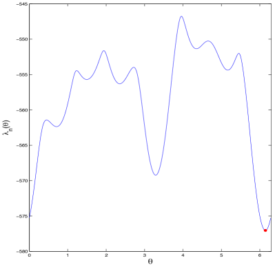
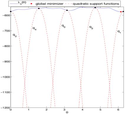
Fig. 2: On the left, the plot of $\lambda_{n}({\mathcal{A}}(\theta))$ for the $400\times 400$ Poisson example (Example 1) with respect to $\theta$; On the right, the plot of $\lambda_{n}({\mathcal{A}}(\theta))$ together with the first five quadratic support functions $q_{j},\;j=0,\dots,4$ formed. In both figures, the asterisk represents the global minimizer, the squares on the right mark the iterates of the algorithm around which the support functions are constructed.

$n$	400	900	1600	2500	3600
eigopt	14	103	328	1079	2788
level-set	17	181	1477	–	–

Table 2: CPU times (in seconds) required by Algorithm 1 (eigopt) and the specialized level-set approach in [32] to compute the numerical radius of Poisson matrices of varying size $n$.

Example 2 (Distance to Uncontrollability): Next, we consider the distance to uncontrollability defined and motivated in Section 2.1. Here, for a given linear system $\;\;x^{\prime}(t)=Ax(t)+Bu(t),\;\;$ where $A\in{\mathbb{C}}^{n\times n},B\in{\mathbb{C}}^{n\times m}$ are such that $n\geq m$, the smallest singular value of ${\mathcal{A}}(z)=\left[\begin{array}[]{cc}A-zI&B\end{array}\right]$ is sought to be minimized over $z\in{\mathbb{C}}$. We again assume generic simplicity, that is the multiplicity of $\sigma_{n}(z):=\sigma_{n}\left({\mathcal{A}}(z)\right)$ is one for all $z$. This property holds on a dense subset of all pairs $(A,B)$. In this case, expressions for the gradient is given by (11). In particular, denoting a consistent pair of unit left and right singular vectors associated with $\sigma_{n}(z)$ by $u_{n}(z)\in{\mathbb{C}}^{n},v_{n}(z)=\left[\begin{array}[]{c}\tilde{v}_{n}(z)\\ \hat{v}_{n}(z)\\ \end{array}\right]\in{\mathbb{C}}^{n+m}$ where $\tilde{v}_{n}(z)\in{\mathbb{C}}^{n},\hat{v}_{n}(z)\in{\mathbb{C}}^{m}$, we have

$$\nabla\sigma_{n}(z)=\left(\frac{\partial\sigma_{n}(z)}{\partial\Re z},\frac{\partial\sigma_{n}(z)}{\partial\Im z}\right)=\left(\;-\Re\left(u_{n}^{\ast}(z)\tilde{v}_{n}(z)\right),\;\Im\left(u_{n}^{\ast}(z)\tilde{v}_{n}(z)\right)\;\right).$$

Furthermore, $\gamma=-4$ appears to be a good lower bound for $\lambda_{\min}\left(\nabla^{2}\sigma_{n}(z)\right)$ numerically. We perform tests on linear systems $(A,B)$ arising from a discretization of the heat equation, taken from the SLICOT library, see [25, Example 3.2]. The matrix $A$ is real, symmetric, tridiagonal, and $n\times n$, whereas $B$ is real and $n\times 1$.

In Table 3, the number of function evaluations required by global optimization algorithms for Lipschitz continuous functions, and Algorithm 1 are presented when the order of the system satisfies $n=30$. The Piyavskii-Shubert algorithm is omitted, because it would be based on locating global minimizers of piecewise cones, and it is not immediate how one would locate these minimizers. Once again, the number of function evaluations for Algorithm 1 seems to suggest linear convergence.

The progress of the algorithm can be traced from the graph associated with it. Recall that the box is split into subregions (indeed polytopes). Inside each subregion, one of the quadratic support functions dominates the others. For the heat equation example of order $n=30$, these graphs are provided after 60, 360, and 580 iterations in Figure 3 in the top three plots. The bottom plot in Figure 3 is an illustration of the level sets of $\sigma_{n}(z)$ in the complex plane along with the computed global minimizer (accurate up to 13 decimal digits after 589 function evaluations) marked with an asterisk. The box is split into subregions more or less uniformly initially, e.g., after 60 iterations. However, later iterations form finer subregions around minimizers of $\sigma_{n}(z)$.

We also compare Algorithm 1 with the level-set approach in [20] on the heat equation examples of varying order. The level set approaches become prohibitively expensive as the number of optimization parameters increases. Here, with the minimization over two parameters, it requires the solutions of eigenvalue problems of size $n^{2}$ for a system of order $n$. For small systems, the level-set approach works very well, however, even for medium-scale systems it becomes computationally infeasible. This is illustrated in Table 4. On the other hand, Algorithm 1 is capable of solving even a problem of order 1000 in a reasonable amount of time.

$\epsilon$	$10^{-2}$	$10^{-4}$	$10^{-6}$	$10^{-8}$	$10^{-10}$	$10^{-12}$
eigopt	520	531	543	556	572	585
brute force	$4.2\times 10^{6}$	$4.2\times 10^{10}$	$4.2\times 10^{14}$	$4.2\times 10^{18}$	$4.2\times 10^{22}$	$4.2\times 10^{26}$
DIRECT	37781	37867	37867	38233	38441	38805

Table 3: Number of function evaluations by various algorithms to compute the distance to uncontrollability for the linear system $(A,B)$ arising from the heat equation [25, Example 3.2], where $A\in{\mathbb{R}}^{30\times 30}$, $B\in{\mathbb{R}}^{30\times 1}$ with respect to absolute accuracy $\epsilon$.

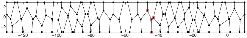
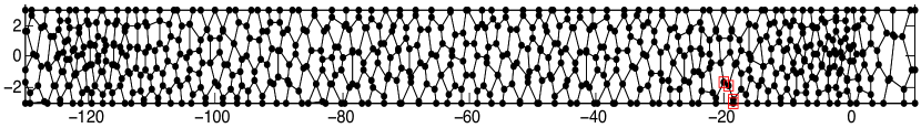
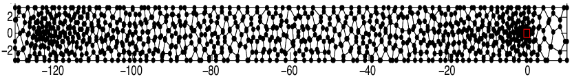
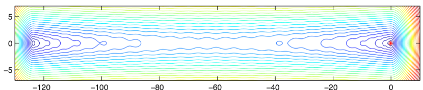
Fig. 3: The top three plots display the graph associated with Algorithm 1 after 60, 360, and 580 iterations to compute the distance to uncontrollability for the heat equation example [25, Example 3.2] of order $n=30$ (see Example 2). The red squares correspond to dead vertices. The bottom plot displays the level sets of $\;\sigma_{n}(z)$ for the same heat equation example together with the computed global minimizer marked with an asterisk.

$n$	30	60	100	200	400	1000
eigopt	45	46	56	85	119	384
level-set	20	393	–	–	–	–

Table 4: CPU times (in seconds) required by Algorithm 1 (eigopt) and the level-set approach in [20] to compute the distance to uncontrollability for the heat equation examples (Example 2) with respect to the order of the system $n$.

Example 3 (Minimizing the Largest Eigenvalue, Convex): This example is taken from [13], and concerns the minimization of the largest eigenvalue of an affine matrix function of the form

$${\mathcal{A}}(\omega)=A_{0}+\sum_{j=1}^{5}\omega_{j}A_{j},$$

depending on five parameters, where $A_{j}\in{\mathbb{R}}^{5\times 5},\;j=0,\dots,5$, are real, symmetric and as in [13], where the minimal value of $\lambda_{1}(\omega):=\lambda_{1}({\mathcal{A}}(\omega))$ is cited as $0.708882597$. Whenever ${\mathcal{A}}(\omega)$ is affine, the largest eigenvalue $\lambda_{1}(\omega)$ is convex by Theorem 6 (see also [14, Theorem A.1]), so we set $\gamma=0$. Thus, this eigenvalue optimization problem can be posed as a semi-definite program (SDP), and solved by means of interior-point methods [34]. The purpose here is to compare the performances of Algorithm 1, and DIRECT method on a multi-dimensional example for which the solution is known (even though our algorithm is really devised for non-convex problems, and in all likelihood an interior-point method would outperform it in the convex case).

This comparison is provided in Table 5, where we again observe linear convergence of Algorithm 1. DIRECT method is not suitable even for a few decimal-digit precision. Indeed, even after 500,000 function evaluations and 3732 seconds of CPU time, it cannot achieve six decimal-digit accuracy. In contrast to the one-dimensional and two-dimensional examples, keeping the graph structure properly, in particular forming the adjacencies between the new vertices, take almost all of the computational time rather than the function evaluations. Even if the matrices $A_{j}$ were much bigger than $5\times 5$, the computation times would not be affected significantly. Therefore, in the table, the CPU times (in seconds) are also provided in parenthesis.

The later iterations are more expensive, since the number of new vertices created increases at the later iterations. Up to four dimensions, the increase in the number of vertices at every iteration seems more or less fixed. In contrast, this does not hold when the dimension is five or more. (These observations are solely based on numerical experiments; we do not have a clear understanding of this phenomenon at the moment.) This is illustrated for the affine example with five parameters in Figure 4. In the figure on the left, the solid and dashed lines represent the number of dead vertices and the number of newly added vertices, respectively, at iterations $1,2,\dots,107$. The graph indicates an increase in both the number of dead vertices and the number of new vertices with respect to the iteration. However, the increase in the number of new vertices is larger. On the right, the total number of vertices is displayed with respect to the iteration number. The graph reveals that the number of vertices seems to increase superlinearly.

$\epsilon$	$10^{-2}$	$10^{-4}$	$10^{-6}$	$10^{-8}$	$10^{-10}$	$10^{-12}$
eigopt	17 (34)	34 (203)	50 (501)	67 (1021)	87 (2040)	108 (3725)
DIRECT	459	45937	–	–	–	–

Table 5: Number of function evaluations by Algorithm 1 (eigopt) and DIRECT method for minimizing the largest eigenvalue of the affine matrix function (Example 3) with respect to absolute accuracy $\epsilon$. The CPU times for eigopt (in seconds) are also provided in parentheses.

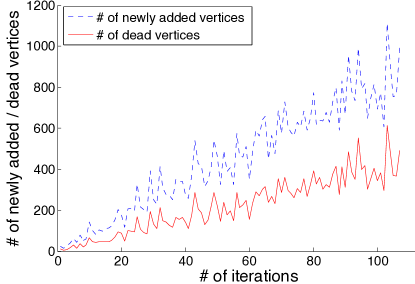
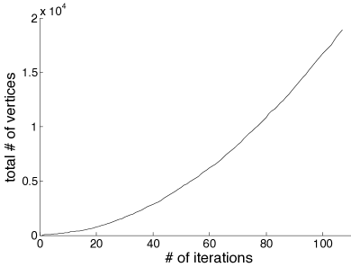
Fig. 4: On the left, the number of dead vertices (solid line) and the number of newly added vertices (dashed line) with respect to the iteration number are displayed, whereas on the right, the total number of vertices with respect to the iteration number is displayed for Example 3.

Example 4 (Minimizing the Largest Eigenvalue, Non-convex): This is a non-convex example depending on four parameters, involving the minimization of the largest eigenvalue of the matrix function

$${\mathcal{A}}(\omega)=A_{0}+\sum_{j=1}^{4}\omega_{j}A_{j}+\frac{1}{2}\sum_{j=1}^{4}\sum_{k=1}^{4}\omega_{j}\omega_{k}A_{jk},$$ (31)

where $A_{0},A_{1},\dots,A_{4}$ are as in the previous affine example taken from [13], while $A_{jk}$ are randomly chosen $5\times 5$ symmetric and real matrices such that $A_{jk}=A_{kj}$. By Corollary 7, a lower bound for $\lambda_{\min}\left(\nabla^{2}\lambda_{1}\left({\mathcal{A}}(\omega)\right)\right)$ is given by $\gamma=\lambda_{\min}\left(\nabla^{2}{\mathcal{A}}\right)$ where $\nabla^{2}{\mathcal{A}}\in{\mathbb{R}}^{20\times 20}$, and $A_{jk}$ constitutes the $5\times 5$ submatrix of $\nabla^{2}{\mathcal{A}}$ at rows $5(j-1)+1:5j$ and columns $5(k-1)+1:5k$. Table 6 displays a comparison of the number of function evaluations for Algorithm 1 and DIRECT method with respect to accuracy. As usual, Algorithm 1 seems to exhibit linear convergence.

$\epsilon$	$10^{-2}$	$10^{-4}$	$10^{-6}$	$10^{-8}$	$10^{-10}$	$10^{-12}$
eigopt	52	141	225	309	391	472
DIRECT	45	161	369	939	1367	2049

Table 6: Number of function evaluations by Algorithm 1 (eigopt) and DIRECT method for minimizing the largest eigenvalue of the matrix function (31) with respect to absolute accuracy $\epsilon$.

10 Software

A MATLAB implementation of Algorithm 1 is available on the web. The implementation makes use of heaps, adjacency lists, stacks, and updates the underlying graph structure efficiently. The user is expected to write down a MATLAB routine that calculates the eigenvalue function and its gradient at a given point. The name of this routine and $\gamma$, a global lower bound on the minimum eigenvalues of the Hessians of the eigenvalue functions must be supplied by the user. We refer to the web page associated with this implementation, where a user guide is also provided.

11 Conclusion

The analytical properties of eigenvalues of matrix-valued functions facilitate the use of so-called quadratic support functions that globally underestimate the eigenvalue curves for their optimization. This observation motivates the idea of adapting support function based global optimization approaches, especially the approach due to Breiman and Cutler [4], for non-convex eigenvalue optimization. In this paper, we illustrated how such global optimization approaches based on the derivative information could be realized in the context of non-convex eigenvalue optimization. We derived the necessary quadratic support functions, elaborated on deducing analytical global lower bounds $\gamma$ for the second derivatives of the extreme eigenvalue functions, which are essential for the algorithm, and provided a global convergence proof. The algorithm is especially applicable for the optimization of extreme eigenvalues, for instance, for the minimization of the largest eigenvalue, and those eigenvalue functions that exhibit generic simplicity.

Acknowledgements We thank two anonymous referees for their invaluable comments, which improved this paper considerably. We are also grateful to Michael Karow and Melina Freitag for helpful discussions and feedback.

References

• [1] O. Axelsson, H. Lu, and B. Polman. On the numerical radius of matrices and its application to iterative solution methods. Linear and Multilinear Algebra, 37:225–238, 1994.
• [2] D. Barnes. The shape of the strongest column is arbitrarily close to the shape of the weakest columns. Quart. Appl. Math., XLIV:605–609, 1986.
• [3] S. Boyd and V. Balakrishnan. A regularity result for the singular values of a transfer matrix and a quadratically convergent algorithm for computing its ${\bf L}_{\infty}$-norm. Systems Control Lett., 15(1):1–7, 1990.
• [4] L. Breiman and A. Cutler. A deterministic algorithm for global optimization. Math. Program., 58(2):179–199, February 1993.
• [5] N.A. Bruinsma and M. Steinbuch. A fast algorithm to compute the ${H}_{\infty}$-norm of a transfer function matrix. Systems Control Lett., 14:287–293, 1990.
• [6] R. Byers. A bisection method for measuring the distance of a stable matrix to the unstable matrices. SIAM J. Sci. Stat. Comp., 9:875–881, 1988.
• [7] R. Byers. The descriptor controllability radius. In Numerical Methods Proceedings of the International Symposium MTNS-93, volume II, pages 85–88. Uwe Helmke, Reinhard Mennicken, and Hosef Saurer, eds., Akademie Verlag, Berlin, 1993.
• [8] S.J. Cox and M.L. Overton. On the optimal design of columns against buckling. SIAM J. Math. Anal., 23:287–325, 1992.
• [9] J. Cullum, W.E. Donath, and P. Wolfe. The minimization of certain nondifferentiable sums of eigenvalues of symmetric matrices. Math. Program Study, 3:35–55, 1975.
• [10] W.E. Donath and A.J. Hoffman. Lower bounds for the partitioning of graphs. IBM J. Res. Dev., 17(5):420–425, September 1973.
• [11] M. Eiermann. Field of values and iterative methods. Linear Algebra Appl., 180:167–197, 1993.
• [12] R. Eising. Between controllable and uncontrollable. Systems Control Lett., 4(5):263–264, 1984.
• [13] M.K.H. Fan and B. Nekooie. On minimizing the largest eigenvalue of a symmetric matrix. Linear Algebra Appl., 214(0):225 – 246, 1995.
• [14] R. Fletcher. Semidefinite matrix constraints in optimization. SIAM J. Control Optim., 23:493–513, 1985.
• [15] M.A. Freitag and A. Spence. A Newton-based method for the calculation of the distance to instability. Linear Algebra Appl., 435(12):3189–3205, 2011.
• [16] S. Friedland, J. Nocedal, and M.L. Overton. The formulation and analysis of numerical methods for inverse eigenvalue problems. SIAM J. Numer. Anal., 24(3):pp. 634–667, 1987.
• [17] M. Gao and M. Neumann. A global minimum search algorithm for estimating the distance to uncontrollability. Linear Algebra Appl., 188-189:305–350, 1993.
• [18] V.P. Gergel. A global optimization algorithm for multivariate functions with Lipschitzian first derivatives. J. Global Optim., 10(3):257–281, 1997.
• [19] M. Gu. New methods for estimating the distance to uncontrollability. SIAM J. Matrix Anal. Appl., 21(3):989–1003, 2000.
• [20] M. Gu, E. Mengi, M.L. Overton, J. Xia, and J. Zhu. Fast methods for estimating the distance to uncontrollability. SIAM J. Matrix Anal. Appl., 28(2):477–502, 2006.
• [21] C. He and G.A. Watson. An algorithm for computing the distance to instability. SIAM J. Matrix Anal. Appl., 20:101–116, 1999.
• [22] D. Hinrichsen and M. Motscha. Optimization problems in the robustness analysis of linear state space systems. In Proceedings of the International Seminar on Approximation and Optimization, pages 54–78, New York, NY, USA, 1988. Springer-Verlag New York, Inc.
• [23] R.A. Horn and C.R. Johnson. Topics in Matrix Analysis. Cambridge University Press, 1991.
• [24] D. R. Jones, C. D. Perttunen, and B. E. Stuckman. Lipschitzian optimization without the Lipschitz constant. J. Optim. Theory Appl., 79(1):157–181, 1993.
• [25] D. Kressner, V. Mehrmann, and T.Penzl. Ctdsx - a collection of benchmarks for state-space realizations of continuous-time dynamical systems. SLICOT Working Note, 1998.
• [26] D.E. Kvasov and Ya.D. Sergeyev. A univariate global search working with a set of Lipschitz constants for the first derivative. Optimization Lett., 3(2):303–318, 2009.
• [27] D.E. Kvasov and Ya.D. Sergeyev. Lipschitz gradients for global optimization in a one-point-based partitioning scheme. J. Comput. Appl. Math., 236(16):4042 – 4054, 2012.
• [28] P. Lancaster. On eigenvalues of matrices dependent on a parameter. Numer. Math., 6:377–387, 1964.
• [29] D. Lera and Ya.D. Sergeyev. Acceleration of univariate global optimization algorithms working with Lipschitz functions and Lipschitz first derivatives. SIAM J. Optimization, 23(1):508 – 529, 2013.
• [30] A.S. Lewis and M.L. Overton. Eigenvalue optimization. Acta Numer., 5:149–190, 0 1996.
• [31] M. Mäkelä. Survey of bundle methods for nonsmooth optimization. Optim. Method. Softw., 17(1):1–29, 2002.
• [32] E. Mengi and M.L. Overton. Algorithms for the computation of the pseudospectral radius and the numerical radius of a matrix. IMA J. Numer. Anal., 25:648–669, 2005.
• [33] M. Myers and W. Spillers. A note on the strongest fixed-fixed column. Quart. Appl. Math., XLIV:583–588, 1986.
• [34] Y. Nesterov and A. Nemirovski. Interior point polynomial methods in convex programming. SIAM, Philadelphia, 1994.
• [35] N. Olhoff and S. Rasmussen. On single and bimodal optimum buckling loads of clamped columns. Int. J. Solids Struct., 13(7):605 – 614, 1977.
• [36] M.L. Overton. On minimizing the maximum eigenvalue of a symmetric matrix. SIAM J. Matrix Anal. Appl., 9(2):256–268, April 1988.
• [37] M.L. Overton. Large-scale optimization of eigenvalues. SIAM J. Optimization, 2:88–120, 1991.
• [38] M.L. Overton and R.S. Womersley. Second derivatives for optimizing eigenvalues of symmetric matrices. SIAM J. Matrix Anal. Appl., 16(3):697–718, July 1995.
• [39] C.C. Paige. Properties of numerical algorithms relating to computing controllability. IEEE Trans. Automat. Control, 26:130–138, 1981.
• [40] S. A. Piyavskii. An algorithm for finding the absolute extremum of a function. USSR Comput. Math. and Math. Phys., 12:57–67, 1972.
• [41] F. Rellich. Perturbation Theory of Eigenvalue Problems. Gordon and Breach, 1969.
• [42] Ya.D. Sergeyev. Multidimensional global optimization using the first derivatives. Comp. Math. Math. Phys+., 39(5):743 – 752, 1999.
• [43] Y.D. Sergeyev and D.E. Kvasov. Global search based on efficient diagonal partitions and a set of Lipschitz constants. SIAM J. Optimization, 16(3):910–937, 2006.
• [44] A. Shapiro and M.K.H. Fan. On eigenvalue optimization. SIAM J. Optimization, 5:552–569, 1995.
• [45] B. Shubert. A sequential method seeking the global maximum of a function. SIAM J. Numer. Anal., 9:379–388, 1972.
• [46] I. Tadjbakhsh and J.B. Keller. Stringest columns and isoperimetric inequalities for eigenvalues. J. Appl. Mech., 29(1):159–164, 1962.
• [47] C. F. Van Loan. How near is a matrix to an unstable matrix? Lin. Alg. and its Role in Systems Theory, 47:465–479, 1984.
• [48] C.T.C. Wall. Singular Points of Plane Curves. Cambridge University Press, Cambridge, 2004.