Functional-integral approach to the investigation of the spin-spiral magnetic order and phase separation

Keywords: Hubbard model, spiral magnetic phases, phase separation, superconducting.

Abstract. We investigate a two–dimensional single-band Hubbard model with a nearest–neighbor hopping. We treat a commensurate collinear order as well as incommensurate spiral magnetic phases at a finite temperature using a Hubbard–Stratonovich transformation with a two–field representation and solve this problem in a static approximation. We argue that temperature dramatically influence the collinear and spiral magnetic phases, phase separation in the vicinity of half–filling. The results imply a possible interpretation of unusual behavior of magnetic properties of single–layer cuprates.

1 Introduction

Investigation of two–dimensional (2D) electronic systems attracts substantial interest, which has been stimulated by the discovery of high-temperature superconducting cuprates. It is generally accepted that superconducting and magnetic propeties of cuprates are closely related, but magnetic properties are formed by $Cu$–layers and interlayer coupling is weak. At half–filling, the cuprates are antiferromagnetically ordered, evolution of their magnetic properties with doping and temperature is an interesting challenge. For example, neutron scattering in $La_{2-x}Sr_{x}CuO_{4}$ reveals coexistence of both commensurate and incommensurate magnetic structures in the vicinity of half–filling at low temperature, that pass to antiferromagnetic with rise of temperature [1, 2, 3, 4]. Recently the authors [5] considered the ground–state magnetic phase diagram of the two–dimensional single-band Hubbard model with nearest and next–nearest–neighbor hopping in terms of electronic density and interaction. They treated commensurate ferromagnetic and antiferromagnetic as well as incommensurate spiral magnetic phases using the mean field (MF) approximation. First–order magnetic transitions with changing chemical potential, resulting in a phase separation (PS) in terms of density, was found between ferromagnetic, antiferromagnetic, and spiral magnetic phases.

Here phase diagram is investigated depending on temperature. Our calculations are based on a two–dimensional single–band Hubbard model. We use a Hubbard–Stratonovich transformation with a two–field representation and solve this problem in a static approximation. It allows us, on the one hand, to obtain a solution that coincides with the MF approximation at zero temperature and, on the other hand, to investigate the temperature behavior of PS and phase transformation taking into account thermodynamic transverse spin fluctuations.

First of all, we want to emphasize the peculiarity of the 2D magnetic systems. The series of works proved rather directly impossibility of existence of a spontaneous magnetic order and phase separation in a two-dimensional Hubbard model [6, 7, 8] (at finite temperature the results [6, 7] coincide with Mermin’s theorem). At the same time, there are a lot of papers using the 2D Hubbard model for describing cuprates (see, for example, [9, 10, 11, 12] and references in them). Usually, it is believed that weak interlayer coupling stabilizes a magnetic order, which allows us to consider fluctuations around this broken-symmetry state even at finite temperature. Therefore, one can choose approximations which depress the 2D divergence of magnetic fluctuations (for example, a mean field approximation, a dynamic mean field approximation and so on). In addition, phase separation and inhomogeneous magnetic state in the 2D Hubbard model have been obtained recently by calculation methods using an extension of the dynamic mean-field theory and advances in a quantum Monte Carlo techniques [9, 10, 11]. We want to emphasize that exact results of [6, 7, 8] were received for homogeneous states; therefore, for inhomogeneous case the long wave fluctuations are cut off for the mean length of homogeneity. It reminds the stability of a 2D graphene layer where «ripples» appear due to thermal and quantum fluctuations and this stabilizes the crystal [13]. Though the problems of a 2D-crystal stability and of an inhomogeneous magnetic order in the 2D Hubbard model have not been solved yet, the results of the calculation methods give us an additional basis for using approximations which stabilize states with a broken symmetry. In this paper we neglect magnetic longitudinal fluctuations and thereby depress the 2D divergence.

2 Method

We consider the Hamiltonian of the Hubbard model on the square lattice ${\hat{H}}={\hat{H}}_{0}+{\hat{H}}_{int},\,$

$${\hat{H}}_{0}=\sum_{i,j,s}t_{ij}\hat{c}_{i,s}^{+}\hat{c}_{j,s},\,\quad{\hat{H}}_{int}=U\sum_{j}\hat{c}_{j,\uparrow}^{+}\hat{c}_{j,\uparrow}\hat{c}_{j,\downarrow}^{+}\hat{c}_{j,\downarrow},\,$$ (1)

where $j$ is a number of site, $s$ is a spin projection, $t_{ij}=-t$ for the nearest–neighbor site and $0$ if not, $\hat{c}_{j,s}(\hat{c}_{j,s}^{+})$ is a creation (annihilation) electronic operator on the site $j$ and $U$ is the electronic (Hubbard) on–site interaction. We use a two-field formalism in the Hubbard-Stratonovich transformation, therefore more convenient representation of the on-site interaction in form

$${\hat{H}}_{int}=U\sum_{j}\hat{n}_{j,\uparrow}\hat{n}_{j,\downarrow}=U\sum_{j}\left[\hat{n}_{j}^{2}/4-(\vec{\hat{S}}_{j}\cdot\vec{e}_{j})^{2}\right],\,$$ (2)

where $\vec{e}_{j}$ is the (arbitrarily chosen) $j$–dependent unit vector and we introduce the site density $\hat{n}_{j,s}=\hat{c}_{j,s}^{+}\hat{c}_{j,s}$, $\hat{n}_{j}=\hat{n}_{j,\uparrow}+\hat{n}_{j,\downarrow}$ and the site magnetization operator $\vec{{\hat{S}}}_{j}=1/2\sum_{s,s^{\prime}}\hat{c}_{j,s}^{+}\vec{\sigma}_{s,s^{\prime}}\hat{c}_{j,s}$, ($\vec{\sigma}_{s,s^{\prime}}$ are the elements of vector $\vec{\sigma}=(\sigma_{x},\,\sigma_{y},\,\sigma_{z})$ formed by the Pauli spin matrices).

Thermodynamical properties are defined by partition function of the grand canonical ensemble:

$$Z=Tr\left[\exp\left\{-\beta({\hat{H}}-\mu{\hat{n}}\right\}\right]=Tr\left[\exp\left\{-\beta({\hat{H}}_{0}-\mu{\hat{n}})\right\}T_{\tau}\exp\left\{-\int_{0}^{\beta}{\hat{H}}_{int}(\tau)d\tau\right\}\right].\,$$ (3)

Here $\mu$ is a chemical potential, $T_{\tau}$ is a time ordering operator, $Tr$ is summation over a complete set of states, ${\hat{H}}_{int}(\tau)=\exp{(-\tau{\hat{H}}_{0})}{\hat{H}}_{int}\exp{(\tau{\hat{H}}_{0})}$ is an operator in the interaction representation, $\beta=1/k_{B}T$, $T$ is temperature. Partition function can be rewrite with the help of a Hubbard–Stratonovich transformation

$$Z=\int\prod_{i}D{\vec{v}}_{j}(\tau)D\zeta_{j}(\tau)Z[{\vec{v}},\zeta],$$ (4)

$$Z[{\vec{v}},\zeta]=\exp{\left\{-\beta F({\vec{v}},\zeta)\right\}}=\exp{\left\{-U\sum_{j}\int_{0}^{\beta}d\tau[{\vec{v}}_{j}^{2}(\tau)+\zeta_{j}^{2}(\tau)]\right\}}Z^{*}[{\vec{v}},\zeta],\,$$

$$Z^{*}[{\vec{v}},\zeta]=Tr\left[\exp{\left\{-\beta({\hat{H}}_{0}-\mu{\hat{n}})\right\}}T_{\tau}\exp{\left\{-\sum_{j}\int_{0}^{\beta}d\tau{\hat{V}}_{jj}({\vec{v}},\zeta,\tau)\right\}}\right],\,$$

$${\hat{V}}_{jj}({\vec{v}},\zeta,\tau)=U\left[i\zeta_{j}(\tau)\hat{n}_{j}(\tau)-2\vec{v}_{j}(\tau)\cdot\vec{{\hat{S}}}_{j}(\tau)\right],\,\qquad\qquad$$

here ${\vec{v}}_{j}$ and $\zeta_{j}$ are auxiliary fields connected with spin and charge on the site $j$.

We consider the spiral type of incommensurate magnetic order, which is the rotation of order parameter in the plane, modulated with some wave vector ${\vec{Q}}=(Q_{x},Q_{y})$ (the superposition states of the rotation and the ferromagnetic component perpendicular to the plane have high energy [14]). These states coincide with MF approximation states at zero temperature [5]

$${\vec{e}}_{j}={\vec{e}}_{x}\cos{({\vec{Q}}{\vec{R}}_{j})}+{\vec{e}}_{y}\sin{({\vec{Q}}{\vec{R}}_{j})}.\,$$ (5)

The two-field formalism allows us to obtain a Hartree-Fock approximation in the limit of vanishing temperature [15] and phase separation [5]. From here it is more convenient for us to make an identical transformation and to denote

$${\hat{\cal H}}_{0}=\sum_{{\vec{k}}}{\cal E}_{{\vec{k}},\uparrow}\hat{c}_{{\vec{k}},\uparrow}^{+}\hat{c}_{{\vec{k}},\uparrow}+{\cal E}_{{\vec{k}},\downarrow}\hat{c}_{{\vec{k}},\downarrow}^{+}\hat{c}_{{\vec{k}},\downarrow}-UM\sum_{{\vec{k}}}\left(\hat{c}_{{\vec{k}},\uparrow}^{+}\hat{c}_{{\vec{k}}+{\vec{Q}},\downarrow}+\hat{c}_{{\vec{k}}+{\vec{Q}},\downarrow}^{+}\hat{c}_{{\vec{k}},\uparrow}\right),$$ (6)

$${\hat{\cal H}}_{int}=U\sum_{j}\left[\left(\hat{n}_{j}-n_{e}\right)^{2}/4-\left({\vec{\hat{S}}}_{j}\cdot\vec{e}_{j}-M\right)^{2}\right],\,$$

with ${\cal E}_{{\vec{k}},\uparrow(\downarrow)}={\cal E}_{{\vec{k}}}+Un_{e}/2$, ${\cal E}_{{\vec{k}}}=-2t(\cos{k_{x}}+\cos{k_{y}})$, where $n_{e}$ is a density and $M$ is a magnetization. Introducing Green function for ${\hat{G}}_{0}(z)=(z-{\hat{\cal H}}_{0})^{-1}$ and making a standard calculation [16] we obtain

$$Z^{*}[{\vec{v}},\zeta]=\exp{\left\{-\beta\Omega({\vec{v}},\zeta)\right\}},\qquad\Omega({\vec{v}},\zeta)=\Omega_{0}-\frac{1}{\beta}\sum_{n,j}Tr\ln{[1-G_{jj}^{0}(i\omega_{n})V_{jj}({\vec{v}},\zeta)]}.$$ (7)

Here $\Omega_{0}=-1/\beta\ln{Tr\exp{[-\beta({\hat{H}}_{0}-\mu{\hat{n}})]}}$ is a thermodynamical potential of noninteracting electrons, $\omega_{n}=\pi(2n+1)/\beta$ are fermion Matsubara frequencies, $n=0,\pm 1,...$, $V_{jj}$ and ${G}_{jj}^{0}$ are matrices of spin variables. For simplification of the expression (4) we use the static approximation assuming that ${\vec{v}}_{i}(\tau)$ and $\zeta(\tau)$ are independent on $\tau$. We neglect the thermal fluctuation of the charge field $\zeta_{j}$. Thus, for each configuration of the spin field ${\vec{v}}_{j}$ we set $\zeta_{j}^{0}({\vec{v}}_{j})$ equal to the saddle point that is given by equation

$$\qquad\qquad\frac{\partial F({\vec{v}},\zeta)}{\partial\zeta_{j}}=U\left[-2\zeta_{j}+in_{j}({\vec{v}_{j},\zeta_{j}})\right]=0,\qquad\zeta_{j}^{0}({\vec{v}}_{j})=in_{j}({\vec{v}}_{j},\zeta_{j}^{0})/2,$$

$$n_{j}({\vec{v}}_{j},\zeta_{j})=\frac{1}{\beta}\sum_{n}Tr\left\{\left[1-G_{jj}^{0}(i\omega_{n})V_{jj}({\vec{v}},\zeta)\right]^{-1}G_{jj}^{0}(i\omega_{n})\right\}.\qquad$$ (8)

We neglect longitudinal and leave only transverse fluctuations implying ${\vec{v}}_{j}=v\cdot{\vec{e}}_{j}$. We want to emphasize that ${\vec{e}}_{j}$ is the (arbitrarily chose) $j$-dependent unit vector. At last, we change the matrix expression $(1-G_{jj}^{0}V_{jj})^{-1}G_{jj}^{0}$ for the average Green function ${\tilde{G}}(z)$ (averaging is conducted over transverse fluctuations of auxiliary field $v$ $<...>_{v}$ ). The self-energy $\Sigma(z)$ and ${\tilde{G}}(z)$ is found from the self-consistency equation treatment by a coherent-potential approximation (CPA)

$${\tilde{G}}_{jj}(z)=<\left[1-G_{jj}^{0}(z)V_{jj}(v)\right]^{-1}G_{jj}^{0}(z)>_{v}=G_{jj}^{0}(z-\Sigma(z)).$$ (9)

At last we can write partition function in terms integration over $v$

$$Z=\int dv\exp{\left\{-\beta U\left[v^{2}+\zeta^{2}(v)\right]\right\}}\exp{\left\{-\beta\Omega(v)\right\}},$$ (10)

$$\Omega(v)=\Omega_{0}+\frac{1}{\beta}\sum_{n}\left\{ln{\,det[1-{\tilde{G}}(i\omega_{n})(V(v)-\Sigma(i\omega_{n}))]}-ln{\,det[1+\Sigma(i\omega_{n}){\tilde{G}}(i\omega_{n})]}\right\}.$$

For short of the expression (10) we miss out site index $j$.

Self-consistence solution of the Eqs.(2),(9),(10) allows us to calculate all magnetic properties of our system.

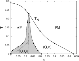
Figure 1: Magnetic phase diagram for $U/t=4$. Bold lines denote the temperature Neel (second-order phase transitions), solid lines denote boundaries of phase-separated region AF+ $(Q,\pi)$ (shaded area), dashed lines denote first-order phase transitions calculated without regard for PS.

Figure 2:

Figure 3:

3 Results

We have performed numerical calculations comparing thermodynamical potential of different magnetic phases at different $n$ and $T$, solving the Eqs. (2),(9),(10) for $U/t=4$. Hamiltonian (1) have the particle-hole symmetry $(n\leftrightarrow 2-n)$ and we can restrict ourselves to the region $0\leq n\leq 1$. The magnetic phase diagram is presented in Fig. 1. At zero temperature the antiferromagnetic (AF) phase exist only at half-filling $(n=1)$ [5, 14]. The region of AF states is intensively grown with temperature. The dependences of $Q_{x}$ on $T$ and n are shown in the Fig. 2. We can see that AF $\to(Q,Q)$ phase transition is a first-order transition. From our calculation it is clearly that $(Q,Q)\to(Q,\pi)$ and AF $\to(Q,\pi)$ transitions are also first-order transitions. This is confirmed by the dependence of chemical potential $\mu$ on number of electrons $n$ Fig. 3. We can see two regions of $\mu$ instability AF $\to(Q,Q)$ and $(Q,Q)\to(Q,\pi)$ phases, which are characterized by negative derivative of $\mu$ $(n=(0.92-0.9,0.87-0.86))$. Therefore these regions must consist of two spatially separated phases. Boundaries of PS and proportion of phases can be obtained through the Maxwell construction.

$$\int_{n1}^{n2}\left[\mu(n_{1})-\mu(n)\right]dn=0.\,$$ (11)

The Fig. 3 shows dependence of the chemical potential with account to phase separation.

4 Summary

In summary, our investigations demonstrate that the magnetic phase transition qualitative coincides with experiments, notably the transitions from paramagnetic state to AF one and then to PS at low temperature [1, 2, 3, 4], see Fig. 1. However the phase separates to AF and $(Q,\pi)$ phases, whereas experiment shows separation to AF and $(Q,Q)$ phases and a region of separation to $(Q,Q)$ and $(Q,\pi)$ phases [4]. Behavior of the chemical potential (two regions of instability in Fig. 3) indicates a high possibility of the existence of PS AF $+(Q,Q)$ and $(Q,Q)+(Q,\pi)$ phases at some choice of Hamiltonian parameters (1), in particular with account of a next-nearest-neighbor hopping [5].

5 Acknowledgments

The work is supported No. 09-02-00461 from Russian Basic Research Foundation, and by Program of RAS No. 09–2-2001

References

- [1] C.H. Lee, K. Kurahashi, J. Wada, S. Wakimoto, S. Ueki, H. Kimura, and Y. Endoh: Phys. Rev. Vol. 57 (1998), p. 6165
- [2] M. Matsuda, M. Fujita, K. Yamada, R.J. Birgeneau, M.A. Kastner, H. Hiraka, Y. Endoh, S. Wakimoto, G. Shirane: Phys. Rev. Vol. 62 (2000), p. 9148
- [3] M. Fujita and K. Yamada, H. Hiraka, P.M. Gehring, S.H. Lee, S. Wakimoto, G. Shirane: Phys. Rev. Vol. 65 (2002), p. 064505
- [4] M. Matsuda, M. Fujita, K. Yamada, R.J. Birgeneau, Y. Endoh, G. Shirane: Phys. Rev. B Vol. 65 (2002), p. 134515
- [5] P.A. Igoshev, M.A. Timirgazin, A.A. Katanin, A.K. Arzhnikov, and V.Yu. Irkhin: Phys. Rev. B Vol. 81 (2010), p. 094407
- [6] D.K. Ghosh: Phys. Rev. Lett. Vol. 27 (1971), p. 1584
- [7] G. Su: Phys. Rev. B Vol. 54 (1996), p. R8281
- [8] M.S. Laad: arXiv0810.4416v1 (2008).
- [9] E. Langmann and M. Wallin: Phys. Rev. Lett. Vol. 127 (2007), p. 825
- [10] A. Macridin, M. Jarrell, and Th. Maier: Phys. Rev. B Vol. 74 (2006), p. 085104
- [11] C. Chang and S. Zhang: Phys. Rev. B Vol. 78 (2008), p. 165101
- [12] T. Maier, M. Jarrell, T. Pruschke, M.H. Hettler, Rev. Mod. Phys, Vol. 77 (2005), p. 1027
- [13] A. Fasolino, J.H. Los and M.I. Katsnelson: Nature mat Vol. 78 (2007), p. 2011
- [14] M.A. Timirgazin and A.K. Arzhnikov: Solid State Phenom. Vol. 559 (2009), p. 152-153
- [15] R.F. Hassing, D.M. Esterling: Phys. Rev. B Vol. 7 (1973), p. 432
- [16] S.Q. Wang, W.E. Evenson, and J.R. Schrieffer, Phys. Rev. Lett. Vol. 23 (1969), p. 92