Statistical Physics approach to dendritic computation: the excitable-wave mean-field approximation

Abstract

We analytically study the input-output properties of a neuron whose active dendritic tree, modeled as a Cayley tree of excitable elements, is subjected to Poisson stimulus. Both single-site and two-site mean-field approximations incorrectly predict a non-equilibrium phase transition which is not allowed in the model. We propose an excitable-wave mean-field approximation which shows good agreement with previously published simulation results [Gollo et al., PLoS Comput. Biol. 5(6) e1000402 (2009)] and accounts for finite-size effects. We also discuss the relevance of our results to experiments in neuroscience, emphasizing the role of active dendrites in the enhancement of dynamic range and in gain control modulation.

I Introduction

Computational neuroscience is a growing field of research which attempts to incorporate increasingly detailed aspects of neuronal dynamics in computational models (Bower and Beeman, 1995; Carnevale and Hines, 2009). Since the pioneering work of Hodgkin and Huxley (HH) (Hodgkin and Huxley, 1952), which unveiled how the action potential in the giant squid axon could be described by ordinary differential equations governing the gating of ionic conductances across a membrane patch, the computational modeling of neuronal biophysical processes has been done at several levels, from whole neural networks to dendritic spines and even single ionic channel dynamics (Dayan and Abbott, 2001).

Rall was probably the first to extend conductance-based modeling to dendrites (Rall, 1964), starting what is nowadays a field of its own: the investigation of so-called dendritic computation (Stuart et al., 2008). The main theoretical tool in this enterprise has been cable theory, the extension [via partial differential equations (PDEs)] of the HH formalism to extended systems, which allows one to include spatial information about dendrites such as the variation of channel densities along the trees, different branching patterns etc. (Koch, 1999). The assumption that dendrites are passive elements renders cable theory linear, allowing the application of standard techniques from linear PDEs and yielding insightful analytical results (Koch, 1999). This assumption, however, has been gradually revised since the first experimental evidences that dendrites have nonlinear properties (Eccles et al., 1958). A variety of channels with regenerative properties are now identified which can sustain the propagation of nonlinear pulses along the trees (called dendritic spikes), whose functional role has nonetheless remained elusive (Stuart et al., 2008).

The conditions for the generation and propagation of dendritic nonlinear excitations have been investigated via cable theory (Mel, 1993; Stuart et al., 2008) at the level of a dendritic branchlet. This has proven useful for understanding the specific role of each ionic channel in the dynamical properties of the nonlinear propagation, specially in comparison with experiments, which have mostly been restricted to the injection of current at some point in the neuron (say, a distal dendrite) and the measurement of the membrane potential at another point (say, the soma) (Johnston and Narayanan, 2008; Sjöström et al., 2008). While this limitation is justified by the difficulties of injecting currents and measuring membrane potentials in more than a couple of points in the same neuron, we must remember that neurons in vivo are subjected to a different stimulus regime, with many synaptic inputs arriving with a high degree of stochasticity and generating several dendritic spikes which may propagate and interact.

In this more realistic and highly nonlinear scenario, cable theory, though still having the merit of being able to incorporate as many ionic channels as experiments reveal, becomes analytically untreatable. Being able to reproduce the fine-grained experimental results of a complex system such as a neuron does not imply that the essential aspects of its dynamics will be identified. Or, to put it in a renormalization group parlance, “realistic biophysical modeling” does not allow us to separate the relevant observables from the irrelevant ones that can be eliminated without significantly changing some robust property of the system. In fact, this has been recognized in the neuroscience literature, which has emphasized the need for theoretical support (Reyes, 2001; Herz et al., 2006; London and Häusser, 2005) and witnessed the increase of theoretical papers in the field of dendritic computation (Poirazi and Mel, 2001; Poirazi et al., 2003a, b; Morita, 2009; Coop et al., 2010).

In this context, we have recently attempted to understand the behavior of an active dendritic tree by modeling it as a large network of interacting nonlinear branchlets under spatio-temporal stochastic synaptic input and allowing for the interaction of dendritic spikes (Gollo et al., 2009). With a statistical physics perspective in mind, we have tried to incorporate in the model of each branchlet only those features that seemed most relevant, and have investigated the resulting collective behavior. Thus each excitable branchlet was modeled as a simple 3-state cellular automaton, with the propagation of dendritic spikes occurring with probabilities which depend on direction (to account for the differences between forward- and backward-propagating spikes).

This model has revealed that such a tree performs a highly nonlinear “computation”, being able to compress several decades of input rate intensity into a single decade of output rate intensity. This signal compression property, or enhancement of dynamic range, is a general property of excitable media and has proven very robust against variations in the topology of the medium and the level of modeling, from cellular automata to compartmental conductance-based models (Copelli et al., 2002, 2005; Copelli and Kinouchi, 2005; Furtado and Copelli, 2006; Kinouchi and Copelli, 2006; Copelli and Campos, 2007; Wu et al., 2007; Assis and Copelli, 2008; Ribeiro and Copelli, 2008; Publio et al., 2009; Larremore et al., 2011a, b; Buckley and Nowotny, 2011). Furthermore, the idea that dynamic range can be enhanced in neuronal excitable media has received support from experiments in very different setups (Kihara et al., 2009; Shew et al., 2009), which again suggests that the phenomenon is robust.

Our aim here is to analytically explore the model introduced in Ref. (Gollo et al., 2009) and described in section II. In section III we show that the traditional cluster approximations applied to the system master equations fail to qualitatively reproduce the essential features observed in the simulations and experimental data. We propose a mean-field approximation which circumvents the problems faced by the traditional approach, yielding good agreement with simulations. We conclude in section IV with a discussion of the consequences of our results for neuroscience and the perspectives for future work.

II Modeling an active dendritic tree

The dendritic tree of an isolated neuron contains no loops and divides in two daughter branches at branching points. For instance, Fig. 1 (a) depicts one of Ramon y Cajal’s drawings of a human Purkinje cell, which shows a huge ramification. Measured by the average number $G$ of generations (i.e., the number of branch-doubling iterations the primary dendrite undergoes), the size of the dendritic trees can vary widely. One can think of an active dendritic tree as an excitable medium (Lindner et al., 2004), in which each site represents, for instance, a branching point or a dendritic branchlet connected with two similar sites from a higher generation and one site from a lower generation. Correspondingly, the standard model in this paper is a Cayley tree with coordination number $z=3$ (Gollo et al., 2009). Each site at generation $g$ has a mother branch from generation $g-1$ and generates two daughter branches ($k\equiv z-1=2$) at generation $g+1$. The single site at $g=0$ would correspond to the primary (apical) dendrite which connects with the neuron soma [see Fig. 1(b)]. Naturally, the Cayley tree topology of our model is a crude simplification of a real tree, as attested by the differences between Figs. 1 (a) and 1(b).

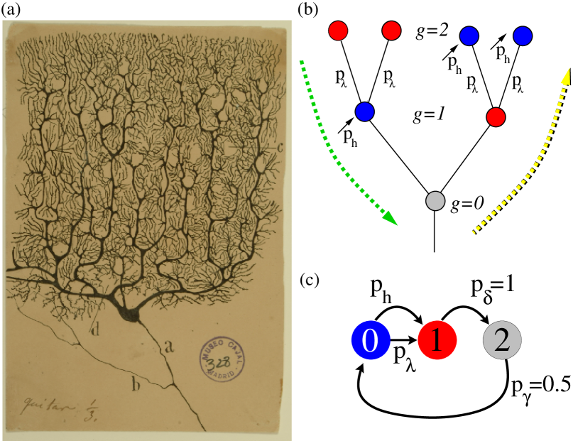
Figure 1: (Color online) Model of an active dendritic tree. (a) A famous drawing by Ramon y Cajal of a human Purkinje cell. (b) Excitable elements (circles) connected (bars) in a Cayley tree topology with $G=2$ layers and coordination number $z=3$ (one mother and $k=2$ daughter branches). Dendritic branchlets are driven by independent Poisson stimuli (small arrows). (c) Each dendritic branchlet can be in one of three states: quiescent (0), active (1) or refractory (2).

Each site represents a dendritic branchlet, which we model with a three-state excitable element (Lindner et al., 2004): $x_{i}(t)\in\{0,1,2\}$ denotes the state of site $i$ at time $t$. If the branchlet is active ($x_{i}=1$), in the next time step it becomes refractory ($x_{i}=2$) with probability $p_{\delta}$. Refractoriness is governed by $p_{\gamma}$, which is the probability with which sites become quiescent ($x_{i}=0$) again [see Fig. 1(c)]. Here we have used $p_{\delta}=1$ and $p_{\gamma}=0.5$. The propagation of dendritic spikes along the tree is assumed to be stochastic as well: each active daughter branch can independently excite its mother branch with probability $p_{\lambda}$, contributing to what is referred to as forward propagation [i.e., from distal dendrites to the soma, see large descending arrow in Fig. 1(b)]. Backpropagating activity is also allowed in the model, with a mother branch independently exciting each of its quiescent daughter branches with probability $\beta p_{\lambda}$ [large ascending arrow in Fig. 1(b)], where $0\leq\beta\leq 1$.

Dendrites are usually regarded as the “entry door” of information for the neuron, i.e., the dominant location where (incoming) synaptic contacts occur. Our aim then is to understand the response properties of this tree-like excitable medium. Incoming stimulus is modeled as a Poisson process: besides transmission from active neighbors (governed by $p_{\lambda}$ and $\beta$), each quiescent site can independently become active with probability $p_{h}\equiv 1-\exp(-h\Delta t)$ per time step [see Fig. 1(c)], where $\Delta t=1$ ms is an arbitrary time step and $h$ is referred to as the stimulus intensity. It reflects the average rate at which branchlets get excited, after the integration of postsynaptic potentials, both excitatory and inhibitory (Gollo et al., 2009). With synchronous update, the model is therefore a cyclic probabilistic cellular automaton.

A variant of the model accounts for the heterogeneous distribution of synaptic buttons along the proximal-distal axis in the dendritic tree. It consists of a layer-dependent rate $h(g)=h_{0}e^{ag}$, with $a$ controlling the nonlinearity of the dependence (Gollo et al., 2009). We will mostly restrict ourselves to the simpler cases $\beta=1$ and $a=0$.

II.1 Simulations

In the simulations, the activity $F$ of the apical ($g=0$) dendritic branchlet is determined by the average of its active state over a large time window ($T=10^{4}$ time steps and 5 realizations). The response function $F(h)$ is the fundamental input-output neuronal transformation in a rate-code scenario (i.e., assuming that the mean incoming stimulus rate and mean output rate carry most of the information the neuron has to transmit).

In a never ending matter of investigation, rate code has historically competed with temporal code, which is also supported by plenty of evidence (Rieke et al., 1997). Auditory coincidence detection (Agmon-Snir et al., 1998), as well as spatial localization properties of place and grid cells fundamentally depend on the precise spike time (Moser et al., 2008). Spike-timing-dependent plasticity, responsible for memory formation and learning, critically relies on small time differences (of order of tens of milliseconds) between presynaptic and postsynaptic neuronal spikes (Bi and Poo, 1998). Moreover, zero-lag or near zero-lag synchronization, which are thought to play an active role in cognitive tasks (Uhlhaas et al., 2009), has been recently shown to be supported and controlled by neuronal circuits despite long connection delays (Fischer et al., 2006; Vicente et al., 2008; Gollo et al., 2010, 2011). Nevertheless, because of its robustness to the high level of stochasticity and trial-to-trial variability present in the brain (Rolls and Deco, 2010), rate code is probably more globally found (Buesing et al., 2011; Rolls and Treves, 2011). In this paper we implicitly assume that rate code holds.

A typical response curve obtained from simulations with $p_{\lambda}=0.7$ and $G=10$ is shown in Fig. 2 (symbols). It is a highly nonlinear saturating curve, with the remarkable property of compressing decades of stimulus intensity $h$ into a single decade of apical response $F$. A simple measure of this signal compression property is the dynamic range $\Delta$, defined as

$$\Delta=10\log\left(\frac{h_{90}}{h_{10}}\right)\;,$$ (1)

where $h_{x}\equiv F^{-1}(F_{x})$ is the stimulus value for which the response reaches $x\%$ of its maximum range: $F_{x}\equiv F_{min}+\frac{x}{100}(F_{max}-F_{min})$, where $F_{min}=\lim_{h\to 0}F(h)$ and $F_{max}=\lim_{h\to\infty}F(h)$. As exemplified in Fig. 2, $\Delta$ amounts to the range of stimulus intensities (measured in dB) which can be appropriately coded by $F$, discarding stimuli which are either so weak as to be hidden by the self-sustained activity of the system ($F<F_{10}$) or so strong that the response is, in practice, non-invertible owing to saturation ($F>F_{90}$).

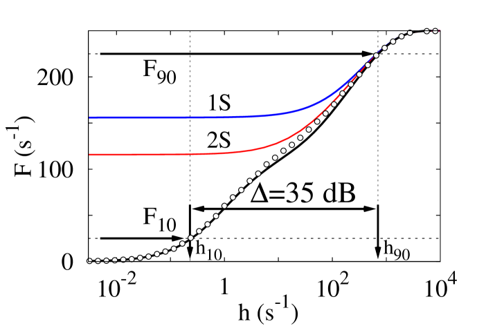
Figure 2: (Color online) Response curve $F(h)$ for simulations (symbols) and mean-field approximations (lines; 1S, 2S and black for EW) for $p_{\lambda}=0.7$ and $G=10$. Horizontal and vertical arrows show the relevant parameters for calculating the dynamic range $\Delta$ (see Eq. 1).

Several features of this model have been explored previously (Gollo et al., 2009), like the dependence of $\Delta$ on model parameters, the double-sigmoid character of the response function, as well as the robustness of the results with respect to variants which increase biological plausibility. All these were based on simulations only. We now attempt to reproduce the results analytically.

III Mean-Field Approximations

III.1 Master equation

The system can be formally described by a set of master equations. For the general case of arbitrary $k$, let $P_{t}^{g}\left(x;y;u^{(i)},v^{(j)},\ldots\right)$ be the joint probability that at time $t$ a site at generation $g$ is in state $y$, its mother site at generation $g-1$ is in state $x$, $i$ ($j$) of its daughter branches at generation $g+1$ are in state $u$ ($v$) etc.

Although the results in this paper are restricted to trees with $k=2$, for completeness we write down the master equation for general $k$. The explicit derivation of the master equations for any layer is shown in Appendix A. The equations for $0<g<G$ can be written as follows:

$$P_{t+1}^{g}(;1;) = P_{t}^{g}(;0;)-\left(1-p_{h}\right)\sum^{k}_{i=0}\biggl{[}p_{\lambda}^{i}{k\choose i}(-1)^{i}P_{t}^{g}\left(;0;1^{(i)}\right)$$ (2)

$$-\beta p^{i+1}_{\lambda}{k\choose i}(-1)^{i}P_{t}^{g}\left(1;0;1^{(i)}\right)\biggr{]}+(1-p_{\delta})P_{t}^{g}(;1;)\;,$$

$$P_{t+1}^{g}(;2;) = p_{\delta}P_{t}^{g}(;1;)+(1-p_{\gamma})P_{t}^{g}(;2;)\;,$$ (3)

$$P_{t+1}^{g}(;0;) = 1-P_{t+1}^{g}(;1;)-P_{t+1}^{g}(;2;)\;,$$ (4)

where $P_{t}^{g}(x;y;w^{(0)})\equiv P_{t}^{g}(x;y;)$ is a two-site joint probability and $P_{t}^{g}(;y;)$ [also written $P_{t}^{g}(y)$ for simplicity] is the probability of finding at time $t$ a site at generation $g$ in state $y$ (regardless of its neighbors).

Equations for the central ($g=0$) and border ($g=G$) sites can be obtained from straightforward modifications of Eq. 2, rendering

$$P_{t+1}^{0}(;1;) = P_{t}^{0}(;0;)-\left(1-p_{h}\right)\sum^{k+1}_{i=0}\biggl{[}p_{\lambda}^{i}{k+1\choose i}(-1)^{i}P_{t}^{0}\left(;0;1^{(i)}\right)\biggr{]}$$ (5)

$$+(1-p_{\delta})P_{t}^{0}(;1;)\;,$$

$$P_{t+1}^{G}(;1;) = P_{t}^{G}(;0;)+(1-p_{h})\left[\beta p_{\lambda}P^{G}_{t}(1;0;)\right]+(1-p_{\delta})P_{t}^{G}(;1;)\;,$$ (6)

whereas Eqs. 3 and 4 remain unchanged. Naturally, the full description of the dynamics would require higher-order terms (infinitely many in the limit $G\to\infty$), but Eqs 2 to 4 suffice to yield the mean-field equations we address below.

III.2 Single-site mean-field approximation

The simplest method for truncating the master equations is the standard single-site (1S) mean-field approximation (Marro and Dickman, 1999), which results from discarding the influence of any neighbors in the conditional probabilities: $P_{t}^{g}(y|x)\equiv P_{t}^{g}(;y;x)/P_{t}^{g+1}(;x;)\stackrel{{\scriptstyle(1S)}}{{\approx}}P_{t}^{g}(y)$. If this procedure is applied separately for each generation $g$, one obtains the factorization $P_{t}^{g}\left(x;y;u^{(i)},v^{(j)}\right)\stackrel{{\scriptstyle(1S)}}{{\approx}}P_{t}^{g-1}(x)P_{t}^{g}(y)[P_{t}^{g+1}(u)]^{i}[P_{t}^{g+1}(v)]^{j}$, which reduces the original problem to a set of coupled equations for single-site probabilities:

$$P^{g}_{t+1}(1) \stackrel{{\scriptstyle(1S)}}{{\simeq}} P^{g}_{t}(0)\Lambda^{g}(t)+(1-p_{\delta})P_{t}^{g}(1)\;,$$ (7)

where

$$\Lambda^{g}(t)=1-(1-p_{h})\left[1-\beta p_{\lambda}P^{g-1}_{t}(1)\right]\left[1-p_{\lambda}P^{g+1}_{t}(1)\right]^{k}$$ (8)

is the probability of a quiescent site becoming excited due to either an external stimulus or propagation from at least one of its $z=k+1$ neighbors (i.e., for $0<g<G$). For $g=0$ and $g=G$ one has

$$\Lambda^{0}(t) = 1-(1-p_{h})\left[1-p_{\lambda}P^{1}_{t}(1)\right]^{k+1}\;,$$ (9)

$$\Lambda^{G}(t) = 1-(1-p_{h})\left[1-\beta p_{\lambda}P^{G-1}_{t}(1)\right]\;.$$ (10)

Note that this approximation retains some spatial information through its index $g$, whereby the generation-averaged activation $P_{t}^{g}(1)$ is coupled to $P_{t}^{g+1}(1)$ and $P_{t}^{g-1}(1)$, rendering a $2(G+1)$-dimensional map as the reduced dynamics [note that the dimensionality of the probability vector is $3(G+1)$, but normalization as in Eq. 4 reduces it to $2(G+1)$]. Although this facilitates the incorporation of finite-size effects (which are necessary for comparison with finite-$G$ system simulations), we will see below that the results are not satisfactory. In fact, the results are essentially unchanged if we further collapse the different generations: $P_{t}^{g}(x)=P_{t}(x)$, $\forall g$ (which is the usual mean-field approximation, implying surface terms are to be neglected in the limit $G\to\infty$). The reasons for keeping a generation dependence will become clear when we propose a different approximation (see section III.4).

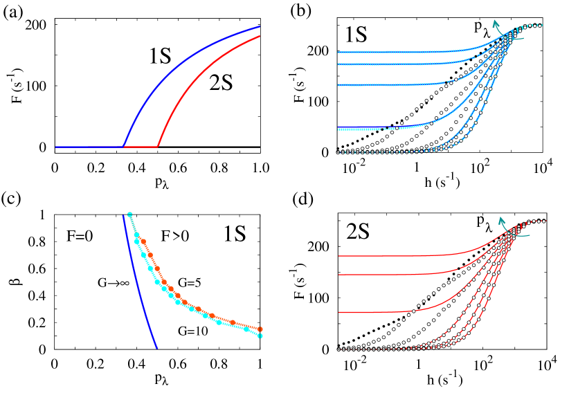
Figure 3: (Color online) Mean-field approximations. (a) Firing rate of the 1S, 2S and EW (black) approximations in the absence of stimulus ($h=0$). (b) Family of response functions for $\beta=1$ and $p_{\lambda}=0,0.2,0.4,\ldots,1$. Symbols represent simulations (as in Ref. Gollo et al. (2009)) and curves are the 1S mean-field approximation. Open (closed) symbols correspond to probabilistic (deterministic, $p_{\lambda}=1$) neighbor coupling, and dotted (continuous) curves correspond to $G=10$ ($G\to\infty$). (c) Phase diagram under the 1S approximation for different system sizes. (d) Same as (b) but for 2S approximation with $G\to\infty$.

To compare our results with the case of interest for real dendrites, in the following we restrict ourselves to the binary tree, namely $k=2$. Figure 3(a) shows the results for the stationary value $F\equiv\frac{1}{\Delta t}\lim_{t\to\infty}P_{t}^{0}(1)$ in the absence of stimulus, i.e., the fixed point of the 1S mean-field equations for $h=0$, as a function of the branchlet coupling $p_{\lambda}$. The parameter values are $G=10$, $\beta=1$ and $p_{\delta}=1$ (deterministic spike duration). In the absence of stimulus, we see that the 1S approximation predicts a phase transition at $p_{\lambda}=p_{\lambda c}^{(1S)}=1/3$. As a consequence, the response curve $F(h)$ for $p>p_{\lambda c}^{(1S)}$ displays a plateau in the limit $h\to 0$, as shown in Fig. 3(b). The 1S approximation yields results comparable to simulations only below $p_{\lambda c}^{(1S)}$, but performs rather poorly above the phase transition it predicts. However, given the deterministic spike duration (the only state in which a given site can excite its neighbors) and the absence of loops in the topology, a stable phase with stable self-sustained activity cannot exist (Furtado and Copelli, 2006; Gollo et al., 2009).

Figure 3(b) also shows the response curves as predicted by the simplified equations obtained from the $G\to\infty$ limit [i.e., by collapsing all layers, $P_{t}^{g}(x)=P_{t}(x)$, $\forall g$]. Since they nearly coincide with the equations for $G=10$ (which have a much higher dimensionality), it suffices to work with $G\to\infty$, which lends itself to analytical calculations. By expanding (around $F\simeq 0$) the single equation resulting from Eqs. 3, 4, 7 and 8 in their stationary states, one obtains the value of critical value of $p_{\lambda}$ as predicted by the 1S approximation for general $k$, $p_{\delta}$ and $\beta$:

$$p^{(1S)}_{\lambda c}=\frac{p_{\delta}}{k+\beta}\;.$$ (11)

Still with $p_{h}=0$ [i.e., in the absence of stimulus ($h=0$)], and recalling that $\Delta t=1$ ms (i.e., rates $F$ and $h$ are expressed in kHz), the 1S approximation yields the following behavior near criticality (i.e., for $p_{\lambda}\gtrsim p^{(1S)}_{\lambda c}$):

$$F(h=0,\epsilon)\simeq\frac{p_{\delta}}{C}{\epsilon}^{\tilde{\beta}}\;,$$ (12)

where $\tilde{\beta}=1$ is a critical exponent, $\epsilon=\frac{p_{\lambda}-p^{(1S)}_{\lambda c}}{p^{(1S)}_{\lambda c}}$, and $C=\frac{kp_{\delta}^{2}}{(k+\beta)^{2}}\left[\frac{(k-1)}{2}+\beta\right]+\frac{p_{\gamma}+p_{\delta}}{p_{\gamma}}$. Since in this case the order parameter corresponds to a density of activations and the system has no symmetry or conserved quantities, $\tilde{\beta}$ corresponds to the mean-field exponent of systems belonging to the directed percolation (DP) universality class (Marro and Dickman, 1999).

The response function can also be obtained analytically for weak stimuli (for $h\ll\epsilon$, $p_{h}\ll 1$, thus $p_{h}\simeq h\Delta t=h$). Below criticality ($p_{\lambda}<p^{(1S)}_{\lambda c}$), the response is linear:

$$F(h,\epsilon)\simeq\frac{h}{p_{\delta}|\epsilon|}\;.$$ (13)

As is usual in these cases, the linear response approximation breaks down at $p_{\lambda}=p^{(1S)}_{\lambda c}$ (Furtado and Copelli, 2006). For $p_{\lambda}=p^{(1S)}_{\lambda c}$, one obtains instead

$$F(h,\epsilon=0)\simeq\left(\frac{h}{C}\right)^{1/\delta_{h}}\;,$$ (14)

where $\delta_{h}=2$ is again a mean-field exponent corresponding to the response at criticality (Marro and Dickman, 1999).

In Fig. 3(c) we show in the plane $(p_{\lambda},\beta)$ the critical line given by Eq. 11, as well as the line obtained by numerically iterating Eqs. 7-10 for finite $G$. It is interesting to note that the curves for $G\to\infty$ and $G=5,10$ split when $\beta$ decreases. If one remembers that the simulated model has no active phase, the resulting phase diagram suggests that the 1S solution can perform well for $\beta\simeq 0$. Unfortunately, however, the limit $\beta\to 0$ corresponds to the absence of backpropagating spikes, which in several cases of interest is far from a realistic assumption (backpropagation of action potentials well into the dendritic tree has been observed experimentally (Johnston et al., 1996; Stuart and Sakmann, 1994)).

III.3 Two-site mean-field approximation

The next natural step would be to consider the so-called pair or two-site (2S) mean-field approximation (Marro and Dickman, 1999), in which only nearest-neighbor correlations are kept: $P_{t}(x|y,u,v)\stackrel{{\scriptstyle(2S)}}{{\approx}}P_{t}(x|y)$. In that case, the dynamics of one-site probabilities end up depending also on two-site probabilities (Furtado and Copelli, 2006). Those, on their turn, depend on higher-order terms, but under the 2S truncation these can be approximately written in terms of one-site and two-site probabilities. The schematic representation of a general pair of neighbor sites ($x$ and $y$), along with their corresponding neighbors ($a$, $b$ and $u$, $v$), is depicted in Fig 4. In the case of an infinite tree, and restraining oneself to the isotropic case $\beta=1$, one can drop the generation index $g$ and employ the isotropy assumption $P_{t}(x,y)=P_{t}(y,x)$ to write the general joint probability in the two-site approximation as

$$P_{t}(a;x;y,b;u,v)\stackrel{{\scriptstyle(2S)}}{{\approx}}\frac{P_{t}(a;x)P_{t}(x;b)P_{t}(x;y)P_{t}(y;u)P_{t}(y;v)}{[P_{t}(x)P_{t}(y)]^{2}}\;.$$ (15)

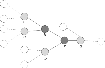
Figure 4: Two-site mean-field approximation schematic representation of a general pair ($x$ and $y$) in a binary tree ($k=2$). In order to describe the dynamics of $x$ and $y$, each of their neighbors must be taken into account. According to Eq. 15, the joint probability of the labeled sites is rewritten in terms of two-site probabilities.

In this simplified scenario, the collective dynamics is reduced to that of a probability vector containing two-site probabilities (from which single-site probabilities can be obtained, please refer to Appendix B). Taking all normalizations into account, the dimensionality of this vector can be reduced to 5. As can be seen in Appendix B, however, this simple refinement in the mean-field approximation already leads to very cumbersome equations.

As shown in Figs. 2, 3(a), and 3(d), the gain in the quality of the approximation falls far short of the increase in the complexity of the calculations. In fact, the 1S and 2S approximations yield qualitatively similar results, capturing the essential features of the system behavior only for $p_{\lambda}$ smaller than some critical value $p_{\lambda c}$. For $p_{\lambda}>p_{\lambda c}$, both approximations predict a phase transition to self-sustained activity, with $p_{\lambda c}=1/3$ for 1S and $p_{\lambda c}=1/2$ for 2S (in the case $\beta=1=p_{\delta}$). These predictions are incorrect: when simulating the model without external driving ($h=0$), in a few time steps [${\cal O}(G)$] the system goes to an absorbing state (Marro and Dickman, 1999), from which it cannot scape in the absence of further stimulation.

One can interpret the results of the approximations as follows. At the 1S approximation level, a quiescent site will typically be activated by any of its three spiking neighbors at the phase transition, hence $p_{\lambda c}=1/3$. The refinement of the 2S approximation consists in keeping track of the excitable wave propagation from one neighbor, leaving two other neighbors (wrongly assumed to be uncorrelated) available for activity propagation, hence $p_{\lambda c}=1/2$.

One could, in principle, attempt to solve this problem by increasing the order of the cluster approximation (keeping, e.g., 3- and 4-site terms). However, the resulting equations are so complicated that their usefulness would be disputable, especially for applications in Neuroscience. It is unclear how more sophisticated mean-field approaches (such as, e.g., non-equilibrium cavity methods (Mezard et al., 1987; Skantzos et al., 2005; Hatchett and Uezu, 2008)) would perform in this system. In principle, they seem particularly appealing to deal with the case $p_{\delta}<1$, when a phase transition to an active state is allowed to occur (and whose universality class is expected to coincide with that of the contact process on trees (Pemantle, 1992; Morrow et al., 1994)). Attempts in this direction are promising and would be welcome.

In the following section, we propose an alternative approximation scheme which circumvents the difficulties of the regime $p_{\lambda}\lesssim 1$ and at the same time takes into account finite-size effects.

III.4 Excitable-wave mean-field approximation

The difficulties of the 1S and 2S approximations with the strong-coupling regime are not surprising. Note that the limit of deterministic propagation (approached in our model as $p_{\lambda}\to 1$) of deterministic excitations ($p_{\delta}=1$) is hardly handled by continuous-time Markov processes on the lattice. To the best of our knowledge, a successful attempt to analytically determine the scaling of the response function to a Poisson stimulus of a hypercubic deterministic excitable lattice was published only recently (Ohta and Yoshimura, 2005) (and later confirmed in biophysically more detailed models (Ribeiro and Copelli, 2008)). While these scaling arguments have not yet been adapted to the Cayley tree, the collective response resulting from the interplay between the propagation and annihilation of quasi-deterministic excitable waves remains an open and important problem. In the following, we restricy ourselves to the case $p_{\delta}=1$, i.e., deterministic spike duration.

As discussed above, the 1S and 2S approximations give poor results essentially because they fail to keep track of where the activity reaching a given site comes from. We therefore propose here an excitable-wave (EW) mean-field approximation which attempts to address precisely this point.

The rationale is simple: in an excitable tree, activity can always be decomposed in forward- and backward-propagating excitable waves. Formally, this is implemented as follows. We separate (for $g>0$) the active state (1) into three different active states: 1A, 1B, and 1C, as represented in Fig. 5(a). $P_{t}^{g}(1A)$ stands for the probability that activation (at layer $g$ and time $t$) was due to the input received from an external source (controlled by $p_{h}$). The density of elements in 1A can excite quiescent neighbors at both the previous and the next layers. $P_{t}^{g}(1B)$ corresponds to the density of elements in layer $g$ which were quiescent at time $t-1$ and received input from the next layer ($g+1$) (i.e., a forward propagation). The density of elements in 1B can excite solely quiescent neighbors at the previous layer. Finally, $P_{t}^{g}(1C)$ accounts for the activity coming from the previous layer (i.e., backpropagation). The density of elements in 1C can excite solely quiescent neighbors at the next layer. For lack of a better name, we refer to these different virtual states as excitation components. Figure 5(b) represents the activity flux in the dendritic tree as projected by the EW mean-field approximation. The absence of loops guarantees the suppression of the spurious non-equilibrium phase transition predicted by the traditional cluster expansions.

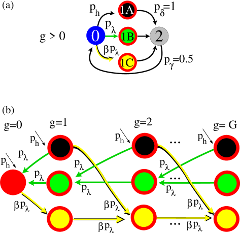
Figure 5: (Color online) Schematic representation of the excitable-wave mean-field approximation. (a) Dynamics of each layer ($g>0$) in the excitable-wave (EW) mean-field approximation (see text for details). There are 3 different active states: 1A represents activity coming from an external input; 1B is reached due to forward activity from the next layer, whereas 1C is excited by backpropagating activity from the previous layer. (b) Schematic EW mean-field approximation dynamics in a tree with $G$ layers. Note that there are no loops in the activity flux.

Following these ideas, one can write the equations for the $g>0$ layers as

$$P^{g}_{t+1}(1A) = P^{g}_{t}(0)\Lambda^{g}_{A}\;,$$ (16)

$$P^{g}_{t+1}(1B) = P^{g}_{t}(0)(1-\Lambda^{g}_{A})\Lambda^{g}_{B}(t)\;,$$ (17)

$$P^{g}_{t+1}(1C) = P^{g}_{t}(0)(1-\Lambda^{g}_{A})\left[1-\Lambda^{g}_{B}(t)\right]\Lambda^{g}_{C}(t)\;,$$ (18)

where, in analogy with Eq. 8, the excitation probabilities are now given by

$$\Lambda^{g}_{A} = p_{h},$$ (19)

$$\Lambda^{g}_{B}(t) = 1-\left\{1-p_{\lambda}\left[P^{g+1}_{t}(1A)+P^{g+1}_{t}(1B)\right]\right\}^{k},$$ (20)

$$\Lambda^{g}_{C}(t) = \beta p_{\lambda}\left[P^{g-1}_{t}(1A)+P^{g-1}_{t}(1C)\right].$$ (21)

Equations 3 and 4 remain unchanged, with $P^{g}_{t}(1)\equiv P^{g}_{t}(1A)+P^{g}_{t}(1B)+P^{g}_{t}(1C)$. The dynamics of the most distal layer $g=G$ is obtained by fixing $\Lambda_{B}^{G}(t)=0$. The apical ($g=0$) element has a simpler dynamics since it does not receive backpropagating waves, so its activity is governed by Eq. 7, with $g=0$ and $\Lambda^{0}(t)=1-(1-p_{h})\left\{1-p_{\lambda}\left[P^{1}_{t}(1A)+P^{1}_{t}(1B)\right]\right\}^{k+1}$ instead of Eq. 8. Taking into account the normalization conditions, the dimensionality of the map resulting from the EW approximation is $4(G-1)+5$.

It is important to notice that, while Eqs. 19-21 are relatively straightforward, there is a degree of arbitrariness in the choice of Eqs. 16-18. As written, they prescribe an ad hoc priority order for the recruitment of the excitation components of the EW equations: first by synaptic stimuli (Eq. 16), then by forward propagating waves (Eq. 17), and finally by backpropagating waves (Eq. 18). This choice seems to be appropriate in the regime of weak external driving, insofar as the order coincides with that of the events observed in the experiments: forward dendritic spikes, a somatic spike, then backpropagating dendritic spikes (Stuart and Sakmann, 1994). Appendix C compares the response functions for different priority orders to emphasize the robustness of the approximation with respect to that.

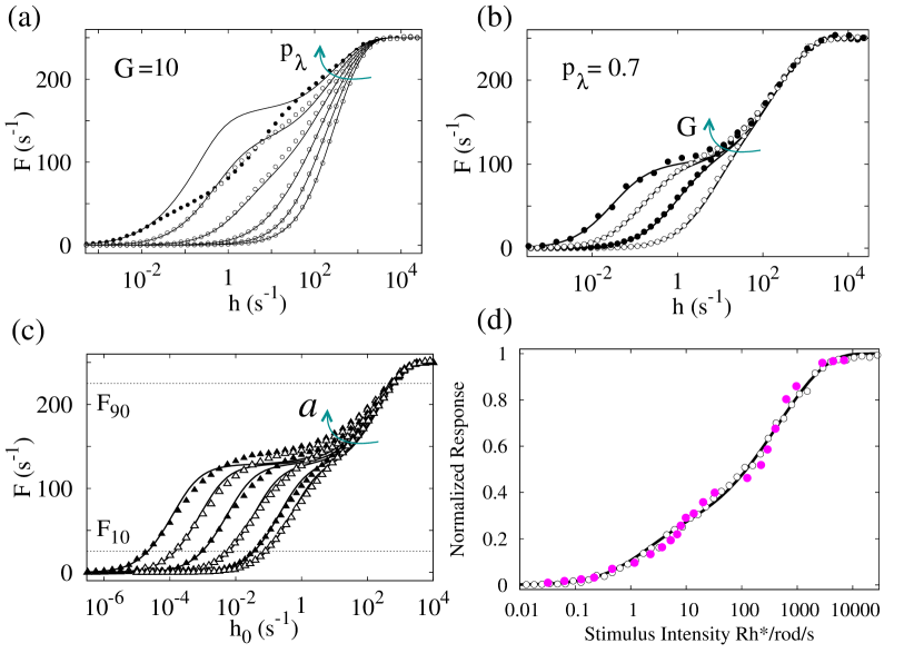
Figure 6: (Color online) Response functions: simulations compared to the EW approximation (both with $\beta=1$) and experimental data. (a) Family of response functions for $G=10$ and $p_{\lambda}=0,0.2,0.4,\ldots,1$. Symbols are the simulations (as in Ref. Gollo et al. (2009)) and solid curves are the EW mean-field approximation. (b) Family of response functions for $p_{\lambda}=0.7$ and different tree sizes: $G=5,10,15,20$. (c) Simulations and EW response function for external stimuli spatially distributed as $h(g)=h_{0}e^{ag}$: from right to left, $a=0,0.1,0.3,\ldots,0.9$ ($p_{\lambda}=0.8$ and $G=10$). Horizontal lines are plotted for the estimation of the dynamic range. (d) Experimental result from mouse retinal ganglion cells shows double sigmoid response curves (closed symbols) as a function of stimulus $I$ (measured in rhodopsins/isomerizations/rod/second (Deans et al., 2002)). They can be reasonably well fit by both simulations (open symbols, $p_{\lambda}=0.58$ and $h=0.37$ I) and the EW response function ($p_{\lambda}=0.59$ and $h=0.4$ I) with tree size $G=15$.

Though noncontrolled, the EW mean-field approximation does provide excellent agreement with simulations. The results for $G=10$ can be seen in Fig. 6(a), which shows a family of response curves $F(h)$ for varying coupling $p_{\lambda}$. One observes that the EW mean-field results (lines) follow the simulation results (symbols) very closely up to $p_{\lambda}\simeq 0.8$, reproducing even the double-sigmoidal behavior of the curves (Deans et al., 2002; Gollo et al., 2009; Ferrante et al., 2009; Jedlicka et al., 2010). For larger values of $p_{\lambda}$, agreement is restricted to very small or very large values of $h$ (for intermediate values of $h$, note that $F(p_{\lambda})$ is nonmonotonous, a rather counterintuitive phenomenon called “screening resonance” (Gollo et al., 2009)). Most importantly, however, the EW equations eliminate the phase transition wrongly predicted by the traditional mean-field approximations.

In a real neuron, the number of layers is finite [${\cal O}(10)$ or less] and it would be extremely interesting to have an analytical approximation which managed to take finite-size effects into account. As it turns out, the mean-field approximation we propose can do precisely that, since it couples densities at different layers (so $G$ again controls the dimensionality of the mean-field map). Figure 6(b) compares simulations (symbols) with the stationary state of the EW mean-field equations (lines) for different system sizes. Note that the agreement is excellent from $G=5$ up to $G=20$, for the whole range of $h$ values.

The EW mean-field approximation is also very robust against previously proposed variants of the model. For instance, in several neurons the distribution of synaptic inputs along the dendritic tree is nonuniform, increasing with the distance from the soma. A one-parameter variant which incorporates this nonuniformity consists in a layer-dependent rate $h(g)=h_{0}e^{ag}$ (Gollo et al., 2009), as described in section II. Figure 6(c) depicts a good agreement between simulations and the EW approximation for a range of $a$ values.

Also shown in Fig. 6(d) is a comparison among experimental results from retinal ganglion cells to varying light intensity (Deans et al., 2002) (closed symbols), simulations (open symbols), and EW mean-field approximation (lines), which agree reasonably well. Therefore the approximation we propose can, in principle, be useful for fitting experimental data and reverse-engineering parameter values from data-based response functions at a relatively small computational cost (say, compared to simulations). In this particular example, it is important to emphasize that the experimental response curves are, in principle, influenced by other retinal elements. Given the very simple nature of our model, it is hard to pinpoint which part of the retinal circuit our Cayley tree would represent. Following Shepherd Shepherd (1998); Gollo et al. (2009), however, we suggest that the ganglionar dendritic arbor plus the retinal cells connected to it by gap junctions (electrical synapses) can be viewed as an extended active tree similar to the one studied here, with a large effective $G$.

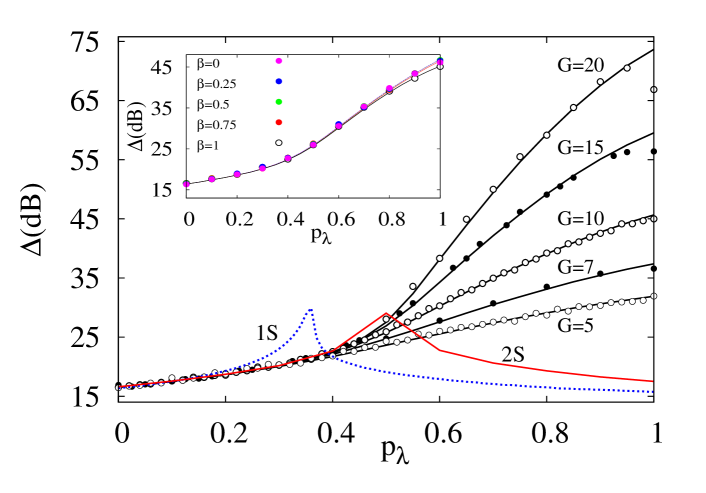
Figure 7: (Color online) Dynamic range as a function of the coupling parameter for 1S ($G=10$), 2S (infinite tree), EW (black lines) mean-field approximations compared to simulations (symbols, as in Ref. Gollo et al. (2009)) for different trees sizes $G$. The inset shows the dynamic range of dendritic trees subjected to an asymmetrical activity propagation probability controlled by $\beta$ (symbols stand for the simulations and the curves for the EW approximation for $G=10$).

The dynamic range $\Delta$ is one of the features of the response function which has received attention in the literature in recent years (Copelli et al., 2002, 2005; Copelli and Kinouchi, 2005; Furtado and Copelli, 2006; Kinouchi and Copelli, 2006; Copelli and Campos, 2007; Wu et al., 2007; Assis and Copelli, 2008; Ribeiro and Copelli, 2008; Publio et al., 2009; Shew et al., 2009; Larremore et al., 2011a, b; Buckley and Nowotny, 2011). Here it serves the purpose of summarizing the quality of the EW mean-field approximation in comparison with model simulations. In Fig. 7 we plot $\Delta$ as a function of $p_{\lambda}$ for several system sizes $G$. Both the 1S and 2S mean-field approximations predict a non-equilibrium phase transition in the model, where a peak of the dynamic range therefore occurs (Kinouchi and Copelli, 2006). Both approximations perform badly especially in the high-coupling regime. The EW approximation correctly predicts the overall behavior of the $\Delta(p_{\lambda})$ curves, for all system sizes we have been able to simulate. Finally, the inset of Fig. 7 shows a second variant of the model in which the parameter $\beta$, which controls the probability of a spike backpropagating, is free to change. Once more, the EW approximation manages to reproduce the $\Delta(p_{\lambda})$ curves obtained from simulations for the full range of $\beta$ values.

IV Conclusions

The need for a theoretical framework to deal with active dendrites has been largely recognized. However, the plethora of physiological details which are usually taken into account to explain local phenomena renders the problem of understanding the dynamics of the tree as a whole analytically untreatable. What we have proposed is the use of a minimalist statistical physics model in which our ignorance about several physiological parameters is thrown into a single parameter $p_{\lambda}$. The model has provided several insights and predictions, most of them yet to be tested experimentally (Gollo et al., 2009). Here we have shown that the model is amenable to analytical treatment as well.

We have compared different mean-field solutions to the model, and shown that standard cluster approximations (1S and 2S) yield poor results. They incorrectly predict phase transitions which are not allowed in the model, thereby failing to reproduce the response functions precisely in the low-stimulus and highly nonlinear regime (where most of the controversies are bound to arise (Bhandawat et al., 2007)).

To overcome this scenario we developed an excitable-wave mean-field approximation which takes into account the direction in which the activity is propagating through the different layers of the tree. Though ad hoc, the approximation reproduces simulation results with very reasonable accuracy, for a wide range of parameters and two biologically relevant variants of the model. We hope that our EW mean-field approximation may therefore contribute to the theoretical foundation of dendritic computation (Abbott, 2008).

It is important to recall that the theory attempts to address a model in a regime which is expected to be close to that of a neuron in vivo: dendritic spikes are generated at random, may or may not propagate along the dendrites, and annihilate each other upon collision. Our model allows one to formulate theoretical predictions for in vivo experiments in sensory system neurons, e.g., ganglion cells (Deans et al., 2002), olfactory mitral cells (Wachowiak and Cohen, 2001) or their insect counterparts, i.e., antennal lobe projection neurons (Bhandawat et al., 2007): a) if one removes part of the dendritic tree and/or b) blocks the ionic channels responsible for dendritic excitability, one should see a decrease in the neuronal dynamic range. To the best of our knowledge, these experiments have not been done yet.

Another issue upon which our results could have a bearing is the so-called gain control modulation. In the neuroscience literature, the term refers to the neuronal capacity to change the slope of the input-output response function (Rothman et al., 2009). This property has been reported in visual (Tovee et al., 1994; Brotchie et al., 1995; Treue and Trujillo, 1999; Anderson et al., 2000), somatosensory (Yakusheva et al., 2007) and auditory (Ingham and McAlpine, 2005) systems. Several possible mechanisms have already been proposed to explain gain control, based on synaptic depression (Abbott et al., 1997; Rothman et al., 2009), background synaptic input (Chance et al., 2002; Fellous et al., 2003), noise (Hansel and van Vreeswijk, 2002), shunting inhibition (Mitchell and Silver, 2003; Prescott and De Koninck, 2003) and excitatory (NMDA (Berends et al., 2005)) as well as inhibitory (GABA_A (Semyanov et al., 2004)) ionotropic receptor dynamics.

All these mechanisms are intercellular, in the sense that they rely on the influence of factors external to the neuron. Our model, on the other hand, shows gain control in its dependence on the coupling parameter $p_{\lambda}$, which controls the propagation of dendritic spikes within the tree. It is therefore an intracellular mechanism which offers an additional explanation for this ubiquitous phenomenon.

The physics of complex systems is becoming more and more embracing, shedding light in different areas, including neuroscience. Particularly at the cellular and subcellular levels, we foresee the merging of the two fields, dendritic computation and statistical physics, as a promising avenue. The maturity of the latter could illuminate several frontiers in neuroscience.

V Acknowledgments

The authors acknowledge financial support from the Brazilian agency CNPq. LLG and MC have also been supported by FACEPE, CAPES and special programs PRONEX. MC has received support from PRONEM and INCeMaq. This research was also supported by a grant from the MEC (Spain) and FEDER under project FIS2007-60327 (FISICOS) to LLG. LLG is appreciative to Prof. John Rinzel and his working group for the hospitality and valuable discussions during his 3-month visit, March to May, 2009 in the Center for Neural Science at New York University.

Appendix A Derivation of the general master equation

Let us illustrate how the master equation is obtained by starting with the simplest possible case, namely, the latest layer of the Cayley tree. Sites at the surface connect to a single site (their mother branchlet), so the probability of their being excited at time $t+1$ is

$$P_{t+1}^{G}(;1;)=[1-(1-p_{h})(1-\beta p_{\lambda})]P_{t}^{G}(1;0;)+p_{h}\sum_{l\neq 1}P_{t}^{G}(l;0;)+(1-p_{\delta})P_{t}^{G}(;1;)\;.$$ (22)

Each term has a straightforward interpretation: the first term corresponds to the probability that the surface site is quiescent (state 0), its neighbor is active (state 1), and excitation gets to the surface via an external stimulus ($p_{h}$) and/or backpropagating transmission ($\beta p_{\lambda}$); the second term corresponds to the excitation of the surface site via an external stimulus, provided that it is quiescent (0) and its neighbor is in any state other than active (1); the third term corresponds to the probability that the surface site was in state 1 and did not move to state 2 (a transition controlled by $p_{\delta}$, see Fig. 1c).

The next easiest case to consider is that of the root ($g=0$) site. It connects to $k+1$ daughter branchlets, and can be excited by any number of them. Contrary to the $g=G$ surface sites, the root site only receives forward propagating activity (hence $\beta$ plays no role). Analogously to Eq. 22, the equation for $P_{t+1}^{0}$ is given by

$$P_{t+1}^{\,0}(;1;) = \left[1-(1-p_{h})(1-p_{\lambda})^{k+1}\right]P_{t}^{\,0}(;0;1^{(k+1)}){k+1\choose k+1}$$ (23)

$$+\left[1-(1-p_{h})(1-p_{\lambda})^{k}\right]\sum_{j_{1}\neq 1}P_{t}^{\,0}(;0;1^{(k)},j_{1}){k+1\choose k}$$

$$+\left[1-(1-p_{h})(1-p_{\lambda})^{k-1}\right]\sum_{j_{1},j_{2}\neq 1}P_{t}^{\,0}(;0;1^{(k-1)},j_{1},j_{2}){k+1\choose k-1}$$

$$+\;\cdots\;$$

$$+\left[1-(1-p_{h})(1-p_{\lambda})^{m}\right]\sum_{j_{1},j_{2},\ldots,j_{k+1-m}\neq 1}P_{t}^{\,0}(;0;1^{(m)},j_{1},j_{2},\ldots,j_{k+1-m}){k+1\choose m}$$

$$+\;\cdots\;$$

$$+\left[1-(1-p_{h})(1-p_{\lambda})\right]\sum_{j_{1},\ldots,j_{k}\neq 1}P_{t}^{\,0}(;0;1,j_{1},\ldots,j_{k}){k+1\choose 1}$$

$$+p_{h}\sum_{j_{1},\ldots,j_{k+1}\neq 1}P_{t}^{\,0}(;0;j_{1},\ldots,j_{k+1})$$

$$+(1-p_{\delta})P_{t}^{\,0}(;1;)\;.$$

The terms of the kind $\left[1-(1-p_{h})(1-p_{\lambda})^{m}\right]$ account for the excitation of the root site via an external stimulus and/or via transmission from $m$ of its active daughter branchlets, regardless of the state of its $k+1-m$ non-active neighbors (hence the sum over $j_{1},j_{2},\ldots,j_{k+1-m}\neq 1$). Each term is weighted by the number ${k+1\choose m}$ of combinations of $m$ active sites out of $k+1$. The sum of these terms (from $m=1$ to $m=k+1$) therefore plays a role equivalent to that of the first term in eq. 22. The two last terms are analogous to those of eq. 22.

Finally, we come to the equation for a general site with $1\leq g\leq G-1$, which can be excited by both its mother as well as its daughter branchlets. The equation for $P_{t+1}^{g}$ thus generalizes the terms of the preceding equations:

$$P_{t+1}^{g}(;1;) = \left[1-(1-p_{h})(1-\beta p_{\lambda})(1-p_{\lambda})^{k}\right]P_{t}^{g}(1;0;1^{(k)}){k\choose k}$$ (24)

$$+\left[1-(1-p_{h})(1-\beta p_{\lambda})(1-p_{\lambda})^{k-1}\right]\sum_{j_{1}\neq 1}P_{t}^{g}(1;0;1^{(k-1)},j_{1}){k\choose k-1}$$

$$+\;\cdots\;$$

$$+\left[1-(1-p_{h})(1-\beta p_{\lambda})(1-p_{\lambda})\right]\sum_{j_{1},\ldots,j_{k-1}\neq 1}P_{t}^{g}(1;0;1,j_{1},\ldots,j_{k-1}){k\choose 1}$$

$$+\left[1-(1-p_{h})(1-\beta p_{\lambda})\right]\sum_{j_{1},\ldots,j_{k}\neq 1}P_{t}^{g}(1;0;j_{1},\ldots,j_{k}){k\choose 0}$$

$$+\left[1-(1-p_{h})(1-p_{\lambda})^{k}\right]\sum_{\ell\neq 1}P_{t}^{g}(\ell;0;1^{(k)}){k\choose k}$$

$$+\left[1-(1-p_{h})(1-p_{\lambda})^{k-1}\right]\sum_{\ell,j_{1}\neq 1}P_{t}^{g}(\ell;0;1^{(k-1)},j_{1}){k\choose k-1}$$

$$+\;\cdots\;$$

$$+\left[1-(1-p_{h})(1-p_{\lambda})\right]\sum_{\ell,j_{1},\ldots,j_{k-1}\neq 1}P_{t}^{g}(\ell;0;1,j_{1},\ldots,j_{k-1}){k\choose 1}$$

$$+p_{h}\sum_{\ell,j_{1},\ldots,j_{k}\neq 1}P_{t}^{g}(\ell;0;j_{1},\ldots,j_{k}){k\choose 0}$$

$$+(1-p_{\delta})P_{t}^{g}(;1;)\;.$$

Equations 22-24 can be drastically simplified (Furtado and Copelli, 2006). Taking into account the normalization condition

$$P_{t}^{g}(a;b;j_{1},\ldots,j_{\ell-1})\equiv\sum_{j_{\ell}}P_{t}^{g}(a;b;j_{1},\ldots,j_{\ell-1},j_{\ell})\;,$$ (25)

the sums in eqs. 22-24 can be reduced. For instance,

$$\sum_{j_{1}\neq 1}P_{t}^{g}(\ell;0;1^{(k-1)},j_{1}) = \sum_{j_{1}}P_{t}^{g}(\ell;0;1^{(k-1)},j_{1})-P_{t}^{g}(\ell;0;1^{(k)})$$ (26)

$$= P_{t}^{g}(\ell;0;1^{(k-1)})-P_{t}^{g}(\ell;0;1^{(k)})\;.$$

Iterating this procedure and rearranging terms, one finally arrives at

$$P_{t+1}^{0}(;1;) = P_{t}^{0}(;0;1^{(0)})-\left(1-p_{h}\right)\left[\sum^{k+1}_{i=0}p^{i}_{\lambda}{k+1\choose i}(-1)^{i}P_{t}^{0}(;0;1^{(i)})\right]$$ (27)

$$+(1-p_{\delta})P_{t}^{0}(;1;)\;,$$

$$P_{t+1}^{g}(;1;) = P_{t}^{g}(;0;1^{(0)})-\left(1-p_{h}\right)\Biggl{[}\sum^{k}_{i=0}\biggl{(}p^{i}_{\lambda}{k\choose i}(-1)^{i}P_{t}^{g}(;0;1^{(i)})$$ (28)

$$-\beta p^{i+1}_{\lambda}{k\choose i}(-1)^{i}P_{t}^{g}(1;0;1^{(i)})\biggr{)}\Biggr{]}+(1-p_{\delta})P_{t}^{g}(;1;)\;,$$

$$P_{t+1}^{G}(;1;) = P_{t}^{G}(;0;1^{(0)})-\left(1-p_{h}\right)\left(P_{t}^{G}(;0;1^{(0)})-\beta p_{\lambda}P_{t}^{G}(1;0;1^{(0)})\right)$$ (29)

$$+(1-p_{\delta})P_{t}^{G}(;1;)\;.$$

Recalling that $P_{t}^{g}(x;y;w^{(0)})\equiv P_{t}^{g}(x;y;)$, we recover eqs. 2, 5 and 6.

Appendix B Two-site mean-field equations

For an infinite dendritic tree, the complete set of equations under the 2S approximation is given by:

$$P_{t+1}(0;0) \stackrel{{\scriptstyle(2S)}}{{\approx}} \{(1-p_{h})^{2}P_{t}(0;0)[p_{\lambda}P_{t}(0;1)-P_{t}(0)]^{4}$$ (30)

$$+2p_{\gamma}(1-p_{h})P_{t}(0;2)P_{t}(0)^{2}[p_{\lambda}P_{t}(0;1)-P_{t}(0)]^{2}$$

$$+p_{\gamma}^{2}P_{t}(2;2)P_{t}(0)^{4}\}\frac{1}{P_{t}(0)^{2}}\;;$$

$$P_{t+1}(0;1) \stackrel{{\scriptstyle(2S)}}{{\approx}} -\Bigl{(}P_{t}(0;1)P_{t}(0)^{2}\{-(1-p_{\delta})(1-p_{h})(1-p_{\lambda})[p_{\lambda}P_{t}(0;1)-P_{t}(0)]^{2}\}$$ (31)

$$+(1-p_{h})P_{t}(0;0)\{(1-p_{h})[p_{\lambda}P_{t}(0;1)-P_{t}(0)]^{4}$$

$$-P_{t}(0)^{2}[p_{\lambda}P_{t}(0;1)-P_{t}(0)]^{2}\}$$

$$+p_{\gamma}P_{t}(0;2)\{(1-p_{h})P_{t}(0)^{2}[p_{\lambda}P_{t}(0;1)-P_{t}(0)]^{2}-P_{t}(0)^{4}\}$$

$$-(1-p_{\delta})p_{\gamma}P_{t}(1;2)P_{t}(0)^{4}\Bigr{)}\frac{1}{P_{t}(0)^{4}}\;;$$

$$P_{t+1}(0;2) \stackrel{{\scriptstyle(2S)}}{{\approx}} \{(1-p_{\gamma})(1-p_{h})P_{t}(0;2)[p_{\lambda}P_{t}(0;1)-P_{t}(0)]^{2}$$ (32)

$$+p_{\delta}(1-p_{h})(1-p_{\lambda})P_{t}(0;1)[p_{\lambda}P_{t}(0;1)-P_{t}(0)]^{2}$$

$$+p_{\gamma}(1-p_{\gamma})P_{t}(2;2)P_{t}(0)^{2}$$

$$+p_{\delta}p_{\gamma}P_{t}(1;2)P_{t}(0)^{2}\}\frac{1}{P_{t}(0)^{2}}\;;$$

$$P_{t+1}(1;1) \stackrel{{\scriptstyle(2S)}}{{\approx}} \Bigl{(}(1-p_{h})P_{t}(0;0)\{(1-p_{h})[p_{\lambda}P_{t}(0;1)-P_{t}(0)]^{4}$$ (33)

$$-2P_{t}(0)^{2}[p_{\lambda}P_{t}(0;1)-P_{t}(0)]^{2}+P_{t}(0)^{4}\}$$

$$-2P_{t}(0;1)P_{t}(0)^{2}\{(1-p_{\delta})(1-p_{h})(1-p_{\lambda})[p_{\lambda}P_{t}(0;1)-P_{t}(0)]^{2}$$

$$-(1-p_{\delta})P_{t}(0)^{2}\}+(1-p_{\delta})^{2}P_{t}(1;1)P_{t}(0)^{4}\Bigr{)}\frac{1}{P_{t}(0)^{4}}\;;$$

$$P_{t+1}(1;2) \stackrel{{\scriptstyle(2S)}}{{\approx}} -\Bigl{(}P_{t}(0;2)\{(1-p_{\gamma})(1-p_{h})[p_{\lambda}P_{t}(0;1)-P_{t}(0)]^{2}-(1-p_{\gamma})P_{t}(0)^{2}\}$$ (34)

$$+p_{\delta}P_{t}(0;1)\{(1-p_{h})(1-p_{\lambda})[p_{\lambda}P_{t}(0;1)-P_{t}(0)]^{2}-P_{t}(0)^{2}\}$$

$$-p_{\delta}(1-p_{\delta})P_{t}(1;1)P_{t}(0)^{2}$$

$$-(1-p_{\delta})(1-p_{\gamma})P_{t}(1;2)P_{t}(0)^{2}\Bigr{)}\frac{1}{P_{t}(0)^{2}}\;;$$

$$P_{t+1}(2;2) \stackrel{{\scriptstyle(2S)}}{{\approx}} p_{\delta}^{2}P_{t}(1;1)+2p_{\delta}(1-p_{\gamma})P_{t}(1;2)+(1-p_{\gamma})^{2}P_{t}(2;2)\;.$$ (35)

In order to solve it numerically, by normalization we make use of:

$$P_{t}(0) = P_{t}(0;0)+P_{t}(0;1)+P_{t}(0;2)\;.$$ (36)

To compare the results with the simulations and experiments we use $F\equiv\frac{1}{\Delta t}\lim_{t\to\infty}P_{t}(1)$, where:

$$P_{t}(1) = P_{t}(0;1)+P_{t}(1;1)+P_{t}(1;2)\;.$$ (37)

Finally, by completeness, the last single-site probability can be obtained by:

$$P_{t}(2) = P_{t}(0;2)+P_{t}(1;2)+P_{t}(2;2)\;.$$ (38)

Appendix C Robustness with respect to the priority order of the excitable components

The priority order used in Eqs. 16-18 was “ABC”, i.e., first 1A, followed by 1B and then 1C. The virtual state 1B accounts for the forward-propagating excitable-wave flux whereas state 1C accounts for the backward-propagating excitable-wave flux. In order to compare all the different combinations, Fig. 8 displays families of response functions.

Intuitively, the neuronal firing rate $F$ increases as the forward-propagating excitable-wave flux grows. Summarizing the results, switching the order of 1B and 1C (lower panels in Fig. 8), we reduce the forward-propagating excitable-wave flux, and consequently, the response functions corresponding to large $p_{\lambda}$ values present a lower firing rate. Moreover, the result is virtually the same irrespective of the order in which 1A appears (compare panels horizontally in Fig. 8).

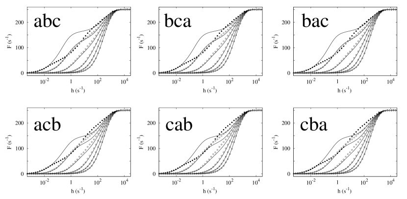
Figure 8: Effects of the priority order of the excitable components on the response functions: simulations compared to the EW approximation and experimental data. Family of response functions for $G=10$ and $p_{\lambda}=0,0.2,0.4,\ldots,1$. Top panels display combinations of 1B prior to 1C, and bottom panels the converse. Symbols are the simulations and solid curves are the EW mean-field approximation.

The approximation is robust with respect to the order chosen, and only minor differences can be found for strong coupling ($p_{\lambda}\sim 1$) and the intermediate amount of external driving input. Changes in the order of the components modify the response functions quantitatively. However, qualitatively, the response functions are very alike. Most of the differences occur at the high-coupling regime ($p_{\lambda}\sim 1$), but do not affect the localization of $h_{10}$ and $h_{90}$ (which implies that the dynamic range remains unchanged).

References

- Bower and Beeman (1995) J. M. Bower and D. Beeman, The Book of GENESIS: Exploring Realistic Neural Models with the GEneral NEural SImulation System (Springer-Verlag, 1995).
- Carnevale and Hines (2009) N. T. Carnevale and M. L. Hines, The NEURON Book (Cambridge University Press, 2009).
- Hodgkin and Huxley (1952) A. L. Hodgkin and A. F. Huxley, J. Physiol. 117, 500 (1952).
- Dayan and Abbott (2001) P. Dayan and L. F. Abbott, Theoretical Neuroscience: Computational and Mathematical Modeling of Neural Systems (MIT Press, Cambridge, Massachusetts, 2001).
- Rall (1964) W. Rall, in Neural Theory and Modeling, edited by R. F. Reiss (Stanford Univ. Press, Stanford, CA, 1964).
- Stuart et al. (2008) G. Stuart, N. Spruston, and M. Häusser, eds., Dendrites, 2nd ed. (Oxford University Press, New York, 2008).
- Koch (1999) C. Koch, Biophysics of Computation (Oxford University Press, New York, 1999).
- Eccles et al. (1958) J. C. Eccles, B. Libet, and R. R. Young, J. Physiol. 143, 11 (1958).
- Mel (1993) B. W. Mel, J. Neurophysiol. 70, 1086 (1993).
- Johnston and Narayanan (2008) D. Johnston and R. Narayanan, Trends Neurosci. 31, 309 (2008).
- Sjöström et al. (2008) P. J. Sjöström, E. A. Rancz, A. Roth, and M. Häusser, Physiol. Rev. 88, 769 (2008).
- Reyes (2001) A. Reyes, Annual Review of Neuroscience 24, 653 (2001).
- Herz et al. (2006) A. V. M. Herz, T. Gollisch, C. K. Machens, and D. Jaeger, Science 314, 80 (2006).
- London and Häusser (2005) M. London and M. Häusser, Ann. Rev. Neurosci. 28, 503 (2005).
- Poirazi and Mel (2001) P. Poirazi and B. W. Mel, Neuron 29, 779 (2001).
- Poirazi et al. (2003a) P. Poirazi, T. Brannon, and B. W. Mel, Neuron 37, 977 (2003a).
- Poirazi et al. (2003b) P. Poirazi, T. Brannon, and B. W. Mel, Neuron 37, 989 (2003b).
- Morita (2009) K. Morita, Front. Comput. Neurosci. 3, 12 (2009).
- Coop et al. (2010) A. D. Coop, H. Cornelis, and F. Santamaria, Front. Comput. Neurosci. 4, 6 (2010).
- Gollo et al. (2009) L. L. Gollo, O. Kinouchi, and M. Copelli, PLoS Comput. Biol. 5, e1000402 (2009).
- Copelli et al. (2002) M. Copelli, A. C. Roque, R. F. Oliveira, and O. Kinouchi, Phys. Rev. E 65, 060901 (2002).
- Copelli et al. (2005) M. Copelli, R. F. Oliveira, A. C. Roque, and O. Kinouchi, Neurocomputing 65-66, 691 (2005).
- Copelli and Kinouchi (2005) M. Copelli and O. Kinouchi, Physica A 349, 431 (2005).
- Furtado and Copelli (2006) L. S. Furtado and M. Copelli, Phys. Rev. E 73, 011907 (2006).
- Kinouchi and Copelli (2006) O. Kinouchi and M. Copelli, Nat. Phys. 2, 348 (2006).
- Copelli and Campos (2007) M. Copelli and P. R. A. Campos, Eur. Phys. J. B 56, 273 (2007).
- Wu et al. (2007) A.-C. Wu, X.-J. Xu, and Y.-H. Wang, Phys. Rev. E 75, 032901 (2007).
- Assis and Copelli (2008) V. R. V. Assis and M. Copelli, Phys. Rev. E 77, 011923 (2008).
- Ribeiro and Copelli (2008) T. L. Ribeiro and M. Copelli, Phys. Rev. E 77, 051911 (2008).
- Publio et al. (2009) R. Publio, R. F. Oliveira, and A. C. Roque, PLoS One 4, e6970 (2009).
- Larremore et al. (2011a) D. B. Larremore, W. L. Shew, and J. G. Restrepo, Phys. Rev. Lett. 106, 058101 (2011a).
- Larremore et al. (2011b) D. B. Larremore, W. L. Shew, E. Ott, and J. G. Restrepo, Chaos 21, 025117 (2011b).
- Buckley and Nowotny (2011) C. L. Buckley and T. Nowotny, Phys. Rev. Lett. 106, 238109 (2011).
- Kihara et al. (2009) A. H. Kihara, V. Paschon, C. M. Cardoso, G. S. V. Higa, L. M. Castro, D. E. Hamassaki, and L. R. G. Britto, J. Comp. Neurol. 512, 651 (2009).
- Shew et al. (2009) W. Shew, H. Yang, T. Petermann, R. Roy, and D. Plenz, J. Neurosci. 29, 15595 (2009).
- Lindner et al. (2004) B. Lindner, J. García-Ojalvo, A. Neiman, and L. Schimansky-Geier, Phys. Rep. 392, 321 (2004).
- Rieke et al. (1997) F. Rieke, D. Warland, R. De Ruyter Van Steveninck, and W. Bialek, Spikes: Exploring the Neural Code (MIT Press, 1997).
- Agmon-Snir et al. (1998) H. Agmon-Snir, C. E. Carr, and J. Rinzel, Nature 393, 268 (1998).
- Moser et al. (2008) E. I. Moser, E. Kropff, and M.-B. Moser, Annual Review of Neuroscience 31, 69 (2008).
- Bi and Poo (1998) G. Q. Bi and M. M. Poo, Journal of Neuroscience 18, 10464 (1998).
- Uhlhaas et al. (2009) P. J. Uhlhaas, G. Pipa, B. Lima, L. Melloni, S. Neuenschwander, D. Nikolić, and W. Singer, Frontiers in integrative neuroscience 3, 19 (2009).
- Fischer et al. (2006) I. Fischer, R. Vicente, J. M. Buldú, M. Peil, C. R. Mirasso, M. Torrent, and J. García-Ojalvo, Physical Review Letters 97, 123902 (2006).
- Vicente et al. (2008) R. Vicente, L. L. Gollo, C. R. Mirasso, I. Fischer, and G. Pipa, Proc. Natl. Acad. Sci. USA 105, 17157 (2008).
- Gollo et al. (2010) L. L. Gollo, C. Mirasso, and A. E. P. Villa, NeuroImage 52, 947 (2010).
- Gollo et al. (2011) L. L. Gollo, C. R. Mirasso, M. Atienza, M. Crespo-Garcia, and J. L. Cantero, PLoS ONE 6, 10 (2011).
- Rolls and Deco (2010) E. T. Rolls and G. Deco, The Noisy Brain: Stochastic Dynamics as a Principle of Brain Function (Oxford University Press., 2010).
- Buesing et al. (2011) L. Buesing, J. Bill, B. Nessler, and W. Maass, PLoS Comput Biol 7, e1002211 (2011).
- Rolls and Treves (2011) E. T. Rolls and A. Treves, Progress in Neurobiology 95, 1 (2011).
- Marro and Dickman (1999) J. Marro and R. Dickman, Nonequilibrium Phase Transition in Lattice Models (Cambridge University Press, Cambridge, 1999).
- Johnston et al. (1996) D. Johnston, J. C. Magee, C. M. Colbert, and B. R. Christie, Annu. Rev. Neurosci. 19, 165 (1996).
- Stuart and Sakmann (1994) G. J. Stuart and B. Sakmann, Nature 367, 69 (1994).
- Mezard et al. (1987) M. Mezard, G. Parisi, and M. Virasoro, Spin glass theory and beyond (World Scientific, Singapore, 1987).
- Skantzos et al. (2005) N. S. Skantzos, I. P. Castillo, and J. P. L. Hatchett, Phys. Rev. E 72, 066127 (2005).
- Hatchett and Uezu (2008) J. P. L. Hatchett and T. Uezu, Phys. Rev. E 78, 036106 (2008).
- Pemantle (1992) R. Pemantle, Ann. Prob. 20, 2089 (1992).
- Morrow et al. (1994) G. J. Morrow, R. B. Schinazi, and Y. Zhang, J. App. Prob. 31, 250 (1994).
- Ohta and Yoshimura (2005) T. Ohta and T. Yoshimura, Physica D 205, 189 (2005).
- Deans et al. (2002) M. R. Deans, B. Volgyi, D. A. Goodenough, S. A. Bloomfield, and D. L. Paul, Neuron 36, 703 (2002).
- Ferrante et al. (2009) M. Ferrante, M. Migliore, and G. A. Ascoli, Proc. Natl. Acad. Sci. USA 106, 18004 (2009).
- Jedlicka et al. (2010) P. Jedlicka, T. Deller, and S. W. Schcrzacher, J. Comp. Neurosci. 29, 509–19 (2010).
- Shepherd (1998) G. M. Shepherd, ed., The Synaptic Organization of the Brain, 5th ed. (Oxford University Press, New York, 1998).
- Bhandawat et al. (2007) V. Bhandawat, S. R. Olsen, N. W. Gouwens, M. L. Schlief, and R. I. Wilson, Nat. Neurosci. 10, 1474 (2007).
- Abbott (2008) L. F. Abbott, Neuron 60, 489 (2008).
- Wachowiak and Cohen (2001) M. Wachowiak and L. B. Cohen, Neuron 32, 723 (2001).
- Rothman et al. (2009) J. S. Rothman, L. Cathala, V. Steuber, and R. A. Silver, Nature 457, 1015 (2009).
- Tovee et al. (1994) M. J. Tovee, E. T. Rolls, and P. Azzopardi, J. Neurophysiol. 72, 1049 (1994).
- Brotchie et al. (1995) P. R. Brotchie, R. A. Andersen, L. H. Snyder, and S. J. Goodman, Nature 375, 232 (1995).
- Treue and Trujillo (1999) S. Treue and J. C. M. Trujillo, Nature 399, 575 (1999).
- Anderson et al. (2000) J. S. Anderson, I. Lampl, D. C. Gillespie, and D. Ferster, Science 290, 1968 (2000).
- Yakusheva et al. (2007) T. A. Yakusheva, A. G. Shaikh, A. M. Green, P. M. Blazquez, J. D. Dickman, and D. E. Angelaki, Neuron 54, 973 (2007).
- Ingham and McAlpine (2005) N. J. Ingham and D. McAlpine, J. Neurosci. 25, 6187 (2005).
- Abbott et al. (1997) L. F. Abbott, J. A. Varela, K. Sen, and S. B. Nelson, Science 275, 220 (1997).
- Chance et al. (2002) F. S. Chance, L. F. Abbott, and A. D. Reyes, Neuron 35, 773 (2002).
- Fellous et al. (2003) J. Fellous, M. Rudolph, A. Destexhe, and T. J. Sejnowski, Neurosci. 122, 811 (2003).
- Hansel and van Vreeswijk (2002) D. Hansel and C. van Vreeswijk, J. Neurosci. 22, 5118 (2002).
- Mitchell and Silver (2003) S. J. Mitchell and R. A. Silver, Neuron 38, 433 (2003).
- Prescott and De Koninck (2003) S. A. Prescott and Y. De Koninck, Proc. Natl. Acad. Sci. USA 100, 2076 (2003).
- Berends et al. (2005) M. Berends, R. Maex, and E. De Schutter, Neural Comput. 17, 2531 (2005).
- Semyanov et al. (2004) A. Semyanov, M. C. Walker, D. M. Kullmann, and R. A. Silver, Trends Neurosci. 27, 262 (2004).