Correlation length scalings in fusion
edge plasma turbulence computations

Abstract

The effect of changes in plasma parameters, that are characteristic near or at an L-H transition in fusion edge plasmas, on fluctuation correlation lengths are analysed by means of drift-Alfvén turbulence computations. Scalings by density gradient length, collisionality, plasma beta, and by an imposed shear flow are considered. It is found that strongly sheared flows lead to the appearence of long-range correlations in electrostatic potential fluctuations parallel and perpendicular to the magnetic field.

This is the preprint version of a manuscript submitted to Plasma Physics and Controlled Fusion.

I Introduction

The interplay between long-range correlations of turbulent fluctuations, radial electric fields and edge bifurcations in fusion plasmas has received recent interest in the form of various experimental studies Moyer01 ; Pedrosa08 ; Xu09 ; Manz10 ; Wilcox11 ; Xu11 ; Silva11 ; Stroth11 . This interest is motivated by a missing mechanism behind the formation of edge transport barriers at the transition from L- to H-mode plasma states. The central link between appearence of radial electric field $E_{r}$ and associated sheared $E_{r}$$\times$$B$ flows to suppression of small-scale turbulence, the reduction in turbulent transport, and a steepening of the pedestal profile, is generally accepted Stroth11 . However, the causal chain of mechanisms behind this transport barrier formation is as yet unclear.

It has been speculated that turbulence generated zonal flows could be able to trigger the mean shear flow bifurcation. Long-range correlations in turbulent fluctuations have been associated with enhanced zonal flow activity. In L-mode experiments with imposed shear flow an increase in correlation length of the fluctuating electrostatic potential Pedrosa08 and density Manz10 has been found along and across magnetic field lines.

The influence of single possible players behind the formation of long-range correlations can not always easily be determined by experiments, but may be straightforwardly studied with numerical simulation. In this work, local drift-Alfvèn flux-tube turbulence computations are applied to analyse correlation statistics for various L-mode parameters in scalings that are characteristic for the approach to the H-mode. In particular, scaling effects by the background density gradient length, the collisionality, the plasma beta, an imposed $E$$\times$$B$ shear flow and zonal flows on correlation statistics are studied. It is found that only strong imposed shear flows are able to generate significant long-range correlations in these simulations.

The work is organized as follows: In Sec. II the numerical model and reference parameters are described. In Sec. III the evaluation of correlation functions from fluctuating simulated quantities is reviewed. In Sec. IV the individual scaling relations are analyzed, followed by the conclusions in Sec. V.

II Numerical model: drift-Alfvèn turbulence

The four-field drift-Alfvén fluid model Scott97 for electromagnetic fusion edge plasma turbulence is solved numerically using the local flux-tube code ATTEMPT Reiser09 . The model describes the evolution of fluctuations of the electrostatic potential $\phi$, particle density $n$, vector potential $A_{\|}$ and parallel ion velocity $u$:

$${dn\over dt} = {1\over e}\nabla_{\|}\,J-n\nabla_{\|}u-n{\cal K}(\phi)+{T_{e}\over e}\,{\cal K}(n)$$ (1)

$${nm_{i}\over B_{0}^{2}}\,{dw\over dt} = \nabla_{\|}J+T_{e}\,{\cal K}(n)$$ (2)

$${\partial A\over\partial t}+{m_{e}\over e^{2}n}\,{dJ\over dt} = {T_{e}\over en}\,\nabla_{\|}(n-\phi)-\eta_{\|}\,J$$ (3)

$$n\,m_{i}\,{du\over dt} = -T_{e}\,\nabla_{\|}n$$ (4)

This set of equations is coupled to the solution of Poisson’s and Ampere’s equations for the vorticity $w$ and the vector potential $A_{||}$:

$$w=\nabla_{\perp}^{2}\phi\qquad\mbox{and}\qquad\mu_{0}\,J=-\nabla_{\perp}^{2}A_{\|}.$$ (5)

Operator abbreviations have been introduced as follows:

$${d\over dt}={\partial\over\partial t}+\mathbf{v}_{E}\cdot\nabla\qquad\mbox{with}\qquad\mathbf{v}_{E}\cdot\nabla={\mathbf{B}\over B^{2}}\cdot(\nabla\phi\times\nabla)$$ (6)

$${\cal K}=\nabla\cdot\left({\mathbf{B}}\times\nabla\over B^{2}\right)$$ (7)

$$\nabla_{\|}={\mathbf{B}\over B}\cdot\nabla-{\mathbf{B}\over B^{2}}\cdot(\nabla A_{\|}\times\nabla)$$ (8)

$$\nabla_{\perp}^{2}=\nabla^{2}-\nabla\cdot{\mathbf{B}\over B}{\mathbf{B}\over B}\cdot\nabla$$ (9)

A static toroidal equilibrium background magnetic field $\mathbf{B}$ is assumed. The model describes nonlinear electromagnetic $E$$\times$$B$ drift motions of electrons of mass $m_{e}$ and ions of mass $m_{i}$ with charges $q=\pm e$. The ion and electron particle densities are equal, $n_{e}=n_{i}=n$, obeying quasi-neutrality. Ions are cold and electrons have the constant temperature $T_{e}$, and the electron-ion collision frequency is $\nu_{e}$.

A local approximation is applied, where the density gradient is linear and constant in time with $L_{n}^{-1}=|\nabla\ln n_{0}|$ with axisymmetric background density $n_{0}$ and the density $n=n_{0}+\tilde{n}$ splitted into a static and a fluctuating part. In the following the tilde on the fluctuating density will be avoided for better readability. A partially field-aligned flux-tube coordinate system $(x,y,z)$ is introduced and the standard drift normalisation is applied, which are described in detail in the Appendix of Ref. Reiser09 , where the coordinates $(x,y,z)$ are denoted by $(\chi,\eta,\sigma)$. Parallel derivatives (in $z$ direction) are normalized with respect to the parallel connection length $L_{\|}=2\pi qR_{0}$, perpendicular derivatives with $L_{\perp}$, and time scales with $(c_{s}/L_{\perp})$. The density gradient length then enters via $\lambda_{n}={L_{\perp}/L_{n}}=|\partial_{x}\ln n_{0}|$. The normalized set of equations is:

$${\partial n\over\partial t} = -\{\phi,n\}-\lambda_{n}\,\partial_{y}\phi-{\cal K}(\phi-n)+\nabla_{\|}(J-u)$$ (10)

$${\partial w\over\partial t} = -\{\phi,w\}+\nabla_{\|}J+{\cal K}(n)$$ (11)

$$\hat{\beta}\,{\partial A_{\|}\over\partial t}+\hat{\mu}\,{\partial J\over\partial t} = -\{\phi,J\}+\nabla_{\|}(n-\phi)-\hat{C}\,J$$ (12)

$$\hat{\epsilon}\,{\partial u\over\partial t} = -\{\phi,u\}-\nabla_{\|}n$$ (13)

In a large aspect ratio circular flux-tube geometry, the Poisson bracket is $\{f,g\}=\partial_{x}f\;\partial_{y}g-\partial_{y}f\;\partial_{x}g$, the curvature operator is ${\cal K}(f)=-\omega_{B}\;[\cos(s)\;\partial_{x}f+\sin(s)\;\partial_{y}f]$, the parallel derivative $\nabla_{\|}f=\partial_{z}f-\hat{\beta}\;\{A,f\}$, and the Laplacian becomes $\nabla_{\perp}^{2}=\partial^{2}_{x}+\partial^{2}_{y}$. The numerical methods using a higher-order Adams-Bashforth / Arakawa scheme are detailed in Ref. Reiser09 .

Simulations have been performed using reference edge parameters typical of the TEXTOR experiment, with major radius $R_{0}=1.74$ m, minor radius $a=0.5$ m, electron temperature $T_{e}=51.8$ eV, magnetic field strength $B_{0}=1.0$ T, plasma density $n_{0}=5.6\cdot 10^{18}$ m^-3, a background density gradient reference scale $L_{\perp}=3.54$ cm, and a parallel connection scale $L_{||}=qR_{0}=465$ cm with $q=2.66$ and $\hat{s}=(a/q)(\partial q/\partial r)=1$. Conversion to dimensionless model parameters Reiser09 gives a parallel to perpendicular scale ratio $\hat{\varepsilon}=(L_{\|}/L_{\perp})^{2}=17226$, collisionality $\hat{C}=\hat{\mu}L_{\perp}/c_{s}\nu_{e}/1.96=1.0$, beta $\hat{\beta}=\mu_{0}n_{0}T_{e}/B_{0}^{2}=1.0$, mass ratio $\hat{\mu}=\hat{\varepsilon}m_{e}/m_{i}=4.69$, and curvature scale $\omega_{B}=2L_{\perp}/R_{0}=0.046$. The numerical grid resolution is set to $L_{x}\times L_{y}\times L_{z}=64\rho_{s}\times 256\rho_{s}\times 16L_{||}$.

The magnitude of the dimensionless parameters $\hat{C}$, $\hat{\beta}$ and $\hat{\mu}$ in the order of unity is typical for many fusion edge plasmas, including larger tokamaks and some stellarator experiments. The simulations and results are therefore rather generic and not restricted in their applicability on a specific tokamak configuration like TEXTOR.

These nominal values are varied in the simulations to account for changes in pedestal parameters related to the approach towards H-mode conditions. The simulations are run into a fully developed saturated turbulent state, where time series of density and potential fluctuations are recorded at several “probe” position, and are subjected to a correlation length analysis.

III Evaluation of correlation functions

In this section correlation functions used in the following analysis are reviewed. The auto-correlation (AC) function $\gamma_{auto}$ of a fluctuation signal $f(t)$ is defined as Dunn05 :

$$\gamma_{auto}(\tau)={1\over T}{\displaystyle\sum\limits_{t=0}^{T}f(t+\tau)\;f(t)\over f(t)^{2}}.$$ (14)

A windowed AC analysis on the computed time series is performed by shifting a slice of the data $f$ of size $\Delta T$ by $\delta_{T}$ for every step. Here we use $\delta_{T}=0.3~{}L_{\perp}/c_{s}$ and $\Delta T=60~{}L_{\perp}/c_{s}$. The AC function is evaluated in the interval $[t_{i},t_{i}+\Delta T]$ with $t_{0}=0$, $t_{1}=\delta_{T}$, $t_{i}=i\;\delta_{T}$:

$$\gamma_{auto}(\tau,t_{i})={1\over\Delta T}{\displaystyle\sum\limits_{t=i\;\delta_{T}}^{\Delta T+i\;\delta_{T}}f(t+\tau)\;f(t)\over f(t)^{2}}$$ (15)

By evaluation at every time step a time series of the self correlation time $\tau_{AC}(t_{i})$ defined by $\gamma_{auto}(\tau_{AC}(t_{i}),t_{i})\equiv 0.5$ is obtained. The statistical properties of $\tau_{AC}(t_{i})$ are displayed using probability density functions (PDF):

$$P(\tau_{AC})=P(t_{b-1}<\tau_{AC}<t_{b}=t_{b-1}+dt_{b})={1\over N}\sum_{t_{b-1}<\tau_{AC}<t_{b}}\delta(t-\tau_{AC})$$ (16)

where $N$ is the length of the fluctuation time series $f(t)$, $t_{b}$ is the position of a bin center, with $dt_{b}=(\max{\tau_{AC}}-\min{\tau_{AC}})/N_{b}$ the width of a bin and $N_{b}$ the number of bins used. $P$ gives the probability of finding the auto correlation time $\tau_{AC}$ in the fluctuation time series.

Spatial correlation lengths are analysed by means of the cross-correlation function of two time series $f(t)$ and $g(t)$ are fluctuation time series at two spatial positions:

$$\gamma_{gf}(\tau)={\displaystyle{1\over T}\sum\limits_{t=0}^{T}(f(t+\tau)-\bar{f})\;(g(t)-\bar{g})\over\sigma(f)\;\sigma(g)}$$ (17)

with

$$\bar{f}={1\over T}\sum_{t=0}^{T}f\qquad\mbox{and}\qquad\sigma(f)={1\over T}\sqrt{\sum_{t=0}^{T}(f-\bar{f})^{2}}.$$ (18)

To get a measure for the spatial coherence of fluctuations the cross-correlation coefficent $CC(f,g)=\gamma_{gf}(0)$ is evaluated as the correlation function $\gamma_{gf}(\tau)$ in the limit $\tau=0$. The spatial correlation function $L_{CC}$ is calculated as the cross-correlation between a fluctuation signal $f$ taken at a probe at position $l_{0}$:$f(l_{0},t)$ and at a spatially shifted position $l_{j}$:$f(l_{j},t)$, with the distance between the probes $\delta l:=|l_{j}-l_{0}|$:

$$L_{CC}(\delta l)=CC(f(l_{0}),f(l_{0}+\delta l))$$ (19)

A statistical description is used, where the data $f(t,l)$ is cut into pieces of length $\Delta T$, as for the auto-correlation time above. The correlation length (19) is evaluated for a time window $[i\delta_{T}:\Delta T+i\delta_{T}]$. A time series of half width times $\lambda_{l}(t_{i})$ results with $t_{0}=0$,$t_{1}=\delta_{T}$,$t_{i}=i\delta_{T}$:

$$L_{CC}(\delta l,t_{i})=CC(f(t_{i},l_{0}),f(t_{i},l_{0}+\delta l))$$ (20)

The correlation length $\lambda_{l}(t_{i})$ is defined as the half width of the correlation function at $L_{CC}(\lambda_{l}(t_{i}),t_{i})=0.5$. $\lambda_{l}(t_{i})$ is binned into a histogram and normalised to one, giving a probability density function

$$P(\lambda_{l})=P(l_{b-1}<\lambda_{l}<l_{b}=l_{b-1}+dl_{b})={1\over N}\;{\displaystyle\sum\limits_{l_{b-1}<\lambda_{l}<l_{b}}\delta(t-\tau_{AC})}$$ (21)

where $l_{b-1},l_{b}$ are bin centers, $dl_{b}$ is the width of the bins.

IV Scalings of correlation lengths

When the L-H transition is approached from an L-mode state, several parameters of the edge pedestal are changing that characteristically influence the turbulence and transport. In the transition to the H-mode the pedestal density and temperature rise. The collisionality $\hat{C}\sim 1/\nu_{e}$ is reduced as the edge temperature grows, the plasma beta $\hat{\beta}=\hat{\epsilon}nT/\mu_{0}B_{0}^{2}$ increases and the density gradient length $L_{n}$ becomes smaller.

Around the L-H transition a mean $E\times B$ flow shear layer would develop within the edge pedestal region. As turbulence codes to date are unable to self-consistently account for realistic H-mode shear flow development, we model this effect by imposing a background vorticity on the turbulence.

The influence of these respective parameter scalings, which model the approach to an H-mode state, on fluctuation correlation statistics is analysed in the following. The reference “probe” position, at which the time series are recorded, is located in the center of the computational domain, corresponding to mid-pedestal radius ($L/2$) at the torus outboard midplane position. Further analyses have been performed for a number of radial “probe” position ($L/4$, $3L/8$, $5L/8$, $3L/4$), which showed very similar results concerning scaling relations compared to the radial reference position. Therefore only results for this reference position are presented.

IV.1 Density gradient length scaling

First, the steepening of the edge density gradient is modelled by varying the density gradient length $L_{n}$ while all other parameters remain constant at their nominal L-mode levels. A reference simulation is performed with initial gradient length $L_{n,0}=3.54$ cm, and four simulations with steepened gradient lengths $L_{\perp}/L_{n}=(1.25,1.5,1.75,2.0)L_{\perp}/L_{n,0}$, corresponding to physical gradient lengths $L_{n}=(2.99,2.49,2.14,1.87)$ cm.

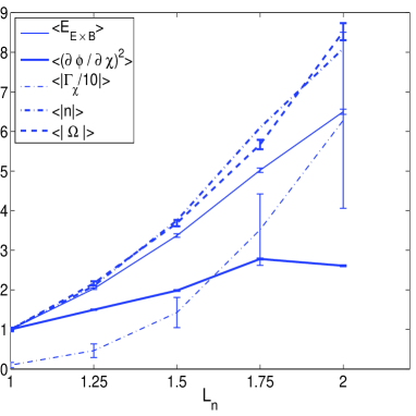
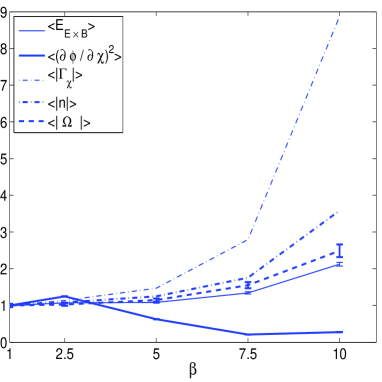
(a)  (b) 
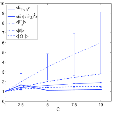
(c)  (d) 

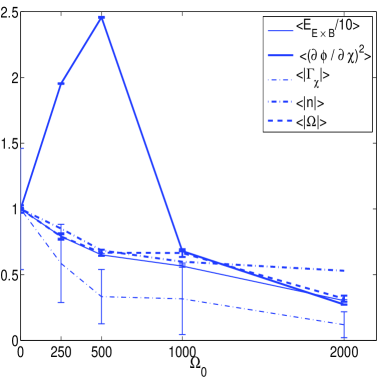
Figure 1: Global averages of the fluctuation kinetic energy $\langle E_{E\times B}\rangle=\langle\mathbf{v}_{E\times B}^{2}\rangle$ (thin solid line), zonal flow energy $\langle(\partial_{x}\phi)^{2}\rangle$ (bold solid line), radial transport $\langle\Gamma_{x}\rangle=\langle v_{E\times B,x}n\rangle$ (dash dotted line), density free energy $\langle|n|\rangle$ (bold dash dotted line), and average zonal flow shear $\langle\Omega\rangle=\langle\partial_{x}^{2}\phi\rangle$ (bold dashed line). Scalings with varying (a) density gradient length $L_{n}$, (b) collisionality $\hat{C}$, (c) normalised plasma beta $\hat{\beta}$, (d) imposed flow shear $\Omega_{0}=(\partial v_{ZF}/\partial x)_{0}$. Temporal standard deviations of the fluctuating global quantities are shown as error bars.

In figure (1 a) global averages (over the whole computational domain except boundary dissipation regions) of energetic quantities are shown. The global mean is in addition averaged over time during the saturated turbulent phase of the simulations, and the temporal standard deviations of the fluctuating global quantities are shown as error bars. The values are normalised with respect to the reference simulation $L_{n}=L_{n,0}$.

The zonal flow strength $v_{ZF}^{2}=\langle(\partial_{x}\Phi_{0})^{2}\rangle_{x}$, with $\Phi_{0}(x)=\langle\phi\rangle_{y,z}$, is doubled when the gradient is steepend corresponding to half the reference gradient length. The zonal flow shear $\Omega_{0}=\langle\partial_{x}^{2}\Phi_{0}\rangle$ increases by an order of magnitude, similar to the average free energy density $\langle|n|\rangle$. The radial density transport, defined as $\Gamma_{x}=nv_{E\times B,x}\sim n(\partial_{y}\phi)$, increases by nearly two orders of magnitude. The enhanced gradient drive is thus found to increase all turbulent activities.

In figure (2 a-1) the PDFs of the fluctuation auto-correlation $P(\tau_{AC})$ are shown for electrostatic potential perturbations $\phi$ on the negative axis, and density perturbations $n$ on the positive axis. Maxima of the auto-correlation time are found around $4~{}L_{\perp}/c_{s}$. For increasing density drive, secondary smaller peaks emerge around $1~{}L_{\perp}/c_{s}$. The mean value of density AC is lower by around $0.5~{}L_{\perp}/c_{s}$ compared to potential AC. Mean values of AC times are drawn as vertical lines.

Figure (2 a-2) shows on the negative and positive axes respectively the PDFs for two “typical” nonlinear time scales.

To estimate time scales for turbulent processes, we first introduce a “convective density time scale” $\tau_{conv}$ which should serve as a measure for the rate of change of the density, given by the continuity equation (which in the turbulent state is mainly determined by nonlinear convection): $\partial_{t}n\sim{\bf v}_{E\times B}\cdot\nabla n\equiv n/\tau_{conv}$ such that $\tau_{conv}\equiv(n/\partial_{t}n)=(n/|\mathbf{v}_{E\times B}\cdot\nabla n|)$.

As a second time scale, a measure of the local radial ExB velocity is introduced through ${\bf v}_{E\times B}\sim\partial_{y}\phi\equiv\rho_{s}/\tau_{E\times B}$, giving $\tau_{E\times B}\equiv\rho_{s}/\partial_{y}\phi$ in normalised units.

The PDF with respect to $\tau_{conv}$ is shown on the right half-space of fig. (2 a-2): no scaling of this time scale with gradient length is observable. The PDF with respect to $\tau_{E\times B}$ is shown on the left half-space of fig. (2 a-2): increasing the gradient drive (corresponding to smaller $L_{n}$) leads to a maximum of the PDF at smaller $\tau_{E\times B}$, which therefore can be interpreted as enhancing the radial $E\times B$ velocity. The correlation time of this maximum corresponds to the emerging second maximum in the auto correlation statistics of figure (2 a-1).

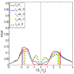
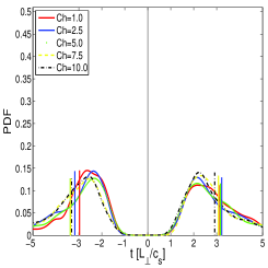
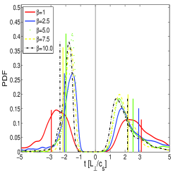
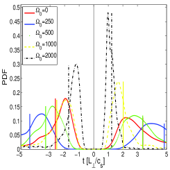
(a-1)  (a-2) 
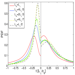
(b-1)  (b-2) 
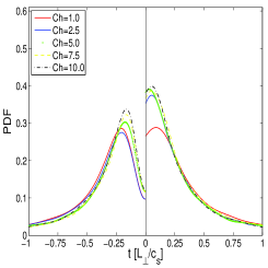
(c-1)  (c-2) 
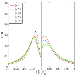
(d-1)  (d-2) 

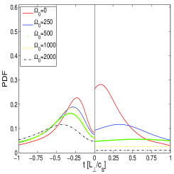
Figure 2: Temporal correlation scalings for (a) $L_{n}$, (b) $\hat{C}$, (c) $\hat{\beta}$, (d) $\Omega_{0}$: (1) auto-correlation PDFs for density (positive axis) and potential (negative axis); (2) PDFs of density convection time scale $\tau_{conv}$ (positive axis) and $E\times B$ time scale $\tau_{E\times B}$ (negative axis). Mean values of AC times are drawn as vertical lines.

For the correlation length analysis fluctuations of density $n$ and electrostatic potential $\phi$ have been recorded at three further positions, once radially separated by $\Delta x$ , once poloidally (or rather, perpendicular to radius and magnetic field in the drift plane) by $\Delta y$, and also along the magnetic field line by $\Delta z$. Correlation length PDFs $P(\lambda_{x})$, $P(\lambda_{y})$, $P(\lambda_{z})$, as defined in eq. (21), are shown in fig. (3 a) for increasing density gradient $L_{n}$.

The potential correlation lengths, drawn as PDFs on the negative axis of plots (3 a), show a slight rise in correlation lengths radially and poloidally, whereas the correlation length along the magnetic field line is slightly reduced when $L_{n}$ is increased. The density PDFs (on the positive axis) show an increase in events with short spatial correlations, both radially and in parallel, whereas for larger scales the probability is reduced. The density PDFs in poloidal direction remain nearly unchanged.

All spatial correlation length PDF appear to be far from Gaussian, with a steep peak at small scales and long tails for larger correlation lengths. The perpendicular scales are consistent with dominant turbulent vortex structures of the order of a few $\rho_{s}k_{\perp}$. The net effect from an increased density gradient in the constant in general are slightly smaller spatial correlation lengths for density fluctuations.

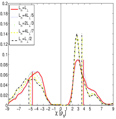
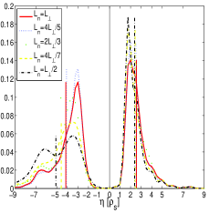
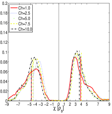
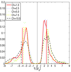
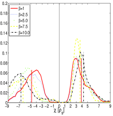
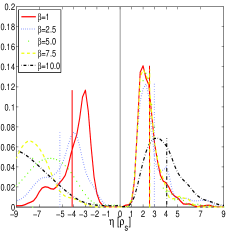
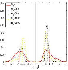
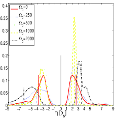
(a-1)  (a-2)  (a-3) 
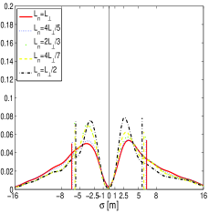
(b-1)  (b-2)  (b-3) 
(c-1)  (c-2)  (c-3) 
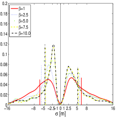
(d-1)  (d-2)  (d-3) 

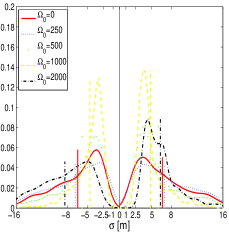
Figure 3: Correlation length PDFs scalings with (a) $L_{n}$, (b) $\hat{C}$, (c) $\hat{\beta}$, (d) $\Omega_{0}$: (1) radial, (2) poloidal (perpendicular), (3) parallel direction.

IV.2 Collisionality scaling

Next, the effect of reduced collisionality on edge turbulence correlations is analyzed. The collisionality $\hat{C}\propto 1/T_{e}$ scales inversely with the electron temperature $T_{e}$. In table (1) the parameters used for this simulation series are summarised. A collisionality parameter $\hat{C}=1$ corresponds to a roughly doubled temperature compared to $\hat{C}=10$.

In fig. (1 b) the energetics scaling with collisionality is shown. Except for the zonal flow energy $\langle v_{ZF}^{2}\rangle$ all global energy averages increase linearly with collisionality. For the radial density transport $\Gamma_{x}$ not only the mean value, but the fluctuation width (drawn as vertical deviation bars around the mean) increases.

In fig. (2 b) AC times of density and potential fluctuations are shown. Mean values of AC times, drawn as vertical lines in fig. (2 b-1), show no clear scaling with collisionality. Only the $E\times B$ AC time, on the negative half in fig. (2 b-2), shows a clear decrease for increasing $\hat{C}$.

All time scales are as usual normalized to the drift drift time scale $L_{\perp}/c_{s}$. In this series of simulations, however, $L_{\perp}/c_{s}$ is varied (according to table 1) in addition to $\hat{C}$. The reverse scaling of $\tau_{E\times B}$ with $T_{e}$, which is evident in fig. (2 b-2) in this $T_{e}$-dependent normalization, would also be qualitatively preserved if $\tau_{E\times B}$ were plotted in physical units (with the $T_{e}$ dependent normalization eliminated).

Spatial correlation lengths, shown in fig. (3 b), do not reveal any clear change in the correlation of fluctuation signals with collisionality.

Sim.	$\hat{C}$	$T_{e}$	$n_{0}$	$L_{\perp}/c_{s}$	$\rho_{s}$
no.		$[eV]$	$[10^{18}\;m^{-3}]$	$[10^{-6}\;s]$	$[10^{-3}\;m]$
1	1.0	51.8	$5.56$	$0.80$	1.00
2	2.5	38.2	$7.60$	$0.93$	8.93
3	5.0	30.3	$9.51$	$1.00$	7.95
4	7.5	26.5	$10.9$	$1.12$	7.43
5	10.0	24.0	$12.0$	$1.18$	7.10

Table 1: Parameters for simulations with increasing collisionality $\hat{C}$

IV.3 Plasma beta scaling

In the H-mode the plasma pressure in the pedestal is elevated. For constant magnetic field strength, the plasma beta $\beta=n^{2}T^{2}/\mu_{0}^{2}/B^{2}$ rises. This motivates the following simulation series, where the magnetic beta is increased, while keeping the collisionality constant. The variation of the electron temperature $T_{e}$, the particle density $n$, the time and space scales for the various simulation runs are listed in table (2).

The global energetics are shown in fig. (1 c). A reduction of zonal flows (drawn as solid line) to about a third for the $\hat{\beta}=10$ compared to the reference parameter case ($\hat{\beta}=1$), is caused by the enhanced Maxwell stress Naulin05 .

The zonal flow shear, the density free energy, the $E\times B$ flow energy as well as the radial $E\times B$ density transport increase with beta.

In fig. (2 c-1) the AC PDFs $P(\tau_{AC}(n))$, drawn in the positive half space, show a slight decrease of $\tau_{AC}=3~{}L_{\perp}/c_{s}$ down to $\tau_{AC}=2~{}L_{\perp}/c_{s}$ for beta rising from $1$ to $10$.

Comparison with the $E\times B$ and convective timescales on the negative and positive sides of fig. (2 c-2) shows that the lowered AC time for density fluctuations is accompanied by an an increasing turbulent $E\times B$ drift velocity. The convective time scale shifts to larger values for rising magnetic beta.

The perpendicular spatial correlation length PDFs for the potential, $P(\lambda_{x})$ and $P(\lambda_{y})$ in fig. (3 c-1,2), show growing tails (negative axis). The perpendicular size of potential structures grows with beta. Together with an increasing fluctuation energy this results in nearly unchanged mean decorrelation times $\tau_{AC}$, refered from the mean of $P(\tau_{AC})$, drawn on the negative half-space of figure (2 c-1).

The size of density perturbations increasingly differs from the potential perturbations due to the higher non-adiabaticity (via magnetic flutter) of the electrons. The result is an average density correlation length of $\lambda_{x}\sim\lambda_{y}\sim 4\rho_{s}$ for the density, and $\lambda_{x}\sim 7\rho_{s}$ and $\lambda_{y}\sim 6\rho_{s}$ for the potential at $\hat{\beta}=10.0$.

Along magnetic field lines $P(\lambda_{z})$ drawn in fig. (3 c-3) shows a clear decrease in correlation lengths of both density and potential, caused by the enhanced magnetic flutter.

Sim.	$\hat{\beta}$	$T_{e}$	$n_{0}$	$L_{\perp}/c_{s}$	$\rho_{s}$
no.		$[eV]$	$[10^{18}\;m^{-3}]$	$[10^{-6}\;s]$	$[10^{-3}\;m]$
1	1.0	52	5.56	0.80	1.00
2	2.5	70	10.2	0.69	1.21
3	5.0	88	16.2	0.61	1.36
4	7.5	101	21.3	0.57	1.45
5	10.0	111	25.8	0.55	1.52

Table 2: Parameters for simulations with increasing magnetic $\hat{\beta}$

IV.4 Imposed shear flow scaling

Further, a simulation series has been performed with the aim of analysing the impact of an imposed sheared $E\times B$ mean flow on correlations.

An external electrostatic zonal potential field $\phi_{0}(x)$ is applied through the nonlinear advection operators as $[\phi,f]\rightarrow[\phi+\phi_{0},f]$:

$$\phi_{0}(x) = (1/2)\Omega_{0}\left(x+L_{x}/2\right)^{2}$$ (22)

$$v_{0}(x) = \Omega_{0}\left(x+L_{x}/2\right)$$ (23)

$$\partial_{x}v_{0}(x) = \Omega_{0}$$ (24)

The application of $\phi_{0}$ results in a radially increasing $E\times B$ mean drift flow with velocity $v_{0}$ and constant flow shear $\Omega_{0}=(0,250,500,1000,2000)$.

In fig. (1 d) the turbulent transport and fluctuation amplitudes show a reduction for all levels of an imposed flow shear. The zonal flow amplitude increases strongly for moderate $\Omega_{0}=250-500$ due to enhanced zonal vorticity coupling $v_{0}^{2}\sim\langle\Omega\rangle\langle R_{e}\rangle$ of the Reynolds stress drive. For larger $\Omega_{0}$ the zonal flows appear strongly reduced, when the Reynolds stress $R_{e}=\partial_{x}\phi\;\partial_{y}\phi$ is lowered by the quenched fluctuation amplitudes.

The fluctuation AC time PDF for the shear flow experiment in fig. (2 d-1) shows for $\Omega_{0}=250-500$ a shift of the maximum to higher AC times (around $3-4~{}L_{\perp}/c_{s}$) for both density and potential fluctuations. For higher values of $\Omega_{0}$ the maximum of the PDF shifts to smaller $\tau_{AC}$, and peaks sharply for the density along the positive axis of plot (2 d-1). Vertical lines indicate mean values $\langle\tau_{AC}\rangle_{t}$, which reflect first the trend to longer self correlation times and then a drop to shorter living structures.

To properly reflect the lifetime of a turbulent structure, the AC statistics should be computed from a fluctuation time series taken in a co-moving frame, or with the mean flow velocity subtracted from the field. At a fixed probe position (which has been applied here for consistency with experimental measurements) the AC statistics not only maps the eddie turnover, but also the background advection of the structure. The drop in the AC PDF in fig. (2 d-2) is therefore partly debted to the faster decay of perturbations, but also to the higher convective $E\times B$ velocity of convection.

Characteristic $E\times B$ convection times $\tau_{E\times B}$ drawn as PDFs in the left half space of fig. (2 d-2) increase for growing $\Omega_{0}$. This suggests that convection is mainly caused by the fixed background $E\times B$ mean flow, whereas the convection caused by $E\times B$ drift fluctuations are suppressed by the mean flow. Along the positive axis the PDFs flatten for increasing $\Omega_{0}$.

Spatial correlation PDFs are shown in fig. (3 d). For $\Omega_{0}=250-500$, the perpendicular functions $P(\lambda_{x})$, and $P(\lambda_{y})$ do not change significantly. Further increasing $\Omega_{0}$ gives a shift of radial correlation lengths to smaller values, for density from around $4~{}\rho_{s}$ to $3~{}\rho_{s}$.

The poloidal correlation function $P(\lambda_{y})(n)$ on the right half space of fig. (3 d-2) increases to around $3.5~{}\rho_{s}$ for maximal imposed flow strength, and the potential correlation PDF along the negative axis show an increase to $6~{}\rho_{s}$. PDFs in fig. (3 d-1,2) of perpendicular correlation lengths show that the average length for $\Omega_{0}=0$ is larger radially than poloidally for the density. For the imposed shear flow of amplitude $\Omega_{0}=2000$ perturbations of density as well as of $\phi$ are strained out poloidally and radially quenched.

Fig. (3 d-3) shows a slight reduction of parallel correlation length PDFs $P(\lambda_{z})$ with initially rising flow shear amplitude for both potential and density . For the largest values of the imposed flow shear (drawn as black dash dotted line) the parallel correlation length of $\phi$ increases from $6~{}m$ to about $8~{}m$. The density PDFs $P(\lambda_{z})(n)$ shows only a damping of events with a very low parallel correlation length $\lambda_{z}<2.5~{}m$.

V Conclusions

Correlation lengths of density and electrostatic potential fluctuations for conditions relevant to an L-mode tokamak edge plasma near the L-H transition have been analysed by numerical simulation of drift-Alfvén turbulence. Five parameter scalings have been independently performed: density gradient length $L_{n}$, the collisionality $\hat{C}$, the plasma beta $\hat{\beta}$, and by imposing a flow shear $\Omega_{0}$.

A reduction of $L_{n}$ (corresponding to a pedestal profile steepening) results in slightly enhanced perpendicular correlations lengths for $\phi$, and reduced correlation lengths along the magnetic field lines.

Reducing collisionality $\hat{C}$ (corresponding to a rise in pedestal temperature) did not show any clear and significant scaling of all correlation lengths.

Increasing the plasma beta $\hat{\beta}$ has different effects on density and potential correlations. Perpendicular correlation lengths for $\phi$ increase, whereas the density correlation length PDF is shifted to smaller spatial scales. Parallel correlation lengths are reduced for both $n$ and $\phi$.

Externally imposing a flow shear $\Omega_{0}$ was found to significantly enhance poloidal and parallel correlations lengths of $\phi$ only for very strong shearing rates. Density correlation lengths are increased poloidally but are reduced along magnetic field lines. Radially a reduction of correlation amplitudes of $n$ and $\phi$ has been found.

It can be concluded from these parameter scaling simulations, that experimentally observed long-range correlations near or at the transition to H-mode states are likely caused by the straining effect of a strongly sheared flow on the turbulence. The zonal flows are amplified strongly only for moderate imposed mean flow shear, whereas long-range correlations appear only for strong external shearing. All other plasma parameters scalings, which appear towards a transition, have either a weak or reducing influence on correlation lengths.

References

- (1) R.A. Moyer, G.R. Tynan, C. Holland, M.J. Burin, Phys. Rev. Lett. 87, 135991 (2001).
- (2) M.A. Pedrosa, C. Silva, C. Hidalgo, B.A. Carreras, R.O. Orozco, D. Carralero, Phys. Rev. Lett. 100, 215003 (2008).
- (3) Y. Xu, S. Jachmich, R.R. Weynants, et al. Physics of Plasmas 16, 110704 (2009).
- (4) P. Manz, M. Ramisch, U. Stroth, Phys. Rev. E 82, 056403 (2010).
- (5) R.S. Wilcox, B.P. van Milligen, C. Hidalgo, et al. Nuclear Fusion 51, 083048 (2011).
- (6) Y. Xu, D. Carralero, C. Hidalgo, et al. Nuclear Fusion 51, 063020 (2011).
- (7) C. Silva, C. Hidalgo, M.A. Pedrosa, et al. Nuclear Fusion 51, 063025 (2011).
- (8) U. Stroth, P. Manz, M. Ramisch, Plasma Physics and Controlled Fusion 53, 024006 (2011).
- (9) B. Scott, Plasma Physics and Controlled Fusion 39, 1635 (1997).
- (10) D. Reiser, Physics of Plasmas 14, 08314 (2007).
- (11) P.F. Dunn, Measurement and data analysis for engineering and science. McGraw Hill, New York, 2005.
- (12) V. Naulin, A. Kendl, O.E. Garcia, A.H. Nielsen, J. Juul Rasmussen, Physics of Plasmas 12, 052515 (2005).