Transverse-Longitudinal Coupling by Space Charge in Cyclotrons

Abstract

A method is presented that enables to compute the parameters of matched beams with space charge in cyclotrons with emphasis on the effect of the transverse-longitudinal coupling. Equations describing the transverse-longitudinal coupling and corresponding tune-shifts in first order are derived for the model of an azimuthally symmetric cyclotron. The eigenellipsoid of the beam is calculated and the transfer matrix is transformed into block-diagonal form. The influence of the slope of the phase curve on the transverse-longitudinal coupling is accounted for. The results are generalized and numerical procedures for the case of an azimuthally varying field cyclotron are presented. The algorithm is applied to the PSI Injector II and Ring cyclotron and the results are compared to TRANSPORT.

Introduction

There is continuous interest in the understanding of space charge effects in isochronous cyclotrons Reiser ; Gordon5 ; Chasman ; Adam1 ; Adam2 ; Bertrand ; Pandit ; SIR1 ; Bi . The area is of special relevance for the conceptual designs of cyclotrons as energy-efficient drivers for accelerator driven systems (ADS) ADS0 ; ADS1 . Nevertheless there is no self-consistent first order theory of matched bunched beams with space charge in cyclotrons up to date known to the author. Bertrand and Ricaud showed that it is possible to set up and solve linearized equations of motion for a simple cyclotron model Bertrand , but they did not determine the parameters of matched beams in cyclotrons and they did not generalize their results in order to find a numerical method to compute matched beams for sector-focused cyclotrons. Information on the matched ellipsoid is of special interest for modern high-performance codes like OPAL, that enable to simulate high intensity beams in the space charge dominated regime HPC1 ; HPC2 .

First we describe the usual simplified azimuthally symmetric cyclotron model (see for instance Garren or Stammbach1 ), but include the linearized space charge forces. The model neglects possible effects of rf-acceleration and is restricted to the description of a coasting beam. A modified version of Teng’s method to decouple longitudinal and horizontal motion will be presented and applied to the simplified analytical model Teng ; EdwardsTeng . Later we describe how this method can be applied in an iterative numerical procedure to determine the parameters of matched beams with space charge in sector-focused cyclotrons. Finally we present some results as computed for the cyclotrons of the PSI high intensity accelerator facility.

I The simplified cyclotron model

The simplest relativistic cyclotron model is based on a magnetic field with cylindrical and mid-plane symmetrie. The nominal orbital frequency of an ion beam coasting in an isochronous cyclotron is

$$\omega_{o}={q\over m\,\gamma}\,B={q\over m\,\gamma}\,B_{0}\,\gamma\,,$$ (1)

where $q$ is the charge and $m$ the rest mass of the ions. The axial magnetic field is $B=B(r)=B_{0}\,\gamma$. We define a cyclotron length unit $a={c\over\omega_{o}}$ using the orbital frequency $\omega_{o}$. The particle velocity is $v=\omega_{o}\,r$ so that $\beta=v/c=r/a$. Hence the relativistic factor $\gamma$ can be written as

$$\gamma={1\over\sqrt{1-(r/a)^{2}}}\,.$$ (2)

The axial magnetic field in dependence of the radius $r$ is then given by

$$B(r)=B_{0}\,{1+\varepsilon(r)\over\sqrt{1-{r^{2}\over a^{2}}}}\,,$$ (3)

where $\varepsilon$ is a small distortion of the isochronism ($\varepsilon\ll 1$). The radial field increase compensates the relativistic mass increase and the cyclotron is strictly isochronous for $\varepsilon(r)=0$. The field index $n={r\over B}\,{dB\over dr}$ is given by

$$n={r\over B}\,{dB\over dr}\approx r\,{d\varepsilon\over dr}+\gamma^{2}-1\,,$$ (4)

so that

$$1+n\approx\gamma^{2}+r\,{d\varepsilon\over dr}\,.$$ (5)

The phase shift per turn $\Delta\phi\equiv{d\phi\over dn}$ is (see for instance Garren :

$$\begin{array}[]{rcl}\Delta\phi&=&T\,{d\phi\over dt}=T\,\left({d\phi_{hf}\over dt}-N_{h}\,{d\theta\over dt}\right)\\ &=&{2\,\pi\over\omega_{c}}\,\left(\omega_{hf}-N_{h}\,\omega_{c}\right)\\ &=&{2\,\pi\over\omega_{c}}\,\left(N_{h}\,\omega_{o}-N_{h}\,\omega_{c}\right)\\ &=&2\,\pi\,N_{h}\,\left({\omega_{o}\over\omega_{c}}-1\right)\,,\end{array}$$ (6)

where $\theta$ is the azimuthal angle, $\omega_{c}=\dot{\theta}$ is the real orbital frequency and $\omega_{hf}=N_{h}\,\omega_{o}$ the frequency of the accelerating high frequency system operated at the harmonic number $N_{h}$. The bending radius $r$ of a particle with charge $q$ in a magnetic field $B$ is given by $r={p\over q\,B}$ and hence $\omega_{c}$ can be written as

$$\begin{array}[]{rcl}\omega_{c}&=&{v\over r}={m\,c\,\gamma\,\beta\over m\,\gamma\,r}={p\over m\,\gamma\,r}\\ &=&{q\,B(r)\over m\,\gamma}={q\over m}\,{B_{0}\,\gamma\,(1+\varepsilon)\over\gamma}=\omega_{o}\,(1+\varepsilon)\\ \end{array}$$ (7)

so that

$$\begin{array}[]{rcl}{\omega_{o}\over\omega_{c}}&=&{1\over 1+\varepsilon}\approx 1-\varepsilon\\ \varepsilon&\approx&-{\Delta\phi\over 2\,\pi\,N_{h}}=-\left({\omega_{o}\over\omega_{c}}-1\right)\\ \end{array}$$ (8)

Hence ${d\varepsilon\over dr}$ is proportional to the change of the phase shift per turn with radius.

The reference orbit corresponding to the kinetic energy $E=m\,c^{2}\,(\gamma-1)=E_{0}\,(\gamma-1)$ is a circle with the radius

$$r(E)=a\,{\sqrt{\gamma^{2}-1}\over\gamma}\,.$$ (9)

We will use $x=r-r(E)$ as the horizontal coordinate of a specific orbit relative to the reference orbit, $y$ as the axial deviation from the median plane and $z$ as the longitudinal coordinate.

II Some General Remarks

From the assumption of midplane symmetrie it follows that the axial coordinate $y$ is not coupled neither to the horizontal nor to the longitudinal coordinate. Therefore it is sufficient to describe the coupling of horizontal and longitudinal motion. Since we assume azimuthal symmetrie, the matched beam ellipse must also be azimuthally symmetric, i.e. constant along the orbital length coordinate $s$. If the matched beam is constant, then the forces are constant - even if space charge is taken into account.

The vector describing the (horizontal and longitudinal) displacement of an orbit at position $s$ relative to the reference orbit is ${\bf x}=(x,x^{\prime},z,\delta)^{T}$ where $x^{\prime}={dx\over ds}$ is the horizontal direction angle with the reference orbit and $\delta={p-p_{0}\over p_{0}}$ is the momentum deviation. We use the formalism of linear Hamiltonian systems as for instance described by R. Talman Talman including the method of A. Wolski to compute the matched beam matrix Wolski . The equations of motion (to first order) can be written as

$${\bf x}^{\prime}(s)={\bf F}\,{\bf x(s)}\,,$$ (10)

where ${\bf F}$ is a constant $4\times 4$-matrix. The general solution is

$${\bf x}(s)=\exp{({\bf F}\,s)}\,{\bf x}(0)={\bf M}(s)\,{\bf x}(0)\,,$$ (11)

where ${\bf M}(s)$ is the transfer matrix. The matrix exponential ${\bf M}(s)$ is

$${\bf M}(s)=\exp{({\bf F}\,s)}={\bf 1}+{\bf F}\,s+{({\bf F}\,s)^{2}\over 2!}+{({\bf F}\,s)^{3}\over 3!}+\dots\,.$$ (12)

Let $S$ be the skew-symmetric matrix with $S^{2}=-1$

$$S=\left(\begin{array}[]{cccc}0&1&0&0\\ -1&0&0&0\\ 0&0&0&1\\ 0&0&-1&0\\ \end{array}\right)\,,$$ (13)

so that – since ${\bf M}$ is sympletic – the following relation holds:

$${\bf M}^{T}\,S\,{\bf M}=S\,.$$ (14)

If there exists an invertible transformation matrix $E$ and a diagonal matrix $\lambda$ such that

$${\bf F}={\bf E}\,\lambda\,{\bf E}^{-1}\,,$$ (15)

then its is easy to show that the following relation holds:

$${\bf M}={\bf E}\,\exp{(\lambda\,s)}\,{\bf E}^{-1}={\bf E}\,\Lambda\,{\bf E}^{-1}\,.$$ (16)

${\bf E}$ is the matrix of columnwise eigenvectors and $\lambda$ is the (diagonal) matrix of the corresponding eigenvalues of ${\bf F}$. The (imaginary) eigenvalues of ${\bf F}$ are the betatron frequencies of the orbital motion. ${\bf F}$ and ${\bf M}$ have the same eigenvectors – and the eigenvalues of ${\bf M}$ are the exponentials of the eigenvalues of ${\bf F}$. The eigenellipsoid $\sigma_{E}$ defined by

$$\sigma_{E}={\bf M}\,\sigma_{E}\,{\bf M}^{T}\,,$$ (17)

can then be written as follows Wolski :

$$\sigma_{E}=-{\bf E}\,{\cal D}\,{\bf E}^{-1}\,S\,,$$ (18)

where ${\cal D}$ is the diagonal matrix with the eigenvalues of $\sigma_{E}\,S$ – which are the emittances (apart from factors $\pm i$).

III The Equations of Motion (EQOM)

The Hamiltonian is given by

$$H={x^{\prime 2}\over 2}+{\delta^{2}\over 2\,\gamma^{2}}+{k_{x}-K_{x}\over 2}\,x^{2}-{\gamma^{2}\,K_{z}\over 2}\,l^{2}-h\,x\,\delta\,.$$ (19)

where the canonical coordinates are $x$ and $l$ and the momenta are given by $x^{\prime}$ and $\delta$. The EQOM (in first order) are:

$${d\over ds}\,\left(\begin{array}[]{c}x\\ x^{\prime}\\ l\\ \delta\\ \end{array}\right)=\left(\begin{array}[]{cccc}0&1&0&0\\ -k_{x}+K_{x}&0&0&h\\ -h&0&0&{1\over\gamma^{2}}\\ 0&0&K_{z}\,\gamma^{2}&0\\ \end{array}\right)\,\left(\begin{array}[]{c}x\\ x^{\prime}\\ l\\ \delta\\ \end{array}\right)\,,$$ (20)

where $h={1\over r}$ is the inverse bending radius and $k_{x}=h^{2}\,(1+n)$ is the horizontally restoring force. $K_{x}$ and $K_{z}$ represent the strength of the horizontal and longitudinal space charge forces Hinterberger :

$$\begin{array}[]{rclp{10mm}rcl}K_{x}&=&{K_{3}\,(1-f)\over(\sigma_{x}+\sigma_{y})\,\sigma_{x}\,\sigma_{z}}&&K_{3}&=&{3\,q\,I\,\lambda\over 20\,\sqrt{5}\,\pi\,\varepsilon_{0}\,m\,c^{3}\,\beta^{2}\,\gamma^{3}}\\ K_{z}&=&{K_{3}\,f\over\sigma_{x}\,\sigma_{y}\,\sigma_{z}}&&f&\approx&{\sqrt{\sigma_{x}\,\sigma_{y}}\over 3\,\gamma\,\sigma_{z}}\\ K_{y}&=&{K_{3}\,(1-f)\over(\sigma_{x}+\sigma_{y})\,\sigma_{y}\,\sigma_{z}}&&&&\\ \end{array}$$ (21)

The eigenvalues of ${\bf F}$ and ${\bf M}$ are:

$$\begin{array}[]{rcl}\lambda&=&\text{Diag}(i\,\Omega,-i\,\Omega,i\,\omega,-i\,\omega)\\ \Lambda&=&\text{Diag}(e^{i\,\Omega\,s},e^{-i\,\Omega\,s},e^{i\,\omega\,s},e^{-i\,\omega\,s})\\ a&\equiv&{k_{x}-K_{x}-K_{z}\over 2}\\ b&\equiv&K_{z}\,(K_{x}+h^{2}\,\gamma^{2}-k_{x})\\ \Omega&=&\sqrt{a+\sqrt{a^{2}-b}}\\ \omega&=&\sqrt{a-\sqrt{a^{2}-b}}\,.\end{array}$$ (22)

Note that $b$ must be positive to give a real–valued frequency $\omega$ and hence a longitudinally focused orbit. This is especially important, if we allow for a (small) field error $\varepsilon(r)$. In this case the change of the orbital frequency as given by ${d\varepsilon\over dr}$ can play a significant role:

$$\begin{array}[]{rcl}k_{x}&=&h^{2}\,(1+n)=h^{2}\,(1+r\,{d\varepsilon\over dr}+\gamma^{2}-1)\\ &=&h^{2}\,\left(\gamma^{2}+r\,{d\varepsilon\over dr}\right)=h^{2}\,\gamma^{2}+h\,{d\varepsilon\over dr}\\ b&=&K_{z}\,(K_{x}-h\,{d\varepsilon\over dr})\\ \end{array}$$ (23)

If $K_{x}<h\,{d\varepsilon\over dr}$, then the longitudinal focusing frequency $\omega$ is imaginary and the longitudinal beam size increases exponentially with $s$. This in fact is a surprising feature of this type of coupling in combination with isochronism: Longitudinal focusing requires a strong enough horizontally defocusing space charge force. On the other hand, if ${d\varepsilon\over dr}<0$, i.e. if the radial increase of the magnetic field is below the isochronous field increase, then the longitudinal focusing is strengthened.

The matrix of eigenvectors ${\bf E}$ of the force matrix ${\bf F}$ is

$${\bf E}=\left(\begin{array}[]{cccc}1&1&1&1\\ i\,\Omega&-i\,\Omega&i\,\omega&-i\,\omega\\ i\,\Omega\,A&-i\,\Omega\,A&i\,\omega\,B&-i\,\omega\,B\\ K_{z}\,\gamma^{2}\,A&K_{z}\,\gamma^{2}\,A&K_{z}\,\gamma^{2}\,B&K_{z}\,\gamma^{2}\,B\\ \end{array}\right)\,.$$ (24)

The inverse matrix ${\bf E}^{-1}$ is given by:

$${\bf E}^{-1}={1\over 2\,(A-B)}\left(\begin{array}[]{cccc}-B&{i\,B\over\Omega}&-{i\over\Omega}&{1\over K_{z}\,\gamma^{2}}\\ -B&{-i\,B\over\Omega}&{i\over\Omega}&{1\over K_{z}\,\gamma^{2}}\\ A&-{i\,A\over\omega}&{i\over\omega}&-{1\over K_{z}\,\gamma^{2}}\\ A&{i\,A\over\omega}&-{i\over\omega}&-{1\over K_{z}\,\gamma^{2}}\\ \end{array}\right)\,,$$ (25)

where

$$\begin{array}[]{rcl}A&=&{h\over\Omega^{2}+K_{z}}\\ B&=&{h\over\omega^{2}+K_{z}}\\ \end{array}$$ (26)

The transfer matrix ${\bf M}$ can be computed by using eq. 16 and one obtains:

$${\bf M}={1\over A-B}\,\left(\begin{array}[]{cccc}A\,c-B\,C&{A\,\tilde{s}\over\omega}-{B\,S\over\Omega}&{S\over\Omega}-{\tilde{s}\over\omega}&A\,B\,(C-c)\\ \Omega\,B\,S-\omega\,A\,\tilde{s}&A\,c-B\,C&C-c&A\,B\,(\omega\,\tilde{s}-\Omega\,S)\\ A\,B\,(\Omega\,S-\omega\,\tilde{s})&A\,B\,(c-C)&A\,C-B\,c&A\,B\,(B\,\omega\,\tilde{s}-A\,\Omega\,S)\\ c-C&{\tilde{s}\over\omega}-{S\over\Omega}&{S\over B\,\Omega}-{\tilde{s}\over A\,\omega}&A\,C-B\,c\\ \end{array}\right)\,,$$ (27)

where

$$\begin{array}[]{rclp{10mm}rcl}C&=&\cos{(\Omega\,s)}&&S&=&\sin{(\Omega\,s)}\\ c&=&\cos{(\omega\,s)}&&\tilde{s}&=&\sin{(\omega\,s)}\\ \end{array}$$ (28)

IV The Eigenellipsoid

The matrix ${\cal D}$ is explicitely given by ${\cal D}=\text{Diag}(i\,\varepsilon_{1},-i\,\varepsilon_{1},-i\,\varepsilon_{2},i\,\varepsilon_{2})$ Wolski . The matched eigenellipsoid can then be calculated using eq. 18:

$$\sigma_{E}={1\over B-A}\,\left(\begin{array}[]{cccc}{B\,\varepsilon_{1}\over\Omega}+{A\,\varepsilon_{2}\over\omega}&0&0&{\varepsilon_{1}\over\Omega}+{\varepsilon_{2}\over\omega}\\ 0&B\,\varepsilon_{1}\,\Omega+A\,\varepsilon_{2}\,\omega&{\varepsilon_{1}\,\Omega+\varepsilon_{2}\,\omega\over K_{z}\,\gamma^{2}}&0\\ 0&{\varepsilon_{1}\,\Omega+\varepsilon_{2}\,\omega\over K_{z}\,\gamma^{2}}&{A\,\varepsilon_{1}\,\Omega+B\,\varepsilon_{2}\,\omega\over K_{z}\,\gamma^{2}}&0\\ {\varepsilon_{1}\over\Omega}+{\varepsilon_{2}\over\omega}&0&0&{\varepsilon_{1}\over B\,\Omega}+{\varepsilon_{2}\over A\,\omega}\\ \end{array}\right)$$ (29)

The beam dimensions are given by the diagonal elements of the matrix representing the eigenellipsoid:

$$\begin{array}[]{rcl}\sigma_{x}^{2}&=&{1\over B-A}\left({B\,\varepsilon_{x}\over\Omega}+{A\,\varepsilon_{z}\over\omega}\right)\\ \sigma_{z}^{2}&=&{1\over B-A}\left({A\,\varepsilon_{x}\,\Omega+B\,\varepsilon_{z}\,\omega\over K_{z}\,\gamma^{2}}\right)\,,\end{array}$$ (30)

where $\varepsilon_{1}=\varepsilon_{x}$ and $\varepsilon_{2}=\varepsilon_{z}$ are identified with the horizontal and longitudinal emittance, respectively. The axial motion can be treated separately and one finds

$$\sigma_{y}^{2}={\varepsilon_{y}\over\sqrt{h^{2}\,\nu_{y}^{2}-K_{y}}}\,.$$ (31)

If one considers EQ. LABEL:eq_Kxyz together with EQ. 30 and EQ. 31, then it is obvious, that this result does not enable to start a straightforward calculation, since the beam sizes depend on the space charge forces and vice versa in an algebraically complicated way. But with the additional assumption of a spherical beam, it is possible to derive a 4th order equation for the beam size as will be shown in Sec. VII.

V Decoupling Longitudinal and Transverse Motion

If sectors are considered, then the azimuthal symmetrie is broken and hence the force terms in the EQOM and consequently the beam ellipsoid depend on the position $s$. The vertical beam dynamics can still be treated separately, but is has to be taken into account that the periodic change of the vertical beam size influences the space charge factors $K_{x}$ and $K_{z}$. The design orbit usually has to be computed numerically as described by Gordon Gordon . If this has been done, it is possible to compute the transfer matrix for known starting conditions, since the equations of motion are known and can be integrated. The problem is to find the correct beam dimensions for a given beam current and given emittances such that the beam is matched, i.e. such that EQ. 17 is fulfilled.

Teng and Edwards described a parametrization for coupled motion in two and more dimensions that allows to find the decoupling matrix Teng ; EdwardsTeng . They called their method symplectic rotation. We will give a brief summary of the method and apply it to the problem of decoupling longitudinal and transverse motion.

Given two $2\times 2$ symplectic matrices ${\cal A}$ and ${\cal B}$ that form a block-diagonal (i.e. decoupled) transfer matrix $T_{0}$:

$$\begin{array}[]{rcl}T_{0}&=&\left(\begin{array}[]{cc}{\cal A}&0\\ 0&{\cal B}\end{array}\right)\\ {\cal A}(\mu_{1})&=&\cos{(\mu_{1})}\,{\bf 1}+\sin{(\mu_{1})}\,\left(\begin{array}[]{cc}\alpha_{1}&\beta_{1}\\ -\gamma_{1}&-\alpha_{1}\end{array}\right)\\ {\cal B}(\mu_{2})&=&\cos{(\mu_{2})}\,{\bf 1}+\sin{(\mu_{2})}\,\left(\begin{array}[]{cc}\alpha_{2}&\beta_{2}\\ -\gamma_{2}&-\alpha_{2}\end{array}\right)\,,\end{array}$$ (32)

where $\alpha_{i}$, $\beta_{i}$ and $\gamma_{i}$ are the familiar twiss-parameters. Then a general symplectic transfer matrix ${\bf M}$ of coupled motion can be written as

$${\bf M}=\left(\begin{array}[]{cc}M&n\\ m&N\end{array}\right)={\bf R}\,T_{0}\,{\bf R}^{-1}\,.$$ (33)

where $M$, $N$, $m$ and $n$ are $2\times 2$ matrices and ${\bf R}$ is the symplectic rotation matrix. Teng suggested to write ${\bf R}$ in the form

$$\begin{array}[]{rcl}{\bf R}&=&\left(\begin{array}[]{cc}I\,\cos{(\phi)}&D^{-1}\,\sin{(\phi)}\\ -D\,\sin{(\phi)}&I\,\cos{(\phi)}\end{array}\right)\\ {\bf R}^{-1}&=&\left(\begin{array}[]{cc}I\,\cos{(\phi)}&-D^{-1}\,\sin{(\phi)}\\ D\,\sin{(\phi)}&I\,\cos{(\phi)}\end{array}\right)\,.\end{array}$$ (34)

where $D$ is a symplectic $2\times 2$ transfer matrix that describes the structure of the coupling. Then one obtains Teng ; EdwardsTeng :

$$\begin{array}[]{rcl}M&=&{\cal A}\,\cos^{2}{(\phi)}+D^{-1}\,{\cal B}\,D\,\sin^{2}{(\phi)}\\ N&=&{\cal B}\,\cos^{2}{(\phi)}+D\,{\cal A}\,D^{-1}\,\sin^{2}{(\phi)}\\ m&=&-(D\,{\cal A}-{\cal B}\,D)\,\sin{(\phi)}\,\cos{(\phi)}\\ n&=&-({\cal A}\,D^{-1}-D^{-1}\,{\cal B})\,\sin{(\phi)}\,\cos{(\phi)}\\ \end{array}$$ (35)

The rotation angle $\phi$ can be computed using

$$\begin{array}[]{rcl}\frac{1}{2}\,Tr(M-N)&=&\cos{(2\,\phi)}\,(\cos{(\mu_{1})}-\cos{(\mu_{2})})\\ 2\,Det(m)+Tr(n\,m)&=&\sin^{2}{(2\,\phi)}\,(\cos{(\mu_{1})}-\cos{(\mu_{2})})^{2}\,,\end{array}$$ (36)

If we apply this method to the transfer matrix computed according to EQ. 16, we obtain:

$$\begin{array}[]{rcl}\frac{1}{2}\,Tr(M-N)&=&{B+A\over B-A}\,(\cos{(\Omega s)}-\cos{(\omega s)})\\ 2\,Det(m)+Tr(n\,m)&=&-{4\,A\,B\over(B-A)^{2}}\,(\cos{(\Omega s)}-\cos{(\omega s)})^{2}\,,\end{array}$$ (37)

Comparison yields:

$$\begin{array}[]{rcl}\cos{(2\,\phi)}&=&{B+A\over B-A}\\ \sin^{2}{(2\,\phi)}&=&-{4\,A\,B\over(B-A)^{2}}\\ \end{array}$$ (38)

From EQ. LABEL:eq_AB_def we find that $A>0$ and $B>0$ and $B>A$ since $\Omega^{2}>\omega^{2}$, so that the method fails in the case under study. The method of symplectic rotation is not generally applicable and has to be extended. A workaround solution was found by replacing trigonometic by hyperbolic functions.

$$\begin{array}[]{rcl}{\bf R}&=&\left(\begin{array}[]{cc}I\,\cosh{(\psi)}&D^{-1}\,\sinh{(\psi)}\\ D\,\sinh{(\psi)}&I\,\cosh{(\psi)}\end{array}\right)\\ {\bf R}^{-1}&=&\left(\begin{array}[]{cc}I\,\cosh{(\psi)}&-D^{-1}\,\sinh{(\psi)}\\ -D\,\sinh{(\psi)}&I\,\cosh{(\psi)}\end{array}\right)\,,\end{array}$$ (39)

with $Det(D)=-1$, i.e. $D$ is not symplectic – but ${\bf R}$ is symplectic.

	Symplectic Rotation	“Symplectic Boost”
$Tr(M-N)/2$	$\cos{(2\,\phi)}\,\Delta$	$\cosh{(2\,\psi)}\,\Delta$
$D_{t}$	$\sin{(2\,\phi)}^{2}\,\Delta^{2}$	$-\sinh{(2\,\psi)}^{2}\,\Delta^{2}$
$D$	$-{m+S_{2}\,n^{T}\,S_{2}^{T}\over\Delta\,\sin{(2\,\phi)}}$	${m+S_{2}\,n^{T}\,S_{2}^{T}\over\Delta\,\sinh{(2\,\psi)}}$
${\cal A}$	$M-D^{-1}\,m\,\tan{(\phi)}$	$M-D^{-1}\,m\,\tanh{(\psi)}$
${\cal B}$	$N+D\,n\,\tan{(\phi)}$	$N-D\,n\,\tanh{(\psi)}$

Table 1: Comparison of the method of symplectic rotation with the symplectic “Lorentz boost”. The difference $\Delta$ is defined by $\Delta\equiv\cos{(\mu_{1})}-\cos{(\mu_{2})}$. The matrix $S_{2}$ is defined by $S_{2}=\left(\begin{array}[]{cc}0&1\\ -1&0\end{array}\right)$ and $D_{t}$ is defined by $D_{t}=2\,Det(m)+Tr(n\,m)$.

Tab. 1 compares the formulas of the symplectic rotation and of symplectic “Lorentz boost”. Applying this method to the case under study then gives:

$$\begin{array}[]{lclp{5mm}lcl}\sinh{(2\,\psi)}&=&{2\,\sqrt{A\,B}\over B-A}&&\cosh{(2\,\psi)}&=&{B+A\over B-A}\\ \tanh{(2\,\psi)}&=&{2\,\sqrt{A\,B}\over B+A}&&\sinh{(\psi)}&=&\sqrt{A\over B-A}\\ \cosh{(\psi)}&=&\sqrt{B\over B-A}&&\tanh{(\psi)}&=&\sqrt{A\over B}\,,\end{array}$$ (40)

which can be solved. The matrices ${\cal A}$ and ${\cal B}$ are then given by:

$$\begin{array}[]{rcl}{\cal A}&=&\left(\begin{array}[]{cc}\cos{(\Omega s)}&\sin{(\Omega s)}/\Omega\\ -\Omega\,\sin{(\Omega s)}&\cos{(\Omega s)}\end{array}\right)\\ {\cal B}&=&\left(\begin{array}[]{cc}\cos{(\omega s)}&-A\,B\,\omega\,\sin{(\omega s)}\\ \sin{(\omega s)}/(A\,B\,\omega)&\cos{(\omega s)}\end{array}\right)\\ D&=&\left(\begin{array}[]{cc}0&\sqrt{A\,B}\\ 1/\sqrt{A\,B}&0\end{array}\right)\\ \end{array}$$ (41)

The signs in ${\cal B}$ suggest a negative $\beta_{2}$ - but this can be compensated by using either a negative emittance or a negative frequency $\omega$, since the transfer matrix is invariant against a change of the sign of $\omega$, while $\sigma_{E}$ is not.

The transformation matrices are explicitely given by:

$$\begin{array}[]{rcl}{\bf R}&=&{\sqrt{B\over B-A}}\,\left(\begin{array}[]{cccc}1&0&0&A\\ 0&1&1/B&0\\ 0&A&1&0\\ 1/B&0&0&1\\ \end{array}\right)\\ &&\\ {\bf R}^{-1}&=&{\sqrt{B\over B-A}}\,\left(\begin{array}[]{cccc}1&0&0&-A\\ 0&1&-1/B&0\\ 0&-A&1&0\\ -1/B&0&0&1\\ \end{array}\right)\,.\end{array}$$ (42)

Note: ${\bf R}$ and ${\bf R}^{-1}$ are symplectic. To make the method complete, we give the formula to split $2\times 2$ matrices of the form of ${\cal A}$ or ${\cal B}$:

$$\begin{array}[]{rcl}c&=&\cos{\mu}\\ s&=&\sin{\mu}\\ \left(\begin{array}[]{cc}c&s/K\\ -K\,s&c\\ \end{array}\right)&=&R_{2}\,\left(\begin{array}[]{cc}e^{-i\,\mu}&0\\ 0&e^{i\,\mu}\\ \end{array}\right)\,R_{2}^{-1}\\ R_{2}&=&\left(\begin{array}[]{cc}i/K&-i/K\\ 1&1\\ \end{array}\right)\\ R_{2}^{-1}&=&\left(\begin{array}[]{cc}-i\,K/2&1/2\\ i\,K/2&1/2\\ \end{array}\right)\\ \end{array}$$ (43)

The matched beam ellipsoid can be computed for given emittances according to EQ. 18 as soon as the diagonalization of the transfer matrix ${\bf M}$ is known.

The fact that we have to extend the decoupling method of Teng and Edwards raises the question, whether the description of decoupling is now complete or if there are other cases that require further modifications or extensions. The answer to this question requires a proper two-dimensional extension of the Courant-Snyder theory and a complete survey of all possible symplectic transformations as presented in an accompanying paper rdm_paper .

VI The Iteration Process and Examples

We have shown for the symmetric analytical example that a modified version of the method of Teng and Edwards enables to bring the transfer matrix in block-diagonal form according to EQ. 32. The diagonalization of the block-diagonal matrices is given by EQ. LABEL:eq_diag2 and hence the matrix of eigenvectors $E$ and the matched beam ellipsoid can be constructed.

In order to take advantage of this method for the case of sectored cyclotrons, the method has to be applied iteratively. The goal is to compute the properties of a matched beam. Assumed that the beam emittances and the current are given as boundary conditions, one proceeds as follows:

1. Provide an initial guess of the beam dimensions $\sigma_{x}(s)$, $\sigma_{y}(s)$ and $\sigma_{z}(s)$.

2. Compute the driving terms of the space charge forces $K_{x}(s)$, $K_{y}(s)$ and $K_{z}(s)$.

3. Compute the one-turn transfer matrix ${\bf M}(s)$ for all azimuthal angles.

4. Compute the eigenvectors of ${\bf M}(s)$ by diagonalization.

5. Use the beam emittances to obtain the eigenellipsoid $\sigma_{E}$ according to EQ. 18.

6. Take the beam sizes from $\sigma_{E}$ and go back to step 2, if beam sizes changed significantly compared to the previous iteration.

Optionally one can start the iteration with a reduced beam current and increase it either during the iteration process or use the result of the reduced beam current as an initial guess for higher currents. The (speed of) convergence strongly depends on the assumptions about beam current and emittance. In the following examples, the process converged typically after less than 20 iterations.

VI.1 Example: PSI Injector II

The PSI high intensity proton accelerator facility MikePierre ; Mike2008 (HIPA) consists of a Cockcroft-Walton pre-accelerator, a four-sector injector cyclotron (Injector II, $72\,\mathrm{MeV}$) and the eight sector Ring cyclotron ($590\,\mathrm{MeV}$). In routine operation the beam current is $2.2\,\mathrm{mA}$.

The Injector II cyclotron can be modelled reasonably well by a hard edge approximation of the sector magnets. This has the advantage that the computed matched beam parameters can be compared to TRANSPORT transport1 ; transport2 ; transport3 . We have computed the matched beam parameters for Injector II. The results have then be used as input parameters for TRANSPORT (with space charge). The results are shown in Fig. 1.

Figure 1: Transport (re-)computation of a matched beam in Injector II for a circulating beam of $2.2\,\mathrm{mA}$ at low energy. The boxes indicate the position of the sector magnets SM1..SM4. The horizontal beam width is plotted as a negative value. The longitudinal beam size is plotted as $2\,\sigma_{z}$.

VI.2 Example: PSI Ring Cyclotron

The PSI ring cyclotron is a separated sector isochronous cyclotron with 8 sectors. But since the field of the magnets does not fall off as sharp as it does in Injector II, a hard edge approximation does not work equally well. Furthermore the sectors are much more spiralled. For the sake of precision we used the measured field map $B(r,\theta)$ to compute the equilibrium orbits (EO) on a radial grid eo_paper .

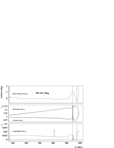
Figure 2: Top: Phase shift per turn for the ring cyclotron computed from the measured magnetic field map. Middle: Horizontal and vertical betatron-tunes of the Ring-cyclotron as computed by EO-code (gray solid lines), the transfer matrix method over the EO (black solid lines) and with space charge (dashed lines). Bottom: Longitudinal betatron tune as induced by transverse–longitudinal coupling. The region with a negative slope of the phase shift is indicated by vertical lines. Without further field trimming, the longitudinal focusing is suppressed by the term $-h\,{d\varepsilon\over dr}$ and the longitudinal beam size may increase. The calculation has been performed for a beam current of $2.2\,\mathrm{mA}$ and $(\varepsilon_{x},\varepsilon_{y},\varepsilon_{z})=(1.5,2.5,0.5)\,\mathrm{\pi mmmrad}$.

The radius $R_{eo}(\theta)$ of the equilibrium orbit (EO) is then given as a function of the angle and of the starting radius $R_{eo}(\theta_{0})$. Besides the pure geometry of the orbit one also obtains a precise value for $\varepsilon=1-{\omega_{o}\over\omega}$ for each EO Gordon , which then allows to compute ${d\varepsilon\over dr}$. In order to obtain the force matrix according to EQ. 20, the following additional calculations have been done:

1. Inverse bending radius $h={1\over\rho}={B(r,\theta)\over B_{0}\,p}$

2. Local field index

   $$n={\rho\over B}\,{dB\over dx}={B_{0}\over B^{2}}\,\left({dB\over dr}\,p_{\theta}-{dB\over r\,d\theta}\,p_{r}\right)\,.$$

3. Path length element $\Delta s=\sqrt{r^{\prime 2}+r^{2}}\,\Delta\theta$.

4. Horizontal (vertical) focusing $k_{x}={1+n\over\rho^{2}}$ ($k_{y}={-n\over\rho^{2}}$).

5. $h(E,\theta)$, $n(E,\theta)$, $\gamma(E)$ and the space charge forces $K_{x}$ , $K_{y}$ , $K_{z}$ are then used to compose the force matrix ${\bf F}$.

6. The exponential series allows to compute the transfer matrix for a (short) interval $[\theta\dots\theta+\Delta\theta]$:

   $${\bf M}=\exp{(F\,\Delta s)}=1+F\,\Delta s+{F^{2}\over 2!}\,\Delta s^{2}+\dots$$ (44)

   (Typically $3\dots 4$ terms are sufficient.)

7. Multiplication of all matrices yields the one-turn transfer matrix ${\bf M}$.

8. Diagonalize ${\bf M}$ and compute eigenellipse $\sigma_{E}$.

9. The average beam sizes are obtained from the eigenellipsoid and used to recompute the force coefficients.

10. The convergence is then checked and either the next iteration starts with step 5) or is stopped.

Fig. 2 shows some results of the matched beam with space charge for the PSI ring cyclotron, the phase shift per turn vs. energy in the upper, the transversal tunes in the second and the axial tune in the last graph. The region where the slope of the phase shift is negative has been marked by vertical lines. In this region the longitudinal tune due to space charge forces apparently becomes imaginary.

VII Spherical Symmetry

The first item in the described algorithm is to provide an initial guess of the beam dimensions. In the following we show how to obtain a possible choice of the initial guess for “nearly” spherical beams. If the horizontal-longitudinal coupling is strong enough, the beam will usually be approximately circular in this plane Stammbach2 . The axial size depends mainly on the vertical emittance and tune.

From EQ. 22 and EQ. LABEL:eq_AB_def one quickly derives:

$$\begin{array}[]{rcl}\Omega^{2}\,\omega^{2}&=&K_{z}\,(K_{x}+h^{2}\,\gamma^{2}-k_{x})\\ \Omega^{2}+\omega^{2}&=&k_{x}-K_{x}-K_{z}\\ \Omega^{2}-\omega^{2}&=&\sqrt{(k_{x}-K_{x}+K_{z})^{2}-4\,h^{2}\,\gamma^{2}\,K_{z}}\\ {1\over B-A}&=&{\gamma^{2}\,h\,K_{z}\over\sqrt{(k_{x}-K_{x}+K_{z})^{2}-4\,h^{2}\,\gamma^{2}\,K_{z}}}\\ \end{array}$$ (45)

With the assumption of an isochronous cyclotron ($k_{x}=h^{2}\,\gamma^{2}$) and spherical symmetrie, i.e.

$$\begin{array}[]{rcl}\sigma&=&\sigma_{x}=\sigma_{y}=\sigma_{z}\,\gamma\\ \varepsilon&=&\varepsilon_{x}=\varepsilon_{y}=\varepsilon_{z}\\ \rightarrow&&K=K_{x}=K_{y}=K_{z}={K_{3}\,\gamma\over 3\,\sigma^{3}}\\ \end{array}$$ (46)

one finds

$$\begin{array}[]{rcl}\Omega^{2}\,\omega^{2}&=&K^{2}\\ \Omega^{2}+\omega^{2}&=&k_{x}-2\,K\\ \Omega^{2}-\omega^{2}&=&\sqrt{k_{x}^{2}-4\,K\,k_{x}}\\ {1\over B-A}&=&{K\over h\,\sqrt{1-4\,K/k_{x}}}\\ \end{array}$$ (47)

The beam size $\sigma$ then yields using EQ. 30:

$$\begin{array}[]{rcl}\sigma^{4}&=&\varepsilon^{2}\,{(B\,\omega+A\,\Omega)^{2}\over(\Omega\,\omega)^{2}\,(B-A)^{2}}\\ &=&{4\,\varepsilon^{2}\over k_{x}-4\,K}\,,\end{array}$$ (48)

so that one obtains

$$\sigma^{4}-{4\,K_{3}\,r^{2}\over 3\,\gamma}\,\sigma-{4\,\varepsilon^{2}\,r^{2}\over\gamma^{2}}=0\,.$$ (49)

If one defines $\sigma_{0}=\sqrt{2\,r\,\varepsilon\over\gamma}$, then EQ. 49 can be written as

$$x^{4}-\alpha\,x-1=0\,,$$ (50)

where

$$\begin{array}[]{rcl}x&=&{\sigma\over\sigma_{0}}\\ \alpha&=&{4\,K_{3}\,r^{2}\over 3\,\gamma\,\sigma_{0}^{3}}={K_{3}\,\sqrt{2\,\gamma\,r}\over 3\,\varepsilon^{3/2}}>0\,.\end{array}$$ (51)

A polynom of 4th order has 4 solutions, namely the solutions of EQ. 50 are

$$x={1\over 2\,6^{1/3}}\,\left(\sqrt{Y}\pm\,\sqrt{\pm\,{12\,\alpha\over\sqrt{Y}}-Y}\right)\,,$$ (52)

where the abbreviations used are defined by

$$\begin{array}[]{rcl}Y&=&2^{1/3}\,Z-{8\,3^{1/3}\over Z}\geq 0\\ Z&=&(9\,\alpha^{2}+\sqrt{3}\,\sqrt{256+27\,\alpha^{2}})^{1/3}>768^{1/6}\,.\end{array}$$ (53)

The minus sign in the square root of EQ. 52 belongs to a pair of complex conjugate solutions and may not be used. Starting from low values of $\alpha$, $Y$ monotonically increases starting from zero so that we have to take the plus in front of the square root as well in order to obtain positive solutions also for small values of $\alpha$, so that

$$x={1\over 2\,6^{1/3}}\,\left(\sqrt{Y}+\sqrt{{12\,\alpha\over\sqrt{Y}}-Y}\right)\,.$$ (54)

Analyzing EQ. 50 one finds that

$$\begin{array}[]{rcl}\lim\limits_{\alpha\to 0}\,x(\alpha)&=&1\\ \lim\limits_{\alpha\to\infty}\,x(\alpha)&=&\alpha^{1/3}\,,\end{array}$$ (55)

so that the function $x(\alpha)=(1+\alpha)^{1/3}$ is a reasonable approximation. The maximal relative deviation of about $-0.035$ appears at $\alpha\approx 3/2$. Therefore we suggest to use the approximations

$$\sigma\approx\left\{\begin{array}[]{lcl}\sigma_{0}\,(1+{\alpha\over 4}-{\alpha^{2}\over 32})&\mathrm{for}&0\leq\alpha\leq 5/2\\ \sigma_{0}\,(1+\alpha)^{1/3}&\mathrm{for}&5/2\leq\alpha\\ \end{array}\right.\,.$$ (56)

Using the normalized emittance $\bar{\varepsilon}=\beta\,\gamma\,\varepsilon$, the wavelength $\lambda={c\over\nu_{rf}}={2\,\pi\,c\over\omega_{o}\,N_{h}}$, the cyclotron radius $a={c\over\omega_{0}}={r\over\beta}$ and the relation $\varepsilon_{0}\,c^{2}={1\over\mu_{0}}$, the values of $K_{3}$, $\alpha$ and $\sigma_{0}$ can be written as follows:

$$\begin{array}[]{rcl}K_{3}&=&{3\,q\,I\,\lambda\over 20\,\sqrt{5}\,\pi\,\varepsilon_{0}\,m\,c^{3}\,\beta^{2}\,\gamma^{3}}\\ &=&{3\,q\,\mu_{0}\,I\,a\over 10\,\sqrt{5}\,m\,c\,\beta^{2}\,\gamma^{3}\,N_{h}}\\ \alpha&=&{q\,\mu_{0}\,I\,a\,\sqrt{2\,\gamma\,r}\over 10\,\sqrt{5}\,m\,c\,\beta^{2}\,\gamma^{3}\,\varepsilon^{3/2}\,N_{h}}\\ &=&{q\,\mu_{0}\,I\over 5\,\sqrt{10}\,m\,c\,\gamma\,N_{h}}\,\left({a\over\bar{\varepsilon}}\right)^{3/2}\\ \sigma_{0}&=&\sqrt{2\,r\,\varepsilon\over\gamma}={\sqrt{2\,a\,\beta\,\gamma\,\varepsilon}\over\gamma}={\sqrt{2\,a\,\bar{\varepsilon}}\over\gamma}\,.\end{array}$$ (57)

EQ. 56 and 57 describe the matched beam sizes for a spherical beam in a perfectly isochronous cyclotron. The real beam sizes will usually differ from these values since the spherical symmetrie requires that the vertical tune roughly equals the horizontal tune, while in most cyclotrons the vertical tune is below the horizontal tune. Nevertheless the equations derived for the special case of a spherical beam can be used as starting conditions for the described iterative matching procedure.

VIII Summary

A method has been developed that allows to compute the parameters of a matched beam with space charge in cyclotrons in linear approximation for given beam current and known emittances. As an example, a matched beam in the PSI INJECTOR II cyclotron has been computed. The result has been used as input to TRANSPORT and it has been shown that the beam is matched.

Furthermore it has been shown that the longitudinal focusing as induced by the space charge forces depends on the isochronism of the cyclotron. In case of the PSI Ring cyclotron, the negative slope of the phase shift per turn may reduce or even destroy the longitudinal focusing effect. The results are important for the design of high intensity cyclotrons. If beam emittance and current are chosen accordingly, then the space charge induced longitudinal focusing allows to replace flat-top cavities by accelerating cavities and thus increase the energy gain per turn and the turn separation significantly. This is important to minimize beam losses and activation of components. The flat-top cavities of the PSI Injector II cyclotron are already operating as accelerating cavities and a complete replacement is planned Stammbach2 ; Bopp .

IX Acknowledgements

Mathematica^® $5.2$ has been used for symbolic calculations. Software has been written in “C” and been compiled with the GNU^©-C++ compiler 3.4.6 on Scientific Linux.

References

M. Reiser, in: Proceedings of the 4th Int. Conf. on Sect.-foc. Cycl., Gatlinburg, USA; 2-5 May 1966. [IEEE Trans. Nucl. Sci. 13 No.4, (1966), p. 171-177.]

M.M. Gordon: The longitudinal space charge effect and energy resolution; Proc. of the 5th Int. Cycl. Conf., Oxford, 1969; Proceedings ed. R. W. McIllroy, Butterworth, London, UK (1971), pp. 305-317.

C. Chasman and A.J. Baltz: Space Charge Effects in a Heavy Ion Cyclotron; Nucl. Instr. Meth. 219 (1984), pp. 279-283.

S.R. Koscielniak, S. Adam: Simulation of Space-Charge Dominated Beam Dynamics in an Isochronous AVF Cyclotron; Proc. of the 1993 Part. Acc. Conf., 1993.

S. Adam, IEEE Trans. Nucl. Sci. 32, (1985) pp. 2507-2509.

A. Goswami, P. Sing Babu and V.S. Pandit, Nucl. Instrum. Methods Phys. Res. A 562 (2006) pp. 34-40.

E. Pozdeyev, J.A. Rodriguez, F. Marti, Phys. Rev. ST Accel. Beams 12, 054202 (2009).

Yuanjie Bi, Tianjue Zhang, Chuanxiang Tang, Yongsheng Huang and Jianjun Yang: Analytic model for the breakup of a coasting beam with space charge in isochronous accelerators; J. of. Appl. Phys. 107, 063304 (2010).

P. Bertrand, Ch. Ricaud, 16th Int. Conf. on Cycl. and their Appl. (AIP, East Lansing, Michigan, 2001), p. 379.

Th. Stammbach, S. Adam, H.R. Fitze, W. Joho, M. Märki, M. Olivo, L. Rezzonico, P. Sigg and U. Schryber: The feasibility of high power cyclotrons; Nucl. Instr. Meth. B 113, p. 1-7 (1996).

G. Kim, D. May, P. McIntyre and A. Sattarov: A Superconducting Isochronous Cyclotron Stack as a Driver For a Thorium-Cycle Power Reactor; 16th Int. Conf. on Cycl. and their Appl. (East Lansing, Michigan, 2001), p. 437.

Y. J. Bi, A. Adelmann, R. Dölling, M. Humbel, W. Joho, M. Seidel, and T. J. Zhang, Phys. Rev. ST Accel. Beams 14, 054402 (2011).

J. J. Yang, A. Adelmann, M. Humbel, M. Seidel, and T. J. Zhang, Phys. Rev. ST Accel. Beams 13, 064201 (2010).

A.A. Garren, Nucl. Instr. Meth. Vol. 18-19 (1962), 309-322.

Th. Stammbach, in Proceedings of the 1992 CERN Accelerator School: Cyclotrons, Linacs and Their Applications; CERN No. 92-02 (1992), 113-133.

L.C. Teng, NAL-Report No. FN-229 (1971).

D.A. Edwards and L.C. Teng; (Cont. to PAC ’73) IEEE Trans. Nucl. Sci. 20 (1973), pp.885-888.

R. Talman: Geometric Mechanics; 2nd Ed., Wiley-VCH Weinheim, Germany, 2007.

Andrzej Wolski, Phys. Rev. ST Accel. Beams 9, 024001 (2006).

Frank Hinterberger, Physik der Teilchenbeschleuniger (Springer, Heidelberg 2008), 2nd ed.

M.M. Gordon, Part. Accel. 16 (1984), pp. 39-62. [cdsweb.cern.ch/record/1053175/]

C. Baumgarten, Phys. Rev. ST Accel. Beams. 14, 114002 (2011).

M. Seidel and P.A. Schmelzbach; 18th Int. Conf. on Cycl. and their Appl., Catania, Italy, 1-5 Oct 2007, Proceedings: ed. D. Rifuggiato and L.A.C. Piazza, INFN-LNS Catania, Italy 2008, pp. 157-162.

M. Seidel; Proceedings of Hadron Beam 2008, Nashville, Tennessee, USA.
http://accelconf.web.cern.ch/AccelConf/HB2008/papers/wgd01.pdf

K.L. Brown, F. Rothacker, D.C. Carey, Ch. Iselin, SLAC-Report 91, Rev.3 (1983); CERN-Report 73-16; CERN-Report 80-04.

F.J. Sacherer, CERN/SI/Internal Report No. DL/70-12 (1970).

U. Rohrer: Compendium of Transport Enhancements; http://aea.web.psi.ch/Urs_Rohrer/MyWeb/trantext.htm.

C. Baumgarten, Nucl. Instrum. Meth. Phys. Res. Sect. A 647 (2011), 31-33.

Th. Stammbach, S. Adam, T. Blumer, D. George, A. Mezger, P.A. Schmelzbach and P. Sigg: 16th Int. Conf. on Cycl. and their Appl. (AIP, East Lansing, Michigan, 2001), p. 423-427.

L. Stingelin, M.Bopp, H. Fitze, 16th Int. Conf. on Cycl. and their Appl., (AIP, East Lansing, Michigan, 2001), p. 467-469.