The Stability of The Longley-Rice Irregular Terrain Model
for Typical Problems

Abstract

In this paper, we analyze the numerical stability of the popular Longley-Rice Irregular Terrain Model (ITM). This model is widely used to plan wireless networks and in simulation-validated research and hence its stability is of fundamental importance to the correctness of a large amount of work. We take a systematic approach by first porting the reference ITM implementation to a multiprecision framework and then generating loss predictions along many random paths using real terrain data. We find that the ITM is not unstable for common numerical precisions and practical prediction scenarios.

1 Introduction

The Irregular Terrain Model (ITM) is a well known and widely used model for predicting propagation loss in long (greater than one kilometer) outdoor radio links. This model, in its most widely used incarnation, was developed by Hufford et al. in [1] at the National Telecommunications and Information Administration (NTIA) Institute for Telecommunications Sciences (ITS) based on work done in 1978 by Longley [2]. The model predicts the median attenuation of the radio signal as a function of distance and additional losses due to refractions at intermediate (terrain) obstacles. Compared to the vast majority of other models, even those that are similar in approach (e.g., The International Telecommunications Union (ITU) Terrain Model [3]), the ITM is very complicated, requiring the interaction of dozens of functions that implement numerical approximations to theory. Despite its age, the ITM maintains a substantial popularity, possibly due to the fact that it was extensively validated in the 1970s for planning analog television transmissions, and that a reference implementation is available. Today, it is used in several popular coverage mapping and network planning tools (e.g., [4, 5]) as well as network simulation applications (e.g., [6, 7]). As a result, it is also used widely in current wireless networking research (e.g., [8, 9]), emerging government standards (e.g., [10]), and persists at the foundation of other modern path loss models such as ITU-R 452 [11]. Due to the ITM’s complexity and its simultaneous popularity, the question of numerical stability is an obviously important one, but to our knowledge has not previously been investigated.

We take a systematic empirical approach to the analysis that involves porting the defacto C++ implementation of the ITM [12] to a multiprecision framework. A comparison is made between the predicted path loss values for many randomly generated links over real terrain data. Model parameters are also varied in order to produce a fully factorial experimental design over a range of realistic parameters. In the end, the results show that while the model performs disastrously for half-precision (16 bit) arithmetic, it is well behaved for single-precision (64 bit) and higher precisions. Within the values tested, there are only very few isolated cases that result in significantly different (greater than 3 dB) output and these tend to result from a single change in branching decision in the approximation algorithms and not because of massive information loss. While this sort if empirical analysis cannot be used to extrapolate to any parameters and any terrain model, we are able to say that over realistic links the model appears to be well behaved. This result provides confidence in the stability of the output of the ITM model as well as other similar models that compute diffraction over terrain (e.g, [3, 11]).

2 Implementation

The implementation involves a line by line port of the reference ITM implementation to have multiprecision support. By and large, this involves using multiprecision data structures in place of native machine number formats. To this end, we make use of the MPL, MPFR, and MPC libraries [13, 14, 15]. The MPFR library wraps the MPL library and provides additional necessary features such as a square root function, computation of logs and powers, and trigonometric functions. The MPC library provides support for complex arithmetic. In porting, a line like:

fhtv=0.05751*x-4.343*log(x);

Must be replaced with:

mpfr_log(tmp,x,R);
mpfr_mul_d(tmp,tmp,4.343,R);
mpfr_mul_d(fhtv,x,0.05751,R);
mpfr_sub(fhtv,fhtv,tmp,R);

Although it may be possible to automate this process, we proceeded manually in order to avoid introducing bugs. In porting, the refernce ITM source is modified to take an additional command line argument that specifies the precision in bits, which is passed to the multiprecision framework. Otherwise, the functionality and usage is identical to the machine-precision ITM implementation.

2.1 Experiment

Figure 1: Terrain (Digital Elevation Model) data for area within geographic bounding box. The plotted greyscale color varies from white (1562.15 m) to black (2550.28 m). Rolling hills and mesas (light grey) are at $\approx$ 1700 m, or 140m above the Colorado plateau.

Frequency (MHz)	0.148, 80, 900, 1900, 2400, 5280, 60000
Climate Code	1 (Equatorial), 2 (Continental Subtropical),
	3 (Maritime Subtropical), 4 (Desert),
	5 (Continental Temperate), 6 (Maritime
	Temperate on land), 7 (Maritime
	Temperate at Sea)
Permittivity/Conductivity	5/0.001 (Poor Ground), 13/0.002,
	15/0.005 (Average Ground),
	25/0.02 (Good Ground), 80/5.0
	(Sea Water)
Tx/Rx Height (Meters)	Uniform random: $U(0,35)$
Tx/Rx Location	Uniform random within bounding box.
Precision (Bits)	11, 24, 53, 64, 128, 256, 512, 1024,
	32-bit Intel native

Table 1: Experimental parameters

Our experimental design involves generating random link geometries within a latitude and longitude bounding box. For each random link, a path loss prediction is made both with the machine precision (64-bit double precision arithmetic) reference implementation and multiprecision implementation (at a variety of precisions). After the fact, we can quantify the differences in predictions and investigate any outliers or general trends.

For the bounding box we use 39.95324 to 40.07186 latitude and -105.31843 to -105.18602 longitude in the WGS84 datum. This box contains a portion of the mountainous region to the west of Boulder, Colorado, as well as the plains to the east, providing a realistic mix of topographies. 500 links are generated uniformly at random within the box. For each random link, we try a range of reasonable parameter values, which are summarized in table 1. Antenna heights are selected uniformly at random between 0 and 35 meters. For each link, the corresponding elevation profile is extracted from a publicly available United States Geological Survey (USGS) Digital Elevation Model (DEM) with 0.3 arcsecond raster precision. Extraction and coordinate transformations are performed with the Geospatial Data Abstraction Library (GDAL) [16]. By trying each unique combination of parameters with a random link and random transmitter heights, we must make 122,500 predictions at each precision. We evaluate 8 precisions ranging from half-precision (11 bits mantissa, 16 bits total) to 1024 bits along with the native 32-bit (64 bit double precision arithmetic) machine precision. This results in 1,102,500 predictions total total. Although this takes some time to compute, it can be parallelized trivially.

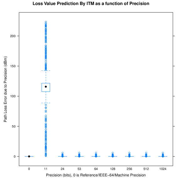
(a) All Precisions

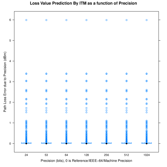
(b) Single-Precision and Greater

Figure 2: Box and whiskers plot of error as a function of precision. The zero-bit case is the machine-precision reference implementation.

3 Results

Figure 2a shows the overall results of this experiment: the error ($\epsilon$) between the multiprecision prediction and the machine precision prediction is plotted. Half-precision arithmetic (11 bits of mantissa, 16 bits total) produces results that vary wildly. Above this, however, beginning at single precision (23 bits of mantissa, 1 bit of sign, 32 bits total), the two programs make very similar predictions. Figure 2b provides a more detailed picture of these remaining cases. Much of the small error is negligible as it is presumably a function of differences in rounding. In the results, there is one clear outlier that produces a 6 dB difference. We investigated this case and found that it was the result of a difference in a branching decision that chooses whether or not to make a particular correction. It is not clear that one direction down the branch offers a better prediction than another, so this case can be safely ignored.

Finally, we investigated the performance, in terms of running time, for the various precisions (on an otherwise unloaded machine). The multiprecision version is not substantially slower than the machine precision implementation—nearly all precisions take the same amount of time to run. At each precision, there are some number of outliers, which require slightly more time, but it is not clearly a function of precision. Hence, if it were the case that the multiple precision implementation was also safer, then its use would be clearly preferable.

4 Conclusions

Although it is not possible to extrapolate universally from these results, they demonstrate that the ITM is not substantially unstable for typical problems and reasonably precise numeric types (i.e., single and double precision IEEE formats). An analytical investigation of stability would go a long way to determine the stability universally, but is a substantial undertaking that involves the careful dissection of dozens of complex algorithms that combine to create the ITM implementation. A motivated investigator may choose to focus his effort on the knife-edge diffraction approximation algorithm, which is almost certainly the most numerically complex component of the model. For most practical purposes, however, the results presented here are sufficient to justify continued use of this model with the confidence that under typical situations it is not significantly affected by rounding and cancellation errors.

References

- [1] G. Hufford, A. Longley, and W. Kissick, “A guide to the use of the ITS irregular terrain model in the area prediction mode,” NTIA, Tech. Rep. 82-100, 1982.
- [2] A. Longley, “Radio propagation in urban areas,” in Vehicular Technology Conference, 1978. 28th IEEE, vol. 28, march 1978, pp. 503 – 511.
- [3] J. S. Seybold, Introduction to RF Propagation. Wiley Interscience, 2005.
- [4] R. Coudé, “Radio Mobile,” http://www.cplus.org/rmw/english1.html, July 2010.
- [5] J. A. Magliacane, “SPLAT! A Terrestrial RF Path Analysis Application for Linux/Unix,” March 2008. [Online]. Available: http://www.qsl.net/kd2bd/splat.html
- [6] Scalable Network Technologies, “Qualnet,” http://www.scalable-networks.com/products/qualnet/, August 2011.
- [7] OPNET Technologies, Inc., “Opnet,” http://www.opnet.com/, August 2011.
- [8] K. Harrison, S. M. Mishra, and A. Sahai, “How much white-space capacity is there?” in DySPAN’10, 2010.
- [9] M. Zennaro, A. Bagula, D. Gascon, and A. Noveleta, “Planning and deploying long distance wireless sensor networks: The integration of simulation and experimentation,” in Ad-Hoc, Mobile and Wireless Networks, ser. Lecture Notes in Computer Science, I. Nikolaidis and K. Wu, Eds. Springer Berlin / Heidelberg, 2010, vol. 6288, pp. 191–204. [Online]. Available: http://dx.doi.org/10.1007/978-3-642-14785-2_15
- [10] C. Martin, the Commissioners Copps, Adelstein, McDowell, and Tate, “In the matter of unliscensed operation in the TV broadcast bands. additional spectrum for unlicensed devices below 900 MHz and in the 3 GHz band.” FCC, Tech. Rep. FCC 08-260, 2008.
- [11] ITU-R, “Prediction procedure for the evaluation of microwave interference between stations on the surface of the earth at frequencies above about 0.7 ghz,” ITU, Tech. Rep. P.452, 2007.
- [12] G. Hufford, “The ITS irregular terrain model, version 1.2.2, the algorithm,” http://flattop.its.bldrdoc.gov/itm.html.
- [13] “The GNU MPFR Library,” http://www.mpfr.org/, June 2010.
- [14] “The GNU Multiple Precision Arithmetic Library,” http://gmplib.org/, June 2010.
- [15] “MPC,” http://www.multiprecision.org/, June 2010.
- [16] T. O. S. G. Foundation, “Geospatial Data Abstraction Library (GDAL),” http://www.gdal.org/.