Tidal Waves a non-adiabatic microscopic description of the yrast states in near-spherical nuclei

Abstract

The yrast states of nuclei that are spherical or weakly deformed in their ground states are described as quadrupole waves running over the nuclear surface, which we call ”tidal waves”. The energies and E2 transition probabilities of the yrast states in nuclides with $Z$= 44, 46, 48 and $N=56,~{}58,~{}...,~{}66$ are calculated by means of the cranking model in a microscopic way. The nonlinear response of the nucleonic orbitals results in a strong coupling between shape and single particle degrees of freedom.

Nuclei are conventionally classified as as ”rotors” and ”vibrators”: Rotors have a fixed shape that goes round; vibrators execute pulsating vibrations. However this familiar view is incomplete, because the quadrupole surface oscillations are five dimensional. In this work, we make use of the fact that the yrast states of vibrational and transitional nuclei have the very simple structure of a running surface waves, which we suggest calling ”tidal waves”. Since they have a constant deformation in the co-rotating system of coordinates, one can calculate their properties microscopically by means of the cranked mean field theory. A first report of the calculations was given in arXiv , which used a less accurate interpolation.

Figure 1: The two linear zero angular momentum modes of a two dimensional oscillator and the circular maximal angular momentum (”yrast”)mode.

Figure 2: Flow pattern of a wave running about the surface of a drop of ideal liquid (upper left), standing waves (pulsating vibrations) of such a droplet (right), and a rigidly rotating body (lower left).

In order to elucidate the concept, consider a body of mass $D$ moving in two dimensions subject to a central force. If the force is generated by a (massless) wire of length $r$, the mass moves on a circle. The angular momentum $J={\cal J}\omega$ increases linearly with the angular velocity $\omega$ while the moment of inertia ${\cal J}=Dr^{2}$ is constant. The energy $E=\omega^{2}{\cal J}/2=J^{2}/(2{\cal J})$ is quadratic in $\omega$ or $J$. One would classify the system as a rotor. Now consider the vibrator shown in Fig. 2. The mass is subject to the force $\vec{F}=-C\vec{x}$. The two perpendicular linear normal modes $x_{1,2}=r_{1,2}\cos(\Omega t+\delta_{1,2})$ have the same frequency $\Omega=\sqrt{C/D}$. Combining them with the same amplitude $r$ and different phases generates the family of elliptical orbits with the same energy $Cr^{2}$, which corresponds to a vibrational multiplet in the quantal context. If the phase difference $\delta_{1}-\delta_{2}=0,\pi$, the orbits are linear oscillations carrying no angular momentum. If $\delta_{1}-\delta_{2}=\pm\pi/2$, the orbits are circles with radius $r$. They carry the maximal angular momentum $J=Dr^{2}\Omega$ for the given energy of $E=Cr^{2}=\Omega J$, that is, they are ”yrast”. One may view the yrast orbits in an alternative way. The mass moves with the angular velocity $\Omega$ on a circular orbit. As in the case of the rotor, the centrifugal force $\vec{x}D\Omega^{2}$ is balanced by the centripedal force $\vec{F}$. In the case of $\vec{F}=-\vec{x}C$ this is only possible if $\Omega=\sqrt{C/D}$, which is independent of $r$. That is, the vibrator and the rotor have the same yrast orbits, the circular motion. The difference is the relation between $E,~{}J,$ and $\omega$. In the case of the rotor, the moment of inertia ${\cal J}=Dr^{2}$ is constant. $E$ and $J$ increase due to the increase $\omega$, resulting in the quadratic relation $E=J^{2}/2{\cal J}$. In the case of the vibrator $\omega=\Omega$ is constant. $E$ and $J$ increase due to an increase of ${\cal J}$ (or equivalently of the radius $r$), resulting in the linear relation $E=\Omega J$. In the general case of a centripedal force $\vec{F}=-\nabla V(|\vec{x}|)$ the yrast orbit is also a circle. Its radius $r_{0}$ is found by minimizing the energy $E(r)=J^{2}/2{\cal J}(r)+V(r)$ with respect to $r$ at fixed angular momentum $J$.

The case of nuclei is completely analogous. Consider the classical motion of the collective quadrupole modes of the nuclear surface described in the framework of the phenomenological Bohr Hamiltionian BMII . Solving the classical equations of motion for the deformation parameters $\alpha_{\mu}(t)$, one finds that the solution with maximal angular momentum for given energy (yrast mode) is a uniform rotation about the axis (z-) with the largest moment of inertia, and static deformation parameters $\beta_{e}$ and $\gamma_{e}$.

$$R(t)=R_{0}[1+\beta_{e}\cos\gamma_{e}Y_{20}(\vartheta)+\sqrt{2}\beta_{e}\sin\gamma_{e}\cos(2\varphi-2\omega t)Y_{22}(\vartheta,\varphi=0)].$$ (1)

The deformation parameters $\beta_{e},\gamma_{e}$ are the equilibrium values corresponding to the minimum of the energy

$$E(J,\beta,\gamma)=\frac{J^{2}}{2{\cal J}(\beta,\gamma)}+V(\beta,\gamma),~{}~{}{\cal J}=4D\beta^{2}\sin^{2}(\gamma)$$ (2)

at given angular momentum $J={\cal J}_{3}\omega$, where $\omega=dE/dJ$.

In the case of harmonic vibrator $V=C\beta^{2}/2$. Minimizing the energy (2), one finds $\gamma_{e}=\pi/2,~{}\beta^{2}_{e}=J/(2\sqrt{DC})$. The energy becomes $E=\omega J=\Omega J/2.$ The wave travels with an angular velocity being one half of the oscillator frequency $\Omega$. The angular momentum grows due to the increase of $\beta_{e}$ which increases moment of inertia ${\cal J}=4D\beta^{2}_{e}=J/(2\sqrt{DC})$. The increase of deformation is reflected by the reduced transition probability $B(E2)\propto\beta_{e}^{2}\propto J$. We suggest calling this mode a ”tidal wave” because it looks like the tidal waves on the oceans of our planet. Fig. 2 upper left illustrates the motion of the surface and shows the stream lines. The right part shows that the running wave of the five-dimensional quadrupole oscillator can be seen as the combination of two standing waves pulsating with a phase shift of $\pi/2$. The standing waves carry no angular momentum. In the case of the quantized oscillator, the $n$ -phonon states form a multiplet. Within the multiplet, the tidal wave represents the state with maximal angular momentum $I=2n$ and the standing wave the state with zero angular momentum $I=0$. The latter is usually invoked in the context of a vibrator (V) - like nucleus.

The analogy with real tidal waves has the caveat that water is not an ideal liquid. The oceans carry damped surface waves, which in their stationary state oscillate with the frequency of the driving gravitational force. The surface wave on the droplet of ideal nuclear liquid runs with an angular velocity corresponding to the natural frequency of the undamped vibrator.

The uniform rotation of a statically deformed shape (1) is the yrast mode for any potential $V(\beta,\gamma)$. If $V$ has a pronounced minimum at $\beta_{0}$ and $\gamma_{0}$ then $\beta_{e}\approx\beta_{0}$ and $\gamma_{e}\approx\gamma_{0}$. The moment of inertia ${\cal J}\approx const.$ and $J\propto\omega$. We refer to this case as a rotor (R). We classify the yrast states of V- like nuclei as ”tidal waves”: The deformation strongly increases with $J$ while $\omega$ stays nearly constant. For the R-like nuclei the deformation stays nearly constant while $J\propto\omega$. The transition between the V and R regimes is gradual.

The left part of Fig. 2 illustrates that same uniform rotation of the surface may be generated in different ways, by the irrotational flow of an ideal liquid or by rigid rotation. Yet, the flow pattern of real nuclei differs from both of these ideal cases. It must be calculated in a microscopic way, which can be achieved by finding the selfconsistent mean field solution in a rotating frame of reference. We use the cranking model for calculating the tidal wave modes in vibrational and transitional nuclei. Marshalek marshalek demonstrated that the RPA equations for harmonic quadrupole vibrations of nuclei with a spherical ground state are a solution to the selfconsistent cranking model if the deformation of the mean field is treated as a small perturbation. In this paper we solve numerically the cranking problem without the small deformation approximation, which allows us to describe the yrast states of all nuclei in the range between the harmonic vibrators and rigid rotors. Such microscopic approach takes into account not only the quadrupole shape degrees of freedom, as in the above discussed phenomenological model, but also the the quasiparticle degrees of freedom, which play an important role to be discussed below. Of course, the cranking model also applies to the rotational nuclei.

We use the Shell Correction version of the Tilted Axis Cranking model (SCTAC) in order to study the tidal waves in the nuclides with $Z=$44, 46, 48 and $N=$56, 58, 60, 62, 64, 66. The details and parameters of SCTAC are described in Ref.qptac . For the yrast states of even-even nuclei, the axis of rotation coincides with a principal axis (x). The condition $<J_{x}>=J=I$ is used to fix $\omega$, which is solved numerically for each point on a grid in the $\varepsilon_{2}-\gamma$ plane. In solving it is crucial to employ the diabatic tracing technique described in Ref.qptac , which is illustrated in Fig. 3.

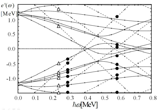
Figure 3: The Quasi Neutron Routhians for $N=56$ and $\varepsilon_{2}=0.13$, $\gamma=0$. Full lines: positive parity, dash dotted lines: negative parity (h_11/2). The full circles show the g-configuration, which corresponds to a tidal wave, the open triangles show the s-configuration.

The interpolated function $E(\varepsilon_{2},\gamma,J)$ is minimized with respect to the deformation parameters for fixed angular momentum. The final value of $\omega(J)$ for the equilibrium deformation is found by interpolation between the values at the grid points. It is shown as the theoretical points in the Figure 5. It is noted, that the standard technique of finding the selfconsistent solutions by iteration at fixed $\omega$ becomes problematic for tidal waves close to the harmonic limit because the total Routhian is nearly deformation independent. The pairing parameters are kept fixed to $\Delta_{n}=\Delta_{p}=1.1$ MeV, and the chemical potentials are $\lambda$ adjusted to the particle numbers at $\omega=0$. We slightly correct $J(\omega)=J_{SCTAC}(\omega)+100MeV^{-1}\varepsilon_{2}^{2}\sin^{2}(\gamma-\pi/3)\omega,$ which adds less than 0.5 $\hbar$ to the angular momentum. About half of it takes into account the coupling between the oscillator shells and another half is expected to come from quadrupole pairing, both being neglected in SCTAC. The changes due to the correction are smaller than the radius of the open circles in Figs. 5 and 6.

The $B(E2,I->I-2)$ values are calculated for $J=I$ as described in qptac for $\theta=90^{o}$, which is the high-spin limit. In addition we give the values multiplied by the factor $I(I-1)/(I+1/2)(I-1/2)$, which corrects for the low-spin deviation of the $B(E2)$ values from the high-spin limit in the case of an axial rotor. For vibrators, the correction factor should not be applied marshalek , for rotors it should. The correction factor accounts for zero point fluctuations of the angular momentum of a rigid axial rotor. Since the present approach does not take into account the zero point motion of the collective variables in a systematic way, one should consider the two values in Fig. 6 as limits, between which the $B(E2)$ values lie.

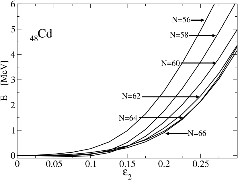
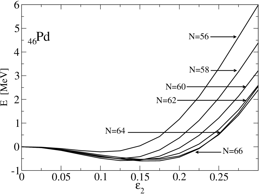
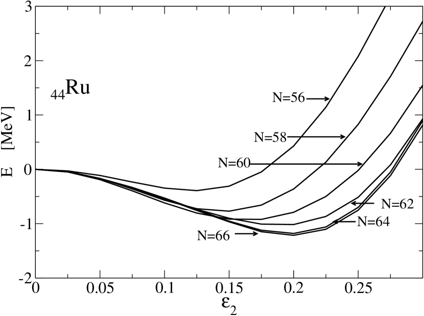
Figure 4: The ground state energies at $\gamma=5^{\circ}$.

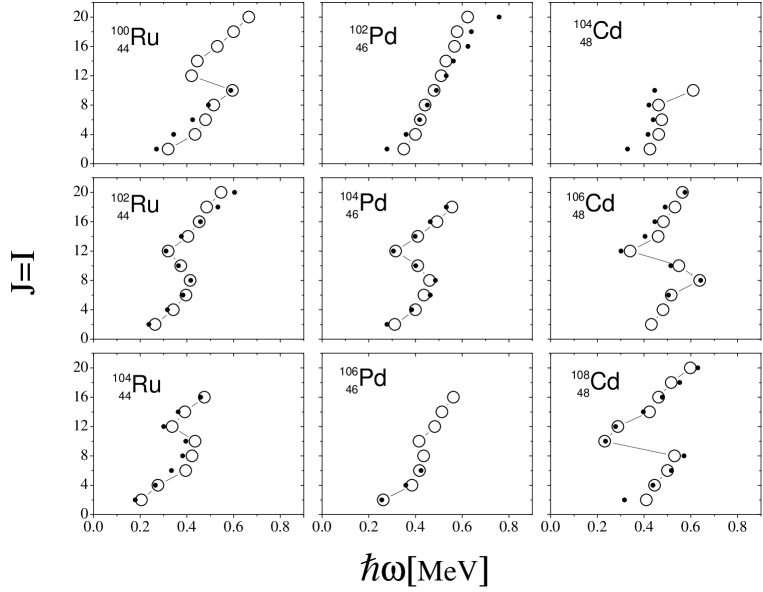
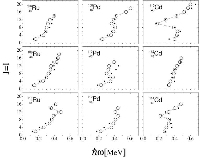
Figure 5: Angular momentum $J$ as function of the angular frequency $\omega$ in the mass 110 region. Full circles show the experiment, open the calculations. The experimental functions $J(\omega)$ and ${\cal J}(I)$ are defined in the standard way by as $\omega(I)=(E(I)-E(I-2))/2,$ $J(I)=I-1/2$, ${\cal J}(I)=J(I)/\omega(I)$. Data fromensdf .

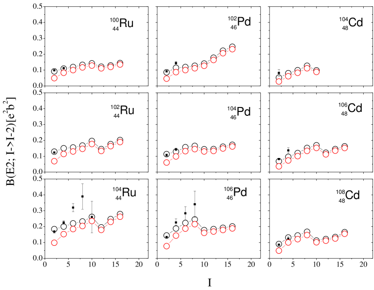
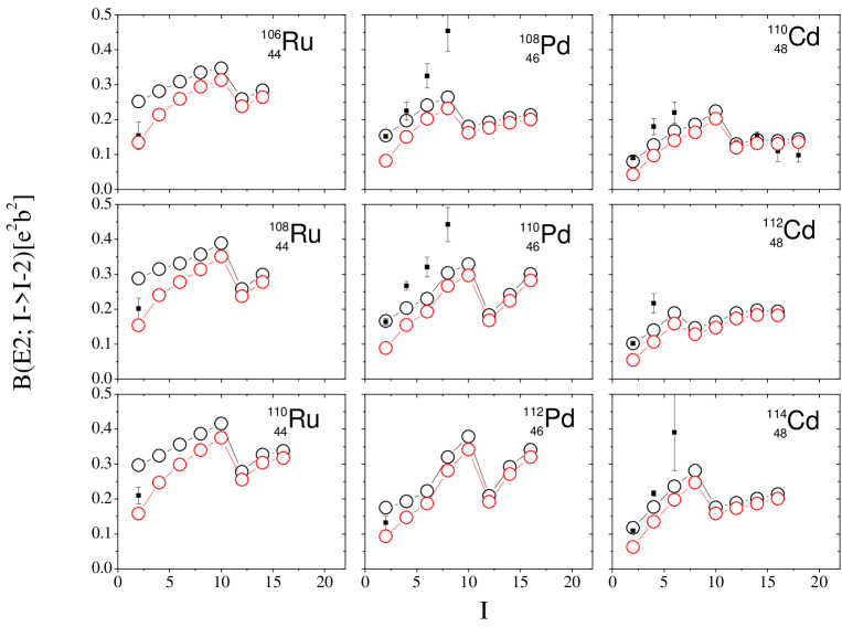
Figure 6: The $B(E2,I->I-2)$ values in the mass 110 region. Full squares show the experiment, open circles the calculations. The higher circles (black) are the high-spin limit, the lower circles (red) include the low-spin correction factor (see text). The $B(E2)$ values lie between the two values, where V-like nuclei are expected closer to the higher values and R-like nuclei closer to the lower values. Data from raman ; ensdf .

The ground state energies are shown in Fig. 4. They are calculated using the modified oscillator potential with the parameters given in Ref. qptac , adding a small adjustment $k\varepsilon_{2}^{2}$ with $k=$8.5, 7.9, 8.5, 9.6, 11.9, 14.5 MeV for $N$= 56, 58, 60, 62, 64, 66, respectively. The correction term slightly disfavors deformation. It is substantially smaller than the differences between deformation energies calculated from the various mean field theories used at present. The tendency to deformation increases with the numbers of valence proton holes and valence neutron particles in the $Z=N=50$ shell. The $Z=48$ isotopes are spherical, becoming softer with increasing $N$. The $Z=44$ isotopes are slightly deformed, very soft, becoming less soft with $N$. The $Z=46$ isotopes are intermediate. The equilibrium deformations for $2\leq I$ are $\gamma_{e}=0^{\circ}$ and $0.1<\beta_{e}<0.2$, except ^110,112Cd for which $\gamma=10^{\circ}$ - $15^{\circ}$ for $2\leq I\leq 8$. The heavy Pd isotopes have a larger $\beta_{e}$. Figs. 5 and 6 compare the calculated values of $\omega(J)$ and $B(E2,I->I-2)$ with experiment. The calculated frequencies reproduce the experimental ones very well. The calculated $B(E2)$ in the V-like nuclei increase somewhat slower with $I$ than in experiment. The back-bend in the $J(\omega)$ curves is caused by the rotational alignment of a pair of $h_{11/2}$ neutrons (change from the g-configuration to the s- configuration in Fig. 3). The sharpness of the alignment depends sensitively on the position of the neutron chemical potential $\lambda_{n}$ relative to the $h_{11/2}$ levels Hamamoto , which explains why there is a strong back-bend for some $N$ and only a smooth up-bend for other $N$. The $h_{11/2}$ levels move with the changing deformation, and differences of the deformation are the reason why $J(\omega)$ sharply back-bends in $Z=48,~{}N=62$ while it gradually grows in $Z=44,~{}N=62$. Also normal parity neutron orbitals contribute to the $J(\omega)$ in a non-linear way, in particular at the avoided crossings between them (around $\hbar\omega=$ 0.53 MeV in Fig. 3). For example, they are responsible that in ¹¹⁰Cd the point $I=8$ has a lower $\omega$ than the point $I=6$. The large frequency encountered at small deformation makes also other orbitals than the high-j intruders react in a non-linear way to the inertial forces. For many nuclides the quasiparticle degrees cannot be treated in a perturbative way for $I\geq 6$, which means the separation of the collective quadrupole degrees of freedom becomes problematic. For the nuclei with the smallest numbers of valence particles and holes this entanglement of collective and single particle degrees appears already for $I=4$, which is reflected by the irregular curves $J(\omega)$ for $Z=48,~{}N=56$ in Fig. 5.

As seen in Fig. 6, the aligned $h_{11/2}$ quasi neutrons stabilize the deformation at a smaller value than reached before, which is reflected by the decrease of the $B(E2)$ values. The deformation increases slower than before the alignment, which means the motion becomes more rotational. In some cases, the alignment process is extended over several units of angular momentum, keeping $\omega$ nearly constant. This means the simple picture of tidal waves, as running at nearly constant angular velocity and gaining angular momentum by deforming does not account for the full complexity of real nuclei. The single particle degrees of freedom also provide their share of angular momentum, such that the rotational frequency remains constant.

¹⁰²Pd is a special case. The g- and s-configurations do not mix, and are both observed up to $I=20$. Figs. 5 and 6 show only the g-sequence, which represents a tidal wave that gains angular momentum predominantly by increasing the deformation, as discussed above for the droplet model. Its $I=16$ state corresponds to eight stacked phonons! Only for $I>16$ the alignment of the positive parity neutrons (avoided crossing at $\hbar\omega\approx 0.53$ MeV in Fig. 3) becomes a comparable source of angular momentum.

In conclusion, the yrast states of vibrational and transitional nuclei can be understood as tidal waves that run over the nuclear surface, which have a static deformation, the wave amplitude, in the frame of reference co-rotating with the wave. In contrast to rotors, most of the angular momentum is gained by an increase of the deformation while the angular velocity increases only weakly. Since tidal waves have a static deformation in the rotating frame, the rotating mean field approximation (Cranking model) provides a microscopic description. The yrast states of “spherical” or weakly deformed nuclei with $44\leq Z\leq 48,~{}56\leq N\leq 66$ were calculated up to spin 16. These microscopic calculations reproduce the energies and electromagnetic $E2$ transition probabilities in detail. The structure of the yrast states turns out to be complex. The shape degrees of freedom and the single particle degrees of freedom are intimately interwoven. The non-linear response to the inertial forces of the individual orbitals at the Fermi surface determines the way the angular momentum is generated. This lack of separation of the collective motion from the single particle becomes increasingly important for increasing angular momentum and decreasing number of valence nucleons.

Supported by the DoE Grant DE-FG02-95ER4093.

References

- (1) S. Frauendorf, Y. Gu, and J. Sun, arXiv-id: 0709.0254 (2007)
- (2) A. Bohr and B. R. Mottelson, Nuclear Structure, Vol. II (Benjamin, New York, 1975).
- (3) ENSDF data bank, http://www.nndc.bnl.gov
- (4) E.R. Marshalek, Phys. Rev. C 54 159 (1996).
- (5) S. Frauendorf, Nucl. Phys. A 677, 115 (2000).
- (6) S. Raman et al., Atomic D. and Nucl. D. Tab. 78, 1 (2001)
- (7) R. Bengtsson, et al., Phys. Lett. B 73, 259 (1978)