Star formation at $\bf z=1.47$ from HiZELS: An H$\alpha$+[Oii] double-blind study

Abstract

This paper presents the results from the first wide and deep dual narrow-band survey to select H$\alpha$ and [Oii] line emitters at $z=1.47\pm 0.02$, exploiting synergies between the United Kingdom InfraRed Telescope and the Subaru telescope by using matched narrow-band filters in the $H$ and $z^{\prime}$ bands. The H$\alpha$ survey at $z=1.47$ reaches a 3 $\sigma$ flux limit of F${}_{{\rm H}\alpha}\approx 7\times 10^{-17}$ erg s^-1 cm^-2 (corresponding to a limiting SFR in H$\alpha$ of $\approx 7$ M_⊙ yr^-1) and detects $\approx 200$ H$\alpha$ emitters over $0.7$ deg², while the much deeper [Oii] survey reaches an effective flux of $\approx 7\times 10^{-18}$ erg s^-1 cm^-2 (SFR in [Oii] of $\sim 1$ M_⊙ yr^-1), detecting $\approx 1400$ $z=1.47$ [Oii] emitters in a matched co-moving volume of $\sim 2.5\times 10^{5}$ Mpc³. The combined survey results in the identification of 190 simultaneous H$\alpha$ and [Oii] emitters at $z=1.47$. H$\alpha$ and [Oii] luminosity functions are derived and both are shown to evolve significantly from $z\sim 0$ in a consistent way. The star formation rate density of the Universe at $z=1.47$ is evaluated, with the H$\alpha$ analysis yielding $\rho_{\rm SFR}=0.16\pm 0.05$ M_⊙ yr^-1 Mpc^-3 and the [Oii] analysis $\rho_{\rm SFR}=0.17\pm 0.04$ M_⊙ yr^-1 Mpc^-3. The measurements are combined with other studies, providing a self-consistent measurement of the star formation history of the Universe over the last $\sim 11$ Gyrs. By using a large comparison sample at $z\sim 0.1$, derived from the Sloan Digital Sky Survey, [Oii]/H$\alpha$ line ratios are calibrated as probes of dust-extinction. H$\alpha$ emitters at $z\sim 1.47$ show on average A${}_{\rm H\alpha}\approx 1$ mag, the same as found by SDSS in the local Universe. It is shown that although dust extinction correlates with SFR, the relation evolves by about $\sim 0.5$ mag from $z\sim 1.5$ to $z\sim 0$, with local relations over-predicting the dust extinction corrections at high-$z$ by that amount. Stellar mass is found to be a much more fundamental extinction predictor, with the same relation between mass and dust-extinction being valid at both $z\sim 0$ and $z\sim 1.5$, at least for low and moderate stellar masses. The evolution in the extinction-SFR relation is therefore interpreted as being due to the evolution in median specific SFRs over cosmic time. Dust extinction corrections as a function of optical colours are also derived and shown to be broadly valid at both $z\sim 0$ and $z\sim 1.5$, offering simpler mechanisms for estimating extinction in moderately star-forming systems over the last $\sim 9$ Gyrs.

1 Introduction

It is now clear that the “epoch” of galaxy formation occurs at $z>1$, as surveys measuring the star formation rate density ($\rho_{\rm SFR}$) as a function of epoch show that $\rho_{\rm SFR}$ rises steeply out to $z\sim 1$ (e.g. Lilly et al., 1996; Hopkins & Beacom, 2006), but determining the redshift where $\rho_{\rm SFR}$ peaked at $z>1$ is more difficult.

Accurately determining $\rho_{\rm SFR}$ requires the selection of clean and well-defined samples of star-forming galaxies over representative volumes. In practice, such selection is done by detecting signatures of massive stars (being very short-lived, their presence implies recent episodes of star formation). The high luminosities of such massive stars allow them to be traced up to very high redshift, and to estimate star formation rates (SFRs). Such stars emit strongly in the ultra-violet (UV), and although this is often significantly absorbed, it is then re-emitted through a variety of processes, resulting in detectable signatures such as strong emission lines or thermal infra-red emission from heated dust (see discussion in Hopkins et al., 2003). Ideally, the use of different tracers of recent star formation would provide a consistent view, but in reality, because they have different selection biases, and require different assumptions/extrapolations, measurements are often significantly discrepant (e.g. Hopkins & Beacom, 2006). A major issue is the difficulty and uncertainty in correcting for (dust) extinction, especially for UV and optical wavelengths, leading to large systematic uncertainties (and potentially missing entire populations). An additional complication comes from surveys at different epochs making use of different indicators due to instrumentation and detection limitations. For example, while for $0<z~{}\lower 2.15277pt\hbox{$\buildrel<\over{\sim}$}~{}0.4$ the evolution of $\rho_{\rm SFR}$ is typically estimated using H$\alpha$ luminosity, because it is easily targeted in the optical (e.g. Ly et al., 2007; Shioya et al., 2008; Dale et al., 2010), at higher redshifts the line is redshifted into the near-infrared, and [Oii] 3727 – hereafter [Oii] – luminosity (much more affected by extinction than H$\alpha$, and also a metallicity-dependent indicator) is used instead (e.g. Zhu et al., 2009; Bayliss et al., 2011).

The [Oii] emission line can be traced in the optical window up to $z\sim 1.5$ and many authors have attempted to measure the evolution of [Oii] luminosity function up to such look-back times (e.g. Teplitz et al., 2003; Hogg et al., 1998; Gallego et al., 2002; Takahashi et al., 2007; Zhu et al., 2009). Such studies have identified a strong evolution from $z=0$ to $z>1$ (e.g. Gallego et al., 2002; Zhu et al., 2009), although the evolution seems to be slightly different from that seen in the H$\alpha$ luminosity function. Part of the differences may well arise from the difficulty in using [Oii] luminosity density directly as a star-formation rate density indicator: [Oii] luminosity is calibrated locally using H$\alpha$ (see e.g. Aragón-Salamanca et al., 2003; Mouhcine et al., 2005, for a comparison between both emission-lines at low-$z$), but the actual calibration depends on metallicity and dust-extinction (c.f. Jansen et al., 2001; Kewley et al., 2004). These issues have been reported by many studies, mostly using data from the local Universe or low redshift (see e.g. Gilbank et al., 2010, for a comparison between both lines and other indicators in the Sloan Digital Sky Survey), for which it is possible to measure both H$\alpha$ and [Oii]. However, so far it has not been possible to directly compare the H$\alpha$ and [Oii] indicators at $z>1$ using large-enough samples to test, extend and improve our understanding.

While some H$\alpha$ studies beyond $z\sim 0.4$ have been conducted in the 90’s (e.g. Bunker et al., 1995; Malkan et al., 1995), tracing the H$\alpha$ emission line in the infrared, the small field-of-view of infrared detectors at that time made it very hard to detect more than $\sim 1-2$ emitters at $z>1$ (e.g. van der Werf et al., 2000) using ground-based narrow-band surveys. Slitless spectroscopy using NICMOS on the Hubble Space Telescope (HST) provided a space-based alternative to make significant progress, particularly by allowing much deeper observations than those from the ground (e.g. McCarthy et al., 1999; Yan et al., 1999; Hopkins et al., 2000). Further progress is now being obtained with WFC3 on HST, as recent studies (e.g. Atek et al., 2010; Straughn et al., 2011; van Dokkum et al., 2011) take advantage of the increased sensibility and the wider field-of-view (although still relatively small when compared to wide-field ground-based infrared detectors) of WFC3 to simultaneously look for fainter emitters and increase the sample sizes. Furthermore, the development of wide-field near-infrared cameras in the last decade has finally made it possible to conduct ground-based large area H$\alpha$ surveys (necessary to overcome cosmic variance) which can look for such emission-line galaxies all the way up to $z\approx 2.5$.

HiZELS, the High-redshift(Z) Emission Line Survey (Geach et al., 2008; Sobral et al., 2009a, hereafter S09) is a Campaign Project using the Wide Field CAMera (WFCAM) on the United Kingdom Infra-Red Telescope (UKIRT) and exploits specially-designed narrow-band filters in the J and H bands (NB_J and NB_H), along with the H₂S1 filter in the K band, to undertake panoramic, moderate depth surveys for line emitters. HiZELS is primarily targeting the H$\alpha$ emission line redshifted into the near-infrared at $z=0.84$, $z=1.47$ and $z=2.23$. The main HiZELS survey aims to cover $\approx 7$ deg² (to overcome cosmic variance) and is detecting $\sim 1000$ emitters over volumes of $>10^{6}$ Mpc³ with each filter, reaching limiting H$\alpha$ (observed) SFRs of $\approx 3$, $6$ and $30$ M_⊙ yr^-1 at $z=0.84$, $z=1.47$ and $z=2.23$. Such data will pin down the likely peak of $\rho_{\rm SFR}$ and provide detailed information about the population of star-forming galaxies at each epoch (see Best et al., 2010).

HiZELS provides precise measurements of the evolution of the H$\alpha$ luminosity function from $z=0.0$ to $z=2.23$ (Geach et al. 2008; S09), while the contribution from much deeper H$\alpha$ surveys over smaller areas (e.g. Hayes et al., 2010; Ly et al., 2011) offers the possibility of also exploring the faint-population. The H$\alpha$ luminosity function evolves significantly, mostly due to an increase by more than one order of magnitude in L${}_{\rm H\alpha}^{*}$ (S09), the characteristic H$\alpha$ luminosity, from the local Universe to $z=2.23$. In addition, Sobral et al. (2011) found that at $z=0.84$ the faint-end slope of the luminosity function is strongly dependent on the environment, with the H$\alpha$ luminosity function being much steeper in low density regions and much shallower in the group/cluster environments. Whether this is also found at higher redshifts remains unknown.

Figure 1: A comparison between the NB_H redshift coverage of the H$\alpha$ emission line and the NB921 redshift coverage of the [Oii] emission-line, revealing that the two filters are extremely well matched and ideal for a dual H$\alpha$-[Oii] narrow-band survey. The [Oii] coverage is only slightly wider (in redshift) than the H$\alpha$ coverage – but this is shown to have little to no effect on the analysis (c.f. Section 4.5).

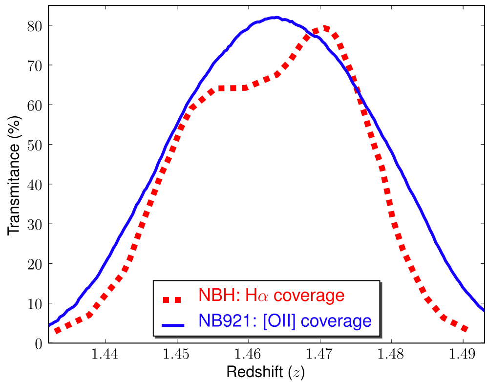
Indeed, while it is now possible to detect H$\alpha$ emission over very wide areas up to $z>2$, distinguishing between H$\alpha$ and any other emission line at any redshift is a challenge, particularly over large areas where it is unfeasible to assemble ultra-deep multi-wavelength data over dozens of bands. Matched dual narrow-band surveys offer a solution to the problem; in particular, since the NB921 narrow-band filter on Subaru is able to probe the [Oii] emission line for the same redshift range ($z\sim 1.47$) as the HiZELS narrow-band $H$ filter on UKIRT probes H$\alpha$ (see Figure 1), a matched and sufficiently deep survey would not only provide a simple, clean selection ($z=1.47$ sources will be detected as emitters in both data-sets), but also provide a means of directly comparing H$\alpha$ and [Oii] at $z\sim 1.5$ for large samples for the first time.

Table 1: Observation log for the NB_H observations of the UDS field, taken using WFCAM on UKIRT, during 2008, 2009 and 2010. Limiting magnitudes (3 $\sigma$) are the average of the four frames which constitute a field, based on the the measurements of 10⁶ randomly placed 2^′′ apertures in each frame. Integration times given in brackets present the total integration times obtained at the telescope prior to rejection of data taken in poorer conditions (see §2.1).

Field	R.A.	Dec.	Int. time	FHWM	Dates	$m_{lim}$ NBH(Vega)
	(J2000)	(J2000)	(ks)	(′′)		(3$\sigma$)
UKIDSS-UDS NE	02 18 29	$-$04 52 20	18.2 (18.2)	0.8	2008 Sep 28-29; 2009 Aug 16-17; 2010 Jul 22	21.2
UKIDSS-UDS NW	02 17 36	$-$04 52 20	17.1 (18.3)	0.9	2008 Sep 25, 29; 2010 Jul 18, 22	20.9
UKIDSS-UDS SE	02 18 29	$-$05 05 53	28.0 (28.0)	0.8	2008 Sep 25, 28-29; 2009 Aug 16-17	21.4
UKIDSS-UDS SW	02 17 38	$-$05 05 34	18.3 (19.1)	0.8	2008 Oct-Nov; 2009 Aug 16-17; 2010 Jul 23	21.2

This paper presents deep narrow-band imaging using the NB_H filter at $\lambda=1.617\mu$m, as part of HiZELS, over $0.79\deg^{2}$ in the UKIDSS Ultra Deep Survey (Lawrence et al., 2007) field (UDS) and combines the data with ultra-deep NB921 imaging taken using Suprime-Cam on the Subaru telescope, to explore an extremely well-matched H$\alpha$-[Oii] narrow-band survey over $0.70\deg^{2}$.

The paper is organised as follows: §2 presents the observations, data reduction, source extraction and catalogue production. In §3, emission-line galaxies are selected and, using colours and photometric redshifts, the samples of H$\alpha$ and [Oii] selected $z=1.47$ emitters are presented. §4 presents the H$\alpha$ and [Oii] luminosity functions and the derived star-formation rate density at $z=1.47$, together with an accurate measurement of their evolution. In §5, the large sample of robust H$\alpha$-[Oii] emitters is used to conduct line ratio studies and compare these with a large sample selected locally from the Sloan Digital Sky Survey (SDSS). These are used to investigate the extinction properties of the galaxies, and how these evolve with redshift. Finally, §6 outlines the main conclusions. An H${}_{0}=70$ km s^-1 Mpc^-1, $\Omega_{M}=0.3$ and $\Omega_{\Lambda}=0.7$ cosmology is used. Magnitudes are in the Vega system, except if noted otherwise.

2 DATA AND SAMPLES

2.1 Near-infrared NB_H imaging with UKIRT

The UKIDSS UDS field was observed with WFCAM on UKIRT using a set of custom narrow-band $H$ filters (NB_H, $\lambda=1.617\,\mu$m, $\Delta\lambda=0.021\,\mu$m), as detailed in Table 1. WFCAM’s standard “paw-print” configuration of four $2048\times 2048$ ($0.4^{\prime\prime}$ pixel^-1) detectors offset by $\sim 20^{\prime}$ was macrostepped four times to cover a contiguous region of $\sim 55^{\prime}\times 55^{\prime}$ (Casali et al., 2007), with individual narrow-band exposures of 100 s. The conditions were mostly photometric. The Non Destructive Read (NDR) mode was used for all narrow-band observations to minimise the effects of cosmic rays in long exposures. The observations were obtained by jittering around 14 different positions in each of the 4 pointings. The UKIDSS UDS $H$-band image (24 AB, 5$\sigma$) overlaps entirely with the full narrow-band image, yielding a total survey area of $0.79\deg^{2}$.

A dedicated pipeline has been developed for HiZELS (PfHiZELS, c.f. S09 for more details), and was used to fully reduce the data. Very briefly, the pipeline dark-subtracts the data and median combines dark-subtracted data (without offsetting) to obtain a first-pass flat field for each jitter pattern. The latter is used to produce a badpixel mask for each chip by flagging pixels which deviate by more than $5\sigma$ from the median value. Frames are individually flattened and individual source masks are produced for each frame. A new final flat is then created masking detected sources (for each jitter pattern) and all data are flattened. A world coordinate system is fitted to each frame by querying the USNO A2.0 catalogue (typically $\sim 70-80$ stars per frame). Finally, all individual reduced frames were visually inspected, resulting in the rejection (for each of the four cameras) of 12 frames for the NW field and 8 frames in the SW field due to bad quality (FWHM$>1.1^{\prime\prime}$ or $A_{H}>0.25$ mag). Final frames which passed the data-control were de-jittered and median co-added with SWarp (Bertin 1998), including a background mesh-based sky subtraction optimized for narrow-band data, and masking of bad-pixels and cosmic-rays. It should be noted that WFCAM frames suffer from significant cross-talk artifacts (toroidal features at regular pixel intervals from bright sources in the read-out direction); because these are linked to a “physical” location, they can only be removed from the source catalogue (see §2.2).

Narrow-band images were photometrically calibrated (independently) by matching $\sim 70$ stars with $m_{H}=11-16$ per frame from the 2MASS All-Sky catalogue of Point Sources (Cutri et al., 2003) which are unsaturated in the narrow-band frames.

2.2 NB_H Source Extraction and Survey Limits

Sources were extracted using SExtractor (Bertin & Arnouts, 1996). Photometry was measured in apertures of $2^{\prime\prime}$ diameter. In order to clean spurious sources from the catalogue (essential to remove cross-talk artifacts), the final images were visually inspected; this revealed that sources brighter than $\sim 11.5$ mag (NB_H, Vega) were surrounded by a number of artifacts detected within “bright halos”, as well as cross-talk. Fainter sources (up to 16 mag) showed only cross-talk features. Sources fainter than 16 mag did not produce any detectable cross-talk at the depth of the observations. Cross-talk sources and detections in the halo regions were removed from the catalogue separately for each frame, which greatly simplifies their identification.

The average 3 $\sigma$ depth of the entire set of NB_H frames is 21.2 mag; this is measured using a set of 10⁶ randomly placed apertures per frame. Above the 3 $\sigma$ threshold in each frame, the narrow-band imaging detects a total of 23394 sources (5904, 4533, 6946 and 6011 in the NE, NW, SE and SW pointings, respectively) across $0.78\deg^{2}$ (after removal of regions in which cross-talk and other artifacts caused by bright objects are located)

Figure 2: Narrow-band excess as a function of narrow-band magnitude for NB_H (left panel, Vega magnitudes) and NB921 (right panel, AB magnitudes) data. These show $>3\sigma$ detections in narrow-band imaging and the lines present the average 2.5 $\Sigma$ and 3.0 $\Sigma$ colour significances for NB_H and NB921, respectively (for the average depth, but note that the analysis is done individually for each frame). Also, due to the very high number of detected sources in NB921, only 1 in every 5 sources is shown. The horizontal dashed lines present the equivalent width cuts used for NB_H and NB921 data – these correspond to $z=1.47$ rest-frame EW limits of 20 Å for H$\alpha$ and 10 Å for [Oii]. Narrow-band excess sources in both NB_H and NB921 (double-emitters) are shown, and constitute a robust sample of H$\alpha$/[Oii] candidate emitters – see Figure 3 for a visualisation of one such emitters.

2.3 Optical NB921 imaging with Subaru

Archival Subaru/Suprime-Cam NB921 data of the UDS field are available, taken by Ouchi et al. (2009, 2010). The field was observed with Suprime-Cam on Subaru as part of the Subaru/XMM-Newton Deep Survey (SXDS, Ouchi et al., 2008) during 2005–2007. The NB921 filter is centered at 9196 Å with a FWHM of 132 Å, and was used to cover the field with 5 pointings with a total integration of 45.1 hours (individual exposures ranging from 8 to 10 hours) – see Ouchi et al. (2010). The raw NB921 data were downloaded from the archive and reduced with the Suprime-Cam Deep field REDuction package (SDFRED, Yagi et al., 2002; Ouchi et al., 2004) and IRAF. The combined images were aligned to the public $z^{\prime}$-band images of Subaru-XMM Deep Survey (SXDS; Furusawa et al., 2008) and PSF matched (FWHM$=0.8^{\prime\prime}$). The NB921 zero points were determined using $z^{\prime}$ data, so that the $z^{\prime}$-NB921 colour distributions of SXDS would be consistent with that of Subaru Deep Field data (Kashikawa et al., 2004). Source detection and photometry were performed using SExtractor (Bertin & Arnouts, 1996). Sources were detected on each individual NB921 image and magnitudes measured with $2^{\prime\prime}$ diameter apertures. The average NB921 3$\sigma$ limiting magnitude is estimated to be 26.3 (AB) by randomly placing $10^{6}$ 2^′′ apertures in each frame; down to that depth, 347341 sources are detected over the entire 1 deg² area (5 Suprime-Cam pointings). Note that NB921 and $z^{\prime}$ magnitudes are given in the AB system.

3 SELECTION

3.1 Narrowband excess selection

Potential line emitters (NB_H and NB921) are selected according to the significance of their broad-band $-$ narrow-band ($BB-NB$) colour, as they will have $(BB-\,NB)>0$. However, true emitters need to be distinguished from those with positive colours due to the scatter in the magnitude measurements; this is done by quantifying the significance of the narrowband excess. The parameter $\Sigma$ (see S09) quantifies the excess compared to the random scatter expected for a source with zero colour, as a function of narrow-band magnitude (c.f. S09).

Figure 3: The top panels show a strong NB_H emitter, clearly revealed after subtracting the $H$ continuum. The bottom panels show the same sky area ($\sim 30^{\prime\prime}\times 30^{\prime\prime}$) in NB921 and $z^{\prime}$, revealing that the NB_H emitter is also a strong NB921 emitter (and thus a H$\alpha$+[Oii] $z\sim 1.47$ emitter). Note the depth difference, and how non-emitters disappear when the continuum estimated flux is subtracted from the narrow-band flux (other fainter NB921 emitters are also revealed).

Neither of the narrow-band filters falls at the center of the broad-band filters and thus objects with redder colours will tend to have a negative ($H-$ NB_H) colour, and a positive ($z^{\prime}$-NB921) colour, while bluer sources will have ($H-$ NB${}_{\rm H})>0$ and ($z^{\prime}$-NB921$)<0$. This will not only affect the selection of emission line objects, but can also result in an over/under-estimation of emission-line fluxes because it will lead to an under/over-estimation of the continuum. Fortunately, this can be broadly corrected by considering the broad-band colours of each source, as in S09. For the NB_H data, this is done by studying ($H-$ NB_H) as a function of $(J-H)$ colour for all sources detected in the NB_H frames. A linear fit is derived and is used to correct the initial $H$ magnitudes to produce an effective $H^{\prime}$ magnitude appropriate for estimation of the continuum contribution at the wavelength of the NB_H filter. This assures a mean zero ($H^{\prime}-$ NB_H) as a function of ($J-H$), and also results in no significant trend as a function of ($H-K$). The correction is given by:

$$(H^{\prime}-\,\rm NB_{H})=(\it H-\rm NB_{H})-0.1(\it J-H\rm)-0.03.$$ (1)

For the NB921 data, a similar approach is taken, but using $z^{\prime}-J$ colours instead. Colours are corrected by using the best linear fit:

$$(z^{\prime\prime}-\,\rm NB921)=(\it z^{\prime}\rm-NB921)-0.05(\it z^{\prime}-J^{\prime}\rm)+0.15.$$ (2)

Emission line fluxes, F_line, and equivalent widths, EW_line, are computed using:

$${\rm F}_{{\rm line}}=\Delta\lambda_{NB}\frac{f_{NB}-f_{BB}}{1-(\Delta\lambda_{NB}/\Delta\lambda_{BB})}$$ (3)

and

$${\rm EW}_{{\rm line}}=\Delta\lambda_{NB}\frac{f_{NB}-f_{BB}}{f_{BB}-f_{NB}(\Delta\lambda_{NB}/\Delta\lambda_{BB})}$$ (4)

where $\Delta\lambda_{NB}$ and $\Delta\lambda_{BB}$ are the FWHMs of the narrow- and broad-band filters ($211$ Å and $132$ Å for NB_H and NB921; $2893$ Å and $955$ Å for $H$ and $z^{\prime}$, respectively), and $f_{NB}$ and $f_{BB}$ are the flux densities measured for the narrow and broad-bands, respectively. Note that $f_{BB}$ is computed by using the corrected BB^′ magnitudes, which are a much better approximation of the continuum for the present purposes and guarantee that the median flux distribution is zero. Note that the latter formula is only valid because magnitudes and colours have been corrected to guarantee a flux and colour distribution centered at zero.

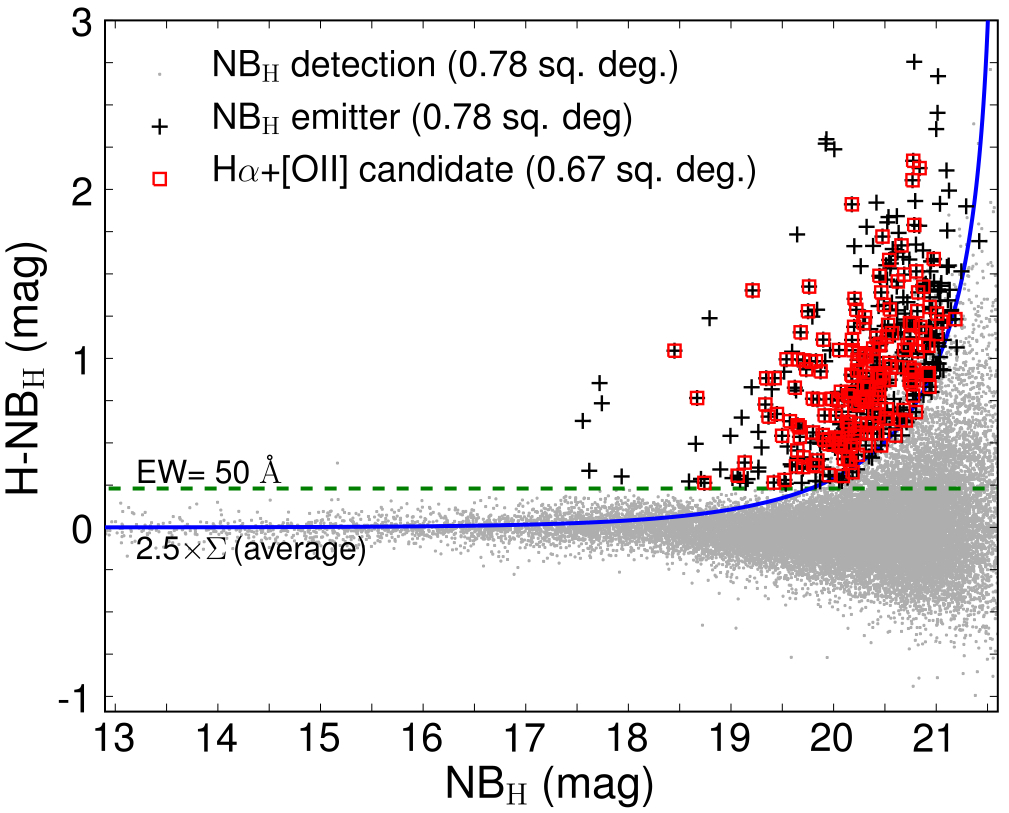
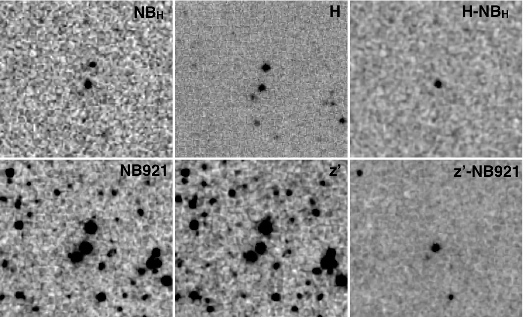
The selection of emission-line candidates is done following S09 (see also Ouchi et al., 2010). Narrow-band sources in the $H$ band (NB_H) are selected as line emitters if they have an individual $>3$ $\sigma$ detection in NB_H and present a colour excess significance of $\Sigma>2.5$ (which broadly corresponds to a flux limit, see S09), and an observed $\rm EW>50$ Å (corresponding to $\rm EW>20$ Å rest-frame for the H$\alpha$ line at $z=1.47$). NB921 sources are selected as potential emitters if they have an individual $>3$ $\sigma$ detection in NB921 and present a colour excess significance of $\Sigma>3.0$ (as the data are much deeper, a higher significance cut can be applied) and EW$>25$ Å (corresponding to $\rm EW>10$ Å for [Oii] emitters at $z=1.47$). The EW cuts are applied to avoid including bright foreground objects with a large significance and a steep continuum across the $H$ or $z^{\prime}$ bands, and were chosen to reflect the general scatter around the zero colour at bright magnitudes (thus the difference between NB_H and NB921) and to allow a good selection of both H$\alpha$ and [Oii] emitters. Figure 2 presents the corrected broad-band $-$ narrow-band colours as a function of narrow-band magnitude, including the selection criteria and the sample of NB_H and NB921 emitters. Figure 3 presents examples of emitters drawn from the samples (for each filter).

Figure 4: $Left$: photometric redshift distribution (peak of the probability distribution function for each source) for the NB_H emitter candidates. $Right$: the equivalent distribution for NB921 emitter candidates. Both distributions peak at $z\sim 1.47$, corresponding to H$\alpha$ and [Oii] emitters, respectively, but other populations of emitters are also found, such as H$\alpha$ at $z=0.4$ and H$\beta$/[Oiii] at $z\sim 0.83$ for the NB921 data and Paschen-lines at $z<1$, [Oiii] at $z\sim 2.2$ and [Oii] at $z\sim 3$ for the NB_H data. Ly$\alpha$ emitter candidates in the NB921 dataset (51 with reliable photometric redshift within the SpUDS coverage) with photo-z of $z\sim 6-7$ are not shown.

3.2 The samples of narrow-band emitters

Narrow-band detections below the estimated 3 $\sigma$ threshold were not considered. Due to the depth of the UKIDSS-UDS data (DR5), all extracted NB_H sources have $>3\,\sigma$ broad-band $H$ detections (down to $\approx 24.9$ AB); for the much deeper NB921 data, only sources with $>3\sigma$ detections in $z^{\prime}$ ($z^{\prime}<26.7$) are considered. The average 3 $\sigma$ line flux limit is $7\times 10^{-17}$ erg s^-1 cm^-2 for the NB_H data and $7\times 10^{-18}$ erg s^-1 cm^-2 for the NB921 data. The first-pass NB_H sample of potential emitters contains 439 excess candidates out of all 23394 NB_H detections in the entire NB_H area (0.78 deg²), while the NB921 sample has 8865 potential emitters out of 347341 NB921 individual detections over the entire NB921 area coverage. Table 2 provides a summary of the number of sources and emitters throughout the selection proccess.

3.2.1 Visual inspection and star exclusion

All NB_H potential emitters are visually inspected in both the broad-band and narrow-band imaging. Twenty six (26) sources were removed from the sample as they were flagged as likely spurious. The majority of these (15) correspond to artifacts caused by bright stars that are on the edges of two or more frames simultaneously. The remaining 11 sources removed were low S/N detections in noisy regions of the NB_H image. After this visual check, the sample of potential NB_H is reduced to 413.

Even by applying a conservative EW cut, the sample of potential emitters can be contaminated by stars. Fortunately, stars can be easily identified by using the high-quality, multi-wavelength colour information available for the SXDF-UDS field. In particular, an optical colour vs. near-infrared colour (e.g. $B-z$ vs. $H-K$) is able to easily separate stars from galaxies. Here, sources satisfying $(B-z)>13.5(H-K)+2.0$ (AB) are classed as stars. By doing this, 2 potential stars are identified in the sample of potential emitters selected from the NB_H data, and 118 (out of 5623 emitters) from the NB921 data (the higher number of stars in the NB921 sample is driven both by a much larger sample size and, more importantly, because of the lower EW cut used to probe down to weak [Oii] EWs). These are excluded from the following analysis. It should be noted that all these sources present ($B-z$) colours significantly larger than $13.5(H-K)+2.0$ (AB), and therefore the identification of these as potential stars is not affected by small changes in the separation criteria. One of the potential NB_H emitters flagged as a star is likely to be a cool T-dwarf (see Sobral et al., 2009b).

The final sample of NB_H emitters over the entire NB_H area contains 411 sources, of which 135, 69, 136 and 71 are found over the NE, NW, SE and SW fields, respectively ($\approx 530$ $\deg^{-2}$ over the entire field down to the average NB_H UDS depth). Note that by restricting the analysis to the UKIDSS-UDS area coverage (matched to the NB_H and NB921 simultaneous coverage), which will be mostly used throughout this paper, the survey covers 0.67 deg²; the sample of NB_H emitters is reduced to 295 sources (the rest of the sources are outside this area), while the sample of NB921 emitters has 5505 sources.

3.3 Distinguishing between different line emitters

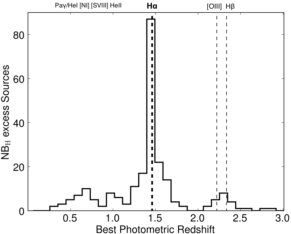
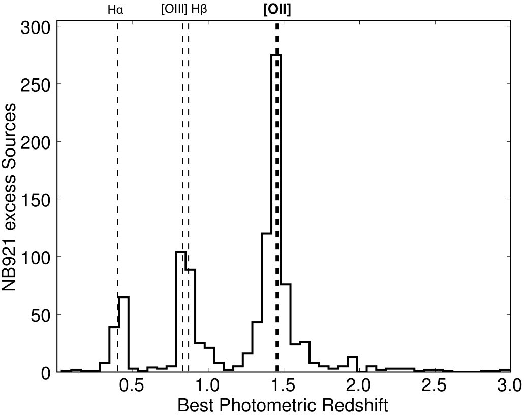
There are many possible emission-lines which can be detected individually by the NB_H and the NB921 filters. For $z<1$ galaxies, the NB_H filter is sensitive to lines such as Pa$\beta$ at $z=0.26$ or Pa$\gamma$ and HeI at $z=0.49$ or HeII at $z=0.96$, while at $z>1$ the (main) possible emission lines are H$\alpha$ at $z\sim 1.47$, [Oiii]/H$\beta$ at $z\sim 2.25$ and [Oii] at $z=3.34$, among others. The NB921 filter is mostly sensitive to H$\alpha$ at $z\sim 0.4$, [Oiii]/H$\beta$ at $z\sim 0.83$, [Oii] at $z\sim 1.47$ and Ly$\alpha$ at $z\sim 6.6$. H$\alpha$–[Oii] line emitters at $z=1.47$ can be selected with a significant narrow-band excess in both bands, and thus simultaneous excess sources provide an extremely robust means of selecting a $z=1.47$ sample. This is explained in §3.4. First, in order to select [Oii] emitters below the H$\alpha$ flux limit (see Figure 2), to assess the robustness and contamination of different selections, to investigate the range of different emitters, and to allow the selection in sky areas where coverage is not available in both filters, alternative approaches are considered.

Figure 5: A comparison between the best photometric redshifts in the UDS field and the robust spectroscopic redshift for such sources in UDS with spectroscopic redshift. NB_H excess sources with spectroscopic redshifts are all identified with a known emission line falling into the NB_H filter. It is noteworthy that the limited (and very biased towards the strongest line emitters and AGN) spectroscopic sample reveals that some confirmed H$\alpha$ emitters have photo-zs which place them at a higher and lower redshift – the use of NB921 data is able to identify these emitters which the photo-zs could miss. Vertical lines indicate the redshifts of the main emission lines detected by the NB_H filter, specifically [Ni] at $z=0.545$, [Sviii] 9914 at $z=0.625$, [Oii] 7625 at $z=1.125$, H$\alpha$ at $z=1.47$, [Oiii] 5007 at $z=2.23$ and H$\beta$ at $z=2.33$.

3.3.1 Photometric redshift analysis

Multi-wavelength data can be used to effectively distinguish between line-emitters at different redshifts (different emission lines) and separately obtain H$\alpha$ and [Oii] selected samples of galaxies at $z=1.47$ from the NB_H and NB921 data-sets. Out of 5505 NB921 potential emitters (excluding stars) within the UKIDSS UDS area, 2715 ($\approx 50$ %) have a $>3$ $\sigma$ detection in the near-IR UKIDSS data ($K~{}\lower 2.15277pt\hbox{$\buildrel<\over{\sim}$}~{}25$ AB), while all NB_H emitters are detected in $K$. Robust photometric redshifts are only available over a matched $0.64\deg^{2}$ area, mostly due to the overlap with the Subaru data and the deep Spitzer coverage (SpUDS, PI J. Dunlop), and for sources with $K<23$ (M. Cirasuolo et al., in prep.). Photo-zs are derived using a range of photometry (UBVRizJHK , together with IRAC 3.6 and 4.5 bands) and are available for 257 NB_H potential line emitters and 1021 NB921 excess sources.

Figure 6: $Top$: The $i-$K vs. B$-R$ (AB) colour-colour distribution of NB921 emitters, clearly separating the 3 types of emitters that make the bulk of the sample of emitters. Simple lines for distinguishing these emitters – supported by evolution tracks (see S09) – are also shown. $Bottom$: An equivalent plot for the NB_H emitters (AB), again demonstrating that lower redshift emitters can be easily isolated from the $z=1.47$ H$\alpha$ emitters. Higher redshift emitters, however, occupy a similar region, and can not be robustly isolated with this set of colours alone. The two pivot points for the $z\sim 0.4$ and $z\sim 0.8$ separation are [0.63,0.84] and [1.71,2.77]; while the two pivot points used to separate $z\sim 0.8$ from $z\sim 1.5$ are [0.26,0.89] and [1.17,3.39].

Figure 4 shows the photometric redshift distribution for the selected narrow-band emitters in NB_H (left panel) and NB921 (right panel) with available photometric redshifts in UDS, demonstrating the common peak at $z\sim 1.4-1.5$, associated with the H$\alpha$/[Oii] lines being detected in each narrow-band filter. In addition to this, the other peaks are easily identified as H$\alpha$ at $z=0.4$ and [Oiii]/H$\beta$ at $z=0.83$ for the NB921 emitters.

3.3.2 Spectroscopic redshift analysis

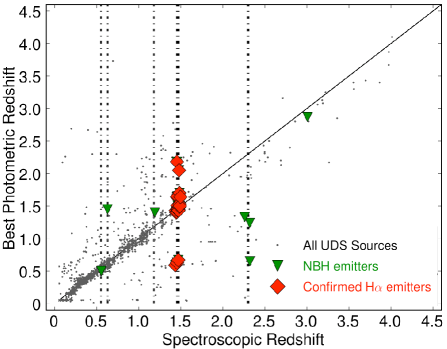
Although an extensive spectroscopic sample is not yet available in the UKIDSS-UDS field (O. Almaini et al. in prep.; H. Pearce et al. in prep.), matching the samples of emitters with all the spectroscopic redshifts published in the literature in this field (Yamada et al., 2005; Simpson et al., 2006; Geach et al., 2008; van Breukelen et al., 2007; Ouchi et al., 2008; Smail et al., 2008; Ono et al., 2010) allows the spectroscopic confirmation of 17 H$\alpha$ emitters at $z=1.455-1.48$ (over the full $0.78\deg^{2}$ area), two [Oiii] 5007 emitters at $z=2.23$, an H$\beta$ emitter at $z=2.33$, and three lower redshift emitters ([Ni] at $z=0.545$, [Sviii] 9914 at $z=0.625$ and [Oii] 7625 at $z=1.125$), for the NB_H data (see Figure 5). Furthermore, follow-up spectroscopy with SINFONI on the VLT of 6 H$\alpha$ candidates has resulted in confirming all those sources, with spectroscopic redshifts $1.45-1.47$ (A. M. Swinbank et al. in prep.), and observations with FMOS on Subaru have confirmed a further 8 H$\alpha$ emitters (E. Curtis-Lake et al., in prep.), resulting in a total of 31 spectroscopically confirmed $z\sim 1.47$ H$\alpha$ emitters.

For NB921 emitters, the limited spectroscopy confirms nine $z=0.4$ H$\alpha$ emitters, 12 $z=0.83$ [Oiii] 5007 emitters, a $z=1.1$ H$\gamma$ emitter, ten 4000Å breaks (in which the NB921 filter probed light just to the red of the break, while the $z^{\prime}$ band is dominated by emission blueward of the break, resulting in an excess in NB921), eight [Oii] emitters at $z=1.47$, nine $z=2.31$ MgII emitters (AGN) and a $z=3.87$ CIII] emitter, among others.

Figure 7: The $z-$K vs. i$-z$ (AB) colour-colour distribution of NB_H emitters, demonstrating a method to distinguish between the population of $z\sim 1.47$ H$\alpha$ emitters, which dominate the sample, and higher redshift emitters such as [Oiii] and H$\beta$ emitters at $z\sim 2.2$. The dashed line presents the simple separation used (in combination with the removal of lower redshift emitters using the criteria in Figure 6) for sources with no photometric redshifts. The colour separation is similar to the B$z$K selection, but by using the $i-z$ colour it better picks up the 4000Å break for $z=1.47$ galaxies, thus separating them better from $z\sim 2$ galaxies than using $B-z$. The two pivot points for the $z\sim 2.2$ and $z\sim 1.47$ separation are [0.09,1.50] and [0.49,3.96].

3.3.3 Colour-colour separation of emitters

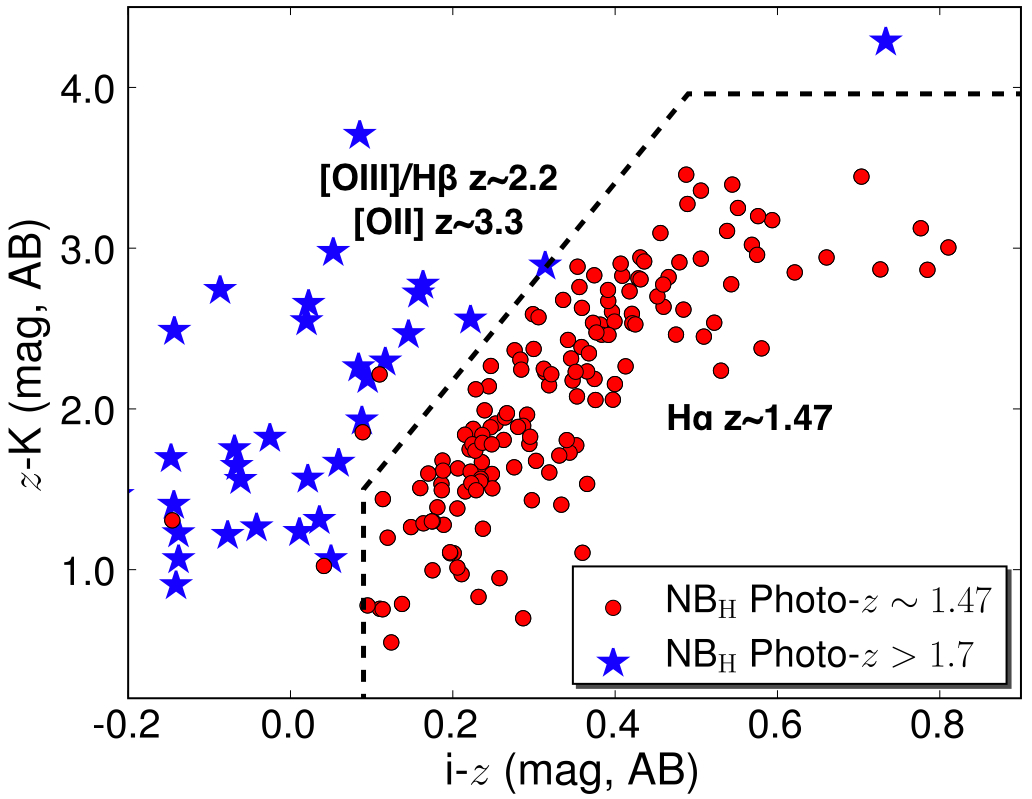
Colour-colour diagnoses can be valuable tools to explore the extremely deep broad-band photometry available, particularly for sources with no photometric redshift information (either because they are faint in the $K$-band, or because they are found outside the matched Subaru-Spitzer area). In S09, the $BRiK$ colour-colour diagram ($B-R$ vs. $i-K$) is shown to isolate $z\sim 0.8$ emitters from lower and higher redshift emitters. As Figure 6 shows, the same colour-colour separation is also suited to separate $z\sim 1.5$ emitters from lower redshift emitters. Such colour-colour space is found to be particularly suited to distinguish between the bulk of the NB921 emitters, as Figure 6 shows, clearly isolating H$\alpha$, [Oiii]/H$\beta$ and [Oii] emitters. Based on the spectroscopic confirmations and the reliable photometric redshifts, empirical colour-colour selection criteria are defined (see Figure 6) to distinguish between emitters. The same separation line produces relatively clean samples of $z>1.3$ emitters for the NB_H sample. However, for this filter the H$\alpha$ emitters at $z\sim 1.5$ and the [Oiii]/H$\beta$ emitters at $z\sim 2-3$ have similar $BRiK$ colour-colour distributions, and a new set of colours needs to be explored to separate $z\sim 1.5$ and $z>2$ emitters, after using the $BRiK$ technique to remove low-z emitters. As Figure 7 shows, $i-z$ vs. $z-K$ colours provide a good separation between $z\sim 1.5$ and $z>2$ emitters (the selection is similar to the widely used $B$$z$$K$ method, but can separate $z\sim 1.5$ galaxies from those at $z\sim 2$ and higher much more effectively), defining a colour-colour sub-space where H$\alpha$ emitters at $z=1.47$ should be found.

These results demonstrate that a relatively good selection of $z\sim 1.5$ emitters can be obtained using just 5-band ($B$$R$$i$$z^{\prime}$$K$) photometry. The $BRiK$ selection can be used to remove low-z emitters, and a further $i$$z$$K$ analysis is capable of removing higher redshift emitters (although there’s little contamination of the latter in the NB921 sample).

Figure 8: The photometric redshift distribution of simultaneous NB_H & NB921 narrow-band emitters when compared to all NB_H emitters within the NB921 imaging area. By matching both samples, it is possible to define a robust sample of H$\alpha$&[Oii] emitters without the need for colour or photometric redshift selection. Note that emitters with $K<23$ AB are not found in the photo-z catalogue, and therefore not shown in the figure.

3.4 The dual narrow-band approach at $z=1.47$

As Figure 1 demonstrates, the two narrow-band filter profiles are extremely well matched in redshift when considering the detection of the H$\alpha$ and [Oii] emission lines (although the NB921 filter probes a slightly wider range in redshift). The match can be fully explored to select robust H$\alpha$ emitters at $z=1.47$, as these should be detected as [Oii] emitters in NB921 (because of the depth of those data). Within the matched NB_H-NB921 area (out of a sample of 297 NB_H emitters), a sample of 178 dual-emitter sources is recovered. Figure 8 shows the photometric redshift distribution of the double emitters, compared with the distribution of all NB_H emitters with photo-zs (for roughly the same area). The results clearly suggest that the dual-emitter candidate criteria is able to recover essentially the entire population of $z=1.47$ H$\alpha$ emitters. Moreover, the dual-emitter selection also recovers some sources with photometric redshifts which are significantly higher (3 sources) and lower (14 sources) than $z=1.47$ (accounting for the 1 $\sigma$ error in the photo-$z$s) and that would have been missed by a simple photo-$z$ selection. There are spectroscopic redshifts available for 7 out of the 14 lower-photo-$z$ sources, and they all confirm those sources to be at $z=1.45-1.48$, indicating that their selection by the dual-emitter technique is very reliable.

The sources for which the photo-$z$ fails have high H$\alpha$ fluxes, and/or are very blue. It is therefore likely that the photo-$z$s fail for these sources because they do not present identifiable breaks (pushing photo-$z$s to a lower redshift solution), and/or because they present strong enough H$\alpha$ lines to contaminate the photometry.

3.4.1 Searching for low [Oii] EWs H$\alpha$ emitters

Figure 9 shows the distribution of [Oii]/H$\alpha$ line ratios for the emitters selected in both narrow-band filters. In order to ensure maximum completeness at the faintest [Oii] fluxes, and minimise any possible biases, a search for extra H$\alpha$ emitters with significant ($\Sigma>3$) NB921 colour-excess but low [Oii] EWs  (i.e. waiving the 25Å EW requirement), is conducted. This yields 12 additional sources above the NB921 flux limit. All of these additional sources present colours and photometric redshifts consistent with being genuine $z\sim 1.47$ sources and probe down to the lowest [Oii]/H$\alpha$ line fractions (see Figure 9); their colours are consistent with being sources affected by higher dust extinction. These 12 sources are added to the robust double-emitter sample.

Table 2: A summary of the number of sources within the different samples, including detections, candidate emitters, those within the matched area, those for which the full set of colours are available, sources with available photometric redshifts, and those selected as $z=1.47$ emitters.

Sample	NBH	NB921
NB Detections ($>3$ $\sigma$, full area)	23394	347341
Candidate emitters (full area)	439	8865
After visual+star rejection (full area)	411	8747
Matched area NBH+NB921 (0.67 sq deg)	297	5505
Selection colours available (0.67 sq deg)	297	2715
Photometric redshifts available	257	1021
Selected $z=1.47$ emitters (0.67 sq deg)	190 (H$\alpha$)	1379 ($[\rm OII]$)

3.4.2 The completeness of the H$\alpha$-[Oii] double selection

The completeness limit on the [Oii]/H$\alpha$ flux ratio (see Figure 9) indicates that the deep NB921 flux limit guarantees a very high completeness of the dual-emitter sample, and suggests that the small number of sources that photo-zs indicate as being at $z\sim 1.47$, but which are not NB921 excess sources, are actually at other redshifts. To test this further, the photometric redshift and colour-colour selections are applied in the same matched sky area. These identify 32 H$\alpha$ candidate sources which are not selected by the dual-emitter approach. Four of these sources have spectroscopic redshifts available, and all four of these are indeed spectroscopically confirmed to lie at different redshifts (cf. Figure 5). Of the remaining 28, 18 sources have significantly negative excesses in NB921, and the remaining 10 have $<3\,\Sigma$ excesses, which would correspond to a range of NB921 line fluxes from $\sim 0.1-1\times 10^{-18}$ erg s^-1 cm^-2. If real, these line fluxes would imply very low [Oii]/H$\alpha$ flux ratios, indicating that the sources must be highly extinguished (A${}_{\rm H\alpha}\sim 2-4$ mag); however, their UV and optical colours appear inconsistent with such high extinction (see §5.5). Thus, these sources are likely to be a mixture of other line emitters of weaker emission lines close to H$\alpha$ (e.g. [Nii], [Sii]), which the photometric redshifts are not sufficiently accurate to distinguish (see Sobral et al. 2009a).

3.5 Selecting robust H$\alpha$ and [Oii] ${\bf z=1.47}$ emitters

3.5.1 H$\alpha$ emitters at $z=1.47$

§ 3.4 shows that with the flux limits of this study, the NB_H-NB921 is clearly a clean and highly complete means of selecting $z=1.47$ H$\alpha$ emitters. The sample of robust H$\alpha$ emitters at $z=1.47$ is therefore derived solely by using the dual-emitter selection, within the matched area. This results in the selection of very robust 190 H$\alpha$-[Oii] sources at $z=1.47$.

Figure 9: The distribution of the [Oii]/H$\alpha$ line ratios for the robust sample of 190 simultaneous H$\alpha$-[Oii] line emitters at $z=1.47$ (the shaded region represents the 12 sources with the low [Oii] EWs). The vertical dashed line represents the lowest line ratio that the combined survey is able to probe at the lowest H$\alpha$ fluxes; this shows that the [Oii] survey is deep enough to recover essentially all H$\alpha$ emitters and that the line flux distribution is not a result of a bias caused by insufficient sensitivity at the lowest line flux ratios.

3.5.2 [Oii] emitters at $z=1.47$

In order to select [Oii] emitters, in addition to the dual-emitter selection at bright fluxes, both photo-zs and(or) colours are used. In particular, the $z=1.47$ [Oii] candidates are defined to be narrow-band excess sources with $z_{min}<1.47<z_{max}$ (where $z_{min}$ and $z_{max}$ are the 3-$\sigma$ redshift limits of the principle peak in the photometric redshift probability distribution – photo-zs of emitters have a typical $\Delta z$ of $\approx 0.13$) or those that are found within the defined $BR-iK$ colour-colour space ($(B-R)<0.26$ or $(i-K)>4.92$ or $(i-K)>4.121(B-R)+1.349$; see Figure 6). Even though the contamination from higher redshift ($z>1.5$) emitters (such as MgII) is likely to be low, the colour-colour selection presented in Figure 7 is also applied ($(i-z)<0.24$ or $(z-K)>5.33$ or $(z-K)>6.15(i-z)+1.394$), to remove potential higher redshift ($z>1.5$) emitters. This results in a sample of 1379 [Oii] selected emitters down to the flux limit of the survey. However, as noted before, many faint NB921 emitters are not detected in at least one of the bands necessary for the colour-colour identification, and therefore are not included directly in the [Oii] sample. §4.3 investigates how this can bias the determination of the faint-end of the luminosity function and derives a correction to account for the sources which are missed.

4 H$\alpha$ and [Oii] Luminosity functions

4.1 Contribution from adjacent lines

While the NB921 filter can measure the [Oii] emission line (which, in fact, is a doublet) without contamination from any other nearby emission line, this is not the case for NB_H and the H$\alpha$ line. The nearby [Nii] emission lines can contribute to the NB_H emission flux, and therefore both EWs and fluxes will be a sum of [Nii] and H$\alpha$. The limited spectroscopic follow-up in the $H$ band with sinfoni (A. M. Swinbank et al. in prep.) provides good enough S/N and spectral resolution to compute individual [Nii] fractions/corrections. The data show a range of [Nii] fractions between 0.1–0.4 and, despite being a limited sample, the results are broadly consistent with Equation 3 of S09, which estimates the [Nii] contamination as a function of total rest-frame EW₀([Nii]+H$\alpha$), based on a large SDSS sample. For the analysis presented in this paper, the polynomial approximation used in S09 has been re-computed using a higher order polynomial which is able to reproduce the full SDSS relation between the average, $\log$([Nii]/H$\alpha)$, $f$, and $\log$[EW₀([Nii]+H$\alpha$)], $E$: $f=-0.924+4.802E-8.892E^{2}+6.701E^{3}-2.27E^{4}+0.279E^{5}$. This relation is used to correct all H$\alpha$ fluxes in this paper. The average correction for the $z=1.47$ sample is 0.22 (average rest-frame EW₀(H$\alpha$+[Nii]) of 130Å).

Figure 10: A study of the completeness fraction (defined as the fraction of sources with a given flux recovered by the selection against the actual number of sources with that flux) in order to address incompleteness as a function of line flux for both NB_H and NB921 samples in the SXDF-UKIDSS-UDS field. Note that both image detection and colour-magnitude selection are taken into account as these are $both$ sources of incompleteness. This confirms the flux limit computed for both bands (down to $\sim 3\,\sigma$). Note that the NB_H curve shown is used to correct the H$\alpha$ luminosity function directly for incompleteness (for each field), while the NB921-[Oii] function plotted is the one that is used when correcting the [Oii] luminosity function (obtained by including both the flux incompleteness and the selection incompleteness – see Figure 11 and Section 4.3).

4.2 Individual line completeness

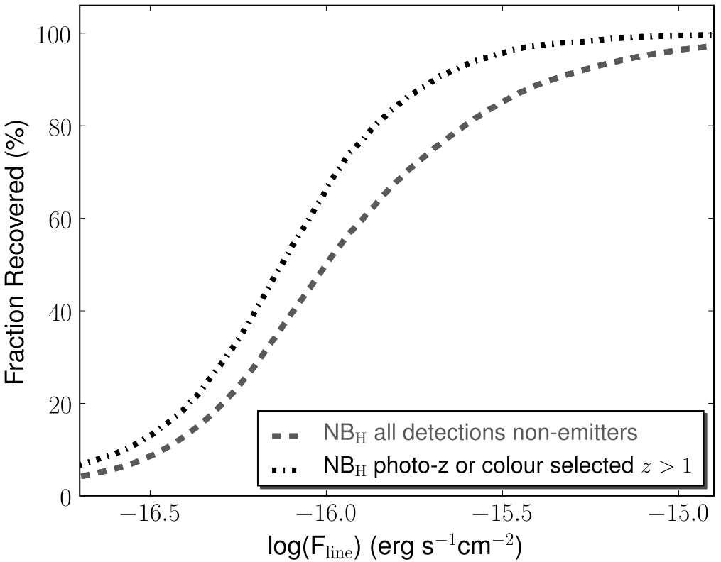
It is fundamental to understand how complete the samples are as a function of line flux. This is done using simulations, as described in S09. Briefly, the simulations consider two major components driving the incompleteness fraction: the detection completeness (which depends on the actual imaging depth and the apertures used) and the incompleteness resulting from the selection (both EW and colour significance). The first component is studied individually per frame, by adding a set of fake galaxies with a given input magnitude to each frame and obtaining both the recovery fraction and the recovered magnitude. The second component is studied by using sources which have not been selected as emitters, and adding an emission line with a given flux to all those in order to study the fraction recovered. In an improvement to S09, sources classed as stars and those occupying the $z<1$ region of the $BRiK$ diagram are not used in this simulation – this results in a set of galaxies with an input magnitude distribution which is very well-matched to the $z=1.47$ population, providing a more realistic sample to study the line completeness of the survey for $z=1.47$ H$\alpha$ emitters (see Appendix A, which quantifies the difference of using this method).

For each recovered source, a detection completeness is associated, based on its new magnitude. The results (survey average) can be found in Figure 10, but it should be noted that because of the differences in depth, simulations are conducted for each individual frame, and the appropriate completeness corrections applied accordingly when computing the luminosity function.

A similar procedure is followed for the NB921 data (average results are also shown in Figure 10); corrections are also derived and used individually for each field, although the differences in depth are not as significant as for the NB_H data. Similarly to the NB_H analysis, non-emitter sources which are classed as stars and low redshift ($z<1$) are rejected when studying how the completeness of the survey varies with line flux in order to better estimate how complete the survey is specifically for $z=1.47$ line emitters.

For any completeness correction applied, an uncertainty of 20% of the size of the correction is added in quadrature to the other uncertainties to account for possible inaccuracies in the simulations.

Figure 11: Fraction of [Oii] and non-[Oii] NB921 emitters (amongst those with $K$ detections, allowing for a colour-colour separation) as a function of emission line flux. A significant number of potential line emitters are not in the final [Oii] colour-selected sample as they are not detected in the K band imaging; the fraction of all emitters with a $K$ detection is also shown.

4.3 [Oii] selection completeness

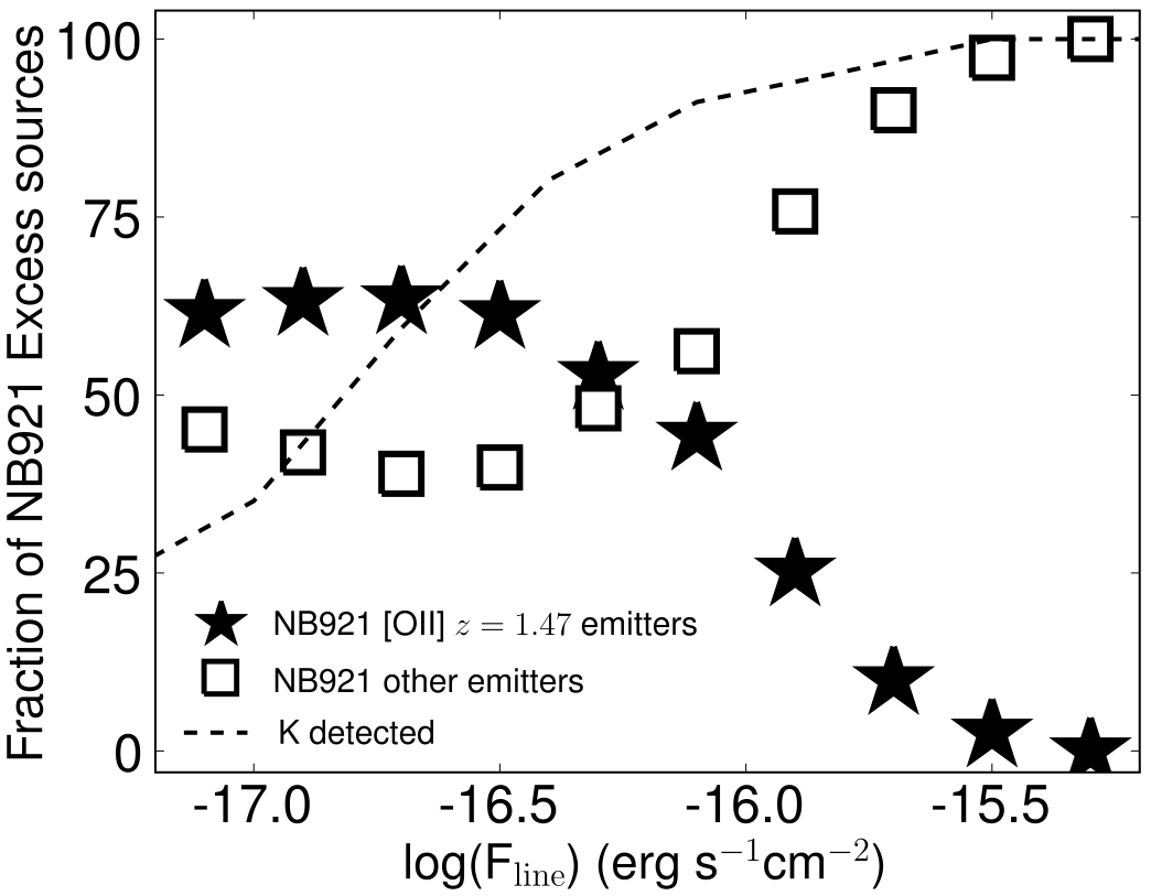
A significant fraction of NB921-selected emitters do not have photometric redshifts (79%), and half of the sample is undetected in $K$ above the $3\sigma$ limit. Therefore, these cannot be robustly classified, and they are not included in the [Oii] sample, even though at least some of them may well be genuine [Oii] emitters at $z=1.47$. This can cause a potentially significant incompleteness in the [Oii] sample, resulting in an underestimation of the luminosity function. In order to investigate this source of incompleteness and its effect in the determination of the luminosity function, the fraction of emitters with $K$ detections (which generally sets the limit for colour-colour selection, as the other bands used are significantly deeper - though even in the optical bands typically 33% of the sources are undetected) is studied as a function of line flux. As Figure 11 shows, the fraction of NB921 excess sources with $K$ detections falls as a function of decreasing line fluxes, suggesting that the incompleteness is higher at the lowest fluxes. This can have implications for determinations of the faint end slope of the luminosity function.

Figure 11 also shows that, for the classifiable sources, the fraction of [Oii] emitters rises with decreasing flux at the highest fluxes, and then seems to remain relatively flat at $\sim 60$% down to the lowest fluxes. Assuming that this same distribution is true for the unclassified sources (which is likely, since the [Oii] fraction also remains roughly constant with $K$–band magnitude for the faintest $K$ magnitudes probed), it is possible to estimate a correction at a given flux that is given by the ratio of the classifiable sources to all sources at that flux. This is equivalent to including unclassified emitters in the luminosity function calculation with a weight that is given by the fraction of [Oii] emitters at that flux (see Figure 10). An uncertainty corresponding to 20% of this correction is added in quadrature to the other uncertainties.

4.4 Volume: H$\alpha$ and [Oii] surveys

Assuming the top-hat (TH) model for the NB_H filter (FWHM of 211.1 Å, with $\lambda^{TH}_{min}=1.606\,\mu$m and $\lambda^{TH}_{max}=1.627\,\mu$m), the H$\alpha$ survey probes a (co-moving) volume of $2.667\times 10^{5}$ Mpc³. When matched to the NB921 coverage, this is reduced to $2.2872\times 10^{5}$ Mpc³ due to the reduction in area – the matched FWHM is the same. While this is the total volume probed for the common flux limit over the entire coverage, each pointing reaches a slightly different flux limit, and therefore at the faintest fluxes the volume is smaller (as only one pointing is able to probe those). This is taken into account when determining the luminosity function: only areas with a flux limit above the flux (luminosity) bin being calculated are actually taken into account. In practice, this results in only using $\sim$ one quarter of the total area for the faintest bin (with this being derived from the deeper WFCAM pointing).

Assuming a top-hat model for the NB921 filter, (FHWM of 132 Å, with $\lambda^{TH}_{min}=0.9130\,\mu$m and $\lambda^{TH}_{max}=0.9262\,\mu$m), the [Oii] survey probes a volume (over 0.67 deg²) of $2.5102\times 10^{5}$ Mpc³ when assuming a single line at 3727Å, and a volume of $2.6363\times 10^{5}$ Mpc³ using the fact that the [Oii] line is actually a doublet; 3726.1Å and 3728.8Å. For simplicity, because the change in volume is less than 5 per cent (and therefore much less than the errors), and for consistency with other authors (allowing a better comparison), the volume used assumes a single line.

4.5 Filter Profiles: volume and line ratio biases

Neither NB_H or NB921 filter profiles are perfect top-hats (see Figure 1). In order to evaluate the effect of this bias on estimating the volume (luminous emitters will be detectable over larger volumes – although, if seen in the filter wings, they will be detected as fainter emitters), a series of simulations is done. Briefly, a top-hat volume selection is used to compute a first-pass (input) luminosity function and derive the best Schechter Function fit. The fit is used to generate a population of simulated H$\alpha$ emitters (assuming they are distributed uniformly across $1.40<z<1.52$); these are then folded through the true filter profile, from which a recovered luminosity function is determined. Studying the difference between the input and recovered luminosity functions shows that the number of bright emitters is underestimated, while faint emitters are slightly overestimated (c.f. S09 for details). This allows correction factors to be estimated – these are then used to obtain the corrected luminosity function.

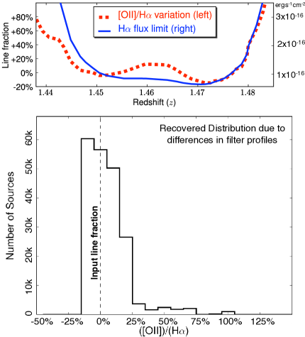
Figure 1 also shows how the NB_H and NB921 filters are very well matched, although the [Oii] coverage is slightly wider than the H$\alpha$ coverage. In order to evaluate how this might affect the results on line ratios, a series of simulations is done. Simulated [Oii]+H$\alpha$ emitters are distributed uniformly in a volume defined by $1.40<z<1.52$, which contains the entire transmission regions of both profiles. Emitters are given a wide range of H$\alpha$ fluxes based on the observed H$\alpha$ luminosity function, and [Oii] fluxes corresponding to [Oii]/H$\alpha$ line ratios between 0 and 2.0. The real filter profiles are then used to recover, for each emitter, both the [Oii] and H$\alpha$ fluxes, and therefore allow the study of both the recovered line fluxes and the recovered line ratios. Based on these results – presented in Figure 12 – the line ratios should be accurate within $\sim 20$%.

Figure 12: $Top$: the variation of the measured [Oii]/H$\alpha$ line ratio as a function of galaxy redshift due to the small differences in the transmission function of both filter profiles. Note that the flux limit (in units of erg s^-1 cm^-2) also varies very significantly as a function of redshift, and thus line ratios are likely to be correct to within less than 20% for the large bulk of the sample. $Bottom$: by using the H$\alpha$ luminosity function to produce a population of galaxies distributed over a wider redshift range than the filter profile, it is possible to use both NB_H and NB921 filter profiles to study in a simple way the distribution of the ratio between the recovered and input line fractions. The results recover the input line fraction with 17% standard deviation and with less than 1% recovered with a line fraction increased by more than +50%.

4.6 Extinction Correction

The H$\alpha$ emission line is not immune to dust extinction, although it is considerably less affected than the [Oii] emission line. Measuring the extinction for each source can in principle be done by several methods, ranging from spectroscopic analysis of Balmer decrements to a comparison between H$\alpha$ and far-infrared determined SFRs, but such data are currently not available.

In this Section, the analysis of the H$\alpha$ luminosity function is done assuming A${}_{\rm H\alpha}=1$ mag of extinction at H$\alpha$, as this allows an easy comparison with the bulk of other studies which have used the same approach. A few studies have used a H$\alpha$ dependent extinction correction – either derived from Garn et al. (2010), or from Hopkins et al. (2001). However, §5 suggests that at least the overall normalization of such relation at $z\sim 1.5$ is significantly lower (dust extinction is not as high as predicted for the very high luminosities probed) and therefore over-predicts dust-extinction corrections by $\sim 0.5-0.7$ mag (overcorrecting luminosities by $0.2-0.3$ in dex). Finally, the [Oii] luminosity function is presented without any correction for extinction, in order to directly compare it with the bulk of other studies. Detailed extinction corrections and a discussion regarding those are presented in Section 5.

4.7 H$\alpha$ Luminosity Function at $\bf z=1.47$ and Evolution

By taking all H$\alpha$ selected emitters, the luminosity function is computed. As previously described, it is firstly assumed that the NB_H filter is a perfect top-hat, but the method of S09 is applied to correct for the real profile (see Section 4.5). Candidate H$\alpha$ emitters are assumed to be all at $z=1.47$ (as far as luminosity distance is concerned). Results can be found in Figure 13. Errors are Poissonian, with a further 20% of completeness corrections added in quadrature. The luminosity function is fitted with a Schechter function defined by three parameters $\alpha$, $\phi^{*}$ and $L^{*}$:

Figure 13: The H$\alpha$ luminosity function evolution up to $z\sim 2.3$. The new measurement at $z=1.47$ is combined with HiZELS measurements (S09 and G08) and other narrow-band studies (Gallego et al., 1995; Ly et al., 2007; Shioya et al., 2008; Geach et al., 2008; Hayes et al., 2010; Tadaki et al., 2011). This confirms the strong L${}_{\rm H\alpha}^{*}$ evolution from $z=0$ to $z=2.23$.

$$\phi(L)\rm dL=\it\phi^{*}\left(\frac{L}{L^{*}}\right)^{\alpha}e^{-(L/L^{*})}\rm d\it\left(\frac{L}{L^{*}}\right).$$ (5)

In the $\log$ form the Schechter function is given by:

$$\phi(L)\rm dL=\ln 10\,\it\phi^{*}\left(\frac{L}{L^{*}}\right)^{\alpha}e^{-(L/L^{*})}\left(\frac{L}{L^{*}}\right)\rm d\log L.$$ (6)

A Schechter function is fitted to the H$\alpha$ luminosity function, with the best fit resulting in:

$\log L^{*}_{\rm H\alpha}=42.50\pm 0.23$ erg s^-1

$\log\phi^{*}_{\rm H\alpha}=-2.44\pm 0.33$ Mpc^-3

$\alpha_{\rm H\alpha}=-1.6\pm 0.4$

The best-fit function is also shown in Figure 13, together with the luminosity functions determined by Ly et al. (2007) – extending the work by Gallego et al. (1995) – at $z\approx 0$ and that from Shioya et al. (2008) at $z=0.24$. Also presented on Figure 13 are luminosity functions from the other HiZELS redshifts. The new luminosity function uses the revised catalogues presented in Sobral et al. (2010) and Sobral et al. (2011), and uses new completeness corrections, re-computed fluxes and the rest-frame EW dependent [NII] correction. The changes to the luminosity function are only minor. At $z=2.23$, the luminosity function has also been re-calculated by combining the results from Geach et al. (2008), with new ultra-deep measurements of the faint end by Hayes et al. (2010) – using HAWK-I on VLT – and Tadaki et al. (2011) – using MOIRCS on Subaru. Best fits for the HiZELS luminosity functions at $z=0.84$, $z=1.47$ and $z=2.23$ are presented in Table 3.

The results confirm the strong evolution from the local Universe to $z=2.23$ and provide further insight. In particular, while there is significant evolution up to $z\sim 0.8$, the H$\alpha$ luminosity functions at $z\sim 0.8$, $z\sim 1.47$ and $z\sim 2.23$ (including the ultra-deep measurement by Hayes et al., 2010) seem to agree well at the lowest luminosities probed (below $\log L_{\rm H\alpha}\sim 42.0$) in normalisation and slope – all consistent with a relatively steep value of $\alpha\sim-1.6$) – a similar $\alpha$ is found by Ly et al. (2011). In contrast, at the bright end, L${}_{\rm H\alpha}^{*}$ is clearly seen to continue to increase from $z=0.84$ to $z=1.47$ and to $z=2.23$, with $\log\,L^{*}\propto 0.6z$. This implies that the bulk of the evolution from $z=2.23$ to $z\sim 1$ is happening for the most luminous H$\alpha$ emitters (L${}_{\rm H\alpha}>10^{42}$ erg s^-1), which greatly decrease their number density as the Universe ages: the faint-end number densities seem to remain relatively unchanged.

Table 3: The luminosity function and star-formation rate density evolution at the peak of the star formation history as seen by HiZELS at $z=0.84$, $z=1.47$ and $z=2.23$; assuming 1 mag extinction at H$\alpha$. Columns present the redshift, break of the luminosity function, $L^{*}_{H\alpha}$, normalisation, $\phi^{*}_{H\alpha}$ and faint-end slope of the luminosity function, $\alpha$. The three right columns present the star formation rate density at each redshift based on integrating the luminosity function down to the given luminosity limit (in $\log$ erg s^-1). Star formation rate densities include a correction for AGN contamination of 10% at $z=0.84$ (c.f. Garn et al. 2010) and 15% at both $z=1.47$ and $z=2.23$.

Epoch	$L^{*}_{H\alpha}$	$\phi^{*}_{H\alpha}$	$\alpha_{H\alpha}$	$\rho_{SFRH\alpha}$ 42	$\rho_{SFRH\alpha}$ 40	$\rho_{SFRH\alpha}$ All
(z)	erg s-1	Mpc-3		M⊙ yr-1 Mpc-3	M⊙ yr-1 Mpc-3	M⊙ yr-1 Mpc-3
$z=0.84\pm 0.02$	$42.25\pm 0.16$	$-2.36\pm 0.29$	$-1.66\pm 0.34$	$0.03\pm 0.01$	$0.12\pm 0.04$	$0.13\pm 0.06$
$z=1.47\pm 0.02$	$42.50\pm 0.23$	$-2.44\pm 0.33$	$-1.6\pm 0.4$	$0.06\pm 0.02$	$0.15\pm 0.06$	$0.16\pm 0.05$
$z=2.23\pm 0.02$	$43.07\pm 0.24$	$-2.93\pm 0.41$	$-1.60\pm 0.21$	$0.12\pm 0.06$	$0.20\pm 0.09$	$0.22\pm 0.10$

4.8 The [Oii] Luminosity function at $\bf z=1.47$ and Evolution

The [Oii] luminosity function at $z=1.47$ (not corrected for dust extinction) is shown in Figure 14. Note that this includes corrections for i) incompleteness in both detection and flux selection, ii) incompleteness in the redshift selection of [Oii] emitters (see Figure 10 for the combined correction) and iii) correction for the filter profile not being a perfect tophat. Errors are Poissonian and include (in quadrature) 20% of the completeness correction applied). The fully-corrected [Oii] luminosity function is found to be well-fitted by a Schechter function, with the best fit resulting in:

$\log L^{*}_{\rm[O{\sc II}]}=41.71\pm 0.09$ erg s^-1

$\log\phi^{*}_{\rm[O{\sc II}]}=-2.01\pm 0.10$ Mpc^-3

$\alpha_{\rm[O{\sc II}]}=-0.9\pm 0.2$

Figure 14: The [Oii] luminosity function derived from this study, at $z=1.47$ and a comparison with measurements at different redshifts from Gallego et al. (2002); Takahashi et al. (2007); Ly et al. (2007); Bayliss et al. (2011) and with a measurement at the same redshift (using the same narrow-band filter, but on a different field) by Ly et al. (2007). There is a clear evolution in the [Oii] luminosity function, at least up to $z\sim 2$.

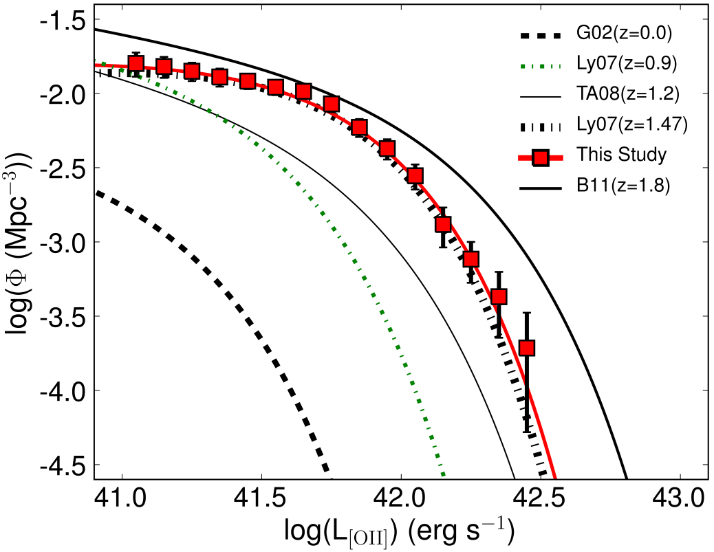
The results are compared with other studies at different redshifts (Hogg et al., 1998; Gallego et al., 2002; Takahashi et al., 2007; Ly et al., 2007; Bayliss et al., 2011) – all uncorrected for dust extinction – and shown in Figure 14. The comparison reveals a significant evolution in the [Oii] luminosity function from $z\approx 0$ to $z=1.47$. Such evolution seems to be simply described by a $\phi^{*}$ and L^∗ evolution up to $z\sim 0.9$ and a continuing L^∗ evolution from $z\sim 0.9$ up to $z\sim 2$, in line with the results for the evolution of the H$\alpha$ luminosity function. It should also be noted that there is good agreement with the Ly et al. (2007) luminosity function at the same redshift derived from a smaller area, but at a similar depth.

The correction for redshift/emitter selection is found to be particularly important at faint fluxes, setting the slope of the faint-end of the luminosity function (although it has little effect on the values of $L^{*}$ and $\phi^{*}$). If no correction for unclassified sources is applied, the best-fit Schechter function yields $\alpha\approx-0.2$ (compared to the corrected best-fit of $\alpha\approx-0.9$). In the extreme case where all the non-selectable emitters are assumed to be [Oii], it would yield $\alpha\approx-1.8$. This makes it clear that the crucial data that one needs in order to improve the determination of the faint-end slope is not new, deeper NB921 data, but rather significantly deeper $B$, $i$, $z$ and $K$ data, which will enable to completely distinguish between different line emitters at faint fluxes (or at least provide a more robust correction by classifying a much higher fraction of emitters).

Figure 15: The star formation rate density and its evolution with redshift up to $z\sim 2.3$ using H$\alpha$ only, but also including the [Oii] measurement presented in this paper (assuming 1 magnitude of extinction at H$\alpha$) and compared to estimates at different redshifts from the literature (e.g. Hopkins, 2004; Ly et al., 2011, and references herein). Darker circles represent the results from H$\alpha$ studies which are also shown in Figure 13. This confirms a strong evolution in the star formation rate density over the last $\sim 10$ Gyrs, with a flattening or slow decline over $1<z<2$ and a sharp decrease from $z\sim 1$ to $z\sim 0$.

4.9 Evolution of the H$\alpha$ and [Oii] Luminosity Functions

Robust measurements of the evolution of both the H$\alpha$ and [Oii] luminosity functions up to $z\sim 2$ have been presented. The results reveal that there is a strong, and consistent, evolution of both luminosity functions. Moreover, while the evolution up to $z\sim 1$ can be described as both an increase of the typical luminosity (L^∗) and an increase of the overall normalization of the luminosity functions ($\phi^{*}$), at $z>1$ the bulk of the evolution can be simply described as a continuous increase in L^∗ given by $\log\,L^{*}\propto 0.6z$. The current results also show that the faint-end slope (and the number density of the faintest star-forming galaxies probed) seems to remain relatively unchanged during the peak of the star formation history ($z\sim 1-2$). Of course, the latter does not imply, at all, that the faint population is not evolving. Furthermore, particularly beyond $z\sim 1$, AGN contamination at the highest luminosities could still be polluting the view of the evolution of the star-forming population.

4.10 The star formation rate density at $\bf z=1.47$

The best-fit Schechter function fit to the H$\alpha$ luminosity function can be used to estimate the star formation rate density at $z=1.47$. The standard calibration of Kennicutt (1998) is used to convert the extinction-corrected H$\alpha$ luminosity to a star formation rate:

$${\rm SFR}({\rm M}_{\odot}{\rm yr^{-1}})=7.9\times 10^{-42}~{}{\rm L}_{\rm H\alpha}~{}({\rm erg\,s}^{-1}),$$ (7)

which assumes continuous star formation, Case B recombination at $T_{e}=10^{4}$ K and a Salpeter initial mass function ranging from 0.1–100 M_⊙. A constant 1 magnitude of extinction at H$\alpha$ is assumed for the analysis, as this is a commonly adopted approach which is a good approximation at least for the local Universe. §5 will investigate this further based on the analysis of emission-line ratios, revealing that A${}_{\rm H\alpha}\sim 1$ mag for the sample presented in this paper. A 15% AGN contamination is also assumed (Garn et al. 2010 found AGN $\sim 10$% contamination at $z=0.84$, but the contamination is likely to be higher at higher redshift and the slightly higher flux limit of this sample). Down to the survey limit (after extinction correction, L${}_{\rm H\alpha}=10^{42}$erg s^-1), one finds $\rho_{\rm SFR}=0.07\pm 0.01$ M_⊙ yr^-1 Mpc^-3; an integration extrapolating to zero luminosity yields $\rho_{\rm SFR}=0.16\pm 0.05$ M_⊙ yr^-1 Mpc^-3. Furthermore, by using the standard Kennicutt (1998) calibration of [Oii] as a star formation tracer (calibrated using H$\alpha$):

$${\rm SFR}({\rm M}_{\odot}{\rm year^{-1}})=1.4\times 10^{-41}~{}{\rm L}_{\rm[OII]}~{}({\rm ergs\,s}^{-1}),$$ (8)

it is also possible to derive an [Oii] estimate of the star formation rate density at the same redshift, by using the complete integral of the [Oii] luminosity function determined at $z=1.47$, and assuming the same 1 magnitude of extinction at H$\alpha$. This yields $\rho_{\rm SFR}=0.17\pm 0.04$ M_⊙ yr^-1 Mpc^-3, in very good agreement with the measurement obtained from H$\alpha$.

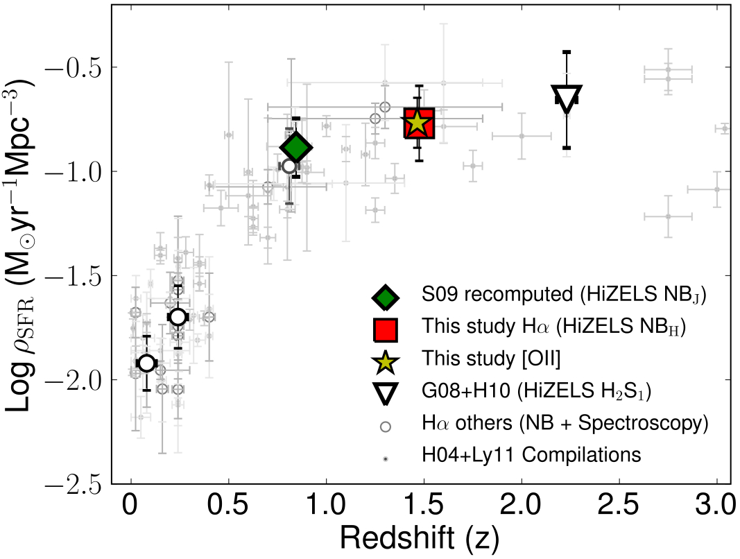
By taking advantage of the other HiZELS measurements, and other H$\alpha$ based measurements, it is possible to construct a full and consistent view of the H$\alpha$-based star formation history of the Universe. This is done by integrating all derived luminosity functions down to a common luminosity limit of L_Hα=10^41.5erg s^-1. The results are presented in Figure 15, revealing a strong rise in the star formation activity of the Universe up to $z\sim 1$ and a flattening or a small continuous increase beyond that out to $z>2$.

5 The matched H$\alpha$-[Oii] view

This section presents a detailed comparison of [Oii] and H$\alpha$ luminosities and line flux ratios (observed and corrected for dust-extinction) as a function of galaxy colour, mass and luminosity for the sample of matched H$\alpha$ and [Oii] emitters at $z=1.47$. These are compared with equivalent results for a similarly-selected sample at $z\sim 0.1$ drawn from the SDSS.

5.1 A SDSS sample at $\bf z\sim 0.1$

In order to compare the $z=1.47$ H$\alpha$+[Oii] sample with a large local sample and provide a further insight into any important correlations between line fractions and dust-extinction, mass and colour, an SDSS sample was used. Data were extracted from the MPA SDSS derived data products catalogues. The sample was defined to emulate a narrow-band slice at $0.07<z<0.1$ (chosen to be distant enough so that the fibers capture the majority of the light – typically $\sim 3-4$ kpc diameter, but not too far out in redshift to guarantee that the sensitivity is still very high and the measurements are accurate). The sample was selected by further imposing a requirement that L${}_{H\alpha}>10^{40.6}$ erg s^-1 (observed, not aperture or dust extinction corrected); this guarantees high S/N line ratios and that the vast majority of sources are detected in [Oii] as well, allowing unbiased estimates of the line ratio distribution, as well as the detection of other emission lines (Oiii], H$\beta$ and [Nii]) that can be used to distinguish between AGN and star-forming galaxies (c.f. Rola et al., 1997; Brinchmann et al., 2004). Among 17354 SDSS $z\sim 0.1$ H$\alpha$ emitters, 498 were classified as AGN, implying a $\sim 3$ per cent contamination. Potential AGN were removed from the sample. Emission line fluxes are aperture corrected following a similar procedure as in Garn & Best (2010) – i.e., by using the ratio between the fiber estimated mass and the total mass of each galaxy. For 32 galaxies where the catalogued fiber mass is higher than the catalogued total mass, an aperture correction factor of 1.0 was assigned. For those in which the fiber mass had not been determined, the average correction for the total mass of that galaxy was assigned. The median fraction of flux within the SDSS apertures is 32%. Note that the even though these aperture corrections change the total fluxes, line ratios remain unchanged. Finally, in order to provide a more direct comparison with the sample at $z=1.47$, an EW cut of 20 Å in H$\alpha$ was applied (to mimic the selection done at $z=1.47$), and galaxies with lower EWs were excluded (1701 galaxies). The final SDSS sample contains 14451 star-forming H$\alpha$ selected galaxies at $0.07<z<0.1$.

5.2 Calibrating [Oii]/H$\alpha$ line ratio as a dust extinction probe

Due to the difference in rest-frame wavelength of the [Oii] and H$\alpha$ emission lines, and both emission-lines being tracers of recent star-formation, the [Oii]/H$\alpha$ line ratio is sensitive to dust-extinction, even though metallicity can affect the line ratio as well. After correcting for dust extinction, several studies find a [Oii]/H$\alpha$ average of $\approx 1.0-1.4$ in the local Universe (c.f. Kewley et al., 2004).

The H$\alpha$/H$\beta$ line ratio (Balmer decrement) is widely used as an extinction estimator, particularly up to $z\sim 0.4$, as it is relatively easy to obtain both emission lines. As the SDSS-derived sample is able to obtain reliable fluxes for the [Oii], H$\beta$ and H$\alpha$ emission lines, it is possible to investigate (and potentially calibrate) [Oii]/H$\alpha$ as a dust-extinction indicator, using the Balmer decrement directly. As Figure 16 shows, [Oii]/H$\alpha$ is relatively well correlated with H$\alpha$/H$\beta$, indicating that it is possible to use [Oii]/H$\alpha$ to probe dust extinction within the observed scatter. For each galaxy in the SDSS-derived sample at $z\sim 0.1$, H$\alpha$/H$\beta$ line fluxes are measured and used to estimate the extinction at H$\alpha$, A_Hα, by using:

Figure 16: The variation of [Oii]/H$\alpha$ line ratios as a function of H$\alpha$/H$\beta$ ratios for SDSS (balmer decrement), showing that they correlate well, and therefore it is possible to calibrate the observed [Oii]/H$\alpha$ line ratio as a dust extinction indicator. The best polynomial fit to the data is also shown, together with the prediction from the Calzetti et al. extinction law.

$$A_{\rm H\alpha}=\frac{-2.5k_{\rm H\alpha}}{k_{\rm H\beta}-k_{\rm H\alpha}}~{}{\rm log}_{10}\left(\frac{2.86}{{\rm H\alpha}/{\rm H\beta}}\right),$$ (9)

where 2.86 is the assumed intrinsic H$\alpha$/H$\beta$ line flux ratio, appropriate for Case B recombination, temperature of $T=10^{4}$ K and an electron density of $n_{\rm e}=10^{2}$ cm^-3 (Brocklehurst, 1971). The Calzetti et al. (2000) dust attenuation law is used to calculate the values of $k_{\lambda}\equiv A_{\lambda}/E(B-V)$ at the wavelengths of the H$\alpha$ and H$\beta$ emission lines, resulting in:

$$A_{\rm H\alpha}=6.531\log_{10}\rm H\alpha/H\beta-2.981.$$ (10)

By using the Calzetti law, it is also possible to write a similar relation by using [Oii]/H$\alpha$:

$$A_{\rm H\alpha}=-2.296\log_{10}\rm[OII]/H\alpha+2.29\log_{10}(R_{0}),$$ (11)

where $R_{0}$ is the unknown intrinsic [Oii]/H$\alpha$, but the slope of the relation is fully determined. Figure 16 shows that the Calzetti law matches the global trend well, but fails to predict the fine details. The failure to match the data perfectly results from a combination of different factors. The Calzetti et al. law does not include important variations of the intrinsic [Oii]/H$\alpha$ line fraction with e.g. metallicity. The Calzetti et al. extinction law is also based on a relatively small number of local galaxies, and, most of all, it is based on continuum light, and not on emission-lines. However, it is possible to obtain a much better fit to the relation between [Oii]/H$\alpha$ ($\Psi$) and Balmer decrement with a 4th order polynomial (shown in Figure 16), and to derive an empirical relation between A_Hα directly from H$\alpha$/H$\beta$:

$$\rm A_{\rm H\alpha}=-4.30\Psi^{4}-11.30\Psi^{3}-7.39\Psi^{2}-2.94\Psi+0.31$$ (12)

with a scatter of $0.28$ mag (in A_Hα). The scatter may be driven by the range of metallicities within the sample, as galaxies will have slightly different intrinsic [Oii]/H$\alpha$ line ratios.

Figure 17: The difference between A_Hα estimated using equation 12 and directly using the Balmer decrement, as a function of a metallicity (from Equation 13). The results show that the empirical calibration derived is able to use [Oii]/H$\alpha$ line ratios as dust extinction probe without any significant bias for a relatively wide range of metallicities/abundances. A comparison with what would be obtained using the Calzetti law directly is also shown, highlighting that the polynomial fit is able to provide a calibration of [Oii]/H$\alpha$ which is less affected by metallicities. Solar metallicity corresponds to 12+$\log 10$ of 8.66; the figure presents metallicities varying from $\approx 0.2$ to $\approx 2.2$ solar metallicities. Note that while Equation 12 provides reliable results (without any significant systematics/biases) for galaxies with abundances (12+$\log 10$) from 8.2 to 8.75, it will overestimate the median A_Hα by about +0.2 mag for very sub-solar and very super-solar metallicity galaxies.

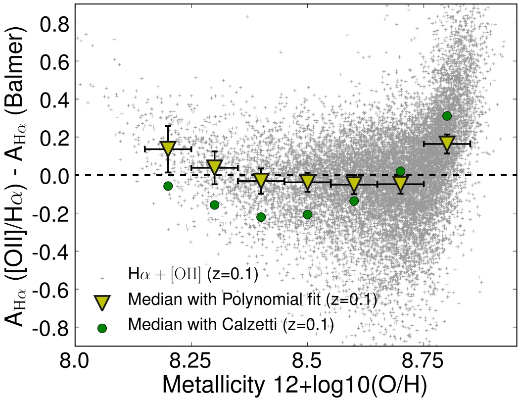
The SDSS data can be used to investigate how the offset of a galaxy from the [Oii]/H$\alpha$ vs H$\alpha$/H$\beta$ relation depends upon metallicity, and thus it is possible to measure the extent to which the [Oii]/H$\alpha$ line ratio can be used to probe extinction, without metallicity biases. Here, the O3N2 indicator (Pettini & Pagel, 2004) is used as a tracer of metallicity (the gas-phase abundance of oxygen relative to hydrogen), computed by using:

$$\rm 12+\log 10(O/H)=8.73-0.32\times\log_{10}(O3H\beta/N2H\alpha),$$ (13)

where O3H$\beta$ is the line flux ratio [Oiii]5007/H$\beta$ and N2H$\alpha$ is the line flux ratio [Nii]6584/H$\alpha$. This indicator has the main advantages of i) using emission lines which have very similar wavelengths, thus being essentially independent of dust attenuation and ii) having a unique metallicity for each line flux ratio. Figure 17 shows the difference between A_Hα computed with the empirical [Oii]/H$\alpha$ and A_Hα estimated directly from the Balmer decrement, as a function of metallicity. For comparison, the Calzetti law prediction is also shown, emphasizing that the mismatch between the latter law and the observational data is mostly due to the the effect of metallicity on the [Oii]/H$\alpha$ ratio, which is not taken into account by Calzetti, but is incorporated in the empirical calibration presented in this work. The results suggest that even if galaxies at $z=1.47$ have different metallicities from those in SDSS, no significant offset (within the scatter, $\pm 0.3$ mag) is expected when estimating A_Hα from [Oii]/H$\alpha$ for a wide range of metallicities.

For the remaining of the analysis, A_Hα is computed as in equation 12, both for the $z=1.47$ and the SDSS samples. It should be noted that the qualitative and quantitative results remain unchanged if Balmer decrements are used instead to estimate A_Hα for the SDSS galaxies, and that qualitative results also remain unchanged if the Calzetti law/best linear fit is used instead of the polynomial fit. The sample of H$\alpha$ emitters at $z=0.1$ presents A${}_{\rm H\alpha}=0.97\pm 0.42$, while the sample of H$\alpha$ emitters at $z=1.47$ presents A${}_{\rm H\alpha}=1.0\pm 0.6$.

Figure 18: A comparison between observed [Oii] and H$\alpha$ luminosities (not corrected for dust-extinction) for samples at $z\sim 0.1$ and $z\sim 1.5$. The correlation between observed luminosities seem to evolve very little in the last $\sim 9$ Gyrs, revealing a typical 1 mag of extinction at H$\alpha$ for the probed luminosities. Lines of constant extinction are also shown – note that these are not evenly spaced due to the use of the non-linear relation (Equation 12).

5.3 [Oii]-H$\alpha$ luminosity correlation at $z=1.47$ and $z\sim 0.1$

Figure 9 presents the distribution of [Oii]/H$\alpha$ line ratios for the $z=1.47$ sample. While it reveals a relatively wide range within the sample, ($\approx 0.08-1.2$), it also shows that down to the H$\alpha$ flux limit, the line ratio distribution peaks at $\approx 0.5$ (a bit above the median value, $\approx 0.45$). In the SDSS-derived sample, the line ratios show a similar range from $0.1-1$ (c.f. Hopkins et al., 2003) and the median observed line ratio is found to peak at $\approx 0.4$. Thus, even though the H$\alpha$ and [Oii] luminosities in the $z=1.47$ sample are much higher than those probed locally, the typical line ratio, if anything, is higher, indicating lower extinction.

Figure 19: The relation between dust extinction and star formation rates (uncorrected and corrected for dust extinction) based on the H$\alpha$ emission lines for both $z=1.47$ and $z=0.1$. The $top$ panel shows the relation between dust extinction at H$\alpha$ and observed H$\alpha$ SFRs. The figure also shows the Hopkins et al. (2001) relation; this consistently over-predicts the dust extinction correction of the $z=1.47$ sample by $\sim 0.5$ mag and, although it agrees better with the $z=0.1$ sample, it over-predicts the slope of the correlation. The $bottom$ panel presents the relation between A_Hα and dust extinction-corrected SFRs for both redshifts. Note that because both samples are H$\alpha$ selected, there are strong selection biases affecting the H$\alpha$ analysis (dashed lines, resulting from the approximate selection limit in the two samples, and from using A_Hα to correct SFRs for extinction), but the trends are still recovered even when accounting for such biases. The results show that even though the trends are similar at both $z=0.1$ and $z=1.47$, the normalisation is different, and the trends have evolved between $z\sim 1.5$ and $z\sim 0$.

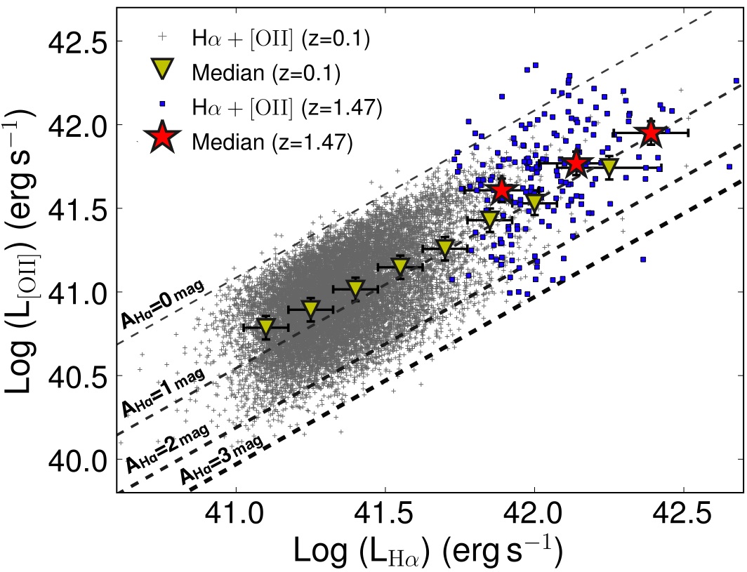
This is investigated in more detail in Figure 18, which shows how the H$\alpha$ and [Oii] luminosities (not corrected for extinction) correlate over the range of luminosities probed by SDSS at $z\sim 0.1$ and HiZELS at $z=1.47$. Lines of constant extinction (in H$\alpha$) are also shown. It is noteworthy that at a given observed H$\alpha$ luminosity, the median [Oii] luminosities are slightly higher (indicating lower median extinction) at the higher redshift. Both samples show weak trends for increasing extinction with increasing luminosity. Furthermore, it should be noted that the simple assumption that both samples present a typical constant extinction of 1 magnitude is a relatively good approximation.

Hopkins et al. (2001) find that there is a correlation between SFR and A_Hα, and so argue that it is possible to estimate (statistical) dust extinction corrections based on observed SFRs, particularly for H$\alpha$ (but also for the [Oii]-derived SFRs); their relation has been used to apply statistical corrections to the observed H$\alpha$ luminosities in many studies at low and high redshift. On the other hand, the Hopkins SFR-A_Hα relation, whilst derived with a relatively small sample in the local Universe, seems to be roughly valid at $z\sim 0.84$, as found by Garn et al. (2010) (which presents a similar analysis to Hopkins et al., i.e. comparing mid-infrared SFRs with H$\alpha$), although it slightly overestimates the amount of dust extinction of the sample. Nevertheless, it is unclear whether a similar result can be found when studying A_Hα as a function of SFRs at $z=1.47$, or if the result from Hopkins et al. (2001) can be recovered when using emission-line ratios (e.g. Balmer decrement, or the [Oii]/H$\alpha$ calibration) at $z\sim 0.1$.

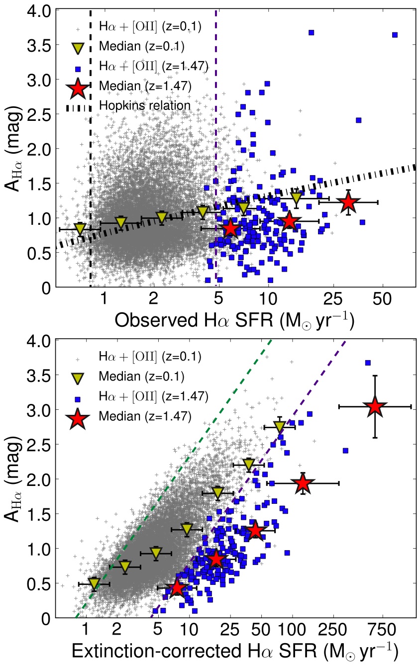
Figure 19 presents the results of investigating the dependence of dust-extinction on observed H$\alpha$ SFR for both samples. The results show a relatively weak correlation between A_Hα and observed H$\alpha$ SFRs at both $z=0.1$ and $z=1.47$; an offset in the median extinction for a given SFR between both epochs is also found.

The figure also shows the Hopkins et al. (2001) relation between A_Hα and observed SFRs, with the results showing that it consistently over-predicts the dust extinction correction of the $z=1.47$ sample by $\sim 0.5$ mag ($\sim 1.6\times$) and, although it agrees better with the $z=0.1$ sample (in the normalisation), it over-predicts the slope of the correlation. Note that A_Hα at $z=1.47$ are potentially overestimated for extremely metal-poor or metal-rich galaxies, so the offset is robust and, if anything, is underestimated. The SDSS results remain completely unchanged when using the Balmer decrement A_Hα. Therefore the use of the Hopkins et al. relation to correct observed H$\alpha$ SFRs as a function of observed SFRs/luminosity results in a clear overestimation of the dust-extinction correction at $z=1.47$; re-normalising it by $\sim 0.5$ mag is able to solve this.

Nevertheless, there seems to be a correlation between SFR and A_Hα at $z\sim 1.5$, which is more clearly revealed after correcting SFRs for dust extinction, as can be seen in Figure 19. It should however be noted that such relation is in part a result of a bias (as indicated in Figure 19), as for a given flux limit and a (wide) distribution of dust extinction corrections, one easily recovers a relation between extinction and corrected SFRs (as correcting SFR for extinction relies on A_Hα). The relation between extinction and SFR is clear at the highest H$\alpha$ luminosities where such selection biases are negligibly small. The offset between the A_Hα vs corrected-SFR relations between $z=0.1$ and $z=1.47$ is also clear at these high SFRs, and is still recovered even when a common H$\alpha$ luminosity limit is applied to both samples. These results indicate that although there does appear to be a relationship between dust extinction and SFR, this relation appears to evolve with redshift and should not be used as a reliable way of estimating statistical dust extinction corrections for samples of galaxies at different redshifts.

5.4 Mass as a dust-extinction indicator

Recently, Garn & Best (2010) performed a detailed investigation of the correlations between dust extinction (A_Hα) and several galaxy properties (e.g. metallicity, star formation rate, stellar mass) using large SDSS samples. The authors find that although A_Hα roughly correlates with many galaxy properties, stellar mass seems to be the main predictor of dust extinction in the local Universe (see also Gilbank et al., 2010, for a similar analysis). The authors derive a polynomial fit to the observed trend, which can be used to estimate dust extinction corrections for galaxies with a given stellar mass in the local Universe. Nonetheless, so far no study has been conducted in order to test whether such relation exists at high redshift and whether it evolves significantly.

5.4.1 Estimating stellar masses at $z=1.47$

In order to investigate any potential correlation between dust extinction and stellar mass at $z\sim 1.5$, stellar masses are obtained for the entire $z=1.47$ sample, following the methodology fully described in Sobral et al. (2011). Very briefly, the multi-wavelength data available for the $z=1.47$ sources are used to perform a full SED $\chi^{2}$ fit with a range of models – normalised to one solar mass – to each galaxy; the stellar-mass is the factor needed to re-scale the luminosities in all bands from the best model to match the observed data. As in Sobral et al. (2011), the SED templates are generated with the stellar population synthesis package developed by Bruzual & Charlot (2003), but the models are drawn from Bruzual (2007). SEDs are produced assuming a universal initial mass function (IMF) from Chabrier (2003) and an exponentially declining star formation history with the form $e^{-t/\tau}$, with $\tau$ in the range 0.1 Gyrs to 10 Gyrs. The SEDs were generated for a logarithmic grid of 220 ages (from 0.1 Myr to 4.3 Gyr – the maximum age at $z=1.47$). Dust extinction was applied to the templates using the Calzetti et al. (2000) law with $E(B-V)$ in the range 0 to 0.8 (in steps of 0.1). The models are generated with a logarithmic grid of 6 different metallicities, from sub-solar to super-solar metallicity. It is assumed that all H$\alpha$ emitters are at $z=1.47$ and the complete filter profiles are convolved with the generated SEDs for a direct comparison with the observed total fluxes. For all except 5 sources (1 with no $U$ band data, and 4 not detected in any IRAC band), 16 bands are used, spanning from the CFHT $U$ band in the near-ultra-violet to the 4 IRAC bands (M. Cirasuolo et al., in prep.). The appropriate corrections (c.f. Sobral et al. 2011) are applied to obtain total fluxes in each band.

Figure 20: The relation between dust extinction (A_Hα) and stellar mass for the samples at $z=0.1$ and $z=1.47$. Individual galaxies from both samples and the median are presented. The relation derived by Garn & Best (2010) is also shown, which is found to describe the relation very well for $z=0.0-1.5$ at least for low and moderate masses, indicating that stellar mass is likely a fundamental property for predicting dust-extinction corrections. The most massive star-forming galaxies (log Mass$>10.75$) may have different extinction properties at $z=0.1$ and $z=1.5$, although that may well be a result of the small number of such galaxies at $z=1.5$.

Stellar mass estimates of each individual source are found to be affected by a 1$\sigma$ error (from the multi-dimension $\chi^{2}$ distribution) of $\sim 0.30$ dex, which results from degeneracies between the star formation time-scale $\tau$, age, extinction and, to a smaller extent, metallicity. As the analysis uses a Chabrier IMF, stellar masses are directly comparable with SDSS masses (which are the ones used by Garn & Best, 2010), but note that there is a systematic offset when compared to Salpeter (see Sobral et al., 2011). It should also be noted that the $E(B-V)$ from the best fits correlate well with the A_Hα determined for each individual galaxy.

5.4.2 Mass-Extinction relation

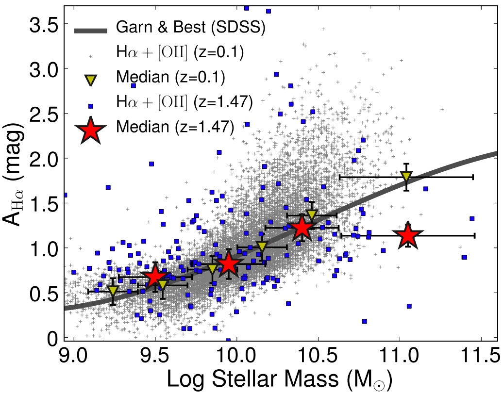
The sample of $z=1.47$ emitters presents a median stellar mass of 10^9.9 M_⊙. Figure 20 shows the observed relation between A_Hα and stellar mass, for both $z=0.1$ and $z=1.47$ samples, together with the Garn & Best (2010) relation. The results reveal that not only is there a correlation between stellar mass and dust extinction at $z=1.47$, just like the one at $z\sim 0$, but, even more importantly, that the Garn & Best (2010) relation seems to be valid at least up to $z\sim 1.5$ as a dust extinction estimator for most masses. As shown above, this is in contrast with SFR-dependent extinction corrections, which must at least be re-normalised when being applied to $z\sim 1.5$ or $z\sim 0$, and provides an important insight into what is important in determining the dust properties of galaxies. Table 4 presents the Garn & Best (2010) relation for predicting A_Hα as a function of stellar mass, which can be applied, at least within the studied range of masses, to derive statistical corrections for samples of galaxies up to $z\sim 1.5$.

Although the relation between stellar mass and A_Hα seems to hold across redshift for most masses probed, there is tentative evidence of an offset at the highest masses, in the sense that the most massive $z=1.47$ star-forming galaxies appear to be affected by significantly less dust extinction that those with comparable masses at $z=0.1$. The sample at high masses remains relatively small, however, and also since these massive star-forming galaxies are all of very low H$\alpha$ EWs (see Sobral et al. 2011), there is the possibility that selection effects are driving this result. Until this can be investigated with an improved sample, however, caution should be taken in applying the mass-extinction relation at high redshifts for masses above $\sim 10^{10.75}$ M_⊙.

5.5 Predicting A_Hα dust-extinction with colours

Stellar mass seems to be a relatively reliable (and important) non-evolving dust-extinction predictor which can therefore be applied both in the local Universe and at higher redshift ($z\sim 1.5$), at least within a range a masses. However, computing reliable stellar masses requires obtaining a significant number of observations at different wavelengths, relies on the validity of the stellar population models used to compute mass to light ratios, and it is, in general, a difficult quantity to estimate, particularly at high redshift. There is therefore the need to investigate more direct observables as a way to predict the median dust extinction of a population of galaxies that could be applied out to $z\sim 1.5$. Rest-frame optical colours are expected to correlate with dust extinction, and are therefore investigated and calibrated as dust-extinction tracers. All colours presented in this section are given in the AB system and are rest-frame colours computed using the SDSS filters.

Figure 21: The relation between dust extinction and rest-frame $u-z$ colour for the samples at $z=0.1$ (SDSS) and $z=1.47$. The data are used to derive an empirical relation which is valid for H$\alpha$ emitters both at $z=0.1$ and $z=1.47$ and predicts median dust extinction corrections (A_Hα) based on $u-z$ colours. Table 4 presents the best-fit polynomial relations based on other rest-frame colours which also correlate well with A_Hα.

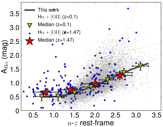
Figure 21 presents A_Hα as a function of rest-frame ($u-z$) for both $z=0.1$ and $z=1.47$. For the $z=1.47$, the observed ($z^{\prime}-K$) colours can be used, as the redshifted $z^{\prime}$ and $K$ filter profiles broadly match $u$ and $z$ SDSS filters and a simple statistical correction of $+0.15$ on the ($z-K$) colour (which accounts for a small K correction and the differences in the filter profiles) is able to match the colours very well.

The results presented in Figure 21 show that there is a significant correlation between galaxy colour and dust-extinction and suggest that, despite galaxies in the sample at $z=1.47$ being bluer (on average), a single relation seems to hold across epochs (at least out to $z\sim 1.5$). Indeed, a simple polynomial fit to the median extinction for galaxies with a given rest-frame $u-z$ colour ($\approx$ observed $(z^{\prime}-K)+0.15$ colour at $z\sim 1.5$) is valid at both $z=0.1$ and $z=1.47$, and is given by:

$${\rm A_{\rm H\alpha}}=-0.092(u-z)^{3}+0.671(u-z)^{2}-0.952(u-z)+0.875$$ (14)

Relations between A_Hα and various other optical rest-frame colours are also investigated; these can be a valuable tool to estimate dust-extinction of galaxy populations at different redshfits where only a simple colour is available. Table 4 presents the best fits to the data that are valid at least up to $z\sim 1.5$, together with the limits within the relations are valid. The scatter is also quantified for each fit (see Table 4), revealing that the relations provide good fits of comparable quality to the mass-extinction relation.

Table 4: Predicting median dust-extinction (A_Hα, mag) corrections using rest-frame colours and mass for galaxies at $z\sim 0-1.5$. Best-fit relations are based on 3rd order polynomials: $y=Ax^{3}+Bx^{2}+Cx+D$. Lower and upper limits of validity of the fits are also presented. Note that the photometry is in the AB system and using SDSS filters and that $Mass$ is given in units of $\log$(M${}_{\odot}/10^{10}$). The scatter of the data relative to the best fit is also given.

Property	A	B	C	D	Validity	Scatter
$Mass$	$-$0.09	0.11	0.77	0.91	[$-0.4$,0.3]	0.33
($u-g$)	$-$1.31	4.59	$-$4.15	1.68	[0.4,1.5]	0.35
($g-r$)	$-$2.63	5.00	$-$0.78	0.51	[0.0,0.8]	0.28
($r-i$)	$-$27.29	29.83	$-$7.64	1.10	[0.1,0.55]	0.35
($u-z$)	$-$0.092	0.671	$-$0.952	0.875	[0.5,3.2]	0.30

5.6 Discussion of emission-line ratios

The mean dust extinction properties of the sample of moderately star-forming galaxies at $z\sim 1.5$ seem to be very similar to those in the local Universe (a simple 1 mag of extinction at H$\alpha$ for the entire population of $z\sim 0.1$ and $z\sim 1.5$ galaxies is a relatively good approximation, but with a scatter of 0.3 mag), as a whole, even though modest-SFR galaxies at $z\sim 1.5$ seem to be slightly less extinguished. Even more interesting is the fact that dust extinction presents the same dependence on stellar mass in the last 9 Gyrs, at least for star-forming galaxies with low and moderate stellar masses. In contrast, while dust extinction correlates with SFRs at both $z=0$ and $z\sim 1.5$, the normalization of the relations clearly evolves, with differences of $\sim 0.5$ mag in H$\alpha$ for the same (corrected) SFR.

As extinction-corrected SFRs correlate reasonably well with stellar mass and dust extinction also correlates with (corrected) SFRs, it is possible that the relation simply evolves as sSFRs evolve. Physically, the normalization of the relation could be driven by the gas reservoirs in galaxies; allowing them to reach much higher SFRs at $z\sim 1.5$ than locally, for a fixed stellar mass. This conclusion is in line with Garn & Best (2010) and has important consequences towards understanding galaxy evolution in the last 9 Gyrs and how little dust properties seem to have changed in galaxies with modest SFRs.

6 Conclusions

This paper presented the results from the first panoramic matched H$\alpha$+[Oii] dual narrow-band survey at $z\sim 1.5$. This is a very effective way of assembling large and robust samples of H$\alpha$ and [Oii] emitters at $z=1.47$. It provides a large, robust sample of H$\alpha$ emitters at $z=1.47$, together with a large sample ($\sim 1400$) of [Oii] emitters at the same redshift. The survey has allowed for the first statistical direct comparison of H$\alpha$ and [Oii] emitters at $z\sim 1.5$ and a direct comparison with an equivalent sample in the local Universe to look for evolution. The main results are:

• The well-defined samples of emitters were used to compute the H$\alpha$ and [Oii] luminosity functions at the same redshift. For the H$\alpha$ luminosity function at $z=1.47$, the best-fit Schechter function parameters are: $\log L^{*}_{\rm H\alpha}=42.5\pm 0.2$ erg s^-1, $\log\phi^{*}_{\rm H\alpha}=-2.4\pm 0.3$ Mpc^-3 and $\alpha_{\rm H\alpha}=-1.6\pm 0.4$, while for the [Oii] luminosity function at the same redshift the best-fit parameters are: $\log L^{*}_{\rm[O{\sc II}]}=41.71\pm 0.09$ erg s^-1, $\log\phi^{*}_{\rm[O{\sc II}]}=-2.01\pm 0.10$ Mpc^-3 and $\alpha_{\rm[O{\sc II}]}=-0.9\pm 0.2$.

• Both H$\alpha$ and [Oii] luminosity functions show a strong and consistent evolution in $\phi^{*}$ and $L^{*}$ from $z\sim 0$ to $z\sim 1$ and a continued $L^{*}$ evolution to $z\sim 1.5$ and beyond. By combining the results with other HiZELS measurements and other estimates from the literature, our understanding of the star-formation history of the Universe is improved. Using a single well-calibrated indicator, the star-formation rate density is shown to rapidly increase out to $z\sim 1$, and to probably continue rising (although much more weakly) out to $z\sim 2$, due to the steep faint-end now measured at $z=2.2$. At $z=1.47$, the H$\alpha$ analysis yields $\rho_{\rm SFR}=0.16\pm 0.05$ M_⊙ yr^-1 Mpc^-3, while the [Oii] analysis yields $\rho_{\rm SFR}=0.17\pm 0.04$ M_⊙ yr^-1 Mpc^-3, in excellent agreement.

• By using SDSS, the [Oii]/H$\alpha$ line fraction is calibrated as a dust-extinction probe against the Balmer decrement. The relation is shown to be accurate within $\approx 0.3$ dex.

• H$\alpha$ and [Oii] luminosities correlate well at $z=1.47$, similarly to those at $z\sim 0.1$, but the sources at higher redshifts appear less dust extinguished for a given observed H$\alpha$ luminosity. A relatively weak correlation between observed SFR and dust extinction is found for both $z=0.1$ and $z=1.47$, but with a different normalisation. It is also shown that the Hopkins relation consistently over-predicts dust extinction corrections for $z\sim 1.5$ by $\sim 0.5$ mag in H$\alpha$.

• Stellar mass is shown to be a good dust-extinction predictor, at least for low and moderate mass galaxies, with the relation between dust extinction and mass being the same in the last 9 Gyrs for such star-forming galaxies. The relation between mass and dust extinction from Garn & Best (2010) is shown to be fully valid with no evolution at $z=1.47$.

• Optical or UV colours are shown to be a simple observable extinction predictor which can be applied for $z\sim 0-1.5$ star-forming galaxies; the best-fit relations based on several colours are derived and presented.

The results presented in this paper contribute to our understanding of the nature and evolution of star-forming galaxies at the likely peak of the star-formation history of the Universe, particularly by showing an effective and clean way of selecting large samples of these galaxies and by investigating, for the first time, the evolution using both the H$\alpha$ and [Oii] emission lines at $z\sim 1.5$ at the same time. The results show a very good agreement between the H$\alpha$ and [Oii] view. Moreover the results reveal that the typical necessary extinction corrections for the probed H$\alpha$ luminosities at $z=1.5$ is A${}_{\rm H\alpha}\approx 1.0$ (but with a scatter of $\approx 0.3$ mag); this is what has been found for a range of luminosities in the local Universe, therefore revealing no significant evolution for moderate SFR galaxies (if anything, sources at higher redshift are less extinguished). Extinction corrections blindly applied as a function of H$\alpha$ luminosity (e.g. using the local Hopkins relation) over-predict the dust extinction correction for the $z=1.47$ sample and would lead to significant biases.

Appendix A Completeness Corrections

Section 4.2 outlines the procedure which has been followed in order to address such issues and further details are given in S09. Here details are given on the effect of the changes in methodology since S09, by addressing how completeness estimations change with different input samples for the colour-selection analysis.

Figure 22: Observed $H$ band magnitude (R rest-frame at $z=1.47$) distributions for the two samples used in the completeness simulations. Note the difference between the samples at bright magnitudes: while the sample of likely $z>1$ galaxies presents a strong peak at faint magnitudes and a relatively sharp decline for brighter magnitudes, the sample containing all detections presents a much broader distribution, including a much shallower decay at bright magnitudes.

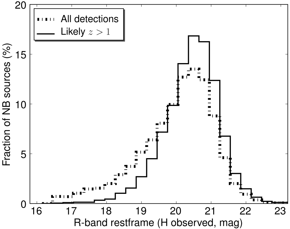
In S09, the entire range of sources detected in the narrow-band imaging was used to add line fluxes and then study the recovery rate. This can, nonetheless, be improved (as detailed in Section 4.2), to compute completeness corrections specifically for $z\sim 1.5$ sources. Here, that is done by i) excluding all stars (since they are not real $z\sim 1.5$ galaxies and they do not have their properties) and ii) excluding sources with colours which clearly place them clearly at $z<1$. By taking this approach, the observed H band magnitude distribution is quite different from that of all detections, as can be seen in Figure 22. Indeed, by using the entire population of detections, the number of bright sources with low equivalent widths is overestimated, and thus an overall lower completeness fraction is derived. Figure 23 compares the completeness fraction as a function of input line flux for simulations using all sources and for those using only $z>1$ galaxies (rejecting potential stars and using the $B$$R$$i$$K$ colour-colour selection).

Figure 23: A study of the completeness fraction (defined as the fraction of sources with a given flux recovered by the selection against the actual number of source with that flux) using two different input samples (all detections which are non-emitters and only those consistent with being $z>1$ sources).

References

- Aragón-Salamanca et al. (2003) Aragón-Salamanca A., Alonso-Herrero A., Gallego J., García-Dabó C. E., Pérez-González P. G., Zamorano J., Gil de Paz A., 2003 Vol. 297 of ASPCS, . p. 191
- Atek et al. (2010) Atek H., Malkan M., McCarthy P., Teplitz H. I., Scarlata C., Siana B., Henry A., et al. 2010, ApJ, 723, 104
- Bayliss et al. (2011) Bayliss K. D., McMahon R. G., Venemans B. P., Ryan-Weber E. V., Lewis J. R., 2011, arXiv:1102.0229
- Bertin & Arnouts (1996) Bertin E., Arnouts S., 1996, A&AS, 117, 393
- Best et al. (2010) Best P., Smail I., Sobral D., Geach J., Garn T., Ivison R., Kurk J., Dalton G., Cirasuolo M., Casali M., 2010, arXiv:1003.5183
- Brinchmann et al. (2004) Brinchmann J., Charlot S., White S. D. M., Tremonti C., Kauffmann G., Heckman T., Brinkmann J., 2004, MNRAS, 351, 1151
- Brocklehurst (1971) Brocklehurst M., 1971, MNRAS, 153, 471
- Bruzual (2007) Bruzual G., 2007, in A. Vallenari, R. Tantalo, L. Portinari, & A. Moretti ed., From Stars to Galaxies: Building the Pieces to Build Up the Universe Vol. 374 of Astronomical Society of the Pacific Conference Series, Stellar Populations: High Spectral Resolution Libraries. Improved TP-AGB Treatment. p. 303
- Bruzual & Charlot (2003) Bruzual G., Charlot S., 2003, MNRAS, 344, 1000
- Bunker et al. (1995) Bunker A. J., Warren S. J., Hewett P. C., Clements D. L., 1995, MNRAS, 273, 513
- Calzetti et al. (2000) Calzetti D., Armus L., Bohlin R. C., Kinney A. L., Koornneef J., Storchi-Bergmann T., 2000, ApJ, 533, 682
- Casali et al. (2007) Casali M., Adamson A., Alves de Oliveira C., Almaini O., Burch K., Chuter T., Elliot J., et al. 2007, A&A, 467, 777
- Chabrier (2003) Chabrier G., 2003, PASP, 115, 763
- Cutri et al. (2003) Cutri R. M., Skrutskie M. F., van Dyk S., Beichman C. A., Carpenter J. M., Chester T., Cambresy L., et al. 2003, 2MASS All Sky Catalog of point sources.
- Dale et al. (2010) Dale D. A., Barlow R. J., Cohen S. A., Cook D. O., Johnson L. C., Kattner S. M., Moore C. A., et al. 2010, ApJL, 712, L189
- Furusawa et al. (2008) Furusawa H., Kosugi G., Akiyama M., Takata T., Sekiguchi K., Tanaka I., Iwata I., et al. 2008, ApJS, 176, 1
- Gallego et al. (2002) Gallego J., García-Dabó C. E., Zamorano J., Aragón-Salamanca A., Rego M., 2002, ApJL, 570, L1
- Gallego et al. (1995) Gallego J., Zamorano J., Aragon-Salamanca A., Rego M., 1995, ApJL, 455, L1
- Garn & Best (2010) Garn T., Best P. N., 2010, MNRAS, 409, 421
- Garn et al. (2010) Garn T., Sobral D., Best P. N., Geach J. E., Smail I., Cirasuolo M., Dalton G. B., Dunlop J. S., McLure R. J., Farrah D., 2010, MNRAS, 402, 2017
- Geach et al. (2008) Geach J. E., Simpson C., Rawlings S., Read A. M., Watson M., 2008, VizieR Online Data Catalog, 838, 11369
- Geach et al. (2008) Geach J. E., Smail I., Best P. N., Kurk J., Casali M., Ivison R. J., Coppin K., 2008, MNRAS, 388, 1473
- Gilbank et al. (2010) Gilbank D. G., Baldry I. K., Balogh M. L., Glazebrook K., Bower R. G., 2010, MNRAS, 405, 2594
- Hayes et al. (2010) Hayes M., Schaerer D., Östlin G., 2010, A&A, 509, L5+
- Hogg et al. (1998) Hogg D. W., Cohen J. G., Blandford R., Pahre M. A., 1998, ApJ, 504, 622
- Hopkins (2004) Hopkins A. M., 2004, ApJ, 615, 209
- Hopkins & Beacom (2006) Hopkins A. M., Beacom J. F., 2006, ApJ, 651, 142
- Hopkins et al. (2001) Hopkins A. M., Connolly A. J., Haarsma D. B., Cram L. E., 2001, AJ, 122, 288
- Hopkins et al. (2000) Hopkins A. M., Connolly A. J., Szalay A. S., 2000, AJ, 120, 2843
- Hopkins et al. (2003) Hopkins A. M., Miller C. J., Nichol R. C., Connolly A. J., Bernardi M., Gómez P. L., Goto T., et al. 2003, ApJ, 599, 971
- Jansen et al. (2001) Jansen R. A., Franx M., Fabricant D., 2001, ApJ, 551, 825
- Kashikawa et al. (2004) Kashikawa N., Shimasaku K., Yasuda N., Ajiki M., Akiyama M., Ando H., Aoki K., et al. 2004, PASJ, 56, 1011
- Kewley et al. (2004) Kewley L. J., Geller M. J., Jansen R. A., 2004, AJ, 127, 2002
- Lawrence et al. (2007) Lawrence A., Warren S. J., Almaini O., Edge A. C., Hambly N. C., Jameson R. F., Lucas P., et al. 2007, MNRAS, 379, 1599
- Lilly et al. (1996) Lilly S. J., Le Fevre O., Hammer F., Crampton D., 1996, ApJL, 460, L1+
- Ly et al. (2011) Ly C., Lee J. C., Dale D. A., Momcheva I., Salim S., Staudaher S., Moore C. A., Finn R., 2011, ApJ, 726, 109
- Ly et al. (2007) Ly C., Malkan M. A., Kashikawa N., Shimasaku K., Doi M., Nagao T., Iye M., et al. 2007, ApJ, 657, 738
- Malkan et al. (1995) Malkan M., Teplitz H., McLean I., 1995, ApJL, 448, L5+
- McCarthy et al. (1999) McCarthy P. J., Yan L., Freudling W., Teplitz H. I., Malumuth E. M., Weymann R. J., Malkan M. A., et al. 1999, ApJ, 520, 548
- Mouhcine et al. (2005) Mouhcine M., Lewis I., Jones B., Lamareille F., Maddox S. J., Contini T., 2005, MNRAS, 362, 1143
- Ono et al. (2010) Ono Y., Ouchi M., Shimasaku K., Akiyama M., Dunlop J., Farrah D., et al.. 2010, MNRAS, 402, 1580
- Ouchi et al. (2008) Ouchi M., Shimasaku K., Akiyama M., Simpson C., Saito T., Ueda Y., Furusawa H., et al. 2008, ApJS, 176, 301
- Ouchi et al. (2009) Ouchi M., Shimasaku K., Akiyama M., Simpson C., Saito T., Ueda Y., Furusawa H., et al. 2009, VizieR Online Data Catalog, 217, 60301
- Ouchi et al. (2010) Ouchi M., Shimasaku K., Furusawa H., Saito T., Yoshida M., Akiyama M., Ono Y., et al. 2010, ApJ, 723, 869
- Ouchi et al. (2004) Ouchi M., Shimasaku K., Okamura S., Furusawa H., Kashikawa N., Ota K., Doi M., et al. 2004, ApJ, 611, 660
- Pettini & Pagel (2004) Pettini M., Pagel B. E. J., 2004, MNRAS, 348, L59
- Rola et al. (1997) Rola C. S., Terlevich E., Terlevich R. J., 1997, MNRAS, 289, 419
- Shioya et al. (2008) Shioya Y., Taniguchi Y., Sasaki S. S., Nagao T., Murayama T., Takahashi M. I., Ajiki M., et al. 2008, ApJS, 175, 128
- Simpson et al. (2006) Simpson C., Martínez-Sansigre A., Rawlings S., Ivison R., Akiyama M., Sekiguchi K., Takata T., Ueda Y., Watson M., 2006, MNRAS, 372, 741
- Smail et al. (2008) Smail I., Sharp R., Swinbank A. M., Akiyama M., Ueda Y., Foucaud S., Almaini O., Croom S., 2008, MNRAS, 389, 407
- Sobral et al. (2010) Sobral D., Best P. N., Geach J. E., Smail I., Cirasuolo M., Garn T., Dalton G. B., Kurk J., 2010, MNRAS, 404, 1551
- Sobral et al. (2009a) Sobral D., Best P. N., Geach J. E., Smail I., Kurk J., Cirasuolo M., Casali M., et al. 2009a, MNRAS, 398, 75
- Sobral et al. (2009b) Sobral D., Best P. N., Geach J. E., Smail I., Kurk J., Cirasuolo M., Casali M., et al. 2009b, MNRAS, 398, L68
- Sobral et al. (2011) Sobral D., Best P. N., Smail I., Geach J. E., Cirasuolo M., Garn T., Dalton G. B., 2011, MNRAS, 411, 675
- Straughn et al. (2011) Straughn A. N., Kuntschner H., Kümmel M., Walsh J. R., Cohen S. H., Gardner J. P., Windhorst R. A., et al. 2011, AJ, 141, 14
- Tadaki et al. (2011) Tadaki K.-I., Kodama T., Koyama Y., Hayashi M., Tanaka I., Tokoku C., 2011, PASJ, 63, 437
- Takahashi et al. (2007) Takahashi M. I., Shioya Y., Taniguchi Y., Murayama T., Ajiki M., Sasaki S. S., Koizumi O., et al. 2007, ApJS, 172, 456
- Teplitz et al. (2003) Teplitz H. I., Collins N. R., Gardner J. P., Hill R. S., Rhodes J., 2003, ApJ, 589, 704
- van Breukelen et al. (2007) van Breukelen C., Cotter G., Rawlings S., Readhead T., Bonfield D., Clewley L., Ivison R., Jarvis M., Simpson C., Watson M., 2007, MNRAS, 382, 971
- van der Werf et al. (2000) van der Werf P. P., Moorwood A. F. M., Bremer M. N., 2000, A&A, 362, 509
- van Dokkum et al. (2011) van Dokkum P. G., Brammer G., Fumagalli M., Nelson E., Franx M., Rix H.-W., Kriek M., Patel S., et al. 2011, arXiv:1108.6060
- Yagi et al. (2002) Yagi M., Kashikawa N., Sekiguchi M., Doi M., Yasuda N., Shimasaku K., Okamura S., 2002, AJ, 123, 66
- Yamada et al. (2005) Yamada T., Kodama T., Akiyama M., Furusawa H., Iwata I., Kajisawa M., Iye M., Ouchi M., et al. 2005, ApJ, 634, 861
- Yan et al. (1999) Yan L., McCarthy P. J., Freudling W., Teplitz H. I., Malumuth E. M., Weymann R. J., Malkan M. A., 1999, ApJL, 519, L47
- Zhu et al. (2009) Zhu G., Moustakas J., Blanton M. R., 2009, ApJ, 701, 86